This document provides an overview of the theory and practice of foundation design. It discusses soil as an engineering material, including soil classification, properties, testing, and deposits in India. It also covers site investigation techniques, soil data analysis, types of foundations, stress distribution in soils, bearing capacity of shallow foundations, settlement analysis, design of footings and raft foundations, pile foundations, well foundations, expansive soils, and ground improvement techniques. The book is intended as a reference for civil engineers on the topic of geotechnical engineering and foundation design.

1. THEORY
AND PRACTICE OF
N.N. SOM • S.C. DAS

2. Copyrighted material

3. Theory and Practice of
Foundation Design
T h.1e
On e

4. Copyrighted material

5. Theory and Practice of
Foundation Design
N.N. SOM
Prof.ssor of Civil Engin<ering
Jadavpur Univ~rsity, Kolkala
S.C. DAS
Professor of Civil Eng inuring
JiUUJvpur UniverJ;ry, Kolkalo
Prentice, Hall of India ~ [lli[U)~
New Delhi - 110 001
2006
Copyrighted material

6. Rs. 275.00
THEORY AND PRACTICE OF FOUNDATION DESIGN
by N.N. Som and S.C. Das
0 2003 by Prentic&>Hall o1 India Private limited., New Delhi. All tigh!S resetved. No part ol tNs bOOk
may be reproduced il 8frJ fonn, by mimeograph or any other meens, vNiout permission h writing
from the J)l.C)Iistwtr.
ISB,..._I1-203·2191)..1
The export l"ighls ot this book are vested solely with the publiShet.
Thh'd Printing
June, 2006
Published by Asoke K. Gh0$h. Prentice-Hall ot India PMte Umited. M-97, COnnaught Circus,
New Oelhl-1 10001 and Printed by Jay Print Pack Private Limited, New Oelhi-110015.
Copyrighted material

7. To
Professor NOEL E. SIMONS
and
Indian Geotechnical Society

8. Copyrighted material

9. Contents
Prtau
I
SOIL AS AN ENGINEERING MATERIAL
1
I I
Introduction
I 2
N amrc of Soil
1.3
Th~ phase
1.3. 1
1.3.2
2
System J
Defiojcjons 4
Weight/Volume Relationships
1.4
S
1.6
Soil C lass jfication
4
Index Propenies of Soil 4
1.4.1 Plasticity Chan 6
1
7
Relative Density of Granular Soil 8
I. 7 Some Special Soil Types 9
1.8 Groundwater /0
1.8.1 Types of Water-bearing Formations 10
I 82
Ojy jsjon of Subsurface Water I I
1.9 Engineering Properties of Soil /2
1.9.1 Permeability /2
1.9.2 The Principle of Effective Stress JJ
1.9.3 Pore-pressure in Soil due to Applied Lood
1.9.4 Shear Strength of Soils /7
1.9.5 COM(')Iidation 21
1.9.6 Properties of Soil 26
1.10 Soil Deposits of India 29
Rel~renceJ 30
2
I-3I
SITE INVESTIGATION
/6
32-53
12
2.1
Jotmductjon
2.2
2.3
Information Extracted from Site Investigation 32
Stages of Site Investigation 3.1
2.3.1 Reconnaissance Study 33
Boring (Detailed Soil Investigation) 34
2.4
J4
2 4 1
Trial Pirs
2.4.2
Wash Boring
J4
Ytl
Copyrighted material

10. YIU • Ctmteuu
2.6
2.4.3 Auger Boring 35
2.4.4 Rotary Drilling 36
2.4.5 Percussion Drilling 36
2 4 6
Srahiljz;)tjon of Boreholes l6
Sampling 37
2.5. 1 Sampling from Trial Pils 37
2.5.2 Sampling· from Boreholes 37
2.5.3 Preservation of Samples 39
Testing of Soil 40
27
Field Iesrs
2.5
41
2.7.1
2. 7.2
2.7.3
2 7 4
Vane Shear Test
2.7.5
2.7.6
Direct Shear Test (In-situ) 47
Plate Bearing Test 48
2 7 7
2.8
Standard Penetration Test <SPD 41
Dynamic Cone Penetration Test (DCP1J 43
Static Cone Penetration Test (SC!'D 44
J?u:ssurc:merer Tesr
46
49
Lahoratory -Tests 51
51
2.10 Planning of Exploration Programme 51
2.10.1 Layout and Number of Boreholes 51
2.10.2 Depth of Boreholes 52
2 9
Ground Water Table
Rtkrtncu 53
3
SOT!. DATA AND DFSJGN PARAMETERS
3. I
Introducrion
54
Soil Investigation 55
3.2.1 Responsibility of Designer 55
3.2.2 Information Required from Soil lnveotigation 55
3.2.3 Soil Test Report 55
Reference 64
3.2
4
FOUNDATIONS: TYPFS AND DESIGN CRITERIA
4.1
4.2
Jnu!lduction 65
Iypes of Foundation 65
4.2. I
4. 3
65- 75
Shallow foundadons 66
Deep Foundations 68
4.2.2
4.2.3 Choice of Foundation Type 70
Design Criteria 70
4.3.1 Bearing Capacity 70
4.3.2
The SenJemeoJ Criteria
71
References 75
Copyrighted material

11. Contellls + ix
5
STR FSS QISTR IB I rtiON IN
sou s
76:116
76
5 I
Introduction
52
5.4
76
Stresses due to Foundation Loading 78
5.3. 1 Boussinesg Analysis: Point Load 78
Venical Stresses below Unifonn Rectangular Load 8/
SS
Vcnical Srrcsses below IJnj form Circular l nad
5.6
Other Common Loading Types 85
5 6 I I fnjform I joe I oad 85
5.6.2 Unifonn Strip Load 85
5.6.3 Triangular Load 86
5.6.4 Embankment Type Loading 87
Stress at any Point below Rectangular Load 89
5.3
5. 7
S8
S9
In-situ Srress
8!
Newmark's O,an 89
Pressum Bulb 9/
5.10 Rigidity of Footings: Contact Pressure 92
5.1 I Non-homoge.neous Soils 94
5.11.1 Two-layer System 94
5.1 1.2 Three-layer Systems 97
5.1 1.3 Multilayer Systems 99
5.11.4 Non-homogeneous Medium /00
5 12 Nonljnear $ojl
/Ot
5. I 3 Approximate Method of Detennining Venical Stress
Re(erenc~s
6
/06
11)
BEARING CAPACITY OF SHA!.I.OW FOUNDATIONS
6 I
62
l ntrodnrljno 117
Fajlure M ecbanjsril
117-137
118
6.2.1
6.2.2
6.2.3
6.2.4
Prandtl's Analysis 120
Terzaghi's Analysis 122
Skempton Method 125
Meyerhors Method 125
62 S
Ham;en·s M ethod
6.2.6
Vesjc's Method
/26
126
6 3
1 «a! Shear Eajlure
6.4
6.5
Square and Circular Footings
6.6
Limitations of Theoretical Analysis
6.7
Factors Affecting Bearing Capaciry /29
6.7. I Effect of Ground Water Table on Bearing Capacity 130
Gross and Ne.t Soil Pressure: Safe Bea.ring Capacity 131
Bearing Capacity from Field TestS I 3 I
6.8
6.9
126
127
Bearing Capacity of Non·homogeneous Soil
127
/29
R•fere11ces /36
Copyrighted material

12. x + Comenu
7
SETI'LEMENT ANALYSIS
7 I
7.2
lntrOOnctinn 1 JR
7 I I
Definjrjons
138- 163
118
7. 1.2 Methods of Settlement Analysis I 19
Stress-path 141
7.2. 1 Stresses During loading and Consolidation in the Field
7 .2.2 Influence of Stress-path on the Drained Deformarion
of Clav 148
7.2.3 Settlement Analysis by Stress-poth Method 149
7,3
Rote of SettlemenJ
7 ,4
Foundatjon on Sand
7 .4.1
7 .4.2
146
151
152
Elastic Theory I 52
Semi-empirical Method (Buisman. 1948)
7,4.3
Plate Load Test
74 4
Stj)tjc Cone Tt-SJ
I 52
/ 51
151
Re(trenets 161
8
FOOTINGS AND RAFI' DESIGN
164-!98
164
8 I
lntmductjon
8.2
Design
8.2. 1
8.2.2
8.2.3
of Footings 165
Depth of Footing /65
Allowable Bearing Capacity 166
Effecl of Ground Wa1er Table 168
82 4
Senlement
8.2.5
8.2.6
8.2. 7
8.2.8
De.<ign
8.3.1
8.3.2
Dimens ioning Footing Foundations 170
l nterfcrenre Effect /72
Design for Equal Settlement 172
Structural Design of Footings 174
of Raft Foundation 175
Types of Rllft Foundation 175
Bearing Capacity 177
8.3
169
177
8 .3.3
Scttlcmenl
8.3.4
Aoating Foundation
8.3.5
Basement Raft
178
/81
8.3.6 Structural Design of Raft Foundation
Referenc-. I 98
9
182
PIJ.E FOUNDATIONS
9 I
9.2
9.3
lntroductjon 199
C!qs..,jfie.ation 200
9.2. L Classi fication Based on Composition 200
9.2.2 C!assjficatjoo Based on Merbod of lnsta!larjoo
Pile Behaviour Under Axial J.ood 201
199- 265
201
Copyrighted material

13. Coments • xi
9.4
9.5
Pile Capacity to Resist Axial Forces 203
9.4.1 Structural Capacity of Piles 203
9.4.2 Pile Capacity from Static Analysis 203
EricljonaJ Resjs(inee 206
9,5. I
9.5.2
Fric1jonal Rcsjstance jn Cohesjve Sojl 207
Frictional Resistance in Cohesionless Soil 210
9.7
9.8
End Bearing 2I 3
9.6.1 End Bearing in Cohesive Soil 2/3
9.6.2 End Bearing in Cohcsionless Soil 213
Critical Depth 215
Pile Capacicy from l n-siw Soil Tests 217
2 .9
Under-reamed Pj!es
9.6
21 7
9.10 Allowable Load on Piles from Static Analysis 218
9.11 Dynamics of Pile Driving (Dynamic Analysis) 2/9
9. II.! ENR Formula 220
9.11.2 Hiley Formula 22/
9.11.3 Simplex Formula 22/
9.1 1.4 Janbu's Formula (Janbu, 1953) 222
9.1 1.5 Wave Equation 222
9.1 1.6 Umitations of Dynamic Analysis 223
9.12 Pile Groups 223
9.12.1 Capacity of Pile Group 224
9. 12.2 Pile Spacing 225
9.12.3 Pile Group Subjected to Vertical Load and Moment 227
9.13 Senlement of Pile Groups 228
9.13.1 Pile Groups in Cohesive Soil 228
9.13.2 Pile Groups in Cohesionless Soil 230
9.14 Uplift Resistance of Piles 231
9. 15 Piles under H orjzoocal Forces 232
2 .15.1 Faj!ure Mechanisms 232
9.15.2 Stiffness Factors and Subgrade Modulus 233
9. 15.3 Uhjmate Laleral Resistance
234
9.15.4 Deflection, Moment, and Shear under Working Load 237
9. 15.5 I.S. Code MeJhod 240
9.16 Negative Skin Friction 242
9.17 Testing of Piles 245
9.17.1 Purpose of Pile Testing 246
9.17.2 Causes of Defect in PHes 246
9.17.3 Integrity Testing 246
2 . 18 Load Test on Piles
247
9.18.1 Test Procedure 248
9.18.2 Maintained Load Test 248
9. 18.3 Constant Rate of Penetration (CRP) Test 249
9. 18.4 Pile Driving Analyzer 251
R•for.nus 262
Copyrighted material

14. IXii • Cnntem.r
10
266-293
WELL FOUNDATIONS
10 I
10 2
lntrodncrjon 266
C lassificarjon 266
I 0.3 Physical CharocteriSLics-shape and Size
10.4 Componen<s of Well Foundation 268
10.4.1 Steining 269
10 4 2 Well Curb
10.5
I 0.6
I 0. 7
10.8
10.9
267
269
10.4.3 Culling Edge 269
10.4.4 Bouom Plug 269
10.4.5 Dredge Hole 269
10.4.6 ln<ermediatefl'op Plug 270
10.4.7 Well Cap 270
Sinking of Wells 270
Physical Characteristics-Depth 270
10.6.1 Scour Depth 270
Allowable Bearing Pressure 27I
Forces Acting on Well Foundatlon 272
Lateral Stability 273
10.9.1 Analysis Based on Bu.lkhead Concept 273
I0 9.2 IRC Method 275
10.9.3 Mode of FaUure 281
10.9.4 Recommeodarjons of IRC. 78-. 1283
281
10.10 Well Sinking 283
References 293
II
294=303
FOUNDATIONS ON EXPANSIVE SOII.S
I I I
lntroductjon
294
11.2 Nature of Ex)?!lnsive Soil 294
1L
.2.1 fret·swell Test
294
11.2.2 Differential Free Swell 295
I I 2 3 t Jnrestmjned Swell Tcsr 295
11.2.4 Swelling Pressure 296
11.2.5 Cla.•sification of Swelling Potential 297
11.3 Effect of Swelling on Building Foundations 297
I 1.4 Foundation Design in Expansive Soil 298
11.4.1 Isolating the Foundation from the Swelling Zone:
Under-reamed piles 298
11.4.2 Controlling Swelling 300
I J .4.3
Me.a~ures
to Wj!hstand Seulernent
102
Re[uences 302
12
GROUND IMPROVEMENT TECHNIQUES
12 I
lntaylucrjon
304=345
10:1
I 2.2 Principles of Ground Improvement 304
12.3 Ground T renJment i n Cohesive Snj!
106
12.3.1 Preloading with Venical Drains 306
I2 3 2
Sronr O J!umns
V4
Copyrighted material

15. Conttllf.f + xiii
12.4 Ground Improvement in Granular Soil 326
12.4.1 Heavy Tampir.g or Drop Hammer 326
12.4 .2 ·Dynamic Consolidation 328
12.4.3 Vibroeompaction 330
12.4.4 Compaction Piles 332
12.4.5 ConlrOI of Field Work 332
Rtkr~nus
13
344
EART HQUAKE RESPO NSE OF SOILS AND FOUNDATIONS
13.1 lnlrOduction 346
13.2 Earthquake Characteristics 346
13.2.1 Magnitude 346
13.2.2 Energy Release 347
13.2.3 Intensity 347
13.2.4 Ground Acceleration 348
13.2.5 Response Spectrum 348
13.3 Effects of Earthquake 350
13.4 Ground Settlement 350
13.5 Liquefaction 352
13.5.1 Liquefaction Potential 354
13.6 Effect of Earthquake Loading on Behaviour of Fine-grained Soils
13.7 Building Damage due to Liquefaction 360
13.8 Measures to Prevent Liquefaction 362
13.9 Effect on Superstructure 362
13.10 Dynamic Properties of Soil 363
346-370
358
ReJere11ces 369
14
CONSTRUCTION PROBLEMS
14.1 lntroduction 371
14.2 Common Construction Problems 371
14.3 Stability of Excavation 372
14.3.1 Design of Bmced Cuts 373
14.4 Dewatering 378
14.4.1 Rate of Seepage 378
14.~.2 Methods of Dewatering 380
14.4.3 Field Con1r0l 384
14.5 Land filling 385
14.5. 1 Cohesive Fill 385
14.5.2 Granular fill 387
14.6 Effect on Adjoining Structures 389
14.6. 1 Effect of Vibration 391
R~f
tmmces 392
371-392
Appendix
393-394
lntfu
.195 .!99
Copyrighted material

16. Copyrighted material

17. Preface
Over long years of association with the profession of teaching and research in civil and
geotechnknl engineering. our experiences sugges1 that foundations arc ofte- designed without
n
lllking all the ess<:nlial parameters into consideration particularly those with regard to geology
of the site. soi.l dara! ground conditions. type of structure. and )and use pattern in the vicinity of
the construction area. Though the theoretical aspects of foundation design are well understood.
the fie ld situations are usually not given the due imponance. As a c·o nsequence, the
implementation of the proposed design runs into problems necessilllting changes in constrUction
methodology or in some cases. even the design.
The book covers the essentiaJ features of foundation design through fourteen chapters.
The foundation design requires underslJinding of the soil type, its strength and deformation
characteristics. ground wate- tab1e, and other details of the site and the structures. We have
r
striven to incorporate all these criteria so as to acquaint the reader with all necessary aspects or
foundation design. This treatment begins with Chapter I that details the engineering properties
of soil as required for the design of sound foundations. Chapter 2 discusses site investigation as
lhe next step towards foundation design. This chapter elaborates on the various methods of soil
exploration and testing. The design parameters and the importance of proper interpretation of
the data collected from soil i11vestigation arc described in Chapter 3 while Chapter 4 introduces
different types of foundations and lheir charac.tetistic- .
s
Chapters S through 7 offer de<ailed study of the mechanical prope11ies of soil including
the stress distribution, the bearing capacity of foundations, and settlement. The effect of non~
homogeneity and nonlinearity of the stress-strain relationships on the stress distribution in soils
is elucidated and the concept of streSS-path method of settlement analysis is introduced in these
chapters. The imponant considerations for obtaining the design parameters from a Jarge amounl
of soil test data are highlighted. The design procedures for shallow and deep foundations. a..;;
also for well foundations are presented in Chapters 8 through 10. The special requirements of
expansive soils are covered and the earthquake response or soils and foundations are empha..;;ized
in Chapters II and 13 respectively. The ground improvement techniques commonly used in
practice and the constJUCtion problems generally encountered at site are adequately dealt with in
Chapter 12. The reader should also find in the book a comprehensive treatment or the design
procedures
vis~ a ~vis
the construction problems and practices (as discussed in the final chapter).
The chapters on analylical aspects are followed by worlced-out examples taken from real-life
problems which make the reading bolh topical and interesting. Besides, numerous references
have been made to actual cases of foundations for better clarity and understanding of the topics
covered.
XV
Copyrighted material

18. xvi • Preface
We have drawn upon our experiences in teaching and consultancy in geotechnical
engineering to compile this volume. Almost forty years of tcachjng and research at Jadavpur
University have given us the opportunity to face many field situations which hod to be treated
in unconventional ways. The inter.&
ction with our students has been very helpful during all these
years. This book is designed to serve undergraduate and postgraduate students of civil
engjneering with interest in foundations-their design, development, and maintenance. lt will
be equally useful for practising civil and structural engineers who have to design fou ndations of
structures in difficult subsoil conditions.
We acknowledge the immense help derived out of our association with colleagues
in che civil engineering department at Jadavpur University, Kolkata. We are thankful to
Prof. R.O. Purkayastha, Prof. P. Bhattacharya, Prof. S.C. Chakraborty, Prof. S.P. Mukheljee.
Or. S. Ghosh, and Or. R.B. Sahu who participated in many fruitful discussions on the
subject and gave their invaluable suggestions. We are also grateful to our staff at the soil
mechanics division. particularly Mr. Robin Pal, Mr. Apurba Banerjee, Mr. Sisir Monda ),
Mr. Ranm Jana, and Mr. Bhupesh Ghosh for their skilled help in many ways. The painstaking
task of compiling the manu.~eript was undertaken by Mr. Bivas Roy, Mr. Subhasish Ghooh, and
Mr. Hrishikesh Nayak with great interest and patience. We express our sincere thanks to
them all.
Last but not the least, we express our sincere gratitude to our spouses Smt. Rita Som
and Smt. Sikha Das for bearing with the demand of time that was needed to complete the
task often under trying circumstances.
N.N. SOM
S.C. DAS
Copyrighted material

19. Soil as an Engineering
Material
1.1 INTRODUCTION
From an engineering viewpoint. soils and sof1 rocks comprise all the loose ond fra-gmented
materials that are fou nd in the em1h's crust They arc distinguished from solid rock. i.e., the
hnrd ond compnct mass i n the earth's body, which cannot normally be excavated by manual
means. Soils 3re fonned by disintegr:uion or decomposition of a parent rock by weathering
or they moy be depOsited by cr:mspOnation from some other soun.·e.
Soils which are formed by the disintegration of 3 parent rock and remain 01 their place
of formation are known as re.sidual soils. The disintegration of the. parent rock is caused by
physical agents such as tempcroture changes. freezing. thawing etc. or by chemic.al agents like
ox.id:.uion, hydration etc. When the soil is transpOned from its original bed rock by forces of
gravity. wind, water or ice and re-deposited at another location it is known as tra11sporttd
soU. Tmnsported soils arc gcnerully sorted out according to their gmin s ize as the velocity of
the transporting medium gets reduced away from the source. A fter deposition at a new place,
these soils may be subjected to further weathering with the passage of time.
Tnmsported soils tare c lassified into differe nt types according ro their mode of
1
ransponmion. r.>eposits of soil thar nre formed by willd 11re called Aeolian deposi1s. Sand
dunes and loess are examples or these de.positS. Loose sand is geJle.rally swept by wind and
transported close to the surface. If the motion is stopped. it is depOs ited in the form of sand
dunes. The common lrllllSported soils are, however, those which have been carried by water
or ancient glaciers. Mariue soils which have been can·ied by sea w:atcr and Alluvial soils
which have been carried by rivers 3nd streams constilute probably the largest group of
transpor1ed soils on earth. These deposits may also be called sedimemary deposits ns they
hnve be.en formed by deposition from e ither standing or moving water. The deposilion is
primarily caused by the graduaJ decrease in 'elocity or river carrying the sedi ment~. A larger
part of the great Indian plains is made up of alluvial deposits. Gltrcinl deposit~ are remnants
of the icc age thai were carried along by the moving ice. They are generally found as big
boulders at places away from their parent rock and nrc heterogeneous in nature with linle or
no stratification. Other sedi mentary deposits :;ti'C the Lacustrine .soils which are depos ited on u
lake bed and the Esluaritre soils which arc deposited at the mouth of ::tn estuary.
1
Copyrighted material

20. 2 • Theory and Practice of FoutJdatiou Desig11
1.2 NATURE OF SOIL
Properties of soil are complex and variable, being primarily infl uenced by the geological
environment under which they have been deposited. An understanding of soil composition is
important in appreciating the mechanic.al behaviour of the soil. Natural soil consists
essentially of discrete solid particles which are he.ld together by water and/or ga.< filling the
pore space. These particles are. however. not bonded as strongly as the crystals of a metal are
and can. therefore. move freely with respect to one another. The si?.e :md shape of grains and
the minemlogical composition of soil panicles varies widely in nature. However. in c.oarsegrained soils the most important propenies do not depend on the constituent minerals
although locally, the minerals may control the frictional c- aracteristics of the individual
h
grains. In these soils, the panicles are so large that the forces between the grains other than
those due to externally applied forces and gravity are smaJI. The non.day minerals suc.h as
mica. feldspar, and quanz which constitute sand and silt do not render any plasticity and
cohesion to the soil. Thus. the influence of the constituent minerals becomes appreciable with
the decrease in size.
Clay minerals are hydrated aluminium silicates in crystalline form. These are generally
of three different types (Scott 1965):
A 14 Si0 4 0 1o(OH)a
Kaolinite
Montmorillonite : (AI~.67 MgNao.33)Si,0 10(0H)1.H20
Ulile
K,(AI4 Fe4 Mgu)(Si8_7 I y)0 20(0 H),
.A
Kaolinite has a very stable struciUrc. h generally resists the ingress of water and
consequently, undergoes little volume chan,ge whe,n in contact with water. On the other hand,
Montmorillonite auracts water and undergoes large swelling and expansion when saturated
with water. Most of the black cotton soils of India contain clay minerals of this variety. Illite
is less expandable than montmorillonite.
A s ingJe panicle of clay consists of many s heets of clay mine,rals piled one on another,
as shown in Fig. 1. 1. As each sheet has a definite thickness but is large at right angles to itS
thickness. clay particles are believed to be plate shape:d. The Oat surfaces carry residua)
negative charges, but the edges may carry either positive or negative charges depending upon
the environment
4
":w=o::::oooc:o=; Potasslum
'
L,r----~ Strong
r - - - o - l>OO<I
Weak
bOOd
(a) Kaolinite
"-'r-----{/ Slrong
r---o-bond
(
molecules
":w:=-:=c:o::::Jc:~ Fa;rty strong
'<
bond
) =weak
<:Jooc::c:c:~ Potassium
I
'(b) Montmorillonite
Fig. 1.1
~
molecules
(c) tulle
Structure of day particles.
Copyrighted material

21. Soil as 011 E.11ginetri11g Maten'al • 3
Particle orientation has an imponant bearing on the engineering properties of a soil.
Spacing 1nd orientation of panicles influence the development of interparticle bonds. For
cohes.ionless soils. individual grains may be approximated as spheres with loose. dense, or
honeycombed structure, as shown in Fig. 1.2. A dense structure is more stable than the loose
or honeycombed structure. Figure l.3 shows some simplified structures found in clay. The
development of structure is influenced by the origin and nature of deposition of the soil.
Thus. the flocculated structure is typical of clay deposits in salt water. This structure may
change due to leac.hing or by external influences. auch as loading, drying. freezing. electroosmositic processes. and so on.
(a)
(c)
(b)
Fig. 1.2 S bwture of c:oheslonle$$ soits.
(a)
(b)
Fig. 1.3 Structure of
eohesl~
SOilS.
1.3 THREE-PHASE SYSTEM
Figure L4 shows a typical soil skeleton consisting of three distinct phases-solid(mineral
grains). liquid(usually water). and gas(usually air). These phases have been separated to
facilitate the quantitative study of the proportional distribution of different constituents.
Fig, 1.4
Thre&1)t'lase system,.
Copyrighted material

22. 4 + Tlteory and PmCiice of Foundation De.sigu
1.3.1
Definitions
r.. =
Water
(a) Unit weigh~
W..,IV.,
Solid particles
r,= WsfV1
Specific gravity : Gs =
= W,IV"y_.
rirw
(b) Water conte.nt.
IV = (W.IWJ x 100%
(c) Void ratio,
e = Vl'IV_, = (V., + V8 )/V"
n = V,JV = V/(V, + V,)
S = V.JV, = V.I(V. + V )
1
(d) Porosity,
(c) Degree of sawnuion.
1.3.2
(a)
Weight/Volume Relationships
11
( b) Se
= el( I
+ e) or
=n/( I
- n)
= wG,
(c) Bulk de nsity.
r=
(d) Dry density. 1fl =
(e)
e
r= (I
W
+
v = Se1 + G, )( r.
e
~
=
G,
1 + t0
r.
X
+ w) Yd
( f) Submerged densi<y,
r' = r - r.
c
.
(G - I) - (I - S)e
I
I
For saturated soil, S = 1.0.
...
X
r•
G - I
.
r'= t.f+ e x y_.
The range over which the typical values of the above parameters vary are as follows:
(i) G,= 2.60-2.75
r
(ii)
= 1.60-2.25 glee
= 1.30- 2.00 glee
(ii i)
(iv) " = 0.25-0.45 (for sand)
0 (for dry soil}-100% (for fully saturated)
(v) S
r,
=
1.4 INDEX PROPERTIES OF SOIL
As already menrioned. the clay minerals in fine-grained soils have sufficient surface forces to
attract water molecules to the clay particles. The interaction between the clay minerals, water.
and various chemicaJs dissolved in the water is primarily res ponsible for developing the
consistency of these panicles.
Pure water mainly consisL.:; of molec- les of H1:0 but a few of them get dissocialed iniO
u
hydrogen ions, H+ and Hydroxyl ions. 0 11. If impurities such as acids and bases are present.
Copyrighted material

23. SoU as au Eugiuuring Maltrial + 5
they also dissociate into cations and anions. Sail. for example. breaks up into Na• and CJ- .
Since plane surfaces of the clay mineials carry negative charges, cotions including H+ from
water are attracted towards the surface of these particles. The water molecules closest to the
clay particles. called the adsorbed water. are tightly held to the clay and exhibit propenies
which are somewhat different from those of ordinary wa:er. This adsorbed water is believed
to give cohesive and plastic propertie~ to clayey soils. It is obvious, therefore. that the
amount of water present in a clay will determine its plasticity characteristics and. in tum. ilS
engineering properties. The Atterberg limits are designed to serve as an index of the
plasticity for clayey soils. refer Fig. 1.5.
Plastic
5em1Uquld
state
stale
! - - - - + - - -;.....----;.....--+Increase of moisture
Solid state,
SemiSOid
state
content
Legend
Sl-Shri'lkage limit
PL~astic limit
U -4.iquid limit
Moisture content
Fig . 1.5 limits of consistency.
Slarting with a low water content a clayey soil first appears to be a solid and moves to
the plastic state with increasing water contenl. The word plastic here refers to the ability of
a soil to be moulded into different shapes without breaking up. At even a higher water
content. the soil begins to flow as a viscous fluid. The Atterberg limits. that is, the liquid
limit (LL), the plastic limit (PL), and the shrinkage limit (SL) indicate the limits of water
content at which the consistency of clayey soil changes from one state to another.
The Atterberg limits along with the natural water content give useful indication of the
nature of the clayey soil. A natural water content close to the liquid limit indicates a soft
compressible soil while a natural water content close to the plastic limit is characteristic of a
stiff and Jess compressible c lay.
Plaoticlty Index, PI
The range of water content over whic- a soil remains plastic is called the plastic limit.
h
i.e.
PI = U - PL(%)
( 1.1 )
Liquidity Index, LI
It is the ratio of natural water content, w of a soil in excess of its plastic limit to its plasticity
index and is indicative of the state of the water c.ontent in relation 10 the liquid limit and the
plastic limit of the soil.
U=
IV -
PL
LL- PL
X
100%
( 1.2)
Copyrighted material

24. 6 •
11r~ory
1.4.1
and Practice of Fourul.arion De.sigll
Pluticity Chart
It has been observed that propenies of clay and s ih can be correlated at least qualitatively with
the Auerberg limits by means of the Plruricil)l Chart, as shown in Fig.l.6. The liquid limit and
h
the plastic limit or a soil are ploned on the plasticity c- art and the soil is classified according 10
the region in which it falls, the A-line being an arbitrary boondary between inorganic clays and
inorganic silt/organic c lays. Table 1.1 gives the liquid limit of some cohesive soils.
70
//
60
~
U-lino
50
PI • 0.9 (LL - 8}
Ci:
'>
~ 40
~
i
l
30
/
/
20
10
0
0
. /!
10
/
'
v
20
CL
or
OL
/,
Cl-ML
/
/
/
/
or
OH
/'
/
/
A-tine
PI • 0.73 (LL - 20)
v,;
L
MH
or
or
OH
OL
30
/
CH
/
40
50
60
Liquid limit, LL (%)
70
60
90
100
Fig. 1.8 Plasticity chart
Table 1.1
Soil
Consistency limits of some soils
Liquid Limit (~)
Plastk Limit (e.fl)
Alluvial Deposits
Boston Blue Clay
Chicogo Clay
Normal CaJcuua Soil
41
20
,S8
21
55
28
MariMIE.'Itwtrint
London Clay
75
Norwqian Quick Clay
Bombay M:uine Cay
Cochln Marine Clay
Shellbaven Clay
40
90
Illite
Kaolinite
MontrooriJJonite
29
17
90
40
45
97
)2
Clay Minerals
100
45
so
25
500
50
Copyrighted material

27. 8 •
Tlu~ory
and Practice of Fouudatio11 Desig11
Sand
Gravel
100
.........__
'
['
.: eo
1
];
60
~
~
&
~
~
6
10
0.6
2
-.... k I
j'"'j
0.2
0.06
0.1
1
0.02
.........__
t'
Oispeo>ed
kaolinite
Ctaye~
I'-
0
sandy silt
I
Flocculated
Gra¥elty
sand
20
..... '""--J~montmo1111onlte)
00•um ~ton""'
'
Silty
ne s*nd
Ctay
nne
r---
['
"()
!'I
c
..
Silt
fine coarse meclk.m
ooarse
"'
.......
0.006 0.002
0.01
....
'
0.0006
0.001
0.0001
Particle diameter {mm)
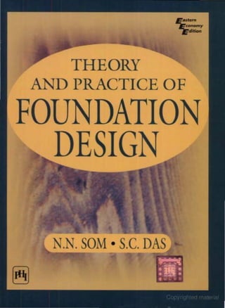
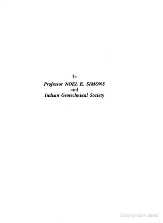
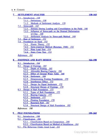
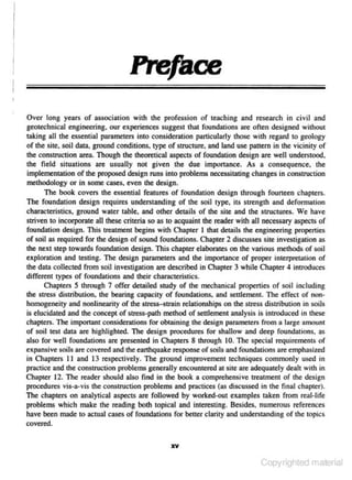
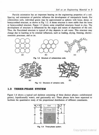
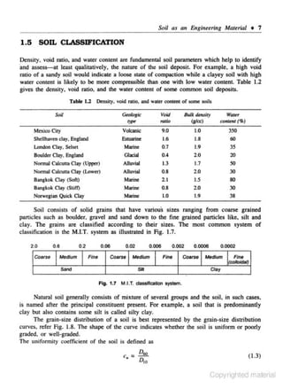
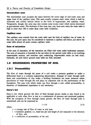
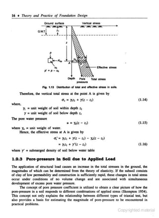
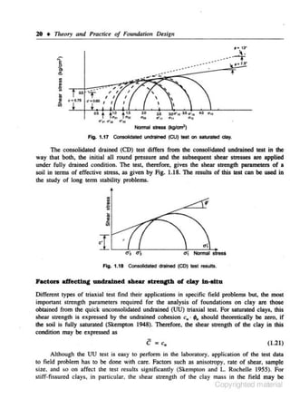
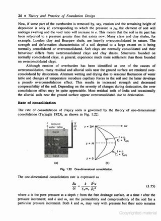
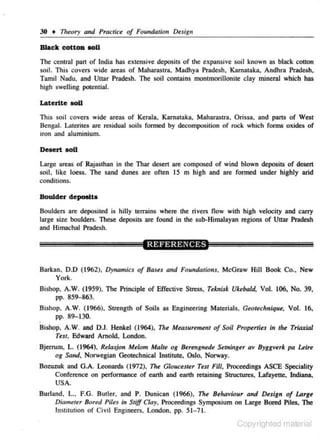
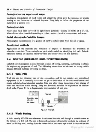
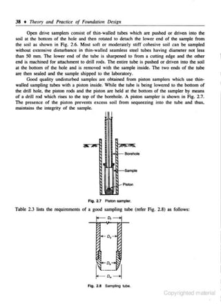
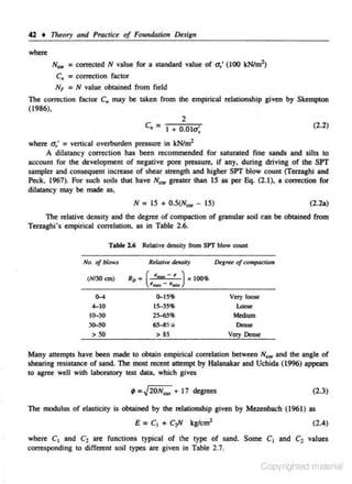
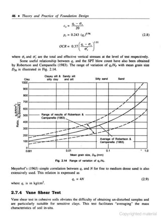
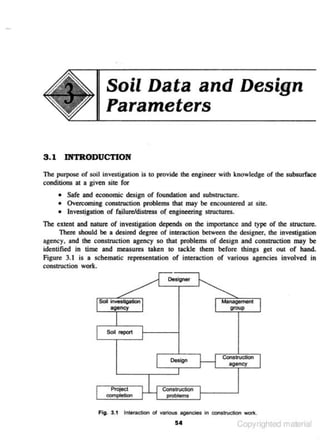
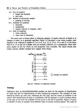
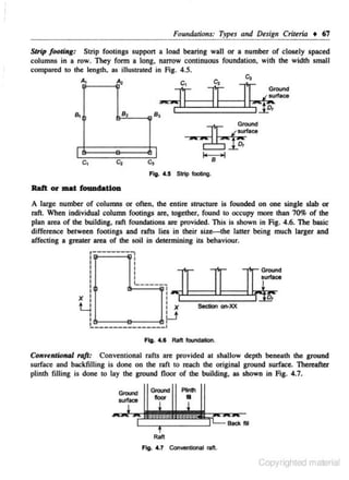
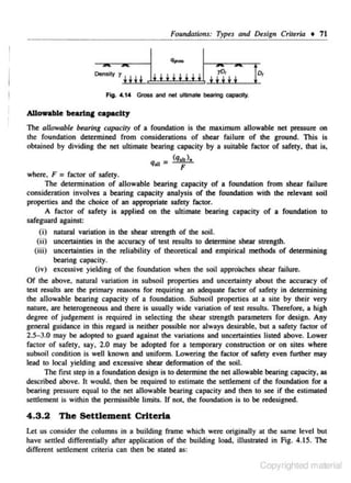
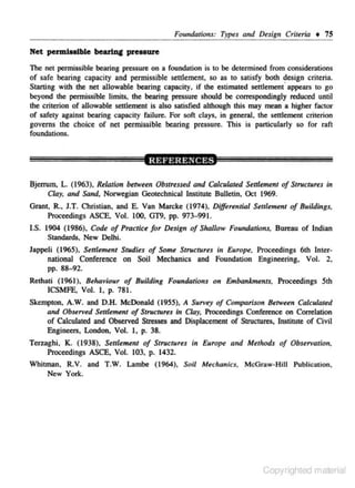
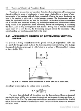
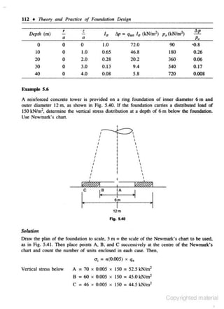
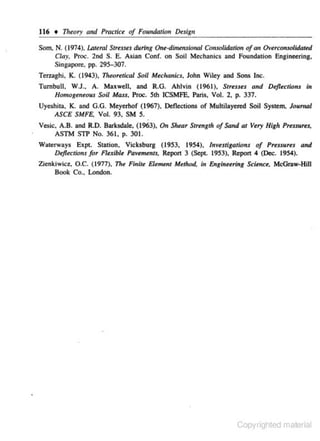
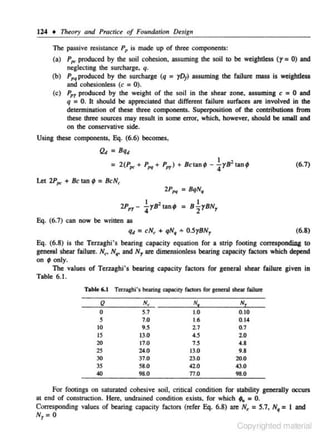
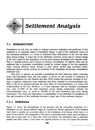
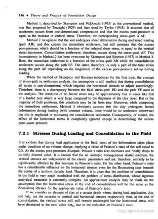
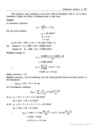
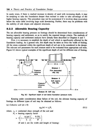
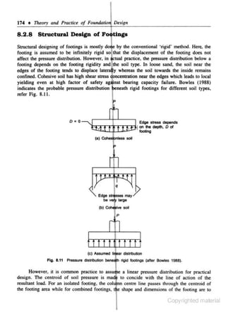
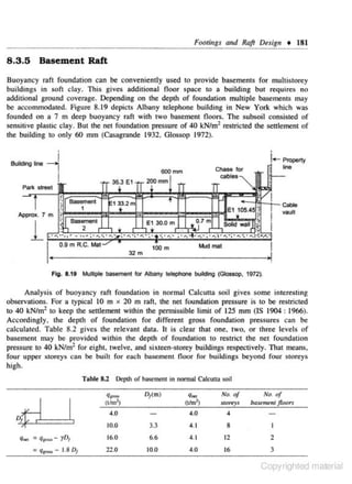
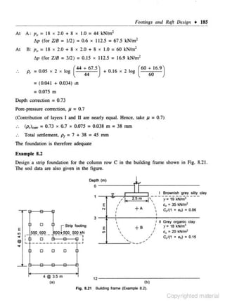
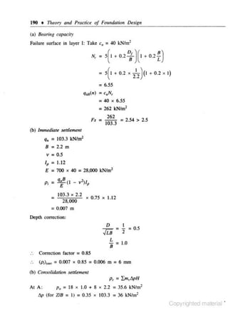
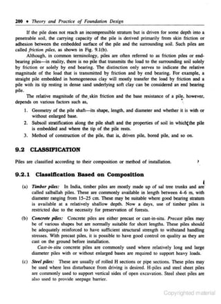
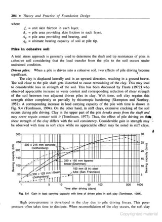
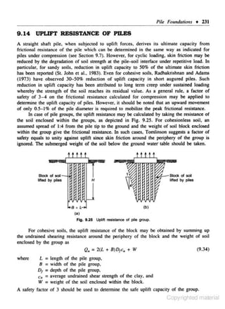
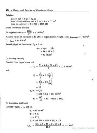
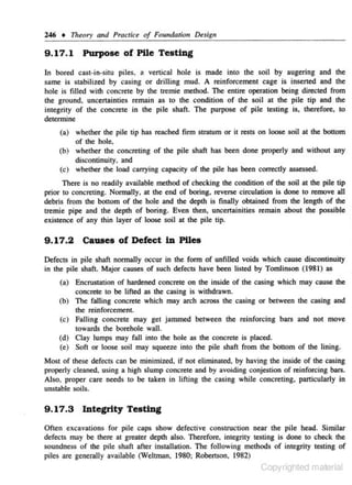
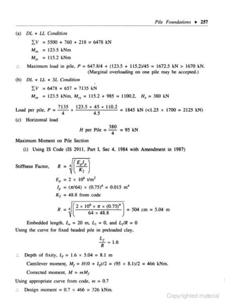
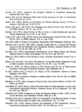
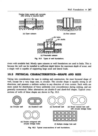
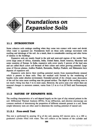
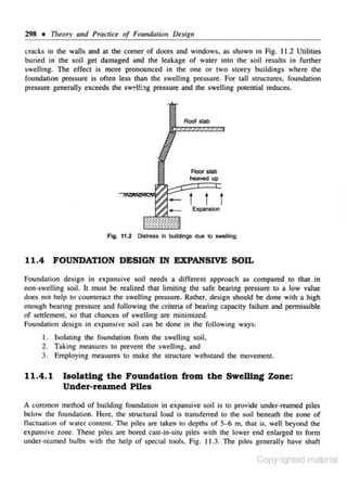
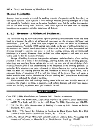
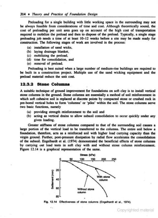
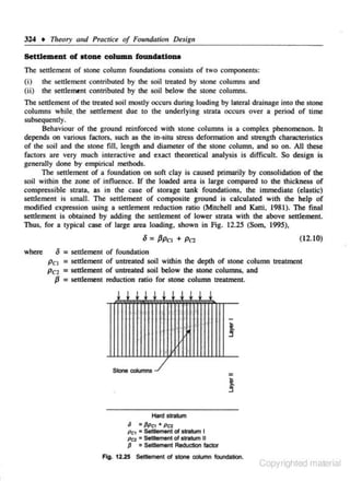
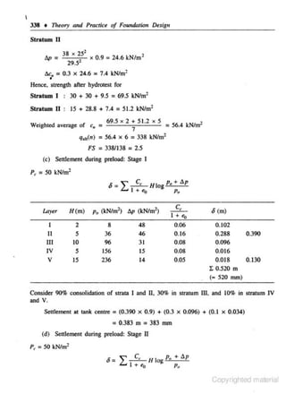
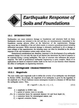
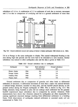
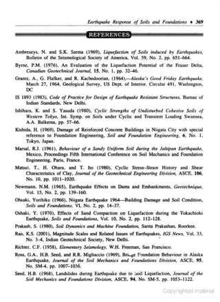
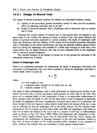
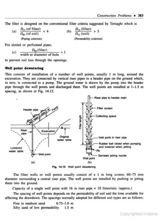
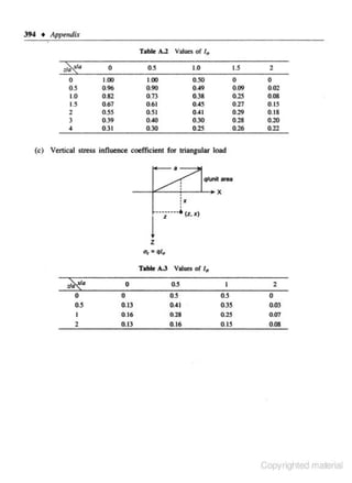
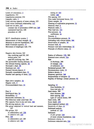
Fig. 1.8
Grai~size
distribution w rve.
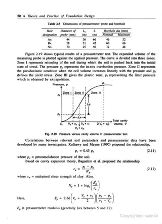
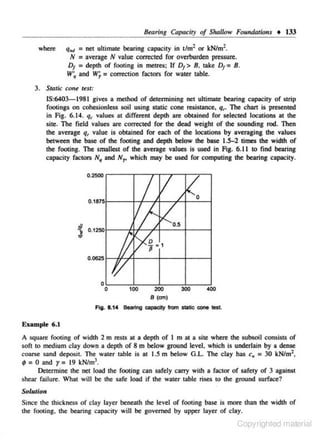
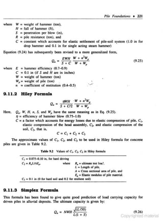
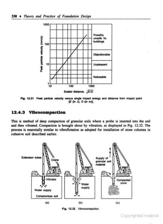
whe.re Dro is the diameter of panjcles correspOnding to 60% fi ner and D 10 is the diameter or
the panicle corresponding to 10% finer. The gradation of soil is detennined by the following
criteria:
c11 = l
Uniform soil
Poorly-graded soil
I < c. < 4
c. > 4
Well-graded soil
It must be considered, howeve,r. that the pilrtic1e size alone is not an adequate criterion for
the classification of a soil. as the shape or grains and clay fraction may vory widely depending
upon the constituent minerals. More elaborate soil classification systems. making use of the
Auerberg limits. in addition to che particle size distribution. have since been evolved.
The roost comprehensive of lhese systems are the Unified Soil classification system and
the Indian Standard Classification System. The Unified Soil Class(ficotio" System divides the
soil.into coarse-grai ned soil (having more than 50% retained on number 200 sieve) and 6 ne
grained soil (more than 50%. passing through number 200 sieve). Further subdivisions are made
according to gradation for coarse-grained soils and plasticity for fine-grained soils and each soil
type is given a group symbol (Table 1.3). The Indian Standard Classification System (lS 1498)
is simii3C in some respeccs except that the fine-grained soils are divided into three ranges of
Jjquid limit as opposed to only two in the unified soil classification system.
1.6 RELATIVE DENSITY OF GRANULAR SOIL
The engineering properties of grnnular soil primarily depend upon its relative density, grain0
s ize distribution. and shape of grains. The relative density determines the compactness 1
which the solid grains arc assembled in a soil skeleton and is expressed as
enw;- e x 100
emu - C~nin
(1 .4)
Copyrighted material

28. Soil as an Engi,eeri11g Material • 7
1.5 SOIL CLASSIFICATION
Density. void ratio. and water content are fundamental soil parameters which help to identify
·and assess-at least qualitatively, the nature of the soil deposit. For example, a high void
ratio of a sandy soU would indicate a loose state of compaction while a clayey soil with high
water content is likely to be more compressible than one with low water content Table 1.2
gives the density, void ratio, and the water content of some common soil deposits.
Table l.l Density, void ratio, and water content of some soils
-
Soil
Gmiogk:
Mexioo City
BW.t dms#y
(8/<c)
9.0
1.6
0.7
0.4
1.3
1.0
1.8
1.9
2.0
1.7
350
o.s
2.0
30
2. 1
0.8
1.0
1.5
80
2.0
30
1.9
38
Volcanic
Eslultrine
Marine
Glacio!
Alluvlal
AlluvW
Marine
Marine
Morine
Shd lhav~n clay. En~and
London Clay. Sdsee
Boulder Clay. England
Nonnal Calcutta CJay (UJ>Pef)
Nonnal Colcuua Clay (Lower)
Bangkok Cwy (Soft)
B:;mgkok Clay (Still)
Norwegian Quick CWy
WaJ~I'
Void
m1io
contmt (Sf!)
60
35
20
so
Soil consisJs of solid grains that have various sizes ranging from coarse grained
particles such as boulder. gravel and sand down to the fine g.rajned particle$ like, siJt and
clay. The grains are classified according to their sizes. The most common system of
classification is the M.I.T. system as illustrated in Fig. 1.7.
2.0
CoMU
0.6
0.06
0.2
Medium
Sand
Fine
0.006
0.02
Coarse
Medium
0.002
Flnt
$lit
0.0006
eo.roe
.
.
00002
Medium
Flnt
(co/IOhJIII)
Clay
Fig. 1.7 M.I.T. dassifk:ation system.
Natural soil generally consists of mixture of several groups and the soil, in such cases,
is named after the principal constituent present. For example. a soil that is predominantly
clay but also contains some silt is called silty clay.
The grain-size distribution of a soil is best represented by the grain-size distribution
curves. refer Fig. 1.8. The shape of the curve indicates whether the soil is uniform or poorly
graded. or well-graded.
llte unifonnily coefficient of the soil is defined as
D
c., = !:12.
D,o
( 1.3)
Copyrighted material

29. Soil as an Engineering MateriDI • 9
where emu = void ratio in loosest stale
emiD = void ratio in densest state
e = in-situ void ratio
The properties of granular soil an: also dependent on their particle size distribution, that
is, whether the soil is well-graded or poorly-graded. In well-~ soils, the smaller grains
~ to fill the void$ between the larger grains and thus, malte the soil more compact. The
shape of grains (angular sub-rounded or rounded) may also have some effect on the
propenies of granular soil.
1.7 SOliE SPECIAL
son.
TYPES
Apart from the common soil types that may be identified by the different soil classification
sY1(ems, cenain natum soils are characterized by the properties of their chemical and mineral
constituents. Such soils exhibit characteristic features with regard to their streJigth and
compressibility and need particular care when used to support a foundation.
Or1anic soilJ are those which contain large quantity of organic/vegetable matter in
various stages of decomposition. Natural soils may contain varied percentages of organic
matter and only a small percentage may be sufficient to affect its properties. In organic clay,
vegetable matter is intermixed with the predominant clay mineral while P<Qr consists almost
wholly of vegetable matter. Peat is characterized by high liquid limit and sponzy mucture
with low specific gravity. The top 10-12 m of the normal Calcutta deposit is a common
organic clay of the Bengal basin. A thin layer of peat is often encountered in this depoait at
many locations as shown in Fig. 1.9.
Dosa1ption ol strata
II Glwy/doltl -
silty day, ~ lilt -
semi·
2...
55
12
28
2.5
0.005
lilly day will calcareous
..-..s
10
30
60
25
8.0
0.002
20
38
20
30
4.5
~
25
65
25
10.0
~-pieooa
Ill Bluilll -
IV -.ysllowioh brown sandy slltlallty tine
sand with OCCISk»naa tenses of brQ'M'I and
grey silty day
V Moltled - - silly etay wl1h lomlnallono
-
0.001
wi1h rusty brown spots
VI Brown.1igllt brown lilly 11M lo medium sand
' >> 4(Y
Fig. 1.8 Notmal Colc:ulla ~
Copyrighted material

30. 10 • Theory and Praclice of Foundation DeJ·ign
Expamive soils are found in many pans of India, Africa, and the middle-east. The
black cotton soils of India and Africa are lhe most common types of expansive clays. These
soils have high expansive potential because of the predominant presence of montmorillonite
minerals. They are apparently stiff when dry but undergo swelling when saturated with
water. e.g .• due to seasonal fluctuation of ground water table. The Atterberg limits along
with the percentage of solid particles less than 0.001 mrn is taken as criteria for identification
and classification of the expansive soils. Table 1.4 gives the classification of expansive clays.
Table 1.4 Classification of expansive clays
IJ,
of Panicl~s
f*rllum
Jndu r~sl Data
Pkulicily
ind<x ('If>)
Probabl~ o:pa~rsion.
Shri>Wge
limit (CJ,)
0.001 mm
Dtgrtt of
apaJUiolt
S41tlrvttd cond;IIOII)
28
20-31
13- 23
3S
II
2S-41
7-12
IS-41
IS
1.8
undtr prtuure of
0.07 kg/cm2 (Dry 10
18
10-16
IS
30
20-30
10-20
10
Vesy hish
Hlsh
Low
Low
GROUNDWATER
The water which is available below the ground surface is termed as groundwatu or
subsurface water. Practically all ground water originates from the surface water. The process
by which the s~rface water infiltrates into the ground surface and percolates deep into the
ground is termed as natural ruluJrge and artificial recharge. Main sources of natural
recharge of groundwater include precipitation, rivers, lakes, and other natural water bodies.
Artificial recharge of groundwater occurs from excess irrigation, seepage from canals,
leakage from reservoirs or tanks, or from water purposely applied on the ground surface to
augment groundwater storage. Water from any of these sources infiltrates into the ground and
percolates downwards under the action of gravity through soil pores and, rock crevices until
further movement is prevented by an impermeable stratum. It is then stored as groundwater.
The groundwater exposed to atmospheric pressure beneath the ground surface constitutes the
wat~r table. Water table rises and falls based on the amount of precipitation, the rate of
withdrawal or recharge. and climatic conditions. Groundwater held by the geolog.ical
formation is. however, not static but moves slowly in the lateraJ ctirecdon towards some point
of escape and appear as springs, infiltration galleries or wells, or reappears to join the river,
or lake. or the sea.
1.8 . 1 Types of Water-bearing Formations
Groundwater occurs in most geological formations, of whjch the most important ones are
aquifers. An aquifer is defined as a geological formation that permits storage as well as
transmission of water through it. Thus. an aquifer contains saturated soil which yields
si.gnificanl quantity of water to wells and springs. Sands and gra.vels a.re typical examples of
formations which serve as aquifers.
Copyrighted material

31. Soli as an Eugiuttrlng Mnttriol • II
Other geological form.ations include aquiclude, aquitard. and aquifuge. An aquiclude
may be defined as a geological format.ion of relatively impermeable material which permiiS
storage of water but is not capable of transmitting it easily. Thus. an aquiclude contains.
saturated soil which does not yield appreciable quantities of water to wells. Clay is an
example of such a formation.
An aquitard is defined as a geologic formation of poorly permeable or semipervious
materiaJ which permits storage of water but does not yield water freely to wells. However, it
may transmit appreciable quantity of water to or from adjacent aquifers. A sufficiently thick
aquitard may constitute an imponant groundwater storage zone. A formation of sandy clay
belongs to this category.
An aquifuge is a geological formation of relatively impermeable material which neither
contains nor transmits water, for exampJe, solid rocks.
1.8.2 Di'rialon of Subeurface Water
As shown in Fig. 1.10, subsurface water can be divided into the following zones:
(a)
(b)
(c)
(d)
Soil-water zone
Intermediate zone
Capillary zone, and
Zone of saturation
!
Ground aurfaca o
~- """'
ln~a1e
zone
!
Cooilary
zone
f
I'
Soil water
Pellicular and
grv....tional
water
cap111ary
wale<
Wolef
.:le
1-
Ground water
1lmpermeoble
FJg. 1.10 Zones of subsutface water.
Soil-water zone
The soil- water zone extends from the ground surface to the major root zone. The soil in this
zone becomeS saturated either during irrigation or rainfall. The water in the soil- water zone
is gradually depleted by evaporation from within the soil and by transpiration by vegetal
growth on the ground surface and if it is not R:plenished. the water content may be reduced
to such an extent that only thin fi1m of moisture known as hygroscopic warer remains
adsorbed on the surface of the soil particles.
Copyrighted material

32. 12 • Th.ory and Practice of Foundntion D.sign
IAtermedlate zone
1be intermediate zone occupies the space between the lowe.r edge of soli-water zone and
upper limit of the capillary zone. This zone usually contains static water which is held by
molecular and surface tension forces in the form of hygroscopic and capillary water.
Temporarily. though. this zone may also contain some excess water which moves downward
as gravitational water. The thickness of this zone may vary from zero when the water table is
high to more than 100 m under deep water table conditions.
Capillary zone
The capillary zone extends from the water table upto the limit of capillary rise of water. In
this case, the pore space may be considered to represent a capillary and hence, just above the
water table almost all pores contain capillary water.
Zoae of oaturattou
In the zone of saturation, all the interstices are filled wi!f! water under hydrostatic pressure.
The zone of saturation is bounded at the top either by the ground water table or an overlying
impermeable stratum, and stntches upto underlying impermeable strata (or bed rock).
Generally, all soils below ground water table are fully satunoted.
1.9
ENG~G
PROPERTIES OF SOU.
1.9 .1" PermeabWty
The flow of water through the pores of a soil under a pressure gradient or under a
differential head is a common engineering phenomenon. ~epage of water through earth
dams and consolidation of clay under a building foundation are some instances where
percolation of water through the soil plays an imponant role on the performance of the
foundalion. The ease with which water can flow through a soil, called permeability, is
therefore. of fundamental importance in soil mechanics.
Ducy'alaw
Darcy' s law which governs the flow of fluid through porous media is also found to be
applicable to soils when now is due to a combination of pressure and positional gradient.
With the exception of flow through coarse gnovels, the flow of water through soils is
streamiined, and can be expressed as:
v = ki
( 1.5)
where.
"' = average rate of now of water in unit time.
i = hydraulic gradient. i.e., head loss per unit length of soil measured in the direction
of flow. and
k = coefficient of penneability of the soil.
Copyrighted material

33. Scil as an Engineering MateriiJl • 13
*
For any given soil, depends on the porosity of the soil. the struCtural amngement of
panicles. the size of panicles. the propenies of pore fluid (e.g. density and viscosity) ciA:.
(Taylor 1948). The temperature of the pore fluid should theorelically have some effect but
for practical purposes. the variation of k with the range of temperature normally encountered
in the soil is small.
The coefficient of permeabili[)' of a soil can be meuured from the laboratory constant
head test. variable head test. or the field pumping test. In view of the hetrogeneity and nonhomogeneity of natural soi~ field pumping tesiS give a better measure of the permeability of
the soil in the field. Typical values of permeability for different types of soil are p ven in
Table 1.5.
Tillie 1.5 Pameobility of cliff.- !ypes of soil
Soill)p<
Grsvd
C>ane sand
Medium sand
-Fine 5aDCl
Slllysand
Sllllweuta.d clays
lntiCl days
t
t- to-'
tcr•- ur'
tO"'-to-'
tcr'-tcr'
to-'- tcr'
tcr'-tcr'
Oood
Poor
Very poo<
Darcy's Jaw is valid only for laminar flow. Since Reynolds number serves as a criterion to
distinguish between laminar and turbulent flow. the same may be employed to establish the
limit up<o which Darcy's law holds good. Reynolds number for this case Is expressed as
.-
R
_ pvd
(1.6)
Jl
where p is mass density of fluid.
v is the discharge veloc-ity. and
Jl is the dynamic viscosity of the Ouid.
Most of the natural groundwater Oow occurs with R, < I and hence. Darcy's law is
valid. However. Darcy's law is not applicable in aquifers containing coarse gravels. rocklills.
and also in the immediate vicinity of wells where the flow may not be laminar due to steep
hydraulic gradients.
1.9.2 The Principle of Effective Stress
In a multi-phase system composed of solids and voids. the behaviour of the material under
applied stresses depends on how total stress is distributed amongst several components in the
soil aggregate, namely the intergranular pressure that acts between the soil grains at their
points of contact and the pore pressure which acts in lhc pore fluid. The normal stress on any
plane is, in general. the sum of two components. namely the stress carried by lhc solid
pan_clcs and the pressure in the Ouid in the void space. The principle of effective stress
i
Copyrighted material

34. 14 • 111eory and Pmctice of Foundation Design
provides a Slltisfactory basis for understanding the deformation and strength characteristics of
a soil under an applied load. This can be simply be stAted as:
(a) The volume change of a soil is controlled not by the total normal stress applied on
the soil, but by the difference between the total normal stress and tile pressure in the
nuid in lhe void space. termed the pore pressure. For an all-round pressure increase.
this can be expressed by the relationship.
6V
--
v
= C (6<7. - 6u)
'
(1.7)
•
where.
6 V/V = volume change per unit volume of soil
6.G,. = change in total normal stress/pressure
6u = change in pore pressure
ct' = compressibility of soil skeleton
This relationship can be illustrated by a simple teSt where a Sllturated soil sample is subjected
to undrained loading followed by drained compression as shown in Fig. 1.11. Not until tilere
is a change of effective stress. is there a change of volume of the soil. This is the primary
cause of long term consolidation se-ttlemenl of foundation on clay. This also explains the
settlement or an area due to ground water tabJ Jowering, either for construction work or for
e
water supply.
Undrained
Total •1ress
l
(A<»)
-·- .-·- .
,pi;
' , 'l<i>·<;r.---·-·
,,...
Streu
! .'
. ,
!•
. , · ... '
r:-
AV
-v
Pore
--
t
......._ • Pressure (.Au)
Time -
........
--
-+
Fill, 1.11 Pnndplo ol olloeiMo ......
(b) The shear strengtil of a soil is determined by tile frictional forces between tile solid
panicles. These are clearly a function of the component of normal stress that is
carried by the solid grains rather than the total nonnal stress on the plane considered.
This ·may be expressed by tile equation.
r = c' + (cr. - u) tan
f
(1.8)
where,
c'
= apparen1 cohesion
(l = angle of shearing resistance
o;. = total normal pressure
u = pore-pressure.
Copyrighted material

35. Soil as an Engineering Matuial • IS
In Eqs. (1.7) and (1.8). lhe tenn (u,- u ) is tenned lhe effective stress and is denoted
by the symbol u', that is,
o' = o - u
( 1.9)
In most engineering problems, the magnitude of total normal stre..c;s can be estimated
from considerations of statics while the magnitude of pore pressure depends on the hydraulic
boundary conditions. Bishop (1955) has shown that the effective stress in a soil can be
related to the intergranular pressure at the points of contact.
For a unit area perpendicular to the plane X- X through a soil rru~ss, the total s tress, u
acting on lhe plane of contact can be divided into two components, (refer Fig. 1.1 2) .
lll l l l l l
u
1
ll l l
"'
1
1
t
Fig. 1.12 EffectlYe stress and lntergranular pressure.
a = o' + u
( 1.10)
where.
u = Pore water pressure and
u• = Effective stress
If a = effective contact area per unit area of the plane and
pressure, then, for a unit area
u
or
x I
= u1 x I + (I -
o-1 = ( U- u) + au
O;
= average intergranular
a)u
(1.1 I)
But a is small (!hough not equal to 0) and hence.
o-1 = (u-
u)
( 1.12)
From Eqs. ( 1.11) and ( 1.12)
o1 = a'
(1.13)
Thus, for practical purposes, effective stress may be considered equal to the intergranular
pressure. the average pressure between the solid gains.
In a natural soil deposit, (refer Fig. 1.13), the total stress at any depth is given by the
overburden pressure at that depth while the pore pressure. in the absence of any artesian
condition, is given by lhe hydrostatic head of water at that deplh. The distribution of total
and effective stress in the soil is shown in Fig. 1.13.
Copyrighted material

36. 16 •
Tlr~ory
and Practlce of Foundntion Design
VertiCal stress
Ground surface
G.~t
__j'___
_
z
A
Depth
Poro
pressure
T-
tlrMS
Fig. 1.13 OltOI>utlon ol lOIII and . - , .... In soils.
Therefore, the vertical total stress at the point A is given by
a. = llt + r<z - :,)
where,
(1.14)
r.
= unit weight of soil within depth lt
r = unit weight of soil below deplh lt
The pore water p.essure
u
= r.<z - l t )
(1.1~)
whete Yw = unit weight of water.
Hence, the effective stress at A is given by
a; = Ytlt + y(z - :,) -
=
when:
r' = submerged density
ll t
r.<z - :,)
+ y '(t - : ,)
(1.16)
of soil below water table
1.9.3 Pore-preuure lD SoU due to Applied Load
The application of structural load causes an incn:ase in the total stresses in the ground, the
magnitudes of which can be delennined from the theory of elasticity. If the subsoil consists
of clay of low permeability and construction is sufficieo~y rapid, these changes in total stress
occur under conditions of no volume change and are associated with simultaneous
development of excess pore water pressure.
The concept of pore pressure coefficient is utilized to obtain a clear picture of how the
po"'"pn:ssure in a soil n:sponds to diffen:nt combinations of applied stress (Skempton 1954).
This concept not only explains the relationship between different types of triaxial test, but
also provides a basis for estimating the ll}ignitude of pore-pressure to be encountered in
practical problems.
Copyrighted material

37. SoU as an Enginuring Martrial • 17
Skempton (1954) expressed the change of pore-pressure in a soil under axi-symmetric
stress changes in terms of two empirical parameters A and 8 where
( 1.17)
where.
Au = change in pore-pressure
Aa1 = change in total vertical pressure
Aa3 = change in total lateral pressure
A and B = pore-pressure parameters
By putting Aa3 and (Aq1 - Aa3) equal to zero successively, it can be shown that the
parameters B and A represent the effect of the aJI round stress increase and the deviatoric
stress increase respectively on the pore-pressure developed in a soil element. Accordingly,
Au = B·Aa3
when Aa1
-
Aa3 = 0
when Aa3 = 0
and
( 1.18)
The parameter B depends on the degree of saturation of soil (for fully saturated soil B = 1).
1be parameter A. however, depends upon a number of factors such as srress history of the
soH. stress level. strain level. and so on, the most influential being the stress history. that is.
whether the soil is nonnally consolidated or overconsolidated (Lambe 1962). Table 1.6 gives
typical values of pore-pressure parameter A for different stress history of the soil.
Table 1.6 l'on:·pru$U,. parameter A of differont soil types
VQ/u of A aJ failun
Sensiti~
clay
1.2-2.S
0.7-1.2
Normally consolidated clay
0'erconsolidakd day
Heavily overconsolidatcd cLay
1.9 .4
0.~.7
-0.~.0
Shear Strength of SoU.
The shear strength of a soil under any given condition of drainage is defined as the maximum
shear stress which the soil can withstand. When a structure is erected on a soil, the soil elements
beneath the foundation are subjected to increased shear stresses. The capacity of the foundation
to bear load is a function or the shear strength of the soil. The maximum shear stress a soil can
withstand depends to an appreciable extent on the manner of loading and the boundary
conditions. A soil specimen does not. therefore. have a unique shear strength and it depends on
factOrs such as rote of sttain, drainage condition, and size of sample.
The faj lure. criterion most commonly used for defining the shear strength of a sqil
along a plane is expressed by the Mohr-Coulomb equation. as illustrated in Fig. 1.14,
r = c + a.
tan;
(1.19)
where
c is lhe cohesion intercept.
a" is the normal pressure on the plane considered, and
; is the angle or shearing resistance
Copyrighted material

38. 18 • Theory and Practice of Foundalio, DeJign
~
.!!
•
"
•
•
eli
4
'
c
Normal stress
Ffg:. 1.14 Mohr-Coulomb faJiure criterion.
In Eq. (1.19). the shear strength parameters c and 9 for any panicular soil depend on several
factors, the most important being the condition of drainage. Therefore, Eq. (1.19) expressed
in tenns of the total normal s-tress on the plane considered may be used to study the shear
behaviour of soiJ under undrained condition. A more general expression may be written in
terms of effective stress (Bishop 19SS) as:
r: c' + (a. - u )
9'
-r' = c' + a' tanf'
or
where c' and
tan
(1.20)
f are the shear strength parameters in terms of effective stress.
lleuuremeut of ahear IOtteueth
While the Vane shear test (Cadling and Odenstnd 1950) or the Pressuremcter test (Menard
1956, 1969) may be used to determine the undrained shear strength or soils in the field, the
shear behaviour of soils is best understood from the laboratory triaxial test. figure 1.15
Luclte chamber
Chamber fluid
Sol
specimen
To drainage and!Of'
pcwe watet preuure
Copyrighted material

39. Soil
41
an Enginuri.ng
Mat~n·al
+ 19
shows triaxial test set-up. Here, a cylindrical soil specimen is enclosed in a thin rubber
membrane with rigid caps at top and bouom. The soiJ is placed inside a triax.ial cell which is
then filled with water. Pressure is applied to the specimen through water and deviator stress
is applied through the end caps until lhe specimen fails in compression. Drainage or waler
from the pores or the soil may be conttolled through suitable valves at the base or lhe
triaxiaJ ceiJ. If required~ volume change and/or pore water pressure can be measured. Tile
details of the triaxial apparatus and various tests that can be performed with it have been
described by Bishop and Henkel (1962).
Typeo of trlulaJ teot
There are, in general, three conditions of drainage under which the triaxial lest is performed,
namely unconsolidaled undrained (UU). consolidaled undrained (CU), and consolidated
drained (CD).
In the unconsolidated undrained (UU) test, dte sample is first subjected to an all round
pressure a3 and !hen to a deviator sttess (a 1 - a 3) under undrained condition. The deviator
stress is applied rapidly-usually at a rate of strain of 1-2% per minute, ana failure is
achieved in 10:.20 minutes. For saturated soil, lhe Mohr envelope remains hOriZ9ntal giving
;, = 0. The shear strength obtained from lhe UU test is called lhe undrained shear strtntrh
or the soil c., see Fig. 1.16. The sbear sttength obtained from lhe UU lest is used in the
study of bearing capacity of foundations on clay or in the rapid construction of embankments
on clay. The unconfined compression test is a special case or UU test, where no confining
pressure is applied to the specimen prior to shear.
She•
Sire»
Total S.b'ess failure
· · - (,•0)
Normal
stress
Fig. 1.1S Unoonsolictated undrai'led (UU) test on sah.nled clay.
In the consolidoled undrained (CU) leS~ the sample is allowed to consolidale under an
all round pres..~ure a3 but no drainage is allowed during shear. If pore pressure is measured
during the test, both the pore pressure parameter A and 8, and the shear strength parameters
c' and , can be determined. Figure 1.17 depicts consolidated undrained (CU) test on
saturated clay. The data from CU test may be used in the analysis of stability for stage
conslruction of embankments on clay.
Copyrighted material

40. 2t •
nu~ory
and Praclice of FoUJuiaticn Design
•. u·
______
... -- ---
~ -~-- --
.
__,_
··7.5"
'
I
u
_.,
Namal -
...
3.01P"q
u_.,. •.o .,,,
."
(lcQicm')
Fig. 1.17 Consolidaled ..-!nod {CU) -
on oalura1ed day.
The consolidated drnined (CD) test diffen from the cOIISOiidated undrained test in the
way that both, the initial all round pressure and the subsequent shear stresses are applied
under fully drnined condition. The test, therefore, gives the shear strength parameteiS of a
soil in terms of effective stress, as given by Fig. 1.18. The results of this test can be used in
the study of long tenn stability problems.
{
L--":!,o,. -,a~.-----~~=;:".:,;4
ai Normal stresS
Fla. 1.11 Consclklaled dtalnod (COl -
r..-
Facton affectmc andral.ned ohear atre..,U. of clay ID-eltu
Different types of triaxial test find their applications in specific field problems but, the most
important strength parameters required for the analysis of foundations on clay are those
obtained from the quick unconsolidated undrained (UU) triaxial test. For saturated clays, this
shear strength is expressed by the undrained cohesion c. · '" should theoretically be zero. if
the soil is fully saturated (Skempton 1948). Therefore, the shear strength of the clay in this
condition may be expressed as
( 1.21)
Although the UU test is easy to perfonn in the laboratory. application of the test data
to field problem has to be done with care. Facton such as anisotropy, rate of shear, sample
size. and so on affect the test results significantly (Skempton and L. Rochelle 1955). For
stiff-fissured c lays, in particular. the shear s tre ngth of the clay mass in the field may be
Copyrighted malerial

41. Soil as an Eng;neering Material • 21
considerably less tlw1 the strength obtained from conventional labonltory tests on small size
samples (Biihop 1966).
Seu!ttnty
Most clays have been found to lose a part of their strength when remoulded. This remoulding
may be caused by physical or mechanical means such as pile driving. However, with time,
the clay may regain this strength either wholly or partly, by a phenomenon known as
thixotropic hanl•ning (Skempton and Northey 1952). From the point of view of sensitivity
towards remoulding, clays may be classified as fol lows (Table 1.7):
T•ble 1.7 Sens.itivity of cl1ys
(Skempton and Northey 19S2)
Less than 2
2-4
4-8
8-16
16
loscnsitivc
Moderalety sensltivc
Sensitive
Very sensitive
Quiet clays
SensHivity. in chis context. is defined as lbe ratio of tbe undrained shear strength of lhe
undisturbed soil to that of the fully remoulded soil.
1.9 .5 ConsoUdatlon
The gradual squeezing out of water from the pore space of a soil skeleton under the
influence of externally awUed load or gravity is called co•solidation. The process results in
a net change in volume of the soil and is time-dependent
When an element of soil is subjected to an increase of rotal suess under undrained
condition, the pressure is distributed among the solid grains and water depending on the
rclarive comprcssibililies of the two phases and lbeir boundary conditions. For a confined
saturated clay- water system with no drainage, the compressibility of the mineral skeleton is
so large compared to that of water alone that virtually all the applied pre&&ure is transmitted
as an excess pore water pressure. If drainage is now permitted. the resulting hydraulic
gradient initiates a flow of water out of the clay and the soil consolidates. There is a
consequent transfer of the applied load from the water 10 the mineral skeleton.
The mechanism of consolidation and the factOI'S that govern lhe process of consolidation
of c layey soils are studied experimentally in the laboratory in the consolidation test or the
oedometer test The arrangement for nedometer test is shown in Fig. 1.19. A sample. usually
76 mm dia x 20 mm thick, is enclosed in a mel2l ring and sandwiched between two porous
stones placed at top and bottom. A load is awlied to the sample through the porous stones
using a lever anangemenl. As the sample consolidates., thickness of the sample decreases.
Being laterally confined within the metal ring, the sample is prevented from expanding
laterally and the entire volume change takes place in the venical direction. The flow is,
therefore, one dimensional and the tate of consolidation is governed by the permeability of
Copyrighted material

42. l l • T1reory and Pracrict of Foundation Dt.sign
the soil in the vertical direction only. However, consolidation is not always oneoodimensional
in rhe field and the consolidation test as performed in the laboratory represents the field
condition only under certain boundary conditions.
Olal
-1----..jf+- Po"'"s sle>ne
Pre.eure-vol4 ratio relatloaolllpe
111e change of volume of a sample as measured in the consolidation test is a function of
increment in applied stress and is generally expressed in tenns of the pressure-void ratio
relationship of the type shown in Fig. 1.20. For a normally consolidated soil, this
relationship is found to be linear on a semi-log ploL
..
~ .... 0.
'
1!
>
~ ... ~
--·----~-----
.,:
p,,
... ;-
6P
:
Po:
,P,
Pressure
Pressure
Fig. 1.20 p,_...-wlcl ratio retotionohlp.
p, :
(log
scate)
The coefficient of volume decrease is defined as the volumetric strain per unit increase of
effective pressure and this can be expressed. in terms of void ra6o, as
m, =
.
de
I
dp 1 +
•o
(1.22)
where.
t.o = in.itia.l
void ratio for dte s.tress increment considered.
Copyrighted material

43. Soil as an Engineering Material • 23
For the linear void ratio versus effective stress relationship on the semi-log plot, the
compressibility of the soil is gjven by the compression index. C, defined as
de
d(logp)
c, :
dV
and
-
v
:
c,
I+~
(1.23)
log 12.
(1.24)
Po
The compressibility of a soil is a measure of its consistency. The greater 1he
compressibility, the softer is the soil and vice versa. Again. the compressibility of a soil is
not a constant propeny. lt decreases with increasing effeetive stress, as is evident from the
decreasing slope of the pressure-void ratio relationship with increasing pressure. But for the
range of stresses usually encountered in practice~ Table I .8 gives one dimensional
compressibility of some representative clays.
Table 1.8 <Joe.<timemioo.al compmsibifity of some cl.tys
Szrtn His.tory
Qay
Goopon Clay. England
Shellhavm Clay
Nonnal Calcuua Clay
Cochin Morine Clay
Brown London Clay
Blue London Clay
Non&.~ Calcuua Clay
Nonnally Consolidated
Over Consolidated
m. (m2/lcN)
C,AI + •ol
0.0015
0.0025
0.0005
0.0006
0.017
0.010
0.1~.20
0.20
o.os
(desiccaled)
(Dau from St cmptoa aDd Bitbop (19S4).
Onammcr (1976) and Author's fikl)
!'formally eonoolldated aDd onrcoaooJJdated cJaya
Let us consider an element of soH during deposition under water, Fig. 1.21. As more and
more soil is deposited on lhe elemen~ the overburden pressure on the element increases and
its void ratio decreases along the curve AB. When the maximum height of deposition~ H,. is
reached. the pressure increases to Pe and the void ratio decreases to ~r The soil·anywhere on
the curve AB is called nomrally consolidated, to indicate thai it has never in its past, been
subjected to a pressure grester than that corresponding to the curve AB. Marine clays and
alluvial soils of India are typical examples of nonnally consolidated clays.
Ground
Erosion
'---~--~-- log
p
Fig. 1.21
Po
stresses in en
etemenl soil below ground surface.
p,
p
Copyrighted material

44. 24
t
Theory Olld Practice of Founda1io11 Design
Now, if some pan of the overburden is removed by, say. erosion and the remaining height of
deposition is only H. conuponding to which the pressure is Po- the e lement of soil will
undergo swelling and the void ratio will increase to e. This means that the soil in its past has
been subjected to a pressure greater than that exists now. Many <:lays and clay shales. for
example, London clay and Bearpaw shale, are heavily ovcrconsolidated in nature. The
strength and deformation characteristics of a soil depend to a large extent on it being
normally consolidated or overconsolidated. Soft clays are normaJiy consolidated and their
behaviour diffe.rs from overconsolidated c lays and clay shales. Structures founded on
normally consolidated clays. in general, experience much more settlement than those founded
on overconsolidated clays.
Although erosion of overburden has been identified as one of the causes of
overconsolidation. many residual and alluvial soils near the ground surface are rendered over..
consolidated by desiccation. Alternate wetting and drying due to seasonal Ouctuation of water
table and changes of temperature intrOduce capillary forces in the soil and the latter develops
a pseudo overconsolidation effect. This results in increased strength and decreased
compressibility of the soil. Depending on the severity of changes during desiccation, the over
consolidation effect may be quite appreciable. Most residual soils of India and occasionally
the alluvial soils near the ground surface appear overconsolidatcd due to desiccation.
Rate of eo.....Uclatl on
The rate of consolidation of clayey soils is governed by the theory of one-dimensional
consolidation (Terzaghi 1923), as shown in Fig. 1.22:
....,.
Z Ground
z•
z
H - --- --
=0
(b)
(a)
Ftg. 1.22 On&-<Jimenslonal oon1011da1ion.
The one-dimensional consolidation rate is expressed as
2
ou ; - k ou
St r.m., sr.z
(1.2S)
where u is ihe pore pressure at a depth z from the free drainage surface, at a time 1 after the
pressure increment; and k and m,. are the permeability and compressibility of the soil for a
particular pressure increment. Both k and m,, may vary with pressure but their ratio remains
Copyrighted material

45. Soil •s an Engintering Mauritll + 25
approximately constant (Skempton and Bishop 1954). Conse<juently, Eq. (1.25) may be
writte.n as.
liu ~ C li u
lit
• liz'
1
(1.26)
where C" is defined as the coefficient of consolidation.
Solving Eq. (1.26) for the appropriate boundary conditions, we get the distribution of
excess pore pressure with depth at a given time t as shown in Fig. 1.22(b). Then, integrating
the area of the pore pressure dissipation diagram at a given time and expressing it as a ratio
of the initial pore pressure diagram, we get the average degree of comolidation, U of the soil
as a function of the time factor T~ Thus, the degree of consolidation, U can be conveniently
expressed as,
( 1.27)
U = /(T,)
where.
( 1.28)
and H = length of the drainage path, to be taken as full depth of c lay when drainage is from
one end and half the depth of clay when drainage is from both ends.
The coefficient of consolidation is governed primarily by the size and nature of
particles as reflected by tbe water content or whether the soil is nonnally consolidated or
overconsolidated. C" is determined from laboratory consolidation test by curve fitting
methods (Taylor I 948). The relationship between the U and T. for tbe most common
boundary conditions of single or two-way drainage is ploned in Fig. 1.23.
1.0
Send
0.8
2H =
IT·41
I
Send
H,}H
0
10
Rod<
j+-4u,.j
---
0.2
v
v
...
~- ~~;:,
Sand
/
/
30
50
60
A""rage degree of consolidation, U{%)
70
80
90
This g.ives the C., value for one-dimensional consolidation or small size specimens. U.S.
Department of Navy (1971) proposed nn empirical relationship between C11 and liquid limit
ror determining che field c" for proclical use and lhis is shown in Fig. 1.24.
Copyrighted material

46. l6 • Theory and Practice of Foundation Design
•
'
....
•
•
•
•
".
'
]
~
'
.... '
<5 •
"-<
"
/
'
.
~"
/
Undisturbed samples;
Cv in range or >nrgin ccmpres.sion _
c., in range of rec::ompression lies
aboYe this lower limit
/
'
•
•
['..
•
~
I'..
'-..
' ~lely remouldod.L . . . .
f"-~:t'--~
lies below this Uml
•
.......
•
•
., '"'
LIQuid limit I.L
•
'
.
"'
.......
.. ..
..
,
...
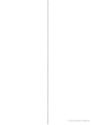
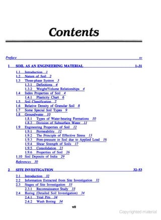
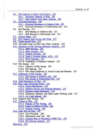
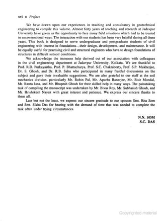
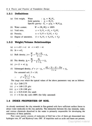
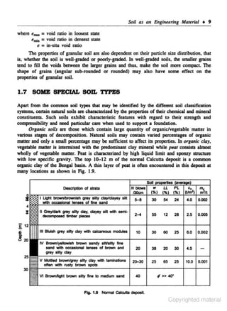
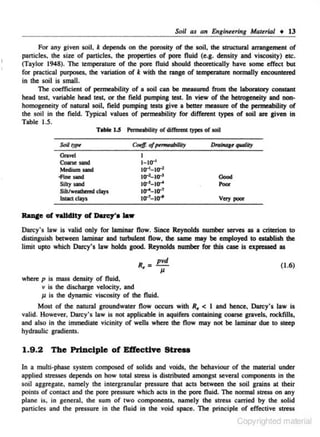
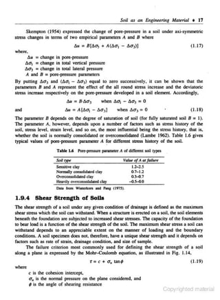
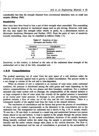
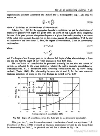
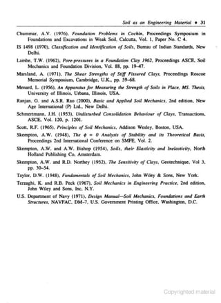
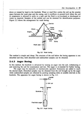
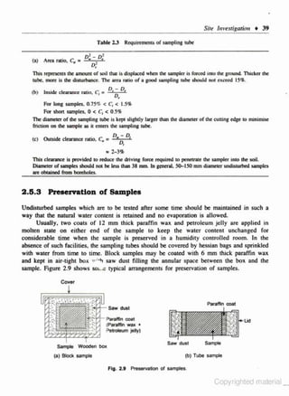
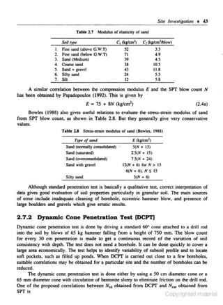
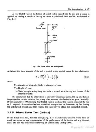
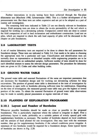
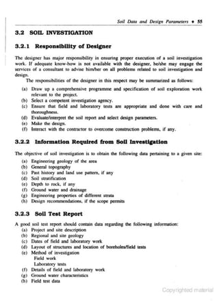
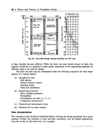
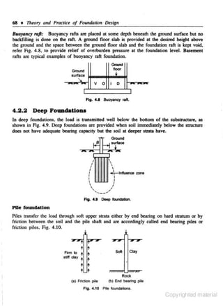
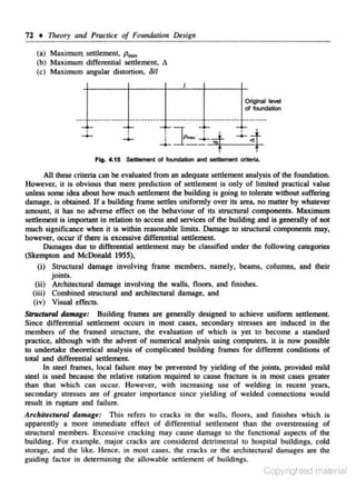
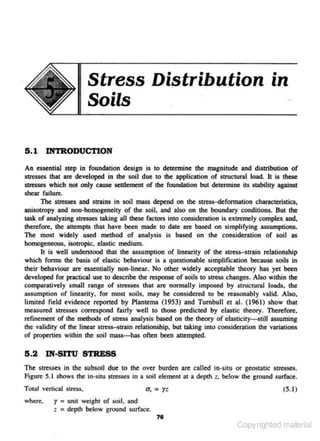
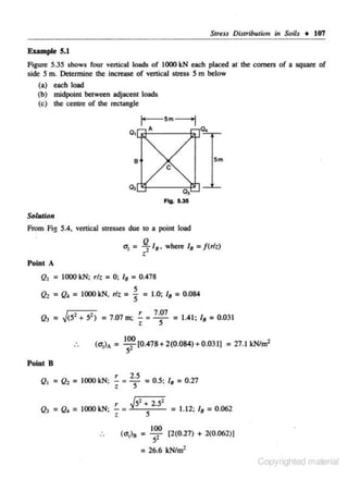
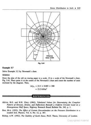
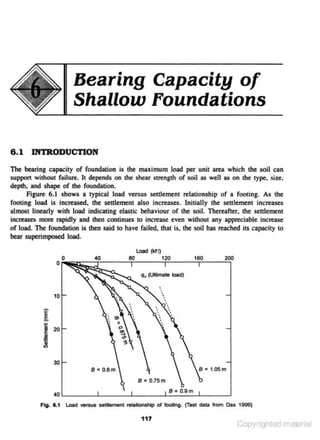
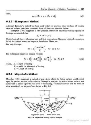
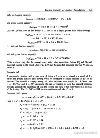
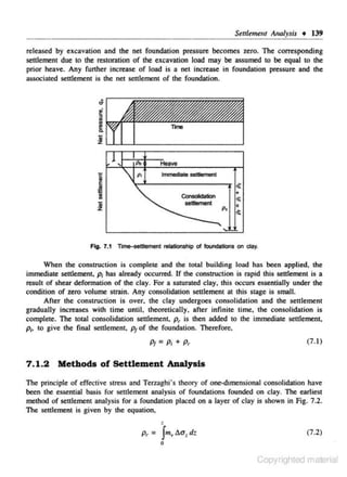
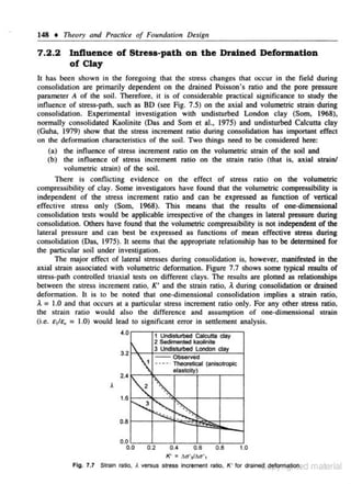
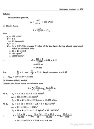
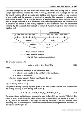
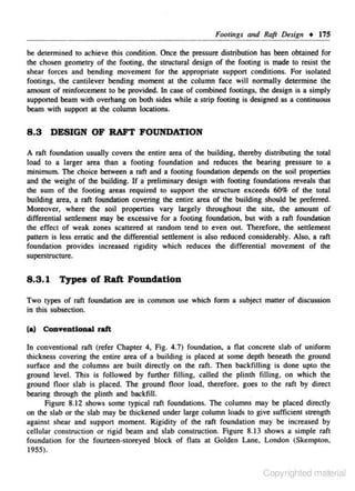
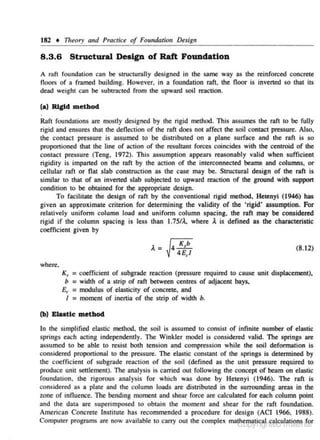
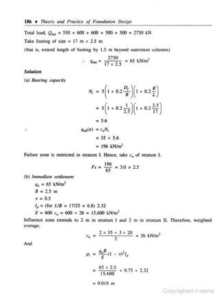
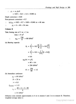
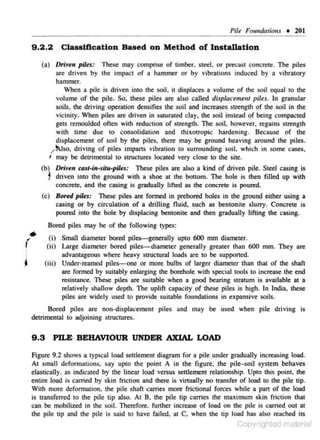
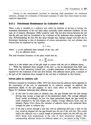
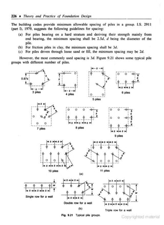
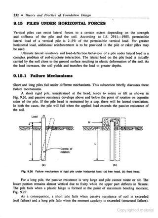
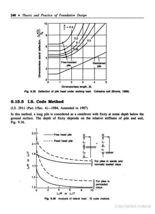
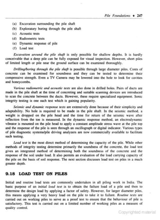
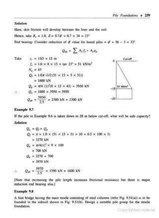
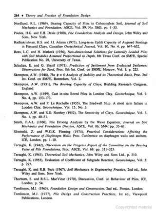
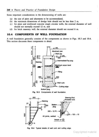
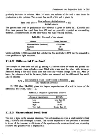
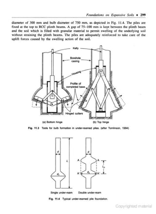
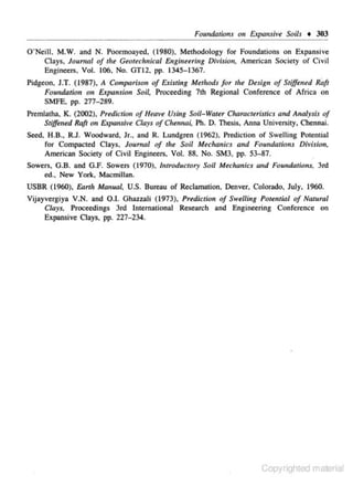
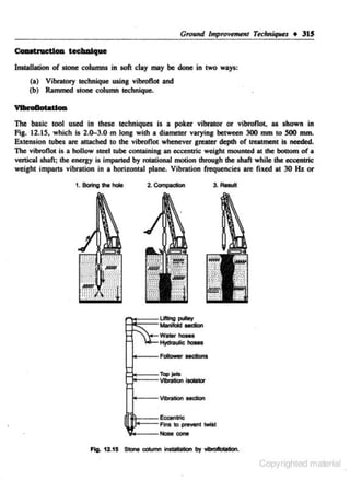
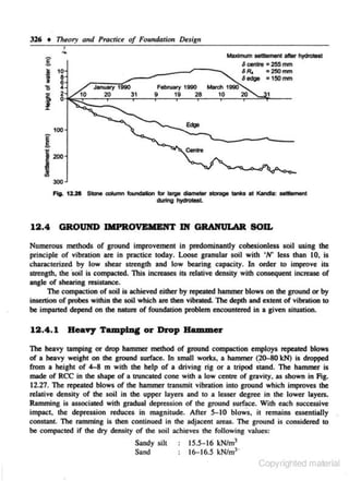
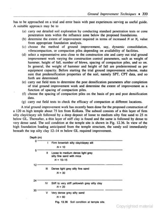
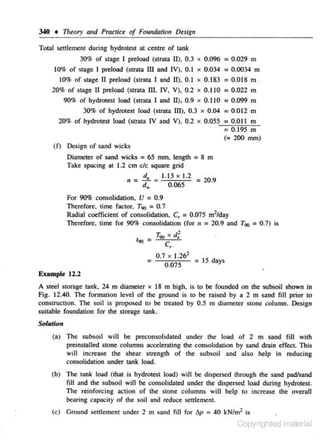
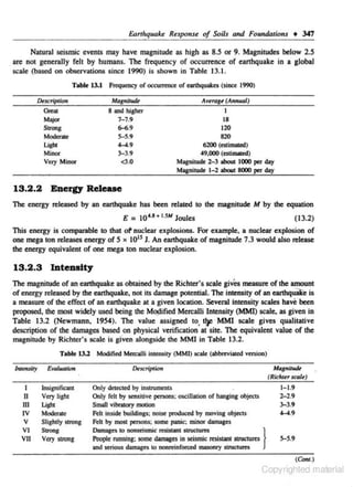
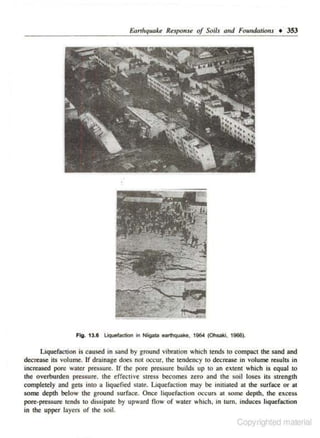
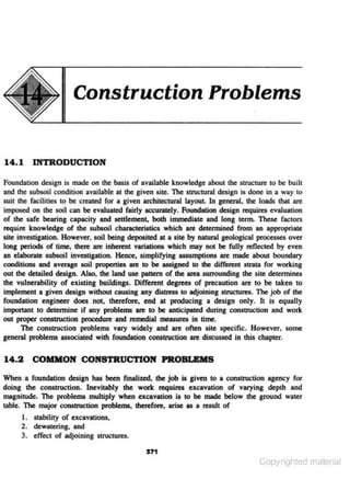
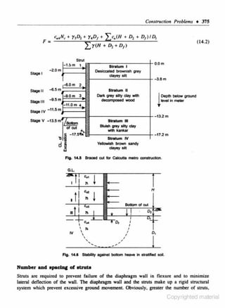
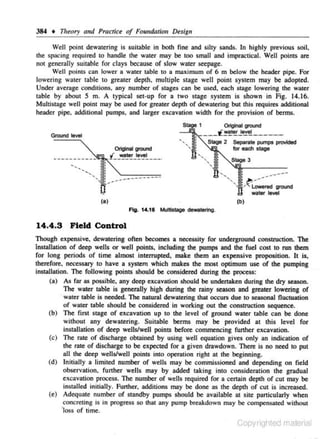
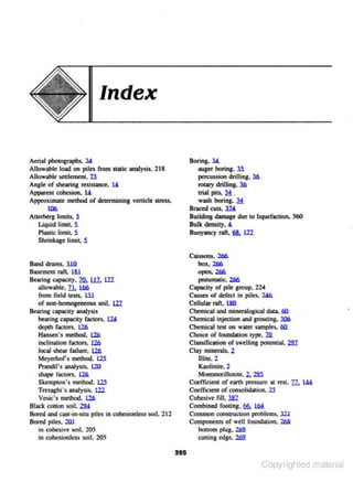
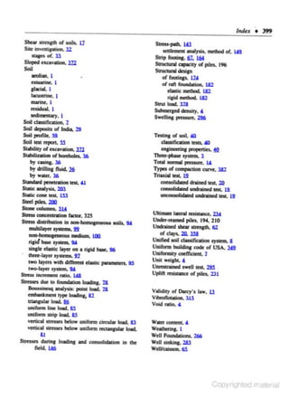
Fig. 1.24 Yal'iation of C., with lquid limit (after U.S. department of Navy (1971)).
1.9.6 Properties of SoU
Coane·p-a.IDecl ooiJa
The relative density of granular soils is measured from in·situ standard penetraticn test. This
test involves counting the number of blows required 10 drive a standard split-spoon sampler to
a depth of 30 em by means of a 65 kg hammer falling from a height of 15 em. An empirical
comlation between standard penetration resistance. N (blows per 30 em), the relative density.
and shear strength of granular soils is shown in Table 1.9 (Terzaghi and Peck 1967).
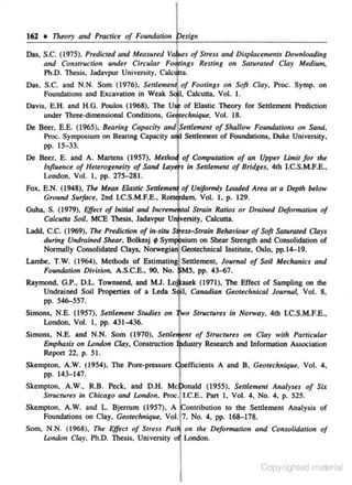
Table 1.9 Relative density of granular soils
(Tcrzoghi and Peck 1967)
Rtldl1tt
dtnsity (%)
0-15
IS-35
JS-65
65-35
7-85
Nott':
N
(Btows/30 em}
().4
4-10
10-30
30-50
so
~values are tO be increased by
Anglt' of shroring
ruislana (f)
u•
Very Loose
28-30"
Loosc
Medium
Dense
Very Omse
30-36'
3~ ) 0
41.
s• for soils containjng less th.an~~~Ytighted material

47. Soil as an £nginuring Matt!rial • 17
•
Pine-grained eoUa
Soils containing clay-size particles and large proportion of silt have low permeability and
their propenies vary wilh the rate of load application. Under undrained condition. their
sttength is derived almost exclusively from cohesion. These soils oflen possess low shear
strength and high compressibility, lhus mal<ing !hem poor foondation materiaL
A cohesive soil is described as ve:ry soft. soft. medium. stiff, and so on according to its
shear s1rength as determined from the unconfined compression test or from !he undrained
uiaxial test. Attempts have also been made to correlate thC standard penetration resistance (as
above) with the shear strength of cohesive soils. Table 1.10 gives the classification of
cohesive soils on !he basis of their shear strength (ferzaghi and Peck 1967).
Table 1.10 Shear $lTCngth of cohesive soils
(l'erughl and Peck 1967)
Undrained $hMt'
<AnsUttncy
strtngth. c.
N
(Blows ptr 30 em)
(lfm:)
~1.25
~2
1.25-2.50
2.5()-S.OO
2-4
Very Son
Son
Medium
Sliff
S.~IO.OO
Very Stiff
10.~20.00
4-8
8-16
16-32
> 20.00
32
Hllld
Stiff clay often possesses cracks and fissures which affect the shear slrCngth of 1 clay
he
mass. These fissures are planes of weakness and an: prone to softening by water. Laboratory
tests on small specimens do not often give lhe propenies of the soils in~·situ (Bishop 1966,
Burland et al. 1966, Man;land 1971).
Elaatlc: parametera
Young's modulus and Poisson's ratio are impOrtant soil parameters thai are required to study
the defonnation behaviour of a soil. When a saturated clay is loaded rapidly. no volume
change of the c lay occurs during loading and Poisson's ratio can be taken as 0.5. When there
is volume change. typical values of Poisson 's ratio may be 1aken as those in Table: 1.11
(Barkan 1962).
Tablt 1.11 Poisson's nuio or di.fferent soils
(Barkan 1962)
Soil f)'Pt
Salurated clay (undrained)
CJ:ay with sand and silt
Un.sawrated clay
Lo<..
Sand
P<'iSJ()n ·s ralio
o.so
0.30-0A2
0.35- 0.40
0.44
0.30-0.35
Copyrighted material

48. 28 • Theory mui Practice of Foundation Design
Young' s modulus of a soil can be determined from the stress-strain relationship
obtained from laboratory triax.ial tests. However, these relationships are highly susceptible to
sampling disturbances and the E value thus obtained is generally much lower than the in-siru
modulus. In ca.iie of homogeneous deposits, detennination of £ by back calculation from field
plate load test gives reliable data. lndirec.t estimate of E can also be made from empirical
relation with the shear strength measured from the unconsolidated undrained triuial lest.
Bj errum (1964), and Bozuzuk and Leonards (1972) suggest the following approximate
correlation:
(1.29)
E = (500 - IOOO)c.
where c., is the undrained shear strength of the clay.
ln·eltu compreselbllity
The pre.ssure versus void ratio relationships of natural clays are vuy sensitive to sampling
disturbanc.e s and the linear e versus Jog p relationship is not always obtained even for a
nonnally consolidated clay. Also, there is a pseudo overconsolidation effect on the sample
because of the removal of in-s itu stresses by sampling. Consequently, e versus )og p
relationship obtained from laboratory consolidation tests on undisturbed samples geniraiJy
takes the shapes as shown in Fig. 1.25. The curves move downwards as the sampling
disturbances are increased. Schmertman (1953) observed that. irrespective of sampling
disturbances. the straight Jine portions of all the curves meet at a void ratio equal to 0.42 ~0•
where e0 is the in-situ void ratio of the sample. Then joining this point with that
corresponding to t 0 and Po (where Po in·situ effective overburden pressure) would give the
virgin consolidation curve. For norma11y consolidated soil, the e.0 -p0 point lies to the right of
the extension of the straight line in the laboratory e versus log p curve while for overconsolidated samples. the point would lie to the left. The field • versus log p relationship for
the overconsolidated range is obtained by drawing a line parallel to the laboratory rebound
curve and the point of intersection of this line with extended straight line of the laboratory
curve would give the pre-consolidation pressure (Fig. 1.25).
=
Void
ratio, e
----
'
••
LabOratory
.,
Po=Pt;
''
-'~~,~ VW'gin ~ression
curve. slope c f:
oonsoCidalion 1
curve
•
---- -- ~-
1
I
I
I
I
'
OA2~;to ------~ -+1
I
I
I
_ _,__;__~ Pressure,
p, P2
p (tog scale}
Fig. 1.25 Laboratory e versus log p relationship.
Copyrighted material

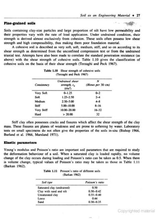
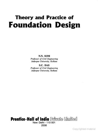
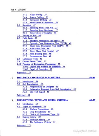
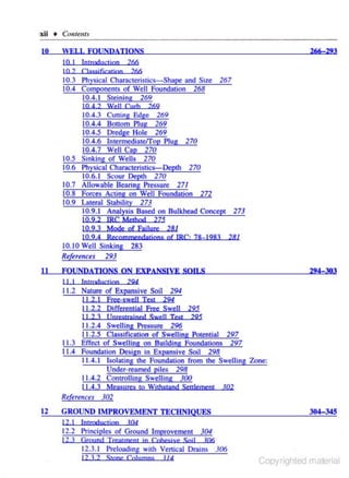
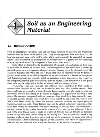
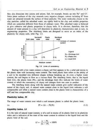
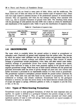
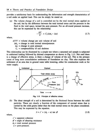
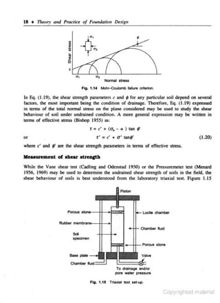
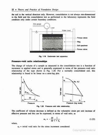
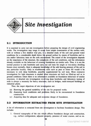
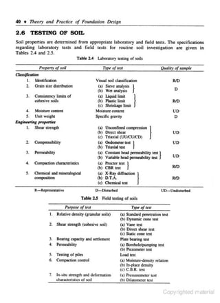
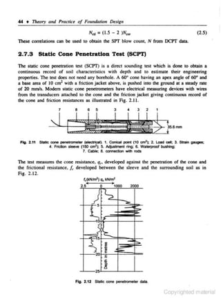
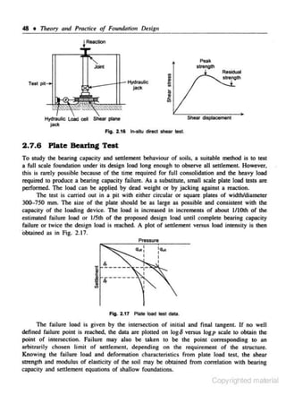
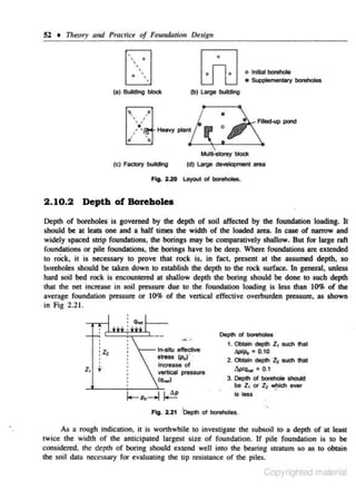
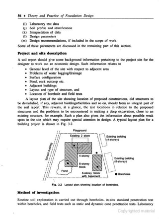
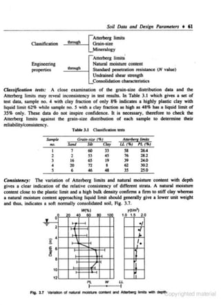
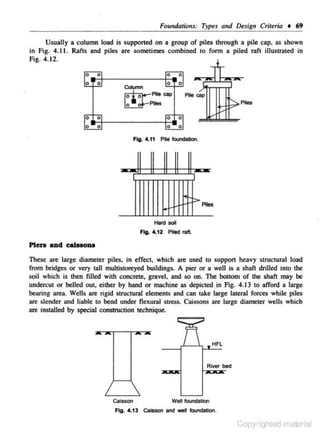
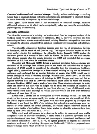
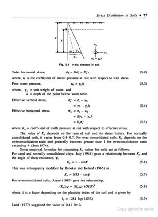
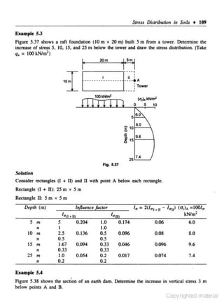
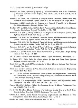
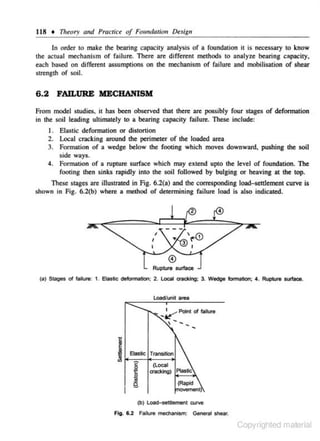
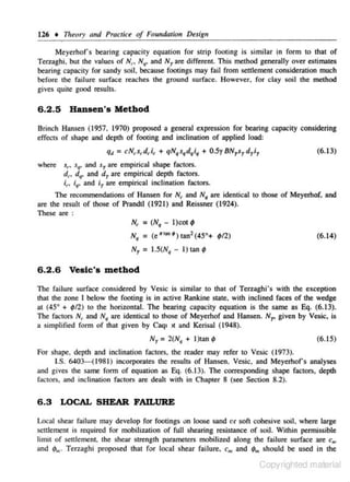
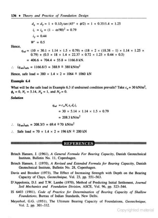
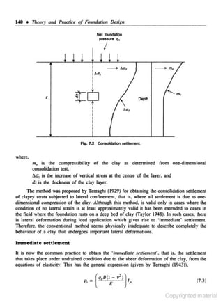
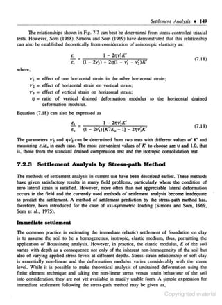
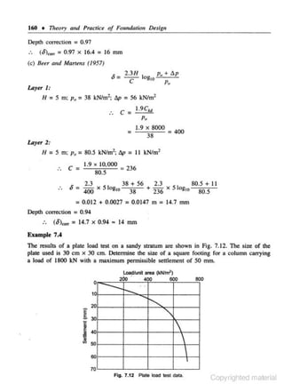
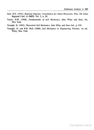
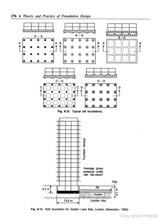
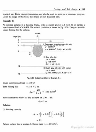
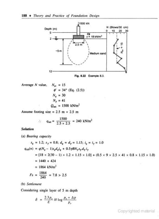
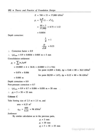
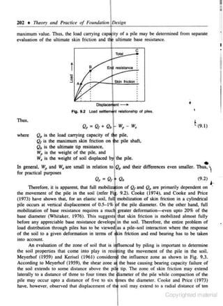
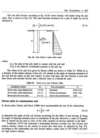
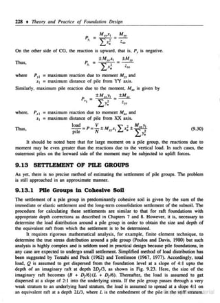
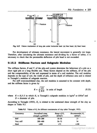
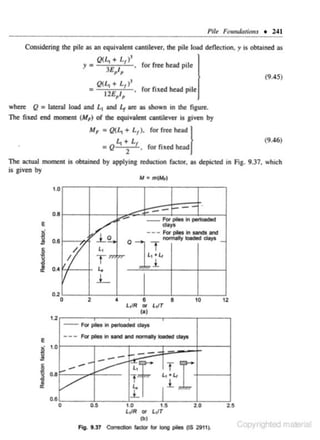
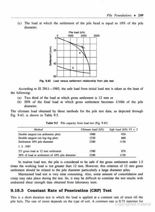
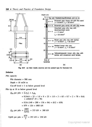
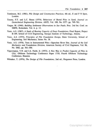
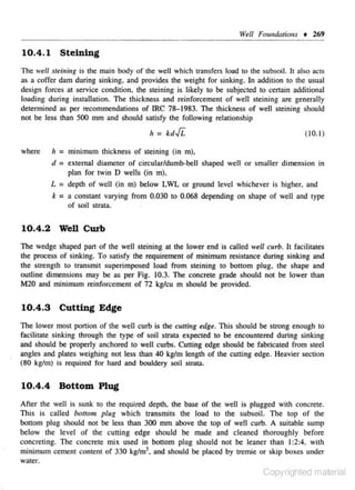
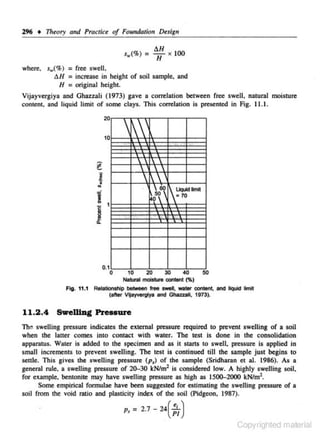
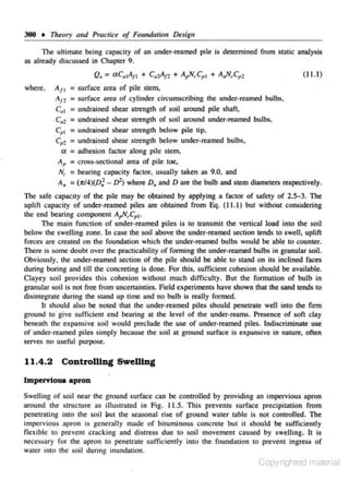
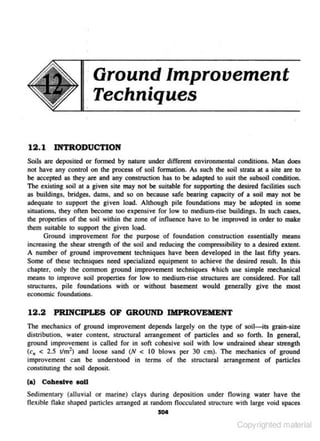
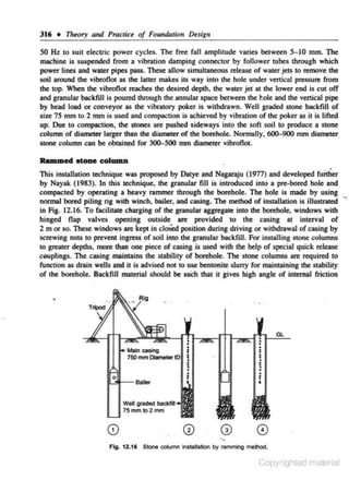
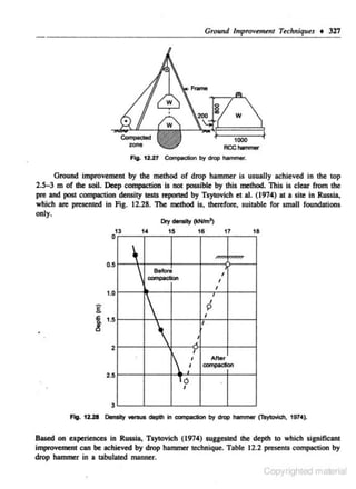
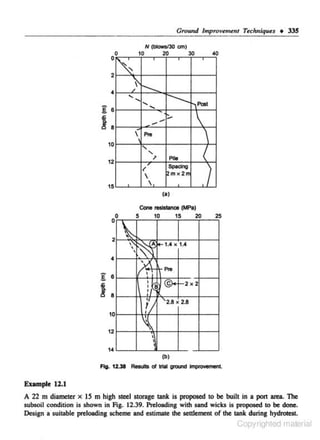
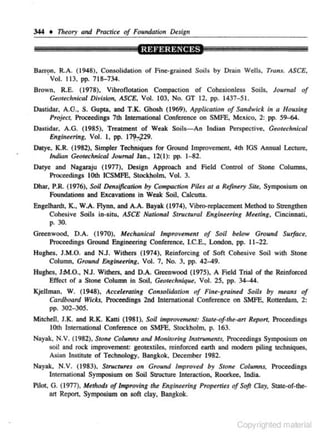
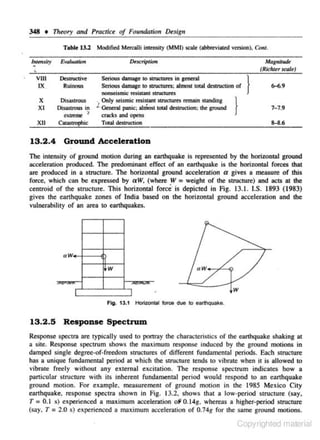
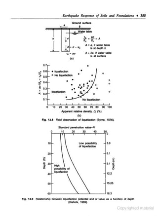
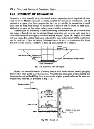
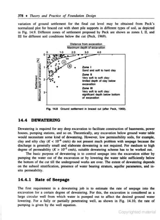
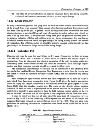
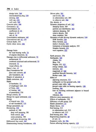
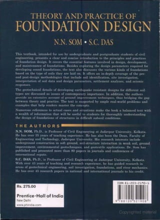
49. 1. 10 SOJL DEPOSITS OF INDIA
Tile soil deposita of lncha m:~y be classified under most of lhe ~minant aeological
formations (dcscnbed earlier). namely
(b) Marine depositS
(c) Dcsen ooll
(a) Alluvial oolls
(d) Laterite soil
(c) Sleek cotton ooll
(f) Boulder depositS
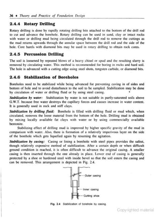
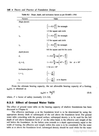
Figure 1.26 shows the di01ribution of predominant soil deposits in India (Ranjan and Rao
2000).
32°
2$.
z•·
2&·
23.$.
zo•
~AA.MIIt
18"
.-a•ll
mo.-.-
m---
tr
r;m~on~~-
12"
IZ3-~
& ' ! ] - dopoOIII
54·
aa·
1'2"
16·
eo-
54·
aa·
92"
ga·
1ocr
Fig. 1.26 Soil deposits of lndta.
Allu..W aoUa
Large parts o( northern and CIStern India lyina; in the lndo-ao.naetic plains and the
Brahmaputra valley arc covered by the sedimentary deposits of the river> and their
tributaries. Tiley often hove thickness greater than 100 m above lhe bed rock. Tile deposits
..-ly constitute layer> of sand. sdt. and clay depending on lhe pDOJtion of lhe river away
from lhe soun:c.
llarlDe depoe.IU
India has a long coast line extending along lhe Arabian sea. Indian ocean, ond lhe Bay of
Bengal. n.e deposits along the coast are mostly laid down by lhe sea. 11leiC marine c lays of
India are generally soft and often contain organic matter. 'They pOCSC$$ low shear strength
and high compresSibility.
<..opynghted matenal

50. 30 • Theory and Practice of Fomtdation Design
Black cottOD ooU
The central p:lrt of India has extensive deposits of the exp:msive soil known as black couon
soil. This covers wide areas of Maharas tra, Madhya Pradesh, Karnataka, Andhra Pradesh,
Tamil Nadu. and U11ar Pradesh. The soil contains montrnOrillonile clay mineral which has
high swelling potential.
Laterite IOU
This soil covers wide areas of Kerala. Karnati.lka. Maharasua, Orissa. and pans of West
Bengal. Lalerites are residual soils fonned by decomposition of rock which fonns oxides of
iron and aluminium.
Desert IOU
Large areas of Rajasthan in lhe Thar desert are composed of wind blown deposits of desert
soil. like loess. The sand dunes are often 15 m high and are formed under highly arid
conditions.
Boulder depoetto
Boulders are deposited is hilly rerrains where the rivers flow wilh high velociry and carry
large size boulders. These deposits are found in the sub-Himalayan regions of Uttar Pradesh
and Himachal Pradesh.
Barkan. 0.0 (1962), Dynamics of Bases and Foundations, McGraw Hill Book Co., New
York.
Bishop. A.W . (1959), The Principle of Effective Stress, Teknisk Ukebald, Vol. 106, No. 39,
pp. 859-863.
Bishop, A.W. ( 1966), Strength of Soils
pp. 89-130.
as Engineering Materials, Geoteclrnique, Vol. 16,
.
Bishop, A.W. and OJ. Henkel ( 1964), The Meilsuremeni of Soil Prop<rtus in the Triaxial
Tw, Edward Arnold, London.
Bjerrum. L. (1964). R~lasjon M~lom Malte og Berengnede Serninger av Byggverk pa Leire
og Sa11d, Norwegion Geotechnical Institute, Oslo, Norway.
BoWZ<~k
ond G.A. Leonards (1972), The G/oucnt<r Test Fill. Proeee&ngs ASCE Speciality
Conference on performance of earth and eanh retaining Sln.lctures, Lafayette. Indiana.
USA.
Burlond, L., F.G. Buller. and P. Ouniean ( 1966), The Behaviour and Design of lArge
Diometu Bored Piles in Stiff Clay, Proceedings SympOsium on Large Bored Piles. The
lnslilUtion of Civil Engineers. London, pp. 51- 71.
Copyrighted material

51. Soil as arr fngineerirrg Material • 3 1
Chummar, A.V. (1976), Foundation Problems b1 Cochln, Proceedings Symposium in
Foundations and Excavations in Weak Soil, Calcuua, Vol. I, Paper No. C 4 .
IS 1498 (1970). Classification and Identification of Soils. Bureau of lodian SWldards, New
Delhi.
Lambe, T.W. (1962), Por<-pr<ssur<s ilr a Foundation Clay 1962, Proceedings ASCE. Soil
Mechanics and Foundation Division, Vol. 88, pp. 19-47.
Marsland. A. ( 197 I). The Shear Strengths of Stiff Fissur.d Clays, Proceedings Roscoe
Memorial Symposium, Cambridge, U.K., pp. 59~8.
Menard, L. (1956), An Apparatus for Measuring tire Strength of Soils in P/Qce, MS. Thesis,
University of lllinois. Urbana, lllinois, USA.
Ranjan. G. and A.S.R. Rao (2000), Basic and Applied Soil Mechanics, 2nd edition, New
Age International (P) Ltd.. New Delhi.
Schmertmann, J.H. (1953). Undisturbed Consolidation Behaviour of ClayJ. Transactions.
ASCE, Vol. 120, p. 1201.
Scott, R.F. (1965), Principles of Soil Mechanics. Addison Wesley. Boston, USA.
Skempton, A.W. (1948), The ~ = 0 At~alysis of Stability and its Theoretical Basis,
Proceedings 2nd International Conference on SMFE, Vol. 2.
Skempton, A.W. and A.W. Bishop ( 1954), Soils, their Elasticity and Inelasticity. North
Holland Publishing Co. Amsterdam.
Skempton, A.W. and R.D. Northey (1952), 17re Sensitivity of Clays, Geotechnique. Vol 3,
pp. 30-54.
Taylor, D.W. ( 1948), Fundamentals of Soil Mechanics, John Wiley & Sons, New York.
Terzaghi, K. and R.B. Peck (1967). Soil Mechanics in Ei1ginuring Practiu, 2nd edition,
John Wiley aod Sons, Inc. N.Y.
U.S. Depanment of Navy (1971), Design Manual-$oil Mechanics, Foundations and Earth
Structures, NAVFAC. DM- 7. U.S. Government Printing Office. Washington, D.C.
Copyrighted material

52. II
II
Site In estigation
2 .1 INTRODUCTION
ll is essential to carry OUt site investigation
preparing the design of civil engineering
works. The investigation may range in
from simple examination of the surface soils.
with or without a few shallow lrial pits.
a detailed s1udy of the soil and ground water
conditions for a considerable depth below
ground ·surface by means of boreholes and in·
situ and/or laboratory tests on lhe soils :~~~~~!. 1be extent of the investigation depends
on the imponance of the stNCture. the c•
of the soil conditions. and the infonnation
already available on the behaviour of
foundations on similar soils. Thus, it is not the
normal practice to sink boreholes and
soil leSLS for single or two-storey dwelling
houses since normally. there is adoquale
of the safe bearing pressure of the soil in
any particular locality. Only in
soils such as peat or loose fill would it be
necessary to sink deep boreholes.
supplemented · by soil tests. More extensive
investigation for light st~tures is needed
structures are buih on filled·up soil or in
ground conditions where there is no
available on foundation behaviour of similar
structures. A detailed s ite investigation
deep boreholes and laboratory testing of
soils is always a necessity for heavy
such as bridges~ multi-storeyed buildings or
industrial plants.
Thus. the major objectives of site inveftigatuon are:
1
(a) Knowing the general suitability of
site for proposed works.
(b) Assessing local conditions and proj>lems likely to be encountered in foundation
construction.
(c) Acquiring data for adoqua1e and ecxf>otmic design of foundlltion.
2 .2
INFORMATION EJJ::TB:A.C:TJI;.> FROM SITE INVESTIGATION
A lot of information is extracted from site iqv·estigattion to facilitate foundation design. This
includes
I. General topography of the site whii h affects foundatio n design and construction,
presence of water courses. and so on.
e .g .. s urface c.o nfiguration, adjacent
Copyrighted material

53. Sile lnvesn'gation
t
33
2. Location of buried services such as power lines, telephone cables, water mains,
sewers pipes and so on.
3. General geology of the area with particular reference to the principal geological
formations underlying the site.
4. Previous history and use of the site including information of any defects and failures
of struc.turcs built on the site.
5. Any special features such as possibility of earthquake, flooding, seasonal swelling etc.
6. Availability and quality of local construction materials.
7. A detailed record of soil or rock strata, ground· water conditions within the zone
affected by foundation loading and of any deeper strata affecting the site conditions
in any way.
8. Design data which comprises strength and compressibility characteristics of the
different strata.
9. Results of chemical analysis on soil or ground water to detennine pos.'ible deleterious
effects on foundation structures.
2 .S
STAGES OF SITE INVESTIGATION
Different stages of site investigation for a major civil engineering project may be summarised
as shown in Table 2.1.
T able 2.1 Stages or site investigation
ReconMissance Study
(I)
Geological -
(b) Ptdologlcal data
(c) An:al photographs
(d) Geophysical investigaaion
Dt-roild JnwstigatWtt
(I) Boring
(b) Sampling
(C) Ttstioa
(i) Lab test
(ij) l"!dd ""'
(d) Aerial phococnphs
(e) Geophysical melhods
P~tjOnrt(JM,
Study
(I)
further testing
lnsuwn<nwion
(c) Paformance evaluation
(b)
2 .S . l
ReeonnaisaaDee Study
Roconnajssancc study involves the preliminary feasibility study that is undertaken before any
detailed planning is done-mainly for the purpose of selection of site. This is to be done at
minimum cost and no large scale exploratory work is usually undertllken at this stage. The
required data may be obtained from:
Copyrighted material

54. 34
t
TI1eory and Practice of Fou11dation Design
Geolo~cal
ourny reporto and mape
Geological interpctation of land forms and underlying strata give !he .sequence of events
leading to the formation of subsoil deposits. They help to define the propenies of the
material in a general way.
·
Pedolo~cal
dot&
Many areas have been surveyed for agricultural purposes-usually to depths of 2 or 3 m.
Materials arc often classified according to colour, texture, chemical composition, and so on.
Aerial photocrapha/aateWte lmageo
Photographic representation of a portion of earth· s surface taken from the air or space.
Geophya.lcal methodo
Applica6on of the methods and principles of physics to detennine the propenies of
s ubsurface materials. These methods are particularly useful for identifying bed rock. Seismic
refraction method or electrical resistivity tests are usually done for this purpose.
2.4 BORING (DETAILED SOIL INVESTIGATION)
Detailed soil investigation is done through a series of boring, sampling, and testing to obtain
the en.gineering properties of soil. The following subsections are devoted 10 boring which
discuss different methods of boring in detail.
2.4.1
~al
Pit•
Trial phs arc the cheapest way of site eltploration and do not require any specialized
equipmenl. A pic is manually excavated to get an indication of the soiJ stratification and
obtain undisturbed and disturbed samples. TriaJ pits allow visuaJ inspection of any .change of
strata and facilitate in-situ tesling. They are. however, suitable for exploration of shallow
d4:plh only. Figure 2.1 is a diagrammatic representation of trial pitS.
Test pit
Brownish grey
silly (jay
Soil Strata
F1Q. 2.1
2.4.2 Wash
Trial pit
BoriDC
A hole, usually 150-200 mm diameter, is advanced into the soil through a suitable cutter at
the bonom of a drill rod. The soil is loosened and removed from the borebole by a stream of
water or drilling mud, issuing from the lower end of the wash pipe which is worked up and
Copyrighted m3erial

55. Sitt' Juvestigtaion • 35
down or romted by hJind in the borehole. Water or mud now carries the soil up the onnular
space between the wosh pipe ond the cosing. ond it overflows ot ground level where the soil
in suspension is allowed to settle in a tank and the fluid is re·circulated or discharged to
waste as required. Samples of the settled soil can be retained for identification purpOses.
Figure 2.2 shows the arrangement for wash boring.
Waktr
Winch._
awiveJ
Pump
Engine
Sump
Wash pipe
'
Flg. 2.2 Wash boring,
The method is simple and cheap. The structure of the soil below the boring apparatus is not
disturbed and thus, both disturbed and undisrurt>ed samples can be obtained.
2.4.3 Auger Boring
In this method. the borehole is advanced by turning a.n auger into the soil, withdrawing it
and removing the soil for examination and tes1. The auger is re· inserted for further boring.
The auger may be manually or mec.hanically operated. Extensions are added to reach
the desired depth. Disrurt>ed samples may be obtained from the soil brought up by the auger
while undisturbed samples nrc obtained by pushing sampling tubes at suimble intervals in the
borehole. The apparatus for auger boring is shown in Fig. 2.3.
~Handle
1- Dril
-
-~
....
I
I
I
I
I
I
Post.flole auger-
'
rod
t
I
I
I
I
''
:
•
I
Fig. 2.3 Auger bof'lng,
Copyrighted material

56. 36 • Tlreory and Practice of Fowu/n1ion Design
2 .4 .4
Rotary Drllling
Rotnry drilling is done by rapidly rotating drilling bits attached to the bottom of the drill rod
to cut and advnnce chc borehole. Rmary drilling can be used in sand, clay or inl,act rocks
wilh warer or drilling mud being circulnted through che drill rod to remove the cuttings as
the mud returns u pwards chrough che annular space between the drill rod and the side of the
hole. Core bnrcls wilh diamond bits may be used in r01ory drilling co obtain rock cores.
2 .4.5 Percussion Drilling
llle soil is loosened by repeated blows of a heavy c hisel or spud and the resulting slurry is
removed by c-rculating wacer. This rnelhod is recommended for boring in rocks and hard soil.
i
The hole is advanced with o cuuing edge using sceel shots. lung:scen carbide. or djamond bits.
2.4.6 Stabi.Uzatlon of Boreholes
Boreholes need 10 be stabilized while being odvanced for prevenring caving in of sides :md
bottom or hole and to avoid disturbance to the soil to be sampled. Stabiliuuion may be done
by c irculation of woter or drilling flu id or by using steel casing.
"
Stabilit.ation bJ water: Stabiliz.ation by water is not suitable in partly-saturated soils above
G. W.T. because free water destroys the capillary forces and causes increase in w:.ter content.
It is genemlly used in rock and stiff clays.
Stabilization by drilling fluid:
Borehole is fi lled with drilling fl uid or mud which, when
circulated. removes the loose material from the bottom of the hole. Drilling mud is obtained
by mixing locally available fat clays wilh water or by using commercially available
bentonite.
Stabiliz.ing effect of drilling mud is improved by higher spe-cific gravity of the mud in
c,omparison with water. Also. there is fonnation of a relatively impc.rivous layer on the side·
or che borehole which getS liquefied again by resuming the agitation.
SlabiliUJilon by ca.ti11g: Casing or lining a borehole with steel pipes provides the safest.
though relalively expensive method of stabilization. After a ce11ain depth or when difficult
ground condition is reached, it is often d ifficult to adv::mce the original cas-ing. A smaller
casing is 1hen inserted through the one nlready in place. Lower end of casing is generally
protected by a shoe or hardened steel w-ith inside bevel so that the soil enrers the casing :md
c.on be removed. This nrrangel'nenl is depicted in Fig. 2.4.
:::r-
t--Outer casing
r-
f- f't- Inner casing
ll-+Fig, 2.4
Cutting shoe
Stabilizaclon or t>orehose
by castng.
Copyrighted material

57. Sit~ l11~srigation
+ 37
Exccpr when undisrurbed samples ore required in ~nsitive clays. !he casing is genernlly
driven by repeUicd blows of a drop hammer. Casing prevcnrs side caving, bur nor always
bottom caving. This can be achieved by filling the casing with water or driiJjng fluid.
However. casing should nor be filled wirh warer if bonom of casing is above ground warer
table and undisturbed samples are required.
2.5
SAMPLING
The different types of sample obtained from boreholes are shown in Table 2.2.
Table l..l Types of sample
SampJ~s
Undisrurbed
OiSIWI>cd
I
RtmdUidcd
R~ve
(The structure of the soil is disturbed
to a consjderable degrte by che action
of boring toots and ucavation equipment.)
2 .5.1
(Retains as closely as practicable.
lhe true in-shu structure and
water cornen1 of the soiJ.)
SampUng from Trial Pits
Block samples (refer Fig. 2.5) are hand cur from trial piiS or open cxcavarions. A block of
clay is c--arefully trimmed with a sharp knife. taking care that no water comes into contact
wilh rhe sample. Good quolity samples can be obtained by this merhod. but if the soil does
nor possess ony cohesion. ir may be dirticuh, if 001 impossible. 10 obi:Un block samples.
Fig. 2.5
2.5.2
Bloc:k sanplc.-of clay,
SampUng from Boreholes
Undisturbed samples may be obtained from boreholes by open drive samplers or piston
samplers. An open drive sampler is shown in Fig. 2.6.
Drift
rod
Fig. 2.6 Open drive sampler.
Copyrighted material

58. 38 • Theory alld Practice of Foundation Design
Open drive samplers consist of thin-walled tubes which are pushed or driven into the
soil at the bottom of the hole and then rotated to detach the lower end of the sample from
the soil as shown in Fig. 2 .6. Most soft or moderately stiff cohesive soil can be sampled
without extensive disturbance in thin·walled seamless steel tubes having diameter not less
than 50 mm. The lower end of the tube is sharpened to from a cutting edge and the other
end is machined for attachment to drill rods. The entire tube is pushed or driven into the soil
at the bonom of the hole and is removed with the sample inside. The two ends of the tube
are then sealed and the sample shipped to the laborntory.
Good quality undisturbed samples are obtained from piston samplers which use thinwalled sampling tubes with a piston inside. While the tube is being lowell:d to the bouom of
the drill hole, the piston rods and the piston are held at the boltom of the sampler by means
of a drill rod which rises to the top of the borehole. A pislOn sampler ls shown in Fig. 2.7.
The presence of the piston prevents excess soil from sequeezing into the tube and thus.
maintains the integrity of the sample.
-Fi9- 2.7 f'lsiDn sampler.
Table 2.3 lists the requirements of a good sampling tube (ll:fer Fig. 2.8) as follows:
Flog. 2.8 Sampling tube.
Copyrighted material

59. Site brvesagotiou • 39
T able 2.3
(a) Area ralio, C =
.
Requiremenls of sampling tube
1
1
o.. - oc
o'
•
This represents the amount of soil that is displattd when the sampler is forttd into lhc: ground. Thicker the
tube. more is tht diswrbanet". The ateil ratio of a good sampling tube should not cxct:cd ISIJt.
(b)
Inside clearance ratio, C1 = D, ~ D,
For
•
lonJ sampl... 0.75% < C, < I.S%
o.scx,
For shon samples. 0 < C1 <
The diameter of the sampling tube is kept slightly larger than the diameter of the cuuing edge to minimise:
friction on the sampJe as it enters the: sampling tubt.
(c) Outside clearance ratio,
c. =
D,.;, D,
• :Z..J'h
'Tbis dearance is provided to mluce &he drivlog fOl"Cle requlttd to penetrate the sampler into the soil.
DiametO" of samples should 001 be less !han 38 mm. In gcn<nl. SO. ISO mm diamelel' undUwrb<d samples
are obtained from boreholes.
2.15.3 Preaervatlon of Samples
Undisturbed samples which ""' to he tested after some time should he maintained in such a
way that the natural water content is reraincd and no evaporation is allowed.
Usually. two Co ats of 12 mm thick paraffin wax. and pelrolcum jelly are applied in
·
mohen state on either end of the sample to keep the water content unchanged for
considerable time when the sample is preserved in o humidity controlled room. In the
absence of such fa<:ili ties, the sampling tubes should he covered by hessian bags and sprinkled
with water from time to time. Block samples may he coated with 6 mm thick paraffin wax
and kept in air·tight box w:·h saw dust filli ng the annular space between the box and the
sample. Figure 2.9 shows sol..e typical arrangements for preservation of samples.
Cover
Paraffin coat
~b'a<allin coat
(Paraffin wax +
P&ttOiel.wnjelly)
$ample Wooden box
(a) Block sample
Saw dust
(b) Tube sompte
Fig. 2.9 Preservation of sam ples.
Copyrighted material_

60. 40 + Theory a11d Practice of Foundation Design
2.6 TESTING OF SOIL
Soil properties arc determined from appropriate laboratory and field restS. The specifications
regarding laboratory tests and field tests for routine soil investigation are given in
Tables 2.4 and 2.5.
Tabl~
l .4
Laboratory cesting of soils
T~ o/lt!St
ProJHTt'JI of soil
Qualiry of samplt
C/4ssifo:4tlon
I.
2.
3.
l~ fication
VisuaJ soil classification
RID
Grain size distribution
(a) Sieve analysis }
(b) Wet analysis
D
Consistency limits of
(a) Li<jwd limit
(b) Plastic U
mit
cohesive soils
}
RID
(c) Shrink~t~e limit
4.
S.
Moisture content
Unit weight
UKit~tuing
I.
Moisture contctlt
Spcdfic gravity
UD
0
propntin
Shear stren&th
(a) Unconfined compression }
(b) Din:ct .!lew
2.
3.
4.
Cornpr=ibility
UD
(C) Triwal (UU/CU/CD)
(a) Ocdomelerl<$1 1
UD
(b) Tri>.xial ....
(a) Constant head pcrmeabUil)'
(b) Varioble head permeability test
1<$1)
l'<rnle>bility
(a) Proctor cesc )
Compaction characteristics
{b) CBR teSI
5.
Chemical and mlnetaloglcal
composition
(a) X-Ray diffracnon
(b) D.T.A.
UD
I
RID
RID
(<) 01emical test
R-Reprts<:Dtative
D-Dishubcd
T able 2.5
UD-Undistu.rbed
Field testin.a of soils
TyfH of tat
I. Relative densiry (granular soils)
2. Shear strength (cohes:ive soil)
(a) Standard penetration lt$l
(b) Dynamic cone cest
(a) Vane test
(b) Direct shear test
(c) Sialic cone
3.
4.
Bnring capacity and seu.Jement
Permeabilily
ln·situ strength and deformation
Plo<e bearing teSI
(a) Borehole/pumping tes1
(b) Pierometer teSI
load cest
(a) Moisture-density rel;nion
(b) In-pioce density
(c) C.B.R. test
(a) Prts.suremeL test
cr
ch!ln•cteriscics
(b) Dilotomctcr tt:sl
S. Testing of piles
6. Compaction conU'OI
7.
test
or soil
Copyrighted material

61. Siu lnvestigalion • 41
2 . 7 FJEI.D TESTS
2 .7 .1 StiiDdard Penetration Test (SPT)
It is extremely difficult to obtain undisturbed samples of granular soils, so in-situ SPT is
performed at frequent intervals along the depth of a borehole. A slllndard split spoon sampler
(Fig. 2.10) is driven 45 em into the gnnund by means of a 6S kg hammer falling freely from
a height of 75 em. The toW number of blows required to drive the second and third depth
of IS em (i.e. total 30 em) is called the slllndard penetration resistance (N blows per
30 em). After the blow counts are recorded. the spoon is withdrawn and a representative
sample is obtained for identification tests.
To dril rod
t
SIOOI somplng
. _ 2"(5(1).8)
(split klngiludinally)
Fig. 2.10 SPT -
·
For cohesive soils. a simple correlation between the slllndard penetration resistance (N)
and the undrained shear strength, c, has been proposed by Stroud (1974),
c, = kN
(2.0)
when: k is a constant having an average value of 4.5 kN/m2. Similar relationship has been
obtained by SengupUI (1984) who studied the correlation for some cohesive soils and
obUlined a value of 4.2 for the consUlnt k. Terugbi and Peek's relationship has been widely
used to obtain the consistency of cohesive soils in terms of the undrained shear strength, as
shown in Table 1.9 (Terzaghi and Peck, 1967).
In granular soils, the SPT blow count is affected by the effective overburden pressure,
u.;. So. N value obtained from the field should be corrected to correspond to a standard
vaJue of
a...'. Accordingly,
(2.1)
Copyrighted material

62. 42 • T1reory and Practice of Foundation Design
where
Ncvt = corrected N value for a standard value of a.,' (1 00 kN/m2)
C,. = correction factor
Nr = N value obtained from field
The correction factor C,. may be taken from the empirical relationship given by Skempcon
( 1986).
2
(2.2)
C, = I + O.Olcf,
where a,' = vertical overburden pressure in kNim2
A dilatancy correction has been recommended for saturated fine sands and silts to
account for the development of negative pore pressure. if any, during driving of the SPT
sampler and consequent increase of shear strength and higher SPT blow count (Terz.aghi and
Peck, 1967). For such soils that have N"" greater than 15 as per Eq. (2.1), a conection for
dilatancy may be made as,
N
= 15 + 0.5(N.., - 15)
(2.2a)
The relative density and the degree of compaction of granular soil can be obtained from
Tenaghi's empirical correlation, as in Table 2.6.
Table l..6 Relative density from SPT blow oount
No. of blows
R'latiw tki&Sity
(N/30 em)
R0 = ( • • ., - ' ) x 1001&
'-... - ~"min
C)-4
Q-15~
4-10
tQ-30
IS-35%
25-651&
6S-85'.6
> 85
3o-SO
>so
Very 10050
Loose
Mcdlum
Dense
Very Dense
Many attempts have been made to obtain empirical correlation between NC!OI and the angle of
shearing resistance of sand. The most recent attempt by Halanakar and Uchida (1996) appears
to agree well with laboratory test data, which gives
,z,j20N~ + 17 degrees
(2.3)
The modulus of elasticity is obtained by the relationship given by Mezenbach (1961) as
E = C1 + C:/{ kg/em'
(2.4)
where C 1 and C2 are functions typical of the type of sand. Some C 1 and C 2 values
corresponding to different soil types are given in Table 2.7.
Copyrighted material

63. Sitt lm·estigotUm • 43
Table 2.7
Modulus or elasticity or sand
C, (kstcm'l
Soil t}JH
C1 (tgtcm1/blow)
52
3.3
4.9
Fine sand (above G .W .T)
Fine sand (below O .W.T)
3. Sand (Medium)
4. Coarst sand
5. Sand + cravel
6. Silty sand
7. Sih
I.
2.
71
39
38
43
4.5
lOS
11.8
24
5.3
12
5.8
A similar correlation between the compression modulus E and the SPT blow count N
has been obtained by Papadopoulos (1992). This is given by
E = 75 + 8N (kglcm2)
(2.4a)
Bowles (1988) also gives useful relations to evaluate the srress~strain modulus of sand
from SPT blow count, as shown in Table 2.8. But they generally give very conservative
values.
Table 2.8 Stress-strain tNXlulus of sand (Bowles. 1988)
TyfH' of sond
Sand (noonally oonsolidated)
Sand (""'r31ed}
Sand (ove"""solicbted)
Sa.nd with gravel
Silty sand
E (kglem2)
S(N + IS)
2.S(N + IS)
7.S(N + 24)
12(N + 6) for N > IS
&_N + 6), N S IS
3(N + 6)
Although standard penetration test is basically a qualitative test, correct interpretation of
data gives good evaluation of soil properties particularly in granular soil. The main sources
of error include inadequate cleaning of borehole. eccentric hammer blow, and presence of
large boulders and gravels which give erratic results.
2 .7 .2 Dynamic Cone Penetration Test (DCPT)
Dynamic cone penetration test is done by driving a standard 60° cone attached to a drill rod
into the soil by blows of 65 kg hammer falling from a height of 750 mm. The blow count
for every 30 e m penetration is made to get a continuous record of the variation of soil
consistency with depth. The test does not need a bo"'hole. It can be done quici<Jy 10 cover a
large area economically. The test helps to identify variability of subsoil profile and to locate
soft pockets, such as filled up ponds. When DCPT is carried out c lose to a few bo<eholes,
suitable correlations may be obtained for a particular s ite and the number of boreholes can be
reduced.
The dynamic cone penerrotion test is done either by using a 50 em diameter cone or a
65 mm diameter cone with circulation of bentonite slurry to eliminate friction on the drill rod.
One of 1he proposed correlations between Ned obtained from DC.PT and Nt« obtained from
SPT is
Copyrighted material

64. 44 • Theory a11d PractU:e of Founda1ion Design
N,. = (1.5 - 2 )N""
(2.5)
These correlations can be used to obtain the SP'f blow count, N from DCP'f data.
2.7.3
Static Cone Penetration Test (SCPT)
The static cone penetration test (SCPT) is a direct sounding test which is done to obtain a
continuous record of soil characteristics with depth and to estimate their e ngineering
properties. The test does not need any borehole. A 60" cone having an apex angle of 60" and
a base area of 10 cm1 with a friction jacket above. is pushed into the ground at a steady rate
of 20 mmfs. Modem static cone penetrometers have e lectrical measuring devices with wires
from the transducers attached to the cone and the friction jacket giving continuous record of
the cone and friction resistances as illustrated in Fig. 2,1 J.
1
8
6
4
3
3
2
1
Fig. 2.11 Strie cone penettomeetr (tltettic:al). 1. Conical point (10 crn2): 2. lOid ctll; 3. Strain gauges;
4. Friction sleoYO {!50 an'); 5. Adjuslment ring; 6. Walerpf<>Of bushing;
7. Cable; 8. connection with rods
The test measures the cone resistance. q~. developed against the penetration of the cone and
the frictional resistance, /, developed between the sleeve and the surrounding soil as in
Fig. 2.12.
,,~hn'l o, kNJm'
2.5
0
;
:
,)
·' 5
t
1000
2000
S_ ..,_
_...
~
-
..
~
._
1
"' 'l::..
b:·-'~
-~y
.-••...
'
$
20
•
1:
~
~
;;;;;.:
'
,s
25
!
Fig. 2.12 Static oone penetrometer data.
Copyrighted material

65. Site Investigation • 45
Typical penetrometer test data give a continuous variation of the cone resistance and the
frictional resistance with depth. In recent years. the static cone penetrometer has been
modified to incorporate an electrical piezo-cone to give simultaneous measurement of tip
resistance. side friction and the pore pressure as the cone is advanced in lhe soiL The
development of pore pressure makes the interpretation of soil type more accurate in terms of
permeability of che soil.
Lancellotta (1983) and Jamilkowski et al. ( 1985) proposed an empirical correlation
belween the relative dens-ity of nonnally consolidated sand. D, and q,..
D..(%)
= - 98 + 66 1og10
(}?)
(2.6)
where a' := verticaJ effective stress at depth considered and both qt' and a' are in units of
tonnes per sq. m.
This relationship is based on che oorrelation obtained from several sands as depicted in
Fig. 2.13.
95
85
D, = -98+
IW!tog,o((q~~·)
75
a; In ten (meltlcYm'
• Ticino aand
• 0t1awa sancs
q, and
45
• Edgar sand
• Hol<l<Mindsand
• Hilton mine Sind
Flo. 2..13
Relationship bet-Neen c:one penetration resistance and relattve density
(alief Jamiii<OWSIII ot al., 1985).
The peak friction angle •• of normally consolidated sand may be obtained from the
expression. (Kulhawy and Mayne 1990),
;- = tan-•(o.l ...
o.381og~)
(2.7)
For cohesive soil, Mayne and Kemper (1988) gave the following relations for the
undrained shear strength c,., preconsolidatjon pressure Pr• o.nd the overconsolidation ratio.
OCR as
Copyrighled material

66. 46 • Theory aud Practice of Foulldation Design
.... q, - a.,
c. -
20
16
p, = 0.243 (q,)"-'
(2.8)
OCR = 0.37 ( q, ~. " • )
1.0 1
where a" and a:. are the total and e ffective vertical stresses at the level of test respectively.
Some useful relalionship be1ween q, and !he SPT blow counl have also been oblained
by Robertson and Campanella (1983). The range of variation of q,JN, wilh mean grain size
D, is illus1
ra1ed in Fig. 2. 14.
Clay
Clayey slit & Sandy silt
sfJty d ay
and silt
Silly sancl
1000
//
900
/
800
/
//
700
v,.....
Range of results of Robertson &
C..mpanella (1963)..,
300
200
100
0
v
,....."
-- ,..--- ---
___ ....
<
.).. _..;>..;:
~-.::
:---
~--- -
lnela
..... .....
,.....'
~/
~
Average of Robertson &
.
.
0,01
0.001
/
/
0. 1
Mean grain size.
(1963)
• 1.0
D,o (mm )
Flg. 2.14 Rangt Of vatlation Of Q1
/N~
Meyemof's (1965) simple correlation between q, and N for fine 10 medium dense sand is also
eX!eliSively used. This relation is expressed as
q, = 4N
where qr is in
(2.9)
kg/cm 2•
2.7.4 Vane Shear Test
Vane shc"r test in cohesive soils obvintes the difficulty of obtaining un~disturbed samples and
arc particularly suitable for sensitive clays. This test facilitates "averaging·· the ma.u
chnracteristics or soil in-situ.
Copyrighted material

67. Site ltrvestigotio" • 47
A four bladed vane ac the bouom of a drill rod is pushed into the soil and a torque is
applied by turning a handle at lhe top to create a cylindrical shear surface. as depicted in
Fig. 2.15.
p
go•
1<---s--+1
go•
Torque head
p
Torque
rod
Vanes
-Pvanes
~<'-0->0
Fig. 2.15 Vane shear test arrangement
At failure. the shear strength of the soil is related to the applied torque by the relationship
2
T
= 1<D H
2
(I +.!_ D )~
3H
(2.1 0)
where,
D ::diameter of sheared cylinder
H
~
diameter of vane
=Height of vane
T = Shear strength acting along the surface as weU as at the top and bottom of the
sheared cy Iinder.
The assumption that the shear stress is uniformly distributed across the top and bottom
is questionable but the variation due to any other assumed distribotion is not great. Normally.
SO mm diameter x 100 mm Jong four bladed vane is used and the vane is rotated at the rate
or 0.1 degree/s. Both undisturbed and remoulded strengths can be determined by first finding
the undisturbed strength and lhen rotating the vane fully to obtain lhe remoulded strength.
2.7.5 Direct Shear Test (In-Situ)
In-situ direct shear test, depicted through Fig. 2.! 6. is particularly suitable where tests on
small specimens are not representative or lhe performance or the in-situ soil. e.g. fissured
c lays. The test has been done extensively on London clay (Bishop 1966).
Copyrighted material

68. Tlt~ory
48 •
and Practice of FoUirdation Design
Peak
strength
-~~~
strength
J...----tr Hydraulic
jadt
Test
1
1'S
Shear displacement
jack
Ftg. 2.1&
lr»>tu dWed. shear tHl
2. 7 .6 Plate Bearing Test
To study the bearing capacity and settlement behaviour of soils, a suitable method is to test
a full scale foundation under its design load long enough to observe all set~ement. However,
this is rarely possible because of the time required for full consolidation and the heavy load
required to produce a bearing capacity failure. As a substitute, small scale plate load tests are
performed. The load can be applic;d by dead weight or by jacking against a reaction.
The test is caJTied out in a pit with either circular or square plateS of width/diameter
300-750 mm. The size of the plate should be as large as possible and consistent with the
capacity of the loading device. The load is increased in increments of about !/lOth of the
estimated failure load or 1/Sth of the proposed design load until complete bearing capacity
failure or twice the design load is reached. A plot of settlement versus load intensity is then
Obtained as in Fig. 2.17.
Pressure
1M:
I
I ~------
:CN!t
I
I
Fig. 2.17 Plale toad test data.
The failure load is given by the intersection of initial and final tangent. If no well
defined failure point is reached, the data are plotted on logo versus logp scale to obtain the
point of intersection. failure may also be taken to be the point corresponding to an
arbitm.rily chosen limit of settlement., depending on the requirement of the suucrure.
Knowing the failure load and deformation char.acteristics from plate load te,st. the shear
strength and modulus of elasticity of the soil may be obtained from corTelation with be:lring
capacity and settlement equations of shallow foundations.
Copyrighted material

69. Sitt
lnv~stigalion
• 49
UmJtatloaa of lOild teata
The limitations of plate load test arise out of
(i) Extrapolation on the basis of theory of elasticily and/or empirical relation is only
approximate due to non-homogeneity of the soil. Some agencies recommend the use
of plates of different sizes and extnlpolation for the actual foundation.
(ii) Load test data reflect the ch311lCteristics of a soil only within a depth aJ>I.roXimately
equal to twice the width of the plate.
(iii) Plate loading test is essentially a short term test (run in a few hours), so no
indication of the long tenn consolidation behaviour is oblained.
(iv) The load toot data alone do not give full indication of the properties of a subsoil.
Bu~ used judiciously in conjunction with other test data, it has valuable use in
design, particularly in estimating the settlement of cobeslonless soil.
2 .7 .7
Preuuremeter Test
Menard (1956) developed the pressuremeter test to measure the strength and deformation
characteristics of soil in-situ. The test is done at different depths in a borehole with the help
of a pressuremeter which consists of an expandable probe with a measuring cell at the centre
and two guard cells at top and bottom. One such lfl1lRgement is shown in Fig. 2.18.
-
Cowlter Ll'lit
gas IUPil'Y
Tubing (gas
and ---l-o-/
wablt lines)
Fig. 2.11 Menotd pressuremelef.
The probe is inserted in a pre-boned hole and is expanded in volume either by liquid or
air pressure until the soil fails or the expanded volume of the measuring cell reaches twice
lhe original volume of the cavity. The guard cells are used to minimise the end effect on the
measuring cell. Table 2.9 gives the typical dimensions of the probe and borehole.
Copyrighted material

70. SO • TI1eory and Practice of Foundation Desig11
T1blt 1.9 Dimensions of prusuremeter probe and borehole
H
ole
Dlamtrtr of
1..
L
tksignation
pro!>< (nun)
(m)
(m)
Ax
44
36
Bx
Nx
S8
21
66
42
70
2S
Bortholt dia (mm)
Nominal Ma.timr1m
46
52
60
66
so
72
48
Figure 2.19 shows typical resulcs of a pressuremecer test. The expanded volume of the
meaSllring probe is plotced against the applied pressure. The curve is divided into three zones.
Zone I represencs reloading of the soil during which the soil is pushed hack into the initial
state of stresS. The pressure p11 represents the in-situ overburden pressure. Zone n represents
the pseudoela.stic condition when the cell volume increases linearly with the pressun:: and p1
defines the yield stress. Zone Ill gives the plastic zone, p1 representing the limit pressure
which is obtained by extrapolation.
Presswe, p
~~~~~~~--~~~T~aM~
V + Vt
2(V + V 0 )
YOkme, V
0
0
V0
Vo +
V"'
Ftg. 2.1t Pressure versus cavtty volume in pressuremeeer test.
Correlations between relevant soil parameters and pressuremeter data have been
developed by many investigaton. Kulhawy and Mayne (1990) proposed the relationship,
p,
= 0.45 p,
p~
= preconsolidation pressure or the soil.
Based on cavity expansion theory, Baguelim et
where
(2. 11)
at. proposed the relationship
c _ Pt - Po
.. NP
where c., = undrained shear strength of clay. Also.
N, = I +
Here.
lo~( z)
E= 266(v + v. + •t)(Pt2
VI p
•
0
(2.12)
Po )
V
Q
E, is pressuremeter modulus (generally lies between S and 12).
Copyrighted material

71. SiJe /uvtsrigation • 5 1
Further innovations in in·situ testing have been achieved through the flnt·phue
dilatomettr test (Marchetti 1980, Schmenmann 1986). This is a further development of the
pressuremeter test. But these tests are rather expensive and are yet to be adopted as a part of
routine soil investigation.
The remaining field tests indicated in Table 2.5 arc not directly relevant to foundation
design. field pumping tests are done to obtain the in·situ permeability of the soil which is
required for working out a dewatering schc.me. Compaction c.ontrol tests are done to control
the field compaction of soil in land reclamation and embankment construction. Load test on
piles, which are required to check the safe load capacity of piles will be discussed in the
chapter on pile foundations.
2.8
LABORATORY TESTS
A sci of routine laboratory tests are required to be done to obtain the soil parameters for
foundation design. These tests are indicated in Table 2 .4. Care needs to be taken in choosing
the appropriate tests for a panicular soil type. Classification and identification tests are
nonnally done on representative or disrurbed samples while engineering properties are to be
determined from tests on undisturbed samples. Sufficient number of tests should be done for
each identified stratum to assess the relevant design parameters. The procedure for laboratory
tests arc given in I.S. Codes and other building codes.
2 .9
GROUND WATER TABLE
The ground warer table and seasonal fluctuations of the same are important parameters that
are necessary for foundation design and for working out dewatering schemes for deep
excavations. The position of ground water table is determined at the time of investigation by
observations in open wells or boreholes allowing sufficient time for stabilization. Depending
on the time of investigation, the measured ground water table may give the highest or lowest
position of the same. To obtain the seasonal fluctuation of ground water table observations
may be made in suitably placed piezometers at regular intervals of time.
2 .10 PLANNING OF EXPLORATION PROGRAMME
2 .10. 1
Layout and Number of Boreholes
Whenever possible boreholes should be made as c lose as possible to the proposed
foundations. This is panicularly imponanc where lhe s ubsoil is irregular in depth. First a
preliminary layout is made. preferably on a suilable pattern of evenly spaced grid with
supplementary boreholes as necessary. The number of boreholes depend on local conditions
and the arDount of fund allotted for site investigation. One may stan with the minimum
number, then go for supplemcnlary boreholes if the subsoil conditions prove irregular. A
minimum of two boreholes would be required for a foundation design. Some typical layout
of boreholes are shown in Fig. 2.20.
Copyrighted material

72. 52 • 1lu!ory and
Practk~
of Foundation DeJigu
•.
•
•
o lnitial bOrehOle
• Supplementary boreholes
(b) Large building
·~
·.'. I '
.
..
'' ···~
'
0
•
ri
Fllled-vp pond
Heavy plant
..
Mufk101oy biOd<
(C) Fac10<Y
building
(d) Large de""lopment area
Fig. 2.20 l.ai'O<ft of
2 . 10.2
bor-..
Depth of Boreholes
Depth of boreholes is governed by the depth of soil affected by the foundation loading. It
should be at leaiS one and a half times the width of the loaded area. In case of nanow and
widely spaced strip foundations. the borings may be comparatively shallow. But for large raft
foundations or pile foundations, the borings have to be deep. Where foundations are extended
to roek. it is necessary to prove that rock is, in fac~ prese.nt at the assumed depth, so
boreholes should be taken down to establish the depth to the rock surface. In general, unless
hard soil bed rock is encountered at shallow depth the boring should be done to such depth
that the net increase in soil pressure due to the foundation loading is less than 10% of the
average foundation pressure or 10% of the venical effective overburden pressu:re, as shown
in Fig 2.21.
Depth
• •l j : ••
,
- - In-situ o"odMo
stress (A,) ' .
z, v
Increase of
vertical pre$SUre
(q..,)
1,
ol-es
Obcaln cjepth
f>li/Po • 0.10
Z 1 SUCh
11at
2. Obcaln depth Z2 such that
t.ptq,.. = 0.1
3. Depth of borehole should
be z, or Z ~k:h ever
t ,.
Is less
Fig. 2.21 'Depth of boreholes.
As n rough indication, it is worthwh'ile to investigate the subsoil to a depth of at least
twice the width of the anticipated largest si.ze of foundation. If pile foundation is to be
considered. the depth of boring should extend well into the bearing stratum so as to obtain
the soil data necessary for evaluating the tip resistance of the piles.
Copyrighted material

73. SUe ltrvestigatioll • S3
Bishop, A.W. (1966),
pp. 89- 130.
S~tength
of Soils as Engineering Materials, Geor.chnique, Vol. 16,
Hatanaka, M. and A. Uchida (1996), Empirical Com:lation Between Penetration Resistance
and Internal Friction Angle of Sandy Soils; Soils and Foundations, Vol. 36, No. 4.
pp. 1-10.
Jamilkowski, M.• C.C. J..add, J.T. Germaine, and R. l..ancellocta (1985), New. Developm<nts
in Field and Laborarory Testing of Soils, Proceedings. lith International confen:nce on
Soil Mechanics and Foundation Engineering, San Francisco. Vol. I. pp. 57-153.
Kulhawy. F.H. and P.W. Mayne (1990), Manual on Estinwting Soil Properties for
Foundation De.sign, Electric Power Research Institute, Palo Alto. California.
LonceJiotta, R. (198'3 ), Analisi Di Affidabilita in lngegneria Geotecnia, Ani lnslituto
Sciencza CostnJ.z.ioni, No. 625, Polhecnico di Torino.
Mllrchetti, S. (1980), ln-siru Test by Aat Dilatometer, Journal of Geot<chnical Engineering
Division. ASCE. Vol. 106, GT3, pp. 299-321.
Mayne, P.W. and J.B. Kemper (1988), Profiling OCR in Stiff Clays by CPT and SPT.
Geotechnical Testing Joumol, ASTM, Vol. II , No. 2, pp. 139-147.
.
Menard, L. (1956), An APparatus/or Measuring the Srrengrh of Soils in Piau, M.S. Thesis,
University of Jllinois, Urbana, lllinois, USA.
Meyerhof, G.G. (1965). Shallow Foundations. Joumol of Soil Mechanics & Foundation
Divisioro. ASCE, Vol. 91. No. SM 2, pp. 21- 31.
Robertson, P.K. and R.G. Campanella (1983), Interpretation of Cone Penetration Tests.
Pan I: Sand, Canadian Geotechnical Journal, Vol. 20, No. 4, pp. 718-733.
Schmcnmann, J.H. (1986). Suggested Me,thod for Performing the Aat Dilatomcter Test.
Geoteclmical Testing Joumat ASTM, Vol. 9. No. 2, pp. 93-101.
Skempton, A.W. (1986), Standard Penetration Test Procedures and <he Effect in Sands of
Overburden Pressure. Relative Density, Particle-size, Aging and Over consolidalion.
Geotechnique. Vol. 36. No. 3, pp. 425447.
Copyrighted material

74. Soil Data and Design
Parameters
3.1 INTRODUCTION
The purpose of soil investigation is to provide the e,ngineer with knowledge of lhe subsurface
conditions at a given site for
• Safe and ecooomic design of foundation and subsuucture.
• Overcoming construction problems that may be encountered at site.
• lnves~gation of f~ilure/distress of engineering structures.
The extent and nature of investigation depends on !be impo!Wlce and type of lhe structure.
There should be a desired degree of interaction between !be designer, lhe investigation
agency. and the construction agency so that problems of design and constructjon may be
identified in time and measures taken to tackle them before things get out of hand.
Figure 3.1 is a schematic representation of interaction of various agencies involved in
construction work.
Soareport
Design
Project
oompletlon
eons ttuellon
agency
Construction
Fig. 3.1 Interaction of various agendas In OOO$truetkHl work.
54
Copyrighted material

75. SoU Dma a11d Design Pammeters • SS
3.2 SOIL INVESTIGATION
3.2.1 ReaponatbWty of Designer
The designer has major responsibility in ensuring proper execution or a soil investigation
work. Jr adequate know-how is not available with the designer. be/she may engage the
services of a consultant to advise himlher on all problems related to soil investigation and
design.
The responsibilities of the designer in this respect may be summarized as follows:
(a) Draw u.p a comprehensive programme and specification of soil exploration work
relevant to the project.
(b) Select a competent investigation agency.
(c) Ensure that field and laboratory tesiS are appropriate and done with care and
thoroughness.
(d) Evaluate/interpret the soil repon and select design parameters.
(e) Make the design.
(0 Interact with the contractor to overeome construction problems. if any.
3.2.2 Information Required from SoU lnveattcatton
The objective of soil investigation is to obtain the following data pertaining to a given site:
(a)
(b)
(c)
(d)
(e)
(0
(g)
(h)
Engineering geology of the area
General topography
Past history and land use pattern. if any
Soil scratification
Depth to rock, if any
Ground water and drainage
Engineering properties of different strata
Design recommendations. if the scope permiiS
3.2.3 SoU Teat Report
A good
(a)
(b)
(c)
(d)
(e)
soil test report should contain data regarding the following information:
Project and site description
Regional and site geology
Dates of field and laboratory work
Layout of structures and location of boreholwfield tests
Method of investigation
Field work
Laboratory tests
(0 Details of field and laboratory work
(g) Ground water characteristics
(h) Field test data
Copyrighted material

76. 56 •
Tlr~ory
and Practlce of Foundar;on Design
(i) Laboratory test data
(j) Soil profile and stratification
(k) Interpretation of data
(I) Design parameters
(m) Design recommendations, if included in the scope of work
Some of these parameters are discussed· in the remaining part of this sectlon.
Project ud alte de.crlptlon
A soil report should give some background information pertaining to the project site for the
designer to work out an economic design. Such information relates 10
• General level of the site with respect 10 adj acent area
• Problems of water logging/drainage
• Surface cohfigwation
• Pond, rock outcrop etc.
• Adjacent buildings
• Layout and type of suucture, and
• Location of borehole and fie ld tests
A layout plan of the site showing location of proposed constructions, old structures to
be demolished. if any. adjacent buildings/facilities and so on. should form an integral part of
the soil report. This reveals. at a glance, the test loc.a dons in relation to the proposed
structures and the problems to be encountered in making a deep excavation, close to an
exis ting structure. for example. Such a plan also gives the information about possible weak
spots in the site which may require special attention in design. A typical layout plan for a
building project is shown in Fig. 3.2.
~
Existing buitding
(&-storey)
.' •''.
•,.. ..
,
·-·
~
Routine soil exploration is carried out through boreholes. in·situ standard penetration· test
within boreholes. and field te-s ts such as static and dynamic cone penetration tests. Laborataty
Copyrighted material

77. Soil Data and
D~slgn
Parameters • 57
tests are carried out on disturbedlundistUibcd samples collected from the boreholes. For a big
project. a limited number of boreholes may be supplemented by dynamic cone penetration
tests which arc particularly useful for determining the depth of fill, if any, through
appropriate correlation with borehole data. It is, however. necessary to· do at least one
dynamic cone test adjacent to each borehole. The Jocation of a filled-up pond in the HUDCO
project area in Ultadmlga, Calcutta was de=ated in this manner with the help of dynamic
cone test, as shown in Fig. 3.3.
Cone pene. .tion
(bl0wS/30 em)
BH
Arm
cloy
•
2
•
••
•
•
•
Soft
day
3•
"•-2 3 •
1
BH1
s
~
I
1
Very
soft 1 //'8112
i" 8113
day
. -····-
Soft
ela)'
• Oynamk:: cone test
• Boreholeo
Flg. 3.3 Location of lllled·up pond In HUOCO project aile, Calcutta.
Date or lnvestlgatlon
The date of investigation is imponant in evaluating the fluctuation of ground water table
(O.W.T.) at a glven site. If there is seasonaJ fluctuation in water table. measurement at the
time of investigation does not necessarily give the highest or lowest position of G.W.T. In
ease investigation is done in the dry season. local enquiry should be made about seasonal
fluctuation for proper evaluation of O.W.T. The date of investigation becomes imponant in
such an evaluation.
The method of boring adopted at a given site should be given due imponance in evaluating
the soil data. The report should clearly specify the technique-shell and auger, wash boring.
or bentonite mud drilling~hat has been used to make the boreholes. Also. the usc of casing
or chiselling done, should be clearly indicated in the report.
Sampling is an important aspect or soil investigation. The quality of samples detennine
the reliability or otherwise of the laboratory test data. The relevant data on sample and
sample collection are:
(i) TyJH of sampler 11sed
• open drive sampler/piston sampler
Copyrighted material

78. 58 • Theory turd Practice of FoundDticn Design
(ii) Size of sampler>
• le~gth and diameter
• area ratio
(iii) Method of advancing sampler
• pushing or driving
(iv) Schedule of sampling
• disturbed
• undisturbed
• regular interval; if irregular, why?
(v) Dot< of sampling
• when collected
• when sent to laboratory
Not much care is always taken in collecting samples 'at regular intervals of depth or at
changes of strata' as is generally specified. Figure 3.4 iUustrates a case where samples were
required to he collected at depths of 3 m, 6 m. 9 m, 12 m, 15 m, 18 m and 21 m but those
from 6 m, 15 m and 18 m depths were not actual.ly collected. As a consequence. there were
some depths of soil for which no soil properties were available. The report should also
clearly indicate whether samples have slipped while lifting.
0
G.l.
3m
6m
.J
.;
9m
~
.!l
t
~
J
oj.----21 m
0
San-c>les not oolleded
lo f - - - - 2 • m
Fig. 3.4 Colledloo ol undisturbed samples.
Testing
Laboratory testS on disturt>edllndisturbed samples are done for the purpose of classification
of strata and also for detennination of their engineering properties. The schedule or tests
s hould he drawn up with care, reflecting the soil type, and the narure of problem to he
solved. This should beuer be done in consultatjon with the de...-igner to avoid a random choice
of the l)'pe of test from the schedule of tests given in the bill of quantities. figure 3.S gives
a schedule of tests on samples from different strata of normal CaJcutta deposit. 11le types of
Copyrighled material

79. Soil Dai/J and IRs!gn Para,..ttrs • 59
ScnodultoiiHit
+.;- •
• •
•
0
•
0
0
Arm...,
(ml
•
18
•
0
•
0
Soft lilY
cloy
8.~1
•
S..ndy
lilt w(th
el e)l
Bind«
B.H· 2
0
•
0
Arm dly
0
24
v
LL
Pl.
0
0
0
0
0
0
6.0
6.5
11.0
13.5
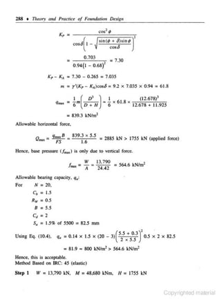
18.0
19.5
2..25
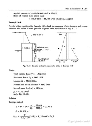
... 75
0
0
0
0
0
0
0
0
7.50
0
0
0
0
0
0
0
0
0
0
0
0
0
0
0
0
0
0
0
0
:1.5
0
12
w
I
day
T
-
DenM
10.0
12.5
15.0
11.5
21.0
0
0
GS
.ae uc
0
0
T
tJU)
c
0
0
0
0
0
0
0
0
0
0
0
0
0
0
0
0
0
0
0
0
0
0
0
-
conlent
uc •
u..
Unc::onlhld
Uquld~
Pl • P1Mic limit
GS • Grein tim
0
0
0
T • Tl1ulol (Wl
c•
Coneolctdon
0
0
0
0
0
0
0
0
0
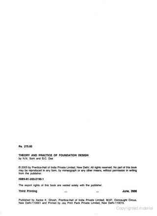
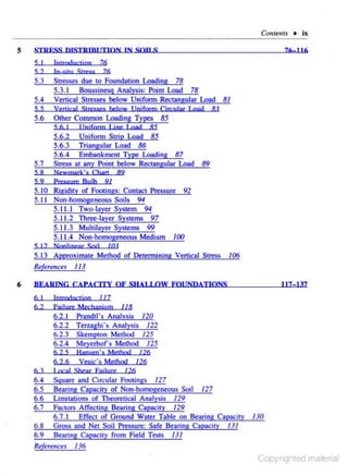
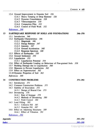
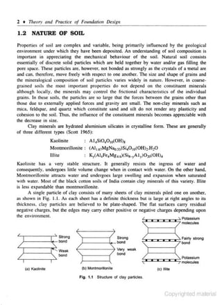
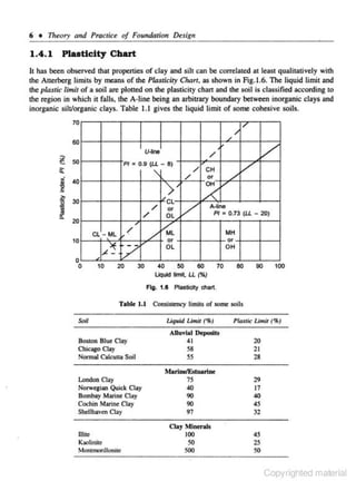
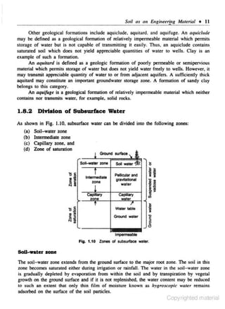
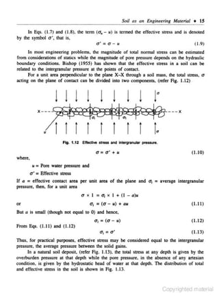
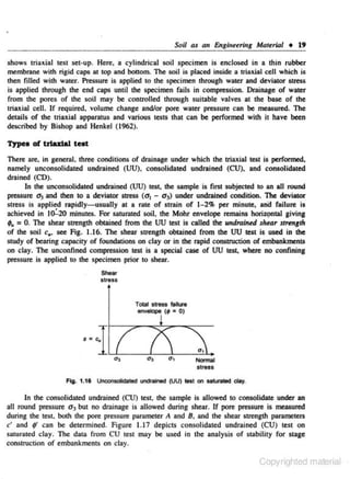
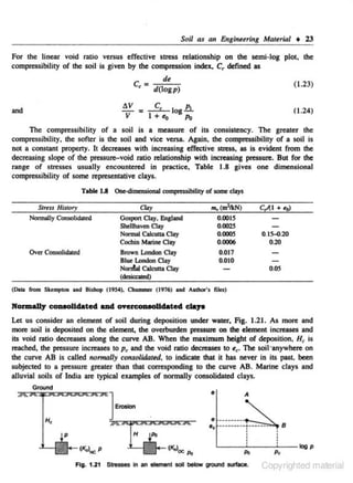
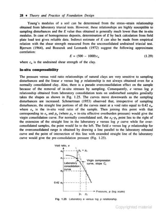
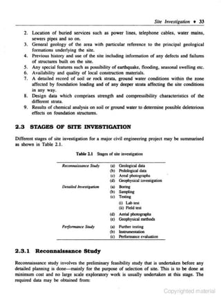
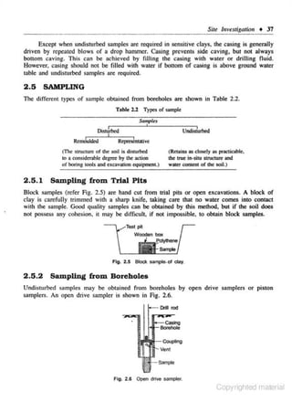
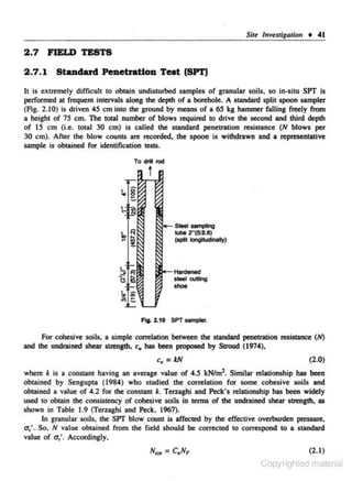
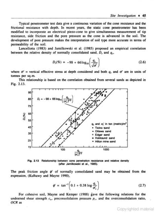
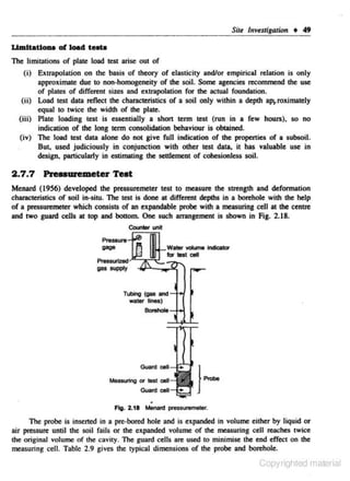
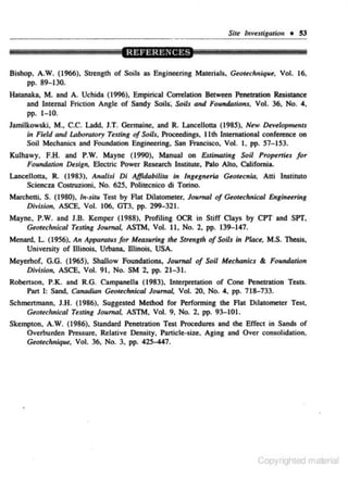
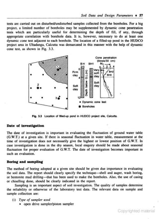
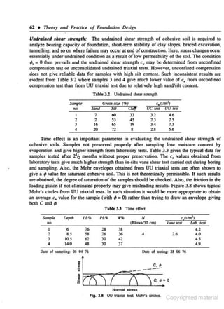
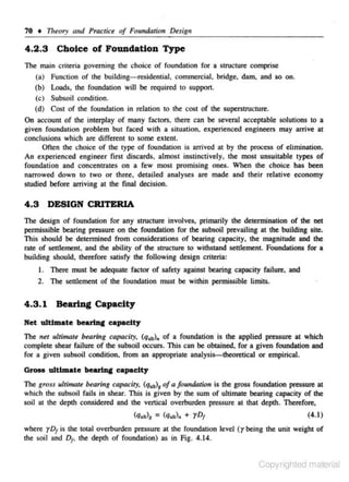
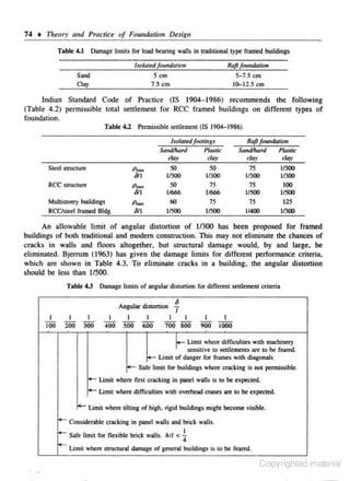
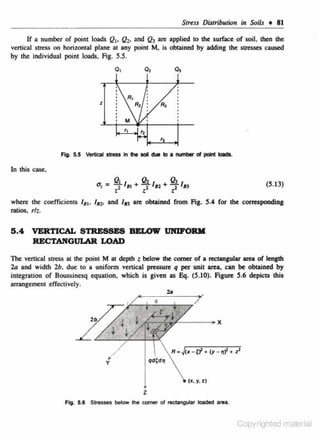
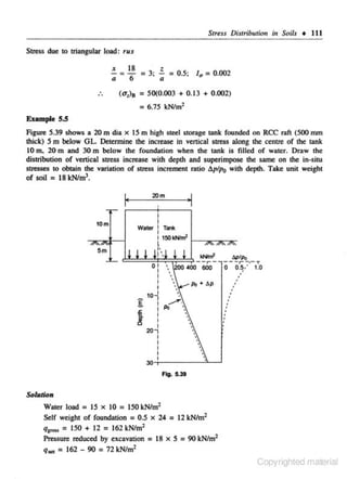
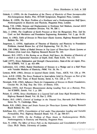
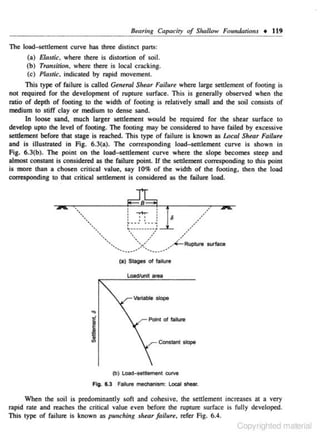
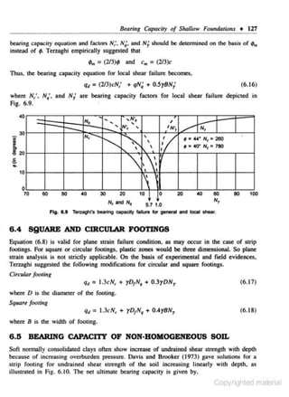
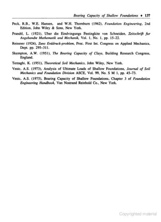
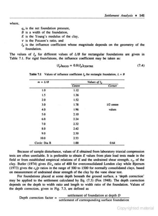
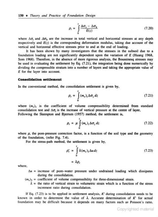
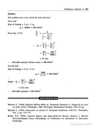
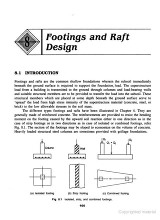
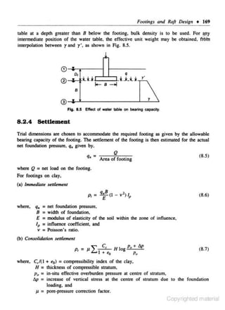
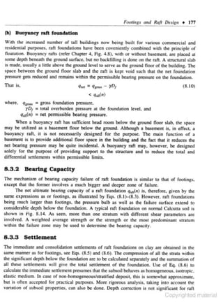
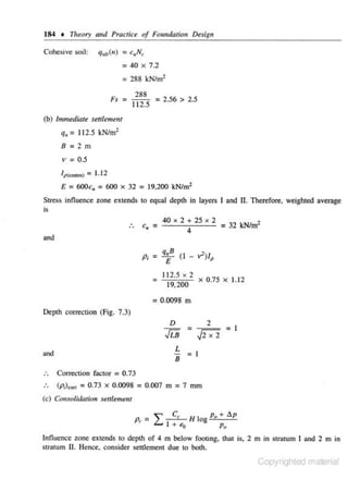
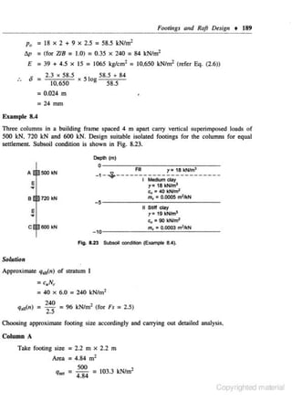
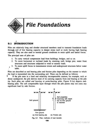
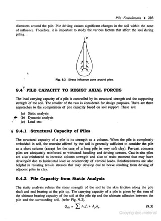
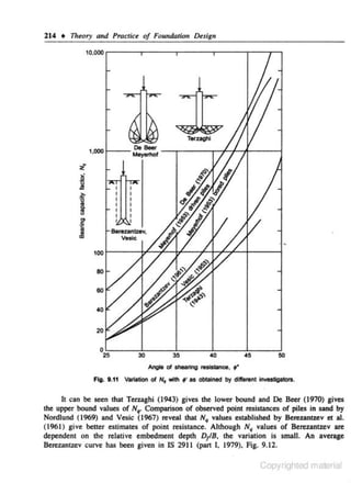
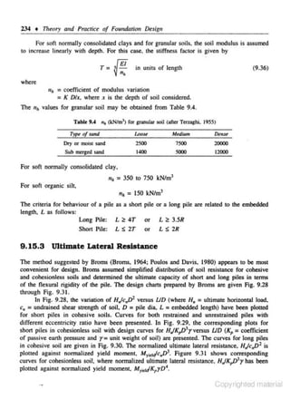
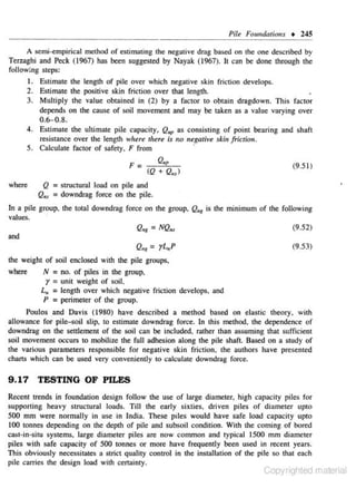
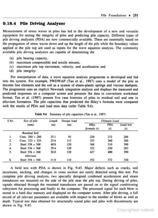
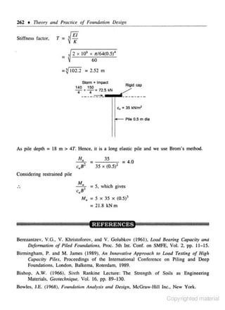
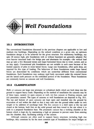
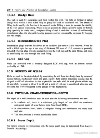
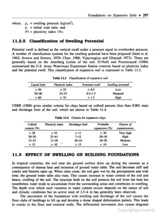
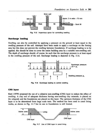
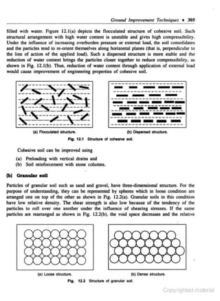
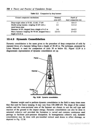
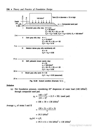
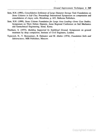
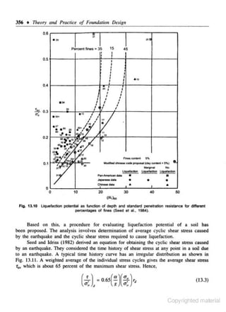
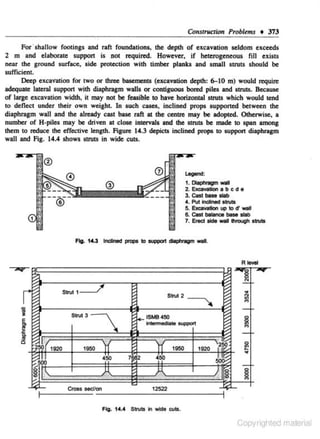
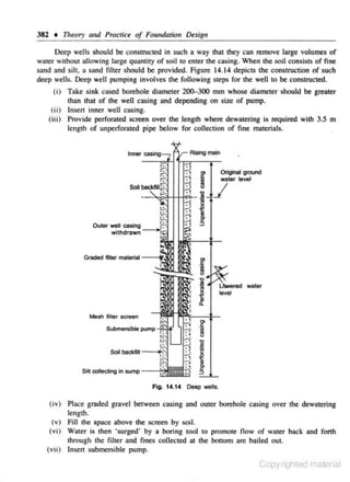
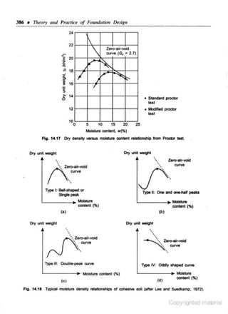
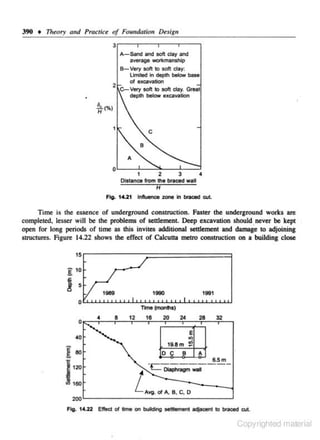
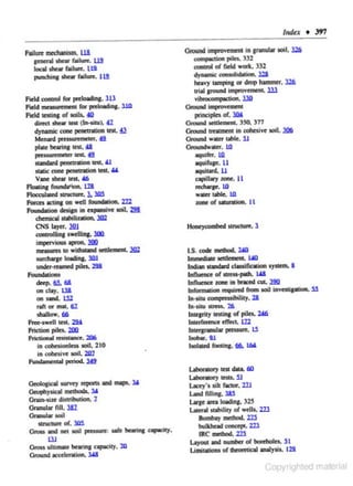
Flg.U -ollobcllobyiMit.
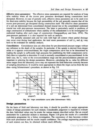
tests should be so chosen ., to give lhe properties of all lhe strata relevant for design. One
should avoid going for unconfined compressioo test in a predomlnandy silty soil.
Similllt'ly. oon.'IOiidation teSt$ are required for cohesive strata only. For sandy strata. one
has to rely more on rield tc5U. such as SPT. Even undisturbed samplu in sand do nor
provide much help.
Soli proftle
Soil profiles should be drawn through a number or boreholes, if not through all of them. to
give the subsoil stratification along a chosen alignment. Such soil profiles dsown for a
number of carefully chosen alignments give a comprehensive picture of the variation of soil
strata, throughout the site. Plotting separately for individual boreholes does 001 cive lhe true •
picture ar a &,lance. Therefore. the best way is to pl01 lhe soil profile on a desired alignment
with nespeet to the vanation of N value with dep<h. The relative consistency of dlffeseot
str.wo emerg<S clearly from sucb a diagram. as depic:tecl throuJb Fla- 3.6.
The position of around water table at lhe time of investiaation should be clearly
indicated in the soil profile. Design or foundations should take appropriate ])OCe of any
seasonal noouation In around water table.
La-.tory tnt data
The lnbor:uory res1 data Qrt given in different fonns in the soil test report. The interpretatjon
t _,,.yrighted ma ,noll

80. 60 • 1?reory and Praclice of Founda#on Design
·w (8Jows/30 em)
0 10 20 30
0
4()
so
.
4
6
g
~
(j
1
1
12
12
16
1
'
2
3
1
'
c--.
24
28
=;
30
Fig.
;1.1 Soli pro4ile
ihrough -
boreholes and SPT data.
or data, thereby becomes difficult. While the basic b:St data should always be there, the
engineer should• be in a position to make proper assessment of the engineering propenies of
different strata to be used for design.
The basic test data may be summariud under the foUowing categories for each major
Stratum of a s-ubsoil deposil:
(a)
Classification data
Bulk density
Natural moisture content
Atterberg limits
Grain-size distribution
(b)
Engin~ering pro~rlit!s
Shear srrength parameters
Penneability
Consolidation test data: m...,
Compaction characteristics
c,.. eli
(c) Chemical and mineralogical data
(d)
Chemical test on water samples
Data Interpretation
The consistency data should be established before choosing the design parameters for a given
problem. Further, the reliability of data and their consistency may be studied qualitatively
from the results of individual testS. For example.
Copyrighted material

81. Soil Data arui IHsign
Parami!IUl t
'1
Atterbera Umits
Grai,..aia:e
Mlneralosr
Classification
Auerbera limits'
Natural moisnue conu:nt
Slandanl peneuation resiSW>Ce (N value)
Undrained
war wenglh
Consolldadon characleristic:s
Cl4st~" t~stt:
A elooe examination or lhe IJ&in·lla:e distributioo dala and lhe
Atterbera limits may reveal incon&Jsu:ney in teSt results. ln Table 3.1 which gi>es a set or
daiA. sample no. 4 wllh clay fncdon or only 8,. indica~e~ a highly plastic clay with
liquid limit 62.. while sample no. S wllh 1 cloy fnctlon 11 biJh 11 48.. bas a liquid limit of
35.. only. These dala do not inspire confidence. It is necessary. ~~~ererore to cheek !he
Atterbera limits against lhe pain·size distribution or eoch sample to determine their
rdiability/eonsistenc:y.
=
Ooulllcaloft ICfU
Tobk 3.1
-
s-pt.
I
2
)
•
s
GroU.·•Iu
S<wJ
7
2
16
20
6
Sili
60
Sl
........!1 , _
u. 1"1 I'L 1" 1
t•!
Clay
.,
sa
))
2M
2&.2
76
u .o
39
72
19
8
62
30.2
46
46
35
2S.O
6S
ConsilttiiCJ: The variation or Atterberg limits and natural moisture conlent with depth
gives a clear indication of the relative consistency
or different
suata. A natural moisture
content cl0$C to the plastic limit and a high bulk density eonfinns a finn to stiff clay whereas
a natural moisture content approaching liquid limit should generally give a lower unit weight
and thus. indicau:s a soft normally consolidated soil, Fig. 3.7.
00
•
T
•
W(~)
y(thn')
. .
10 15
'""
.
20
•I
-.
2
i
'·
e
16a
/.
10
12
II
w
u
1Q edIT'"
a

82. 62 • Theory and Pracriu of Foundation Design
Undrdilltd lhtar strength: The undrained shear strength of cohesive soil is required to
analyze bearing capacity of foundation, shon-term stability of clay slopes, brnced excavation,
runnelling. and so on where fajlure may occur at end of construction. Here. s tress changes occur
essentially under undrained condition as a result or' low permeability or lhe soil. The condition
0 then prevails and lhe undrained shear strength c. may be determined from unconfined
compression test or unconsolidated undrained u-iax.iaJ tesrs. However. unconfined compression
does not give reliable data for samples with high si1r content. Such inconsistent results are
evident from Table 3.2 where samples 3 and 4 give much lower value of c. from unconfined
compression test than from UU triaxial test due to relatively high sand/silt content.
;. =
Tabl< :l.l Undrained shear stttnglh
Somple
c. (tlm2)
Grain-.siu (~~
SoNI
SiJJ
•••
I
ciil!
7
16
S3
6S
4
20
33
4S
19
8
60
2
3
72
z
U~ le-SI
3.2
4.6
2.3
3.4
25
7.3
28
5.6
1J'lJ I~SI
Time effect is an important parameter in eva.Jua1ing tbe undrained shear strength of
cohesive soils. Samples not preserved properly after sampling lose moisture content by
evaporation and give higher Strength from laboratory tests. Table 3.3 gives the typical data for
/
samples tested after 2 1 2 months without proper preservation. The c, values obtained from
laboratory tescs give much higher stre, gth than in-situ vane shear test carried out during boring
n
and sampling. Also, the Mohr envelopes obtained from UU triaxial tests are often shown to
give a ; value for saturated cohesive soil. This is not lheoretically permissible. If such results
are obtained, the degree of saturation of the samples should be checked. Also, the friction in lhe
loading piston if not elintinated properly may give misleading results. Figure 3.8 shows typical
Mohr's cin:les from UU triaxial tests. In such situation it would be more appropriate to obtain
an average c. value for the sample (with ; = 0) rather than trying to draw an envelope giving
both C and;.
Table 3J Time effect
Stnnpl~
lNpth
U 'To
PL'To
WI!>
6
8.5
76
S8
62
28
26
30
48
30
38
36
42
37
no.
I
z
3
4
10.5
14.0
N
(Biowt/30 cOl)
4.2
26
4
4.0
4.5
4.9
O.te of Sllmpling;: OS 04 16
c.,
:!
c
-- ----
"
•
•
..
~
NOfmal stress
Fig.
u
uu
triuial teot Mohfs cirdes.
Copyrighted material

83. Soil Data and
D~sig,
Parameurs
t
63
Efftctiv~ str~ss JHlramd~rs: The effective stress parameters are required for analysis of long
term s tability when all the excess pore pressures developed during const·ruction ha ve
dissipated. However. in ca~ of granular soils. effective stress parameters are to be used even
for short-term stability because me high permeability of lhe soil generally ensures that all the
excess pore-pressures get dissipated during construction itself. The effective shear parameters
of a soil arc determined from consolidated drained triaxial test or the consolidated undrained
rriaxial test with pore-pressure measurement. TI1e latte- is particularly useful in problems of
r
stage constnJction of embankment where stability of me embankment is to be investigated for
undrained loading afte r each stage of construct.i on (Gangopadhyay and Som. 1974). The
pore-pressure parameter A is aloo required for such an analysis.
For purtiaiJy saturated soils and for soils with high silt content where partial drainage
may occur even during load applicaajon, the total suess parameters of soil (c. and ; .,) may
have to be evaluated for stability nnnlysis.
Consolidation: Consolidation tests are often done for pre..detennined press-ure ranges without
any referenc-e to the depth of the samples. In panicular. if the Si'mple is derived from deeper
strata or it appears overconsolidated. the virgin compression curve has to be determined by
loading the sample to sufficiently high pressures for es~blishing the field compression curve.
Only men is it possible to determine if n soil is normally consolidated or preconsolidated. In the
latter case. the Ct' value in the overconsolidation range and the preconsolidation press ure are
important in selecting the design parameters. Moreover. calculating the m., value for different
srrcss ranges from the laboratory curve may not represent the field behaviour correctly because
of sampling disturbances. h would be more appropriate to obtain the virgin curves from the test
data-using Schmcrtm:mn's procedure. as shown in Fig. 3.9.
1.0
0.8
8
e
"
~
·~Po
-"
''
-~
,p,
~
r-...."fiet
0.6
'"'
Lab
0.4
0.1
: p, • 0.9(kglcm')
0.5 1.0
p~cmz)
~
~
5.0 10 20
. ~' J!2.
:
•
•
•
.
•
"'
•
•
•
0. 1
0.5 t .O
' ""
tO 20
p(l<ol<m')
Fig. 3.9 VIrgin c:onsolidalion curYe (after Sc:hmertmaM 1953).
DeaiCD puametezs
On the bas is of field nnd laboratory test data, it should be possible to assign appropriate
values of design parameters for each stratum. Considerable judgement is required to evaluate
the data. Individual values may be erratic for various reasons described earlier. But an over.tll
assessment for a particular stratum is necessary. Figure 3.10 gives the resultS of a controlled
exploration programme for a foilurc investigation. The consistency of data bec.omes evident
from such presentation and the results inspire confidence. The average engineering properties
of each stratum can thus. be obtained without much difficulty.
Copyrighted material

84. 64 • Theory and Practice of Foundation Design
-0
•-
0
0
•- •
0
•
.....: ''
'''
'
Jo '
: '
•
f,
'
'
:--.!
I
i
J
i..
l!
....... ;..
I
.. f-..· - -·d
0
~
e;
~
~
:!
,._
i
i
..
~
·~ J
N
:r
t
n
t:
..
h
u
~!
~
~·
ij
:h
!t
N
i
I
,•, •
fl
0
j
I
I
I
i
"
~
~
~
D
~
!<I
:;:
!:1
II
Iii
Oangopadhyay, C.R. and· N.N. Som (1974). An Approach to ' · = 0 Analy•is for Stage
Constr11ction, Proceedings ASCE, Vol. 100, OT6, pp. 699-703.
Copyrighted material

85. Foundations: Types
and Design Criteria
4.1
INTRODUCTION
Foundation is that part of a structure which provides s uppon to the structure and the loads
coming from it. Thus, foundation means the soil or rock that ultimately suppons the load
and any pan of the structure which serves to transmit the load into the soil. The design of
foundation for a structure, therefore involves the following:
1. Evaluation of lhe capacity of lhe soil to s uppon the loads and
2. Designing proper structural elements to transmit the super structure load into the soil.
Often the term foundntion describes only the structurnl elements but this definition is
incomplete. because the ability of the structural element to transmit the load is limited by the
capability of the soil to suppon the load. Therefore. the problem should be considered .. a
,
whole and not in isolation. A foundation failure may destroy the superstructure as well while
a failure in the superstnJcture might resuJt only in localized damage and does not essentially
mean failure of the foundation.
4 .2
TYPES OF FOUNDATION
Foundations can be classified as shallow and deep foundations depending upon the depth of
soil which is affected by the foundation loading and. consequently. affect the foundation
behaviour. These can be further divided into different types of foundations which are
nonnally 3dOpted in pmctice. This classification is shown in Fig. 4.1.
Foundation
Deep
ShallOw
Ran
Footings
Isolated
Combined
I
PileS
Strip Conventional raft
I
I
Wei/Caisson
Buoyancy raft
Fig. 4.1 Types of foundation.
85
Copyrighted material

86. 66 • Theory atrd PracliG'e of Foundation Design
4 .2 . 1 Sballow Foundations
In shallow fo undations. the load is transmitted to the soil lying immediately below the
substructure. as shown in Fig. 4.2. Such foundations are used when the subsoil near the
ground surface has adequate strength to support the load.
Ground
surface
.
.
•
•
:' lnftuenoe ':
~
zone /
• .
/
•
••
.....-·
'•
Fig . ... 2 Shalow loundatlon.
J.l'oot!D.ga
lso/aJ$d footing:
Isolated footings are provided to support the columns of a building frame
· individually. Figure 4.3 depicts an isolated footing. Such fOOtings behave independently of
each other without being influenced by adjacent footings in any way .
...
...
-rni'F
B
c,
c,
c,
0E
I·
B
·I
Fig. 4.3 lsola1ed ftxltlng.
Combined footing: Combined footings arc designed to support two or more adjacent
columns in a building frame where isolated footings either overlap or come very close to one
another (refer Fig. 4.4).
E""'1_6;"
Az
Ground
surface
x..J
B,
c,
B,
8
1!1-''----fil' '
c,
Fig. •·• Combined toocing.
Copyrighted material

87. Foundations: TyfHs and
D~s;gn Crit~ria
+ 67
Strip footing:
Strip footings support a load bearing wall or a number of c losely spa~
columns in a row. They form a long, narrow continuous foundation, with the width small
compared to the length, as illustrated in Fig. 4.5.
A,
I
I
c,
Flg. 4.5 Strlp
-ng.
Raft or mat fOUIUlaUoa
or
A large number
columns or often~ the entire sttucture is founded on one single slab or
raft. When individual column footings are, together, found to occupy more than 70% of the
plan area of the building, raft fouodations are provided. This is shown in Fig. 4.6. The basic
difference between footings and rafts lies in their size-the latter being mue-h larger and
affecting a greater area of the soil in determining its behaviour.
,--------:1I
I
.I
U
L_ ____!
. Jit!~;:=J[~ =.;:Jt~ dr ~ ~:-r.:
1 X
~
:
Section on-XX
L---------------•
Flg.
u
Raft foundatiOn.
ConventioiUII rq/1:
Conventional rafts are provided at shallow depth beneath the ground
surface and backfilling is done on the raft to reach the original ground surface. Thereaf~r
plinth filling is done tO lay the ground Uoor of the building, as shown in Fig. 4.7.
Gtound
Bodo 111
Raft
Fig. .C.T Conventional raft.
Copyrighted material

88. 68 • Theory and Practiu of Foundotion Duign
BruJy<~.ru:y
raft: Buoyancy rafls are placed at some depth beneath the ground surface but no
backfilling is done on the raft. A ground floor slab is provided at the desired height above
the ground and the space betW<:en the ground floor slab and the foundation raft ;. kept void,
refer Fig. 4.8, to provide relief of overburden pressure at the foundation level. Basement
rafls are typiC11l examples of buoyancy raft foundation.
Gould
"f'
V
0
I
D
Fig. 4.1 ll<Joyaney raft.
4 .2 .2
Deep FoundatloDa
In deep foundations. tbe load is transmitted well below the bottom of the subsuucture, as
shown in Fig. 4 .9. Deep foundations are provided when soil immediately below the structure
does not have adequate bearing capacity but the soil at deeper stralll have.
Grcund
I
I
I
I
I
+
t
I
I
I
I
',' ___.,
I
I
I
lnftuence zone
I
/
/
Fig. 4.1 Deep -
·
Pile foundation
Piles transfer the load lhroogh soft upper strata either by end bearing on hard stratum or by
friction between the soil and the pile shaft and are accordingly called end bearing piles or
friction piles, Fig. 4.10.
t
+
t
+
Ann to
sUff day
t
t
t t
t t
t
(a) Frlcrlon pile
Soft
Clay
Rod<
(b) End bearing pile
Fig. 4.10 Pile foundations.
Copyrighted material

89. Foundations: Types and Design Criteria • 69
Usually a column load is supponed on a group or piles through a pile cap. as shown
.
0
in Fig. 4.11. Rafts and piles are sometimes combined 1 form a piled rafl illustrated in
Fig. 4.12.
0
0
ot
ol
to
to
CaOJmn
r:!:1:PVe
r
0
0
Pile"
cap
Plies
0
0
0
0
0
0
0
IH±::f::::>,..,
Pies
0
FlO. 4.11 Pl'le foundollon.
U..J...H1T> Plies
Hard SOil
Fig. 4.12 Piled raft.
Piers IUld caiseou
These arc large diameter piles, in effect. which are used to suppon heavy structural load
from bridges or very tall multistoreyed buildings. A pier or a well is a shaft drilled into the
soil which is then filled with concrete, gravel, and so on. The bottom of the shaft may be
undercut or belled out. either by hand or machine as depicted in Fig. 4.13 to afford a large
bearing area. Wells are rigid structural elements and can take large lateral forces while piles
are slender and liable to bend under flexural stress. Cais.Cions are large diameter wells which
are installed by special construction technique.
f9
• HFL
Rmr bed
I
Caisson
Well fourdatlon
Fig. 4.13 caisson and well foundation.
Copyrighted material

90. 70 • Theory and Practice of FoundaJiorr De.sign
4 .2.3 Choice of Foundation Type
The main criteria governing the choice of foundation for a struc.ture comprise
(a)
(b)
(c)
(d)
Function of the building-residential, commercial, bridge. dam. and so on.
Loads, the foundation will be rc<juired to support.
Subsoil condition.
Cost of the foundation in relation to the cost of the superstructure.
On account or the interplay of many factors. there can be several acceptable solutions to a
given foundation problem but faced with a situation, experienced engineers may arrive at
conclusions which are different to some extent
Oftc.n tile choice of the type of foundation is arrived at by the process of elimination.
An experienced engineer first discards, almost instinctively, the most unsuitable types of
foundation and conc.entrates on a few most promising ones. When the choice has been
narrowed down to two or three, detailed analyses are made and their relative economy
studied before arriving at the final decision.
4.3 DESIGN CRITERIA
The design of foundation for any StiICture involves. primariJy the determination of the net
permissible bearing pressure on the foundation for the subsoil prevailing at the building site.
Th_ should be detennined from considerations of bearing capacity, the magnitude and the
is
rote of settlement, and the ability of the structure to withsrand settlement. Foundations for a
building should, therefore satisfy the following design criteria:
I. There must be adequate factor of safety against bearing capacity failure, and
2. The settlement of the foundation must be within permissible limits.
4 .3 . 1 Bearing Capacity
Net ultl.mate bearlJIC capacity
The net 1dlimare bearing capacity, (qutJ,. of a foundation is the applied pressure at which
complete shear failure of the subsoil occurs. This can be obtained. for a given foundation and
for a given subsoil condition. from an appropriate analysis-theoretical or empirical.
a...,.. ulttmate bearlJIC capaclty
The gross ultimate ~aring capacity, (q.IJ1 of a found.Oiion is the gross foundation pressure at
which the subsoil fails in shear. This is given by the sum of ultimate bearing capacity of the
soil at the depth considered and the vertical overburden pressure at that depth. Therefore,
(q,,,>, = (q.,,l. + rD1
(4.1)
where yD1 is the total overburden pressure at the foundation level (ybeing the unit weight of
the soil ond D , the depth of foundation) as in Fig. 4. 14.
1
Copyrighted material

91. Foundalio11s: Types curd Design Criteria • 71
FJg. • .14 Gross and net ultimate bearing capacity.
Allowable
bearl.aC capeclty
The allowable bearing capacity of a foundation is the muimum allowable net pressure on
the foundation deccrmined from considerations or shear failure of the ground. This is
obtained by dividing the net ultimate bearing capacity by a suitable factor of safety. that is,
qau- (q,ul,
F
where. F = factor of safety.
The determination of allowable bearing capacity of a foundation from shear failure
consideration involves a bearing capacity analysis of the foundation with the relevant soil
propenies and the choice of an appropriate safety factor.
A factor of safery is applied on the ultimate bearing capacity of a foundation to
safeguard against:
(i) natural variation in the shear strength of the soil.
(ii) uncertainties in the accuracy of test results to detennine shear strength.
(iii) uncenainties in the reliability of theoretical and empirical methods of determining
bearing capacity.
(iv) excessive yielding of the foundation when the soil apprOOches shear failure.
Of the above. narural variation in subsoil propenies and uncenainty about the accuracy of
test results are the primary reasons for requiring an adequate factor of safety in determining
the allowable bearing capacity of a foundation. Subsoil propenies
a1
a site by their very
nature, are heterogeneous and there is usually wide variation of rest resultS. Therefore. a high
degree of judgement is required in selecting the shear strength parameters for design. Any
general guidance in thjs regard is neither possible nor always desirable. but a safety faclOr of
2.5- 3.0 may be adopted to guard against the variations and uncertainties listed above. Lower
factor of safety, say, 2.0 may be adopted for a temporary construction or on sites where
subsoil condition is well known and uniform. Lowering the factor of safery even funhet may
lead to locaJ yielding and excessive shear deformation of the soil.
The first step in a foundation design is to determine the net allowable bearing capacity, as
described above. It would, then be required to estimate the selllement of the foundation for a
bearing pressure equal to the net allowable bearing capacity and then to see if the estimated
seulemcnr is within the permissible Umirs. lf not, lhe foundation is to be redesigned.
4 .3 .2
The Settlement Criteria
Let us consider the columns in a building frame which were originally at the same level but
have settled differentially after application of the building load, illustrated in Fig. 4.15. The
different settlement criteria c:Jn then be stated as:
Copyrighted material

92. 72 + Titeory and Practice of Foundation Design
(a) MaJ<imulT settlement, p=,
(b) MaJ<imum differential set~ement, A
(c) MaJ<imum angular distortion. 8/1
Original level
offoundotion
-:...._
-:•
4-
Fig. 4. 15 Settlement of foundation and setUement criteria.
All these criteria can be evaluated from an adequate settlement analysis of the foundation.
However, it is obvious that mere prediction of settlement is only of limited practical value
unless some idea about how much settlement the building is going 10 tolernte without suffering
damage. is obtained. If a building frame settles uniformly over its area. no matter by whatever
amount. it has no adverse effec.t on the behaviour of its stnJc.tural components. Maximum
settlement is important in relation to access and services of the building and is generally of not
much significance when it is within reasonable limits. Damage to suuctural components may.
however. occur if there is excessive differential settlement.
Damages due to differential settlement may be classified under the following categories
(Skempton and McDonald 1955),
(i) Structural damage involving frame members. namely, beams, columns, and their
joints.
(ii) Architectural damage involving the walls, floors, and finishes.
(iii) Combined structural and architectural damage, and
(iv) Visual effects.
Building frames are generally designed 10 achieve uniform ~ttlement.
Since differential seulement occurs in most cases, secondary stresses are induced in the
members of the framed structure. the evaluation of which is yet to become a 5tandard
practice. althougb with the advent of numerical analysis using computers, it is now possible
to undertake theoretical analysis of complicated buiJding frames for different conditions of
total and differential settlement.
In steel frames, local failure may be prevented by yielding of the joinlS, provided mild
stoel is used because the relative rotation required to cause fracture is in most cases greater
than that which can occur. However, with increasing use of we1ding in recent years.
secondary stres.ses are of greater importance since yielding of welded connections would
result in rupture and failure.
SlnlctMral dalftDge:
Architectural damage: This refers to cracks in the wal1s. floors. and finishes which is
apparently a more immediate effect of differential seulement than the overstressing of
structural members. Excessive c- acking may cause damage to the functional aspects of the
r
building. For example, major cracks are considered detrimental to hospitol buildings, cold
storage, und the like. Hence., in most cases, the cracks or the architectural damages are the
guiding fac tor in de-ermining the allowable se.ulement of buildings.
t
Copyrighted material

93. Foundations: Types and Design Crireria • 73
Co...biMd tudrilutura/ and strudluvl t/4maf.: Usually. archileetural dAmage occur1> long
before there is structural damage in beams and columns and consequently a stn>Ctural damage
is almost invariably accompanied by architectural damage.
VlsiUII efful: Even before there is any architectural or structural damage. excessive
differen1ial settlement or tilt which can he recognised by naked eye cannot he accepted either
psychologically or aesthetically.
Allowableeettlemeat
The allowable settlement of a building can he determined from an integrated analysis of the
building frame for given magnitudes of settlement. This is, however, laborious and time
consuming and has to he done separately for each building. Therefore. attempu have been made
to estimate the allowable settlement from statistical correlation between damage and settlement
criteria.
The allowable settlement of buildings depends upon the type of con$11Uction, the type
of foundation, and the natwe of soil (sand or clay). The angular distortion appears to he the
more useful criterion for establishing the allowable limits. Terzaghi (1938) studied the
settlement pattern of a number of brick walls in Vienna. He found that the walls reached
their ultimate strength when the angular distortion was 1128S and concluded that an average
settlement of S-7.5 em woold be considered normal.
Skempton and McDonald (19SS) derived a statistical correlation between damage and
settlement of 98 buildings from different partS of the world and coocluded that an angular
distortion of 11300 should be considered the allowable limit for conventional buildings.
Jappeli (1965) obsaved the damages to a three-storeyed building on clay due to differential
settlement and confirmed that an angular distortion of greater than 11300 would lead to
severe damages in walls of ordinary buildings. Whitman and Lambe (1964), on the other
hand, studied the settlement pattern of buildings in MIT Campus and observed that an
angular distortion of as little as 11800 was sufficient to cause cracks in bricks and masonry
elements. Mackinley (1964) made a study of more than fifteen structures damaged by settlement. He observed that there was no simple rule to define the tolerance of structures to
settlement. A cement silo had collapsed in New York after ortly 5 em of differential settlement whereas some public buildings in Mexico City had been in u.c;e even after differential
settlement of more than 10 em.
Rethatl (1961) carried out an investigation of twelve buildings on fill. This time. the
rigidity or the structure as represented by the number of storeys was also considered. While
the critical angular distortion of 11300 agreed well with those proposed by Skempton and
McDonald, it was found that 91% of the buildings that suffered structural damage were two
storeys or lower. Hence, the author concluded, the critical angular distonion should he
related to the rigidity of the building. Some funher studies on allowable settlement have been
made by Feld ( 1964) and Grant et al. (1974).
While much work still remains to he done on the subject to recommend some readily
acceptable values of allowable settlement. it seems there is a common agreement that an
angular dis tortion of more than 11300 may lead to damages in conventional load hearing wall
and framed construction. There is, as yet, no agreed guideline as regards the allowable
maximum settlement of a building. Skempton and McDonald (1955) have proposed some
tentative damage limits which are shown in Table 4.1.
Copyrighted material

94. 74 • 111eory and Practice of Foundation Design
Tab~
Damage limilS for load bowing walls in tr.ldilional cype framed buildings
4.1
IsoJa1~d formdation
Raft fotmdalion
S em
S-1.5 em
1~12.5 em
Sand
Clay
7.5 em
Indian Standard Code of Practice (IS 1904-1986) recommends the following
(Table 4.2) permissible total settlement for RCC framed buildings on different types of
foundat ion.
Tablt 4.2 Pcnnissible ~ulcment (IS 1904-1986)
lsoJ<~trd footings
SamJ/hard
day
Sttt'l structure
day
50
75
75
11666
11500
60
75
75
11500
cS'I
75
11300
1
1666
"'-
so
11300
50
cS'I
Po...
cS'I
MuJtistorey buildings
RCO.O.eel fr:uned Bldg.
Pllutic
11300
Atu~~.
ROC SUIC:IUte
Raft jOtln.dalion
SaNl/h4rd
PlasJk
day
day
11500
11400
11300
11300
100
1/500
125
11300
An allowable limit of angular distortion of 11300 has been proposed for frnmed
buildings of bolh traditional and modern coosltuc.tion. This may not eliminate lhe chances of
cracks in walls aod floors altogether, but structural damage would. by and large, be
eliminated. Bjcrrum ( 1963) has given the damage limits for different performance criteria.
which are shown in Table 4.3. To eliminate cracks in a building. the angular distortion
should be less than 11500.
Table 4.3 Damage limits of an&ular distortion for different ~ttlemc:nt criteria
6
Angular distortion
I
I
I
2oii 300
100
I
400
I
500
I
600
I
I
I
700 800
I
900
I
iOOO
~
~
Umit "''here difficulties with m.achinery
sensitive lO settlements a.re 10 be feared.
f.- Limit of danger for frames with diagonals
Safe limit for buUdin.gs v.'here cracking is not pennissible.
,.._ Umit where first aacking in panel walls is to be: expocted.
,.._ Limit where difficulties with overhead cranes are lO be expected.
~ Umit where tilting of high. rigid buildings might become visible.
f+- Considerable cracking in panel w-aUs and brick walls.
~ Safe limit for flexible brick waJJs.
-
h/1 <
~
Umh where st:ructural damage of general buildings is to be feared.
Copyrighted material

95. Foundations: Types and Design Cn'teria • 15
Net permiaolble
bearlD& preosure
The net pemUssible bearing pressure on a founda1.ion is to be determined from considerations
of safe bearing capacity and permissible seulement, so as to satisfy both design c riteria.
Starting with the net allowable bearing capacity. if the estimated settlement' appears to go
beyond the permissible limits, the bearing pressure should be correspondingly reduced until
the criterion or allowable settlement is also satisfied although this may mean a higher factor
of safely against bearing capacity failure. For soft clays. in generaJ. the settlement ~riterion
governs the choice of net permissible bearing pressure. This is particularly so for raft
foundations.
Bjcrrum. L (1963), Relation /Mtwun Obstressed and Calculated Settlement of Structures iJr
Clay, and Sand, Norwegian Geotechnical Institute Bulletin, Oct 1969.
Gnmt, R .. J.T. Christian, and E. Van Man:ke (1974), Differential Smlement of Buildings.
Proceedings ASCE, Vol. 100. GT9, pp. 973-991.
I.S. 1904 ( 1986), Code of Practice for Design of Shallow Foundations, Bureau of Indian
Standards. New Delhi.
Jappeli ( 1965), Settlement Studies of Some Struct11res in Europe, Proceedings 6th International Confere.nce on Soil Mechanics and Foundation Engineering, Vol. 2,
pp. 88-92.
Rethati (1961), Behaviour of Building Foundations on Embankments. Proceedings 5th
ICSMFE, Vol. I , p. 781.
Skempton, A.W. and D.H. McDonald (1955), A Survey of Comparison Between Calculated
and Observed Settlmrent of Structures in Clay, Proceedings Conference on Correlation
of Calculated and Observed Stresses and Displacement of Structures, Institute or Civil
Engineers, London, Vol. I, p. 38.
Terzaghi. K. (1938), Settlement of Structures in Europe and Met/rods of Observation,
Proceedings ASCE, Vol. 103, p ..J432.
Whitman, R.V. and T.W. Lambe (1964), Soil Mecha11ics. McGraw-Hill Publicatjon,
New Yorlc..
Copyrighted material

96. Di~tribution
Stress
Soils
in
5 . 1 INTRODUCTION
An essential step in foundation design is to determine the magnitude and distribution of
stresses that are develOped in the soil due to the application of structural load. It is these
stresses which not only cause settlement of the foundation but determine its stability against
shear failure.
The stresses and strains in soil mass depend on the stress-defonnation characteristics.
anisotropy and non·homogeneity of the soil. and also on the boundary conditions. But the
task of analyzing stresses tWng all these fac10rs into consideration is extremely complex and,
therefore, the attempts that have been made to date are based on simplifying assumptions.
The most widely used method of analysis is based on the consideration of soil as
homogeneous. isotropic. elastic medium.
It is well understood that the assumption of linearity of the stresHtrain relationship
which fonns the basis of elastic behaviour i- a questionable s implific-ation because soils in
s
their behaviour are ~ntially non·linear. No other widely acceptable theory )las yet been
developed for pnoc. ical use to describe the response of soils to stress changes. Also within the
t
comparatively sman range of stresses that are normally im.p<>sed by structural loads, the
assumption of linearity. for most soils, may be considered to be reasonably valid. Also.
lintlted field evidence reported by Plantema (1953) and Turnbull et al. (1961) show that
measured stresses correspond fairly well to those predicted by elastic theory. Therefore,
refinement of the methods of stress analysis based on the theory of elasticity-still assuming
the validity of lhe linear stress-strain relationship, but taking into consideration the variations
of properties within the soil mass-has often been attempted.
5 .2 IN-SITU STRESS
The stresses in the subsoil due to the over burden are called
Figure S.l shows the in-situ sU'esses in a soil element at a depth
Tota.J vertical stress,
where.
<T
.,
= yz
in ~ situ
z.
or geostatic stresses.
below the ground surface,.
(5. 1)
r = unit weight of soil, and
z = depth below ~ound surface.
71
Copyrighted material

97. Stress Distributio11 in Soils • 77
z
h
Flog. 5.1
In-situ strasses in sol.
(5.2)
Total horizontal stress,
where, K is the coefficient of 1atc- al pressure at rest with respect to total stress.
r
uo
Pore warer pressure,
=Ywh
(5.3)
where. y., = unit weight of water, and
lr = deplh of rhe poinl below warer table.
a =~ - uo
:
Effective verticaJ stress,
"·•
Effec.tive horizontal stress,
= rz - r..h
=~
...,"-uo
= Kyz - Ywh
(5.4)
(5.5)
where K0 = coefficient of eanh pressure at rest with respccl to effec.tive srress.
The value of K., depends on the type of s.oiJ and its stress history. For normally
consolidated soils. it varies from 0.4-0.7. For over consolidated soils. K., depends on the
overconsolidation ratio and generally becomes greater than 1 for overconsolidation rotio
exceeding 4 (Som 1974).
Some empirical formulae for computing K0 values for soils are as follows:
For sand and normally consolidaled clays, laky (1944) gave a relationship berween K. and
!he angle or shear resistance, ~.
.
K11 = I - sin4f
(5.6)
This was subsequently modified by Brooker and Ireland (1965) as
K.
= 0.95 -
(5.7)
sin••
For overconsolidared soils, Alpan (1967) gave rhe relalionship,
( K.Joc
=
(5.8)
(K.)NC (OCRl
where A is a facror depending on rhe plasticiry index of !be soil and is given by
1, = -281 log(l.85A)
(5.9)
Ladd (1977) suggested !he value or 0.41 for A.
Copyrighted material

98. 78 + 111eory and Pra.clice of Foundation De.sign
5.3 STRESSES DUE TO FOUNDATION LOADING
It is generally assumed. in determining the st:rtSSes bene-ath a foundation. that the soil behaves
as an elastic medium (i.e. linear and reversible stress-strain relationship) with identical
properties al all points and in all directions. Allhougb. in practice. a soil can hardly be
approximated to suc.h an ideal medium. the mathematical soJution to this problem was the
only one available to engineers for a very long time. Since the principle of superposition
holds for such a medium. it has been possible to use these results to detennine the stresses
and deflections caused by loads applied over finite areas on lhe surface. Love (1923) gave
equations for stresses and deOec tio~s caused by a loaded circular rigid plate and Newmark
(1942) derived the expression for the s tresses under the comer of a unifonnJy loaded
rectangular area. The tables and charts prepared by Newmark and laler by Fadum ( 1948) are
extensively used to calculate the vertical stresses beneath a fou ndation. The case of a
uniformly loaded strip was solved by Carothers (1920) and 1urgenson (1934). Bishop (19S2)
used stress functions and relaxation technique to calculate the stresses in and underneath a
triangular dam. The most comp)ete pattern of stresses, strains and deflections beneath a
uniform circular load on a homogeneous half space can be obiJlined from tables prepared by
Ahlvin and Ulery ( 1962). From all lhese results, il can be seen lhal the vertical s1resses in a
homogeneous, isotropic elastic body is a function only of lhe dimensions of the loaded area
·and independent of the elastic properties of the soil. However, this is not true in case of the
lateraJ stresses and displacements.
5 .3.1
BouaslDeaq Analysis: PolDt Load
Boussinesq (1985) (sec Terz.agbi 1943) was lhe first 10 obtain solution for the slresses and
deformations in the interior of a soil mass due to a vertical point load applied at the ground
surface, refer Fig. 5.2. He considered the soil mass as a half spoce bounded on lhe top by a
horizontal plane (ground surface) and extending to infinity along ~.pth and width.
.
••
/ y
••
R
y
z
Fig. 5.2 Stress In the soil due
to poin1 IO&d a1 surlaee (rectangular c:ocrdinatos).
Copyrighted material

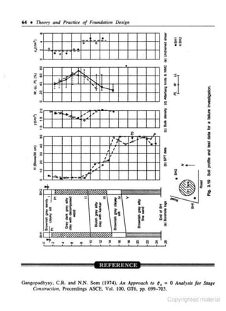
99. Stu.ss Distribution in Soils • 19
Considering soil as a homogeneous, isotropic, and elastic medium, Boossinesq obtained
the expressions for stresses at a poinl (x, y, .t) located at a distance, R from the origin of
coordinates which is also the point of application of the vertical load. Q.
The stress componcnls in Cartesian coordinales are given as:
2
u,
=3Q [y'z
2lr R' -
l-2v{
3
I
~1 =
'
Here,
3Q
2~r
z }]
(2 R +z)x
(R + z)' R3 + R3
- R(R+t) + (R +l)'R' + R'
a~ =
'fx~
+
z}]
(2R+ zll
3Q [ x'z
l-2v{
I
<>x = 2~r R' 3 - R(R + l)
3Q z'
-21< R'
3Q xz1
= -2Jr R'
[.xyz _ 1- 2v {<2R + z).xy}]
3
R'
(5. 10)
(R+ z)'R'
1
R = J<x' + y' + z ) and
v = Poisson's ratio of the soil
h may be observed !hal the vertical slreSs is independent of bolh the stress-strain mndulus
and Poisson's ratio. The lateral stresses and shear stresses. however. depend on Poisson's
ratio but even these are independent of stress-strain mcxlulus. Values of v = 0.5 for saturated
cohesive soils under undrained condition (no volume change) and 0.2-0.3 for cohesionless
soils. are genera11y valid.
In cylindrical coordinateS, !he stress components (refer Fig. 5.3), are:
y
z
"•
Fig. 5.3 Stresses in the aoil due to poin.t load at surface (cylindrical coordinates).
Copyrighted material

100. 80 +
111~ory
and Practice of FoundaHon Design
The stress components in cylindrical coordinates arc written as:
3Q •'
(}'. = - 21r R'
u=
[
Q 3tr·
'
21r R'
1-2v
R (R + z)
]
(5. 11 )
I
2]
Q
a, = ii<(l - 2 v) [ R(R+ t) - ?
3Q t 2r
21r R'
The above expressions for stresses are valid only at distances, away from the point of
load application. At the point of load application, the stre:s..~s are theoretically infinite.
For foundation analysis, the venical stresses on horizontal plane (uJ are mostly
required.
Puuing
= J<x' + y' + t 1 )
R
U,=
where Ill
=
=
J<r' + z1 )
-Q I,
,·
,-
(S. I 2)
3
21r[l+(rill'J'"
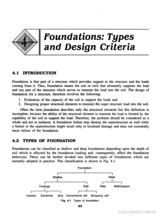
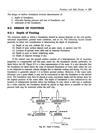
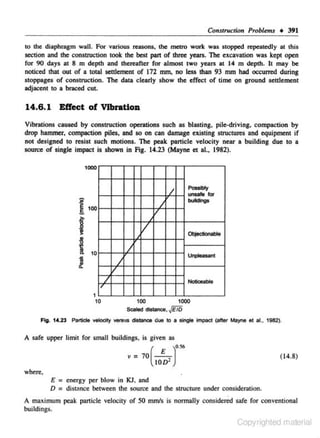
Ill is the influence coefficient for vertical stress at any point within the soil mass. for the
Boussinesq problem. The vaJues of /8 for different values of rlt are given in Fig. 5.4.
0
'
•
l:'
A
0.5
r
• ·- -~· -
-.......
0.4
0
(u, }" = 2 Is
0.3
z
'•
"' """
0.2
0.1
0
0
0.2
0.4
0.6
0.8
r--1.0
1.2
1.4
rtz
FliJ. 5.4 Str.,. Influence fO<Wr for point load
(Boussl~).
Copyrighted material

101. Stress Distribution in S<Jils • 81
If a number of point loads Q1, Q,. and Q3 are applied to the surface of soil, then the
ven.icaJ stress on horizontal plane at any point M, is obtained by adding the stresses caused
by the individual point loads. Fig. 5.5.
o,
l
Fig. 5.5 Venlcal S1noU In ... sal duo 1D 1 rumbor ol point loocll.
In this case.
u,~ ~I11 +~I12 +~I83
z
z
z
(5.13)
where the coefficients I 8 1• I 81• and In are oblllintd from Fig. 5.4 for the eonesponding
ratios. rl;..
5 .4
VERTICAL STRESSES BELOW uNIFORM
RECTANGUlAR LOAD
The venieal stress at the point M at depth z below the comer of a rec~angular area of length
2a and width 2b, due to a uniform vertical pressure q per unit area, can be obtained by
integration of Boussinesq equation. which is given as Eq. (5.10). Figun: 5.6 depicts this
arrangement effectively.
y
(11, )1, Z)
z
Fig. 5.& Stresses below the comer ol rectangular lOaded area.
Copyrighted material

102. 82 • Th.ory and Practice of Foundation Design
The equivalent point load on the infinitesimal area dx dy is given by dQ = q dx dy
The vertical stress at M due to point load dQ (Eq. 5.12)
da, = 3dQ
•'
2>< [I+ (rll)'f12
(5.14)
Integrating Eq. (5. 14) between [- a to +a) and (- b to +b) along the x and y directions
respectively we get,
(5.15)
Evaluation of this double integral gives the general expression fo.r vertical stress at any
point within the soil mass. Let us now consider the vertical stress at the origin (x = y = 0).
Then,
_
O'z(00, l ) ,
2q(
"
2
2
2
abz(a +b +2z
(~+ z )(b
2
2
2
2
)
+ SID -t
•
2
2
+ z )Ja + b + z
ab
)
2
Ja' + .' Jb +
2
( !6)
5.
z
Now taking one quarter of this expression, the vertical streSs below the comer of a
fledble rectangular area (a x b) (i.e. one quarter of the original rectangle 2a x 2b) is
obtained as
where m=
a
l
or
andn=
b
l
(5.18)
where
1(1 is called lbe streSs influence coefficient and is a function of two dimensionless parameters
m and n.
The value or Ia ror different values or m and n are given by Fadum (1948), are shown
in Fig. 5.7.
Copyrighted material

103. Stress Distribution m Seils • 83
m
Fig. 5.7 Influence factor for vertical str8$.S below comer of rectangular lOad, Factum (1948).
5.5 VERTICAL STRESSES BELOW UNIFORM CIRCULAR LOAD
Fo11owing the same principle of superposition as for rectangular load, the venical StreSSeS
below a uniformly distributed circular load may be obtained as in Fig. 5.8.
Copyrighted material

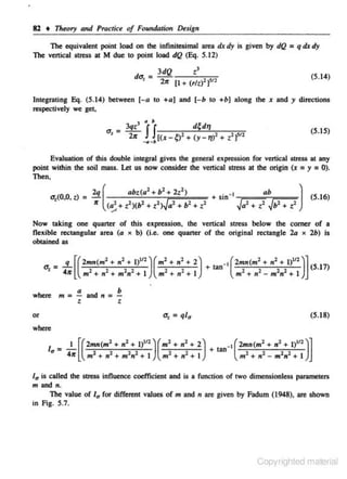
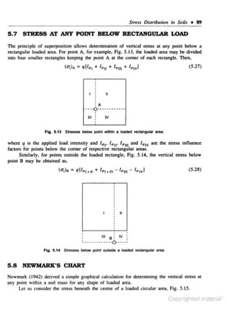
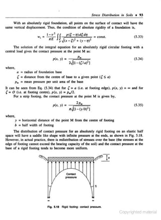
104. 84 • Tlteory and Proctic• of Found<Jtion Design
!!I.
Ckde
q
!&.
1 dia2b 0.2 0.4 q 0.6 q 0.8 1.0
0
./
---1..
1
q
/
/ ~
2
z
i
q
·/
3
1.2
I
•
5
8
7
8
flO. 5.1 -
·--
~ unilonn -
load.
The load on infinitesimal area rd rt/8 is given by dQ = q rdrd8. Also,
R = (,.l + b 2+
r'- 2br cos9)1n
Integrating over the circular area,
II[r +
J alJr
u, = Jqz
2t
=
1
0 0
rdrd8
b2 + z2 - 2brcos8)512
(5. 19)
{A - 1f~n' +n(I+ t)' [ n' +- (I + r•) E( k) + .!..=..!.llo(k p>
n' I
]}
q
I + t
,
12
(5.20)
where E{k) and n 0(k, p) are complete elliptic integrals of the second and third kind of
modulus k and parameter p.
t = ria
= I
n = <Ia
k' =
A =
4t
n 1 + (1 + 1) 2
I
2
if r<a
if r=a
=0 if r >a
For the special case of the points beneath the centre of me load, r = 0
Copyrighted material

105. Stress Distribution in Soils • 85
--·--=--=-}
(a,),.o = q {· [I + (all)'J"'
(S.21)
The vertical s-tresses beneath the centre of a uniform circular load are shown in
Fig. S.8. The stress influence coefficient for a circular loaded area for different values of
ria and tla is given in Appendix A.
5 .6
OTHER COIIIMON LOADING 'tYPES
5 .6 . 1 UDiform Lille Load
The vertical stress in the soil due to a line load p per unit length, applied at the surface is
given by
<1
;
=- 2p
It
=
~·
(S.22)
(x' + ~'>'
~(K(I+:2 /~ 2 )2 )
The stress distribution directly beneath the load {x = 0) is shown in Fig. S.9(a). The
variation of a,j(ph) with xl~ is shown in Appendix A.
0.8
0.7
0.8
0.5
.!!Lo
pl z
·•
0.3
0.2
0. 1
r-.....
z
1.0
5 .6 .2
2.0
3.0
•
{a)
Fig.
J(
{b)
u
Vef1ical · - · In the soli duo to . . . . lood.
UDiform Strip Load
The vertical slresses in the soil due to a uniformly distributed strip load is given by the
expression,
Copyrighted material

106. 86 • Theory and Practice of Foundation Design
q
•
tr
•1
t
•
t
- - - tan 1 - - -
()
x+a
[ ( -)
x a
a. = - tan
2?2]
2at(x - t - - a )
.,
,
(xl+ z-- a1)2 + 4a2x.
(S.23)
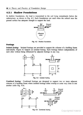
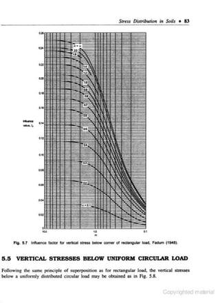
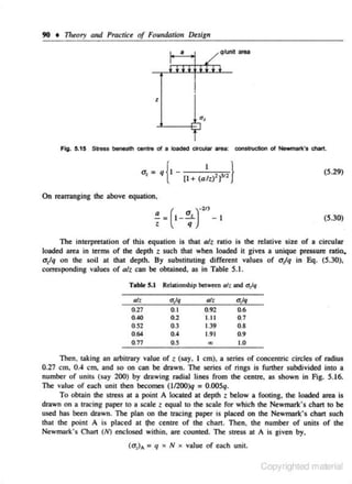
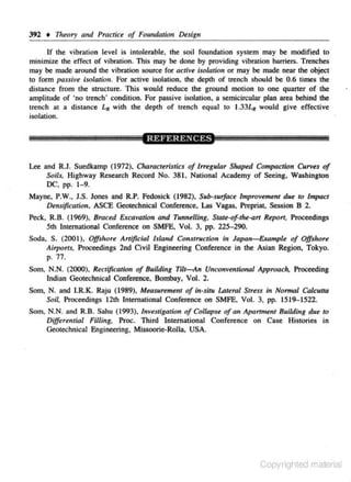
The corresponding stress distribution below the centre. line nnd the edge are shown in
Fig. S.IO. The variation of u,tq with xla and z/a is tabulated in Appendix A.
.
Slllp
width 2b
q
~
q
0.2 M
~
q
0.6
0
1
2
~
I
z
•
I
5
•
/
1.0
1.2
/
lh
3
;;
~
o
.a
I
6
7
8
Fig. $.10 Vertical stress below unlfonn slrlp toad.
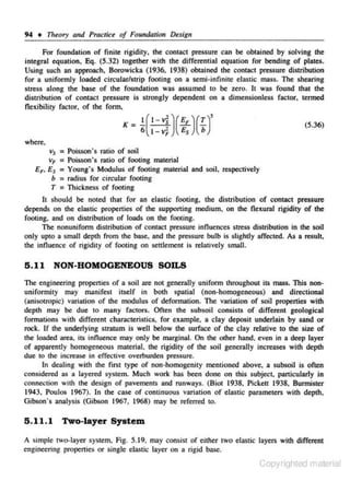
5 .6 .3
TrtBDgUJ.ar Load
The venicaJ stresses in the soil due to a triangular load increasing from zero at the origin to
q per unit area at a dislllnce a [refer Fig. 5. 11 (a)) is given by,
(uJA
or
a.
= !!!..[ran·•(_!_) - tan· •(!.)] - [-q ---"-x-~a]
z
Jra
x- a
x
tr (x _ a)2 + z2
1
-·· = 1l
q
x
a
tan·• (
;; ) -
~
a
_
1
tan·•!.!!.
ax
(S.24)
X -I
t _ __,a'-=--~
a(: -I)'+(J
Copyrighted material

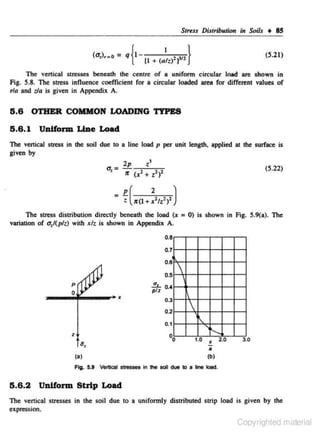
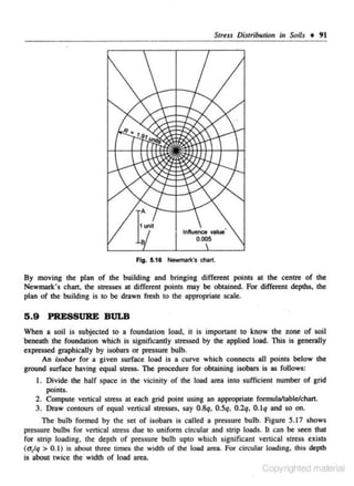
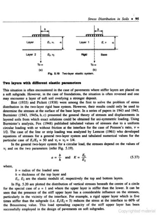
107. Stress Distribution in Soils • 87
For x :;:: a, that is, for points below 8,
'(Jt
-·•)
were 1 = - - - tan-.
h
•
1t
2
a
The variation off with va is shown in Fig. S.ll(b). The tabulated values of G/q for
different values of x/a and va are given in Appendix A.
Zl•
00
•
o.•
0.6
0.5
Stress
/'
q/Unit area
X
B
t
1.5
a,=
qr
2
• A(x, Z)
l
0.2
(b)
(a)
Fig. 5.11 (8) Ver1lca1 stre:M due to • triangular load. (b) Variation of f with ria (stress belOw point 8).
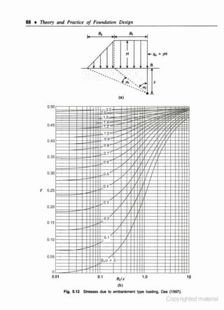
5.6.4 Embankment Type Loading
For an embankment of height H, Fig. 5.12(a), the vertical stress at any poinl below B is
given as, Da.< (1997)
q
l!.p = ; [
81 + 8
B
B, ' (a, + a,) - ~ a., ]
q.
= yH
H
where
(5.25)
= Height of embankment
r = unir weighr of embankment soil
tan·• 81 +
B, - tan·•!!!. rad
l
l
a,=tan -• -B,
-
where I' =
t
l!.p = q.l'
-1'·B.) .
;
(5.26)
f ( a·
The variation of
r
with
~
l
and 82 is shown in Fig. S.J 2.
l
Copyrighted material

108. 88 • Theory and Practie< of Foundation D.sign
8,
I•
•I
(a)
0.50
0.05
0.41l
0.35
n
·n
r
n
0.
"
n
0.01
0.1
S,l z
1.0
10
(b)
Fig. 5.12
s...... ®e 10 embankment type toad>lg, Das (1997).
Copyrighted material

109. Stress Distribution in Soils • 89
5 .7
STRESS AT ANY POINT BELOW RECTANGULAR LOAD
The principle of superposition allows determination of vertical stres:s at any point below a
rectangular looded area. For point A, for example, Fig. 5.13. the loaded area may be: divided
into four s maller rectangles keeping the point A at the comer of each rectangle. The n,
(5.27)
I
•
•
•
II
•
:A
---<)-----------•
.
Ill •
•
IV
Ftg. 5.13 Stresses below point within a toaded rectangular area,.
where q is the applied load intensity and lal' l aw la 1 and larv are the stress influence
11
facrors for points below the comer of respective rectangular areas.
Similarly, for points outside the loaded rectangle. Fig. 5. 14, the vertical stress below
point B may be: obtained as.
(5.28)
II
•
:
'
•
m 9"A :
:rv •
•
·······----- ~ ---··
Fig. 5.14 Stresses belOw I)Otlt outside 1 toa.ded rectangular area.
5 .8
NEWMARK'S CHART
Newmark ( 1942) derived 3 simple graphical c.alculac.ion for determining the vertical stress al
any point within a soil mas.~ for any shape of loaded area.
Let us consider the stress beneath the centre of a loaded circular area. Fig. 5. 1
5.
Copyrighted material

110. 90 • 71Jeory and Practice of Foundation De.Jign
•
/
qtunit
area
z
Fig. 5.15
Stress beneath centre ol a k:laded circular area:
O': = q 1-
{
c:oostructkln of Newmark's chart.
(5 .29)
I .,
}
[I+ (ahtf 2
On rearranging the above equation,
_,,
7· (·-:' )
(5.30)
-1
The interpretation of this equation is that alt. ratio is the relative size of a circular
loaded area in terms of the depth t such that when loaded h gives a unique pressure ratio..
a,lq on the soil at that de pth. By substituting different values of <1,/q in Eq. (5.30),
corresponding values of aft can be obtained. as in Table 5.1.
Table 5.1
Relation~ip
ulz
atq
0.27
0.40
0.52
0.64
0.77
O
.t
0.2
0.3
0.4
o.s
between all and a!q
olz
0.92
atq
1. 11
1.39
1.9t
0.7
.,
0.6
0.8
0.9
t.O
Then, taking an arbitrary value of z (say. 1 em), a series or concentric circles of radius
0.27 em, 0.4 em, and so on can be drawn. The series of rings is further subdivided into a
number of units (say 200) by drawing radial lines from the centre, as shown in Fig. 5.16.
The value of each unit then becomes ( lnOO)q = 0.005q.
To obtain the Stees~ at a point A located at depth z below a footing. the loaded area is
drawn on a tracing paper to a scale z equal to the scale for which the Newmark's chart to be
used has been drawn. The plan on the uacing paper is placed on the Newmark's chart such
that the point A is placed at
he
centre o f the chart. Then. the number of units of the
Newmark 's Chan (N) enclosed within. are counted. The stress at A is given by.
(<TJA
=q
x N x value of each unit
Copyrighted material

111. Stress Distribution in Soils + 91
Flo. 5.1& Newmark's chart.
By moving the plan of the building and bringing different points at the centre of the
Newmark's chan. the stresses at different points may be obtained. For different depths, the
plan of the building is to be drawn fresh to the appropriate scale.
5.9 PRESSURE BULB
When a soil is subjected to a foundation load, it is important to know the zone of soil
beneath the foundation which is significantly stressed by the applied load. This is generttlly
expressed graphically by isobar.; or pressure bulb.
An isobar for a given surface Joad is a curve which connects all points below the
ground surface having equal stress. The procedure for obtaining isobars is as follows:
I. Divide the half space in the vicinity of the load area into sufficient number of grid
points.
2. Compute vertical stress at each grid point using an appropriate formulaltoble/ehart.
3. Dmw contours of equal vertical stresses. say 0.8q, O.Sq, 0.2q, O.l q and so on.
The bulb formed by the set of isobar.; is called a pressure bulb. Figure 5. 17 shows
pressure bulbs for vertical stress due to uniform circular and strip loads. It can be seen that
for strip loading, the depth of pressure bulb upto which significant vertical stress exists
Ca:lq > 0.1) is about three times the width of the load area. For circular loading. this depth
is about twice the width of load area.
Copyrighted material

112. 92
+
17~eory
and Practice of Foundation Desig11
0.05
Strip
COde
wid1h b
dia. b
6 3~--~2~--~
,----~
0~--~,~---±2----~3
rib
Ag. 5.17 Pressure bulb b
circular and s...., footings.
The pressure bulb gives the z.one of soil which influenced by the foundation loading
and is useful in planning soil exploration programmes. and in the study of settlement and
interference of footing.
5 .10 RIGIDITY OF FOOTINGS: CONTACT PRESSURE
Mos1 footings possess a definl!e rigidi<y. 11 is impor1llnl 10 estimalo !be effect of rigidi<y on
the distribution of pressure on the footing base (contact pressure), and on the stress
distribution wi<hin !he soil mass.
According to Boussinesq analysis, the vertical defonnation of a point on the surface of
an elastic half space under the action of a concennted load P is given by
p
2
W=-(1-v)E
trR
(5.31)
For an arbitrary loading area (Fig. 5.13), !be vertical displacernen< of !he point A is given by
(5.32)
where ·F is the loading area over which integration has 10 be done.
Copyrighted material

113. Str~n
Distribution in Soils • 93
With an absolutely rigid foundation, all poiniS on lhe surface of contact will have lhe
s.ame vertical displacement Thus, the condition of absolute ri,g.idity of a foundation is.
v' II
w, = 11<E
p(~ - TJ)d~ dq
F~(x - ~)' + (y -
= const.
(5.33)
TJ)'
The solution of the integral equation for an absolutely rigid circular footing with a
central load gives the contact pressure at lhe point M as:
p(x. y) =
P.
(5.34)
2~[1-((/al'J
where,
a = radius of foundation base
' = distance from lhe centte of base to a given point (( S a)
p. = mean pressure per unit area of the base
'=
It can be seen from Eq. (5.34) !hat for ( = a (i.e. at footing edge). p(x, y) =
0 (i.e. at footing centre), p(x, y) = p.l2.
For a strip footing. the contact pressure at the point M is given by,
p(x. y) =
2p0
;rJ[I - (y/b)2 )
~
and for
(5.35)
where.
y = horizontal distance of lhe point M from tbe eenue of f()()(ing
b = half width of footing
The distribution of contact pressure for an absolutely rigid footing on an elastic half
space will have a saddle like shape wilh infinite pressure at lhe ends, as shown in Fig. 5.18.
However. in actual practice, there is redistribution of stresses over the base (the stresses at the
edge of footing cannot exceed lhe bearing capacity of lhe soil) and lhe contact pressure at lhe
base of a rigid footing tends to become more uniform.
•
Conlact
preS$ure
-
-
Fig. 5.18 Rigid footing: contact pressure.
Copyrighted material

114. 94 + nreory and Practice of Fou11datio11 Desig11
For foundation of finite rigidity, the contact pressure can be obtained by solving the
integral equation, Eq. (5.32) together with the differential equation for bending of plates.
Using such an approach, Borowicka (1936, 1938) obtained the contact pressure distribution
for a uniformly loaded circular/strip footing on a semi-infinite e lastic mass. The shearing
stress along the base of the foundation was assumed to be zero. It was found that the
distribution or contact pressure is strongly dependent on a dimensionless factor, termed
flexibility factor. of the fonn,
K=
~(: =j,)({;)(f)'
(5.36)
where-,
v5 =Poisson's ratio of soil
vF = Poisson's ratio of footing material
EF. Es = Young's Modulus of footing material and soil, respectively
b = radius for circular footing
T = Thickness of footing
It s hould be noted that for an elastic footing. the distribution of contact pressure
depends on the elastic properties of the supporting medium, on the flexural rigidity of the
footing, and on distribution of loads on the footing.
The nonunifonn dislribution of contact pressure influences stress distribution in the soil
only upto a small depth from the base. and the pressure bulb is slightly affected. As a. resu l~
the innuence of rigidity of footing on settlement is relatively smaJJ.
5.11
NON-HOMOGENEOUS SOILS
The engineering propenies or a soil are not generally unifonn throughout its mass. This nonuniformity may manifest itselF in both spatial (non-homogeneous) and directional
(anisotropic) variation of the modulus of deformation. The variation of soil properties with
depth may be due to many factors. Often the subsoil consists of different geological
formations with different characteristics. for example. a clay deposit underlain by sand or
rock. If the underlying stratum is well below the surface of the clay re lative to the s ize of
the looded area, its influence may only be marginal. On the Other hand. even in a deep layer
of apparently homogeneous material, the rigidity of the soil generally increases with depth
due to the increase in effective overburden pressure.
ln dealing with the first type of non-homogenity mentioned above. a subsoil is often
considered as a layered system. Much work has been done on this subjecl, particularly in
conn~tion with the design of pavements and runways. (Biot 1938. Pickett 1938, Bunniscer
1943, Poulos 1967). In the case of continuous variation of elastic parameters with depth.
Gibson's analysis (Gibson 1967. 1968) may be referred to.
5.11.1 Two-layer System
A s imple cwo-Jayer system. Fig. 5.19, may consist of either two elastic layers with different
engineering propenies or single elastic layer on a rigid base.
Copyrighted material

115. Streu Dutrfbutlon In Seils • 95
b
E, v
t
To •
To•
(I)
~
-
(b)
'IW<Ho)'Of olostic oya-.
Fig. S
.1t
This situation is on.:n encounlered in the case or pavements when: stirrer layers are placed on
a soft aubpade. However. in the cue of foundations, the situation Is on.:n rcvened and one
may encounter a layer of soft soil overlying a llrOQger clepooiL
Blot ( 1935) and Picken ( 1938) were among the fust to solve the problem of..,....
dillribution in the two-layer ri&id bose syown. However. their rcaults could only be used to
ddetmine the ~tresses at the surface of the bose layer. In a series of papen in 1943 and 1945,
Bunnister (1943. J945a. b. c) presented the geocnl theory of ~tresses and displacements in
layetcd soils from which exact solutions could be obtained for axl·aymmeuie loading. Using
Bunniltet's analysis, Fox (1948) published tabulated values of sueues clue 10 a uniform
circular loading wilh or wilhout friction at the inletface for the cue of Poisson's ratio, v =
112. The case of the line or strip loading was analyzed by Lemc:oe (1961) who developed
equations of stre&..a for a general two-layer system and ubulated numerical values for the
particular case of £ 11£2 • SO and v 1 = v, = 1/4.
In the general two-layer syatem for a circular load, the SII'C&Iel depend on the valuea of
v 1 and on the two pllamtten (refer Fig. 5.19).
Q
b
=- and K- .§_
h
-e.
(5.37)
where.
b • radius of the loaded area
lo s lhieknal of the top layer and
£ 1•
~
are the elastic modulii or. respectively the 1op and bOI2om layers.
In Ag. 5.20 are plotted the distribution of vertical streue1 benealh the ceniJC of a circle
for the special cue of a • I and where the upper layer is stiffer lhan the lower. It can be
seen that the presence of lhe •tirr upper layer has a considerable innuence on the stresses.
particulatly In the vicinity of the interface. For eumpk. a rigid upper layer which is five
times stirrer lhan lho aubgrade (i.e. £ 11~ = 5) tcduces lhe all'Css at the interface 10 60% of
the Bou•sincsq value. This load spreading capacity of the Iliff upper Ioyer has been
successfully employed In the de•ign of pavements on sort subgrades.
l OiJyrighted ma.enal

116. 96 • 17oeory and Practice of Foundation !Hsign
1
v, •0.2
"'J a
z
o.•
b
"'l a 0 .•
3
0
(a)
2
b
1i
3
•
5
(b)
Fig. 5.20 T- . loyer aysan: Etlect of rlgidl1y ol upper l~r on the vettical
tnss btne8lh centre of a uniform drcullr toed (after Boonisler 1963).
The effect of relative size of loaded areas and thickness of the upper layer on the
vertical stresses at the interface is shown in Fig. S.19b. The upper layer is most effective in
spreading the load when its thickness lies between b and 3b while for very thin and very
thick layers, they approach the Boussinesq values.
The case of a foundation where a sofllayer i's unde..Wn by a stiffer deposit (£1/£2 < I)
has not been evaluated but from exb'apolation. it can be concluded that the stresses in the
upper layer will, if anything, be greater than those for a homogeneous medium.
&mcle e!eotte la:rer oa a
J'l&ld -
This is a special case of the above problem with the elastic modulus of the bouom layer
E2 = "'· The problem was first solved by Burmister ( 1956) who extended his earlier work to
analyze the stresses and sb'ains in the upper layer of a two-layer rigid base system. From his
influence charts, it is possible to obtain che complete pattern of stresses and displacements
under the comer of a uniformly loaded rectangle for Poisson' s ratio, v = 0.2 and 0.4.
The same problem was considered in detail by Poulos (1967), who used Burmister's
theory to compute a set of influence factors for stresses and surface displacements due to a
point load. for values of Poisson's ratio, v = 0, 0.2, 0 .4, and 0.5. By integration of these
point load factors, he then calculated the corresponding influence factors for different loading
types.
The vertical and radial streSSes beneath tbe centrt:. of a loaded circle for values of
hlb = 1, 2, 4. and 8 and v = 112 are shown in Fig. S.21. The stresses for the homogeneous
hal.f·space (Boussinesq) are also piOited for comparison. It can be seen that the presence of a
rigid layer at a shallow depth relative to the size of the loaded area significantly alters the
stress pattern. For small values of hlb just undemellth the load, vertical stresses may even be
greater than the applied pressure. However, with increasing depth, the effect of the rigid base
Copyrighted material

117. Stress Distribution in Soil.' + 97
gradually diminishes and for hlb > 8, the stresses are almost indistinguishable from the
Boussinesq values.
Oia2b
q, !
q
.ll I I I J o.2 o.•
0
.... ·--
~ 'i
·,A
3
z
b
1.2
1.0
. 1
,2
2
0.8
' · · ;1;1 ~1.0
.
~
....
~
1
q
0.6
~-•
.I
v.
..... b ~
'
'I j
•
.c
.8
5'
z
-
8
a,,lWo-layer rtgld base
. .. ..... CJ,
(Met Poulos 1987)
v. 0.5
1
.
8
Fig. 5.21
~
---- BouNinasq
Figures on curves are values of hlb
I
I
olslreaaeo In -.layer rigid basa syolem (after Poulos.
11187~
5.11.2 Three-layer s,-.tema
The analyses of three-layer soil syslemS (Fig. 5.22) are much more complex than for lwolaye.. and solutions have only been obtained for stresses and deflections beneath a uniform
circular load. Burmister (1945) was lhe lil$1 10 develop the general theory for such a system
with both rough and smooth interfaces.
Cia 2b
q
"'4.P ~
layer 1
E~o
Layer 2
E,. ,
Layer 3
.qu
a~
h,
a,,
Tow
~ig.
,.,
w(O.O)
Es. ''l
v,
k1
•
E1!~
k2 • EiEs
• = blh,
H • h11hoz
5.22 Th,.....ayet elaStic system.
Copyrighted material

118. 98
nttory and Proctict of Fou11dorion Design
t
Burmistcr's equations were used by Acum and Fox. (1951) to calcuhue lhe stresses at
the interfaces (for v1 = v2 = 0.5 and for fu ll continuity between the layers). Schiffman
(1957) presented methods for numerical solutions of influence values and tabulated resulrs for
a particular case. In later years. Bunnister's work wa..~ extended to compute the stresses and
deflections for any combination of thicknesses of the individual layers and size of the loaded
area. Jones (1962), Peattie (1962), and Kirk ( 1966) have published chans and table.• giving
the stress fac tors for any combination of three-layer systems while De Barros ( 1966) and
Uyeshita and Meyerhof ( 1967) have published those for deflection factors.
The stress and strains in a three-layer medium are governed by the following
dimensionless paramelers:
b
h,
E
a= - ; H = - ; k1 =
(5.38)
and k 2 =
h,
E: ;
h,
where.
b is radius of the loaded circle
h 1 and h1 are thicknesses resptctivcly of the firs1 and second layers (The bottom
layer is semi ~ infi nite).
£ 1• £2• and £ 3 are the elastic modulii of the JM, 2"', and the 3,. layers respectively.
Figure 5.23 shows the effect of the relative thicknesses of the two stiffer upper layers
on the stresses and deflections beneath the centre of a loaded circular area. for the particular
case of h 1 + h'2 == 2b. For 1hc purpose of comparison. the Bous.sincsq stresses and the
deflections calculated on the basis of Boussinesq stress distribution are also plotted. It can be
seen that the actual values are lower than those given by Boussinesq although the maximum
discrepancy in deflection is not more than 25%.
1.2
1.0
...
0.8
tFIo-
0.6
.;:~
•
q
-- --
h,+h, •2b·
v,
- -.-
"1 c II) ;r;
;r;
' ~ '-.
''
o.•
=- 0.2
--
--
w (ll, 0)
1'-t.
_: ' ~-
1?l.r
0.5
a ~·
~
h,
Oia2b
-l- H
fH
W(O, 0)
E, =
a.,
4&
Ez. 2E)
a,, .I
r9
k,. 2
k2. 2
' ,,
- - - Rigorous solu1ion
.... • • • • • · Boussinesq
0.2
0.4
0.6
,.,
0.8
1.0
_!L
Fig. 5.23
I
)
I
l
Stress and displacemen1 In three-layer system (efter Jones 1962. Uyeshlla
and Meyo<hol 1967).
Copyrighted material

119. Stress Distribution in Soils • 99
For the situation where the layers become successivley stiffer with depth (l 1 :: 0.2,
l 1 = 0.2), the assumption of homogeneity will underestimate the slresseS by up to 30% for
h 1/h 1 + h 2 ~ 1 while for smaller relative thicknesses of the top layer, the enor is
considerably less, as illustrated in Fig. 5.24.
'·2
I .0
.;:~
..
..
.
~
....
0.8
o.2
,
.., • ,, • ' • 0.5
~
0
0
:- ..
J
0.2
-- -- "'
--
0.4 "' 0.6
0.8
w
-1-H
CTzt., ~ E
:
I
:a ,:-.,
''
--
Oia2b
•• "a~
~ >rlru.t,
0.6
0.4
q
h,+hz•2b
+ 5£
25E
k , • 0.2
k2 • 0.2
' .0
-Rlgorou·--- - 8 -
"'+">
F~.
5 . 11.3
5.24 Stress In a lh,...tayer system (after Jones 1962).
Multilayer Systems
The problem of multilayer system involves immense complexjty and to dace no analytical
solution is available for anything consisting of more than three layers. Vesic (1963) has
5uggestcd an approximate method of c:alc:ulating the elastic settlement of a foundation on a
multilayered medium assuming Boussinesq stress distribution but using the proper elastic
modulus for the respective layers. His chans and method of calculation are shown in Fig. 5.25.
-·-·
•
<
Oia 2b
- w
w ...,._ ,
La~r
z
;;
n
...
Settlement due to
dW,. = W ,o
la)'tf' n
1 - ,.
Wn • 1
= 2qb"""'E,;'"""(/,.- 1n .. 1) =
4/
2qb~
Totll-
w0 =wn=2qb~
"·
. I
Gopyngnteo n atena
Fig. 5.25 Approximate method of calculating set1tement In miAiilayer elastic syseemt (after Yeti<: 1963

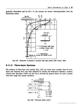
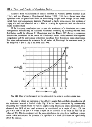
120. 100 + Thtory and Practice of FoundaJ;o, Dl!sign
Vesic observed that in three-layered systems, the shape of the deHected surface computed by
this approximate technique agrees better with measured deflections of pavements than the more
rigorous analyses.
De Barros ( 1966) proposed an approximate method of reducing a multilayer system to
a three-layer one. keeping the subgrade unaltered, by successively attributing to the two
adjacent layers an 'equivalent mcxlulus' according to the equation
(5.39)
He found that using this technique and reducing a lhree-laycr system to an equivalent
two-layer one, the approximate method is correct to within 10% for lr21b > I and 14% fo~
h, tb > 2 .
An analogous expression was first proposed by Palmer and Barber ( 1940) to reduce a
two-layer system to an equivalent homogeneous medium which yielded deflections very close
to Burmister's two-laye- analysis.
r
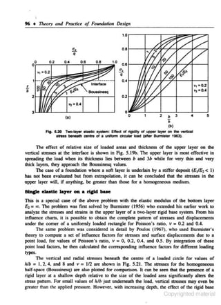
5 .11.4 Non-homogeneous Medlum
The problem of lhe non-homogeneous soil medium whose modulus of elasticity varie.~ as a
continuous function of depth has received only IH:nited attention so far. Korenev (1957).
Sherman (1959), Golecki (1959). Hruban (1959). and Lekhnitskii (1962) have studied
particular problems of non-homogeneity. but no comprehensive
~eory
had been presented
until Gibson developed the theory (Gibson 1967. 196&) of stresse.• and displacements in a
non-homogeneous. isotropic elastic haJf.space subjected to strip or axially symmetric loading
normal to its place boundary, Fig. 5.26.
_jq~·!]·!]f!]·~r~~'!:'!ai..._. •
I
i
I
I
I
A
G{l) = G{O) + mz
~ = G(O)
m
••
'
''
l
..
G{z) • G{O) G{z) • mz
jj•oo
fJ= 0
Fig. 5-26 ~· elastic medium { - Glbooo 1967, 1968).
A semi-infinite incompressible medium whose mcxlulus of e lasticity increases with
depth from zero at the surfa.:e (i.e. p = 0), behaves as a Winkler spring model. In other
words , the surface settlement of a. uniformly loaded area on such a medium is direclly
proportional to the applied pressure and iodependent of the dimensions of the load.
Copyrighted material

121. Str~ss
Di.ttribution
i11
Soils + 101
The distribution of stresses in a semi-infinite medium is not significantly affected by
this type of non-homogeneity. Figure 5.27 shows the streSS distribution for {Ji b = 0.1 and 10.
Indeed. the two limiting cases {Ji b = 0 and {Ji b = "' give exac:dy the same stresses while in
the intermediate range 0 < f31b < co, both the ven ical and horizontal stresses te nd to be a
little higher than the corres ponding stresses for the homogeneous medium. though the
difference is never greater than 10%. However, over most of the range (0 < /Jib < 0.5 and
S < fJI b < co). the discrepancy is less than 5%. This observation is true of ven ical and
horizontal stresses due to both axi-symmetric and strip loadings, as depicted in Fig. 5.28.
!!L a,.
q. q
. 1h 2b
s._, Clrde
dia 2b
0.2 0.4
..-;,
2
.(,;.
,,
/
/
I
f
f
3
I
1.0
-~
<
0
1
o.e
0.6
I
I
4
'
,
'
-• _ _ Sir? BouS$1nesq
Clrde,
_
I
° Citde 'ftlb
• Strip
I
5
= 0.1
I
8
I
1
I
I
8
f'u.
5.27 Vertical e.trass benealh centre of foundations: non-homogeneous medium (Som 1968).
(al Circle dla 2b
1.0
1.0
(b)
Sir?
width
•
•
•
•
•
•
•
•
•
•
•
0.8
0.8
1
0.8
0.6
!!..
q
2
0.4
0.4
•b
l
0.2
0.2
•
•
•
•
•
•
0
4
8
fllb
1 8
1 4
.,.
(ftlb)
.
•
2b
![
1
•
•
•
•
•
•
•
•
2
•
•
•
•
zl
4
8 181 4
fllb
. ,.
(~/b)
0
I . I
vOfJytlgn.co ma ena
Fff!J. 5.28 Effed of noo-homogenei ty on the vertical stresses beneath centre of foundation&.(Som 1968).

122. 102 • Theory and Practice of Foundation Design
Ex<ensive field measurements of stresses reponed by Plant<ma (1953). Turnbull et al.
(196 1), and the Waterways Experimental Station ( 1953, 1954) have shown very close
agreement with the predictions based on Bous.sinesq analysis even though the soil media
varied from non-homogeneous deposits (Plantema) to fairly homogeneous test sections of
clayey silt and sand (Turnbull et al.). This is cenainly in agreement with the theoretical
re.<ults presented here.
If the foregoing conclusions are correct, the settlement of a foundation on a nonhomogeneous medium may be calculated reasonably accurately by assuming that the stress
dislribution could be obtained by Boussinesq analysis. Figure 5.29 shows a comparison
between the settlements of the centre of a uniformly loaded circle obtained from rigorous
computation and the approximate settlements calculated from Boussinesq stress distribution.
11c latter underestimates the settlement ror all values of {jib 1hough the max..imum enor (in
the range 0.5 < {Jib < 1.5) is no more than 10%.
0.5
100
l
o.•
.I
/J
,
O.J
/..'
./ ,
qb
w(O,O)/ G(O)
0.2
/.
,,
0.1
I"
0
0
Fig. 5..21 Effect of
r-'
o.•
-0
--
~
80
60
..!!..%
wo
/
•o
•
2(1
o 1.0
.s
o.&
1
fllb -->!<--- (Ptbl
non~lty
I
0
o.2 o
on the setiJement of lhe centre of a uniform dra.llar load.
In orde,r to obtain an indication of the effective depth that contribu1es towards most of
the settlement beneath a loaded circle. Fig. 5.30 has been constructed by successively
integmting the venical strains for various depths using Bous.sinesq stress distribution. It is
observed that 80% of the total settlement is contributed by a depth of only 1.5b for
{Jib = 0.1 and 5b for {Jib = ao while a depth of Sb accounts for as much as 90% for all
values of {Jib. This is consistent with the st:n:ss-dislribution in a two-layer Jjgid base system.
where, it has been s hown, the presence of a rigid layer at a depth of Sb does not significantly
o.ff~t the s1resses.
Copyrighted material

123. Stress Distribution in Soils + 103
Cia 2b
z
b
0
2
1
3
•
5
6
7
6
9
10
Oe(>UI (Zib)
Fig. S.30 Ef'fec:ltve depth ol soil beneath a circular foundadon: non-homogeneous medil.m.
5 . 12 NONLINEAR SOIL
The problem of s1ress analysis in a soil medium with a nonlinear stresS-stroin relationship is
immensely complex and no general solution is available yet. Huang (1968) presented a
method of analyzing stresses and displacements beneath a circular load in a nonlinear soil
medium whose modulus of elasticity is a function of the stresses.
·
E
= Eo (I
+ c6 (u, + u, + u 8 + c 7 yjb)J
(5.40)
where CJJ (the nonlinear coefficient) and c1 (the body force coefficient) are material
parameters. He divided the semi·infinite medium into a multilayer system assuming a rigid
base at a depth of IOOb (see Fig. 5.28) and assigned to each layer, a modulus corresponding
to the stres.ses at the midpOint. Employing Burmister's boundary and continuity conditions
(Bunnister 1943. 1945} and using the method of successive approximationS. Huang c.a lculated
tbe stresses and displacements until two consecutive iterations gave thd &arne modulus. His
results are shown in Fig. 5.31. Again a close agreement with the Boussinesq stres.s
distribution in noted. Comparison between the actual settlements calculated rigorously by
Huang and the approximate settlements calculated on the basis of Bous.sinesq stress
distribution but using the proper variation of E with depth show that the two methods do not
differ by more than 10%. as shown in Fig. 5.32.
However. the assumption made by Huang. that each layer has uniform modulus means
that the problem is, in effect, reduced to a multilayer Burmister problem with the elastic
modulii detennined by the stresses in the centre of the individual layers as shown in
Fig. 5.32.
Copyrighted material

124. 104 • 111eory curd Proctice of Foundation Des1'gn
q
Ilia 2b
0.2
o.•
0.6 q
1.0
0 .8
0
./
1
/Y. r-- ,-s
2
1
'f
/
~ c1
3
z
b
1
= o (BousslneSQ}
q..wi•2b
•
E,
...
c
E,
8
5
E•E0 (1• c(al • o,. • a, + cl'rltb)J
8
E.
"'
<>
E.
c, . 0.02
...
..
E.
c
7
N
E,
"
- :a
...
!
i
E J RKikl
8
Stresses in nonlnear soil medi001 (after Huang 1968).
Ftg,. 5.31
E
0
1.8
r
~
qb
w(O,O)/ Eo
1
0
2
c,
3
•
0
•
b
8
8
5
10
- - Rigorous computation
~•
• • From BousSineSQ stret.$ distribu6on
100
Fig. 5.32
•5
'
''
'
'
z
0.2
2 3
2
0.8
r:.::- -----
1
'
1.2
~--....;
0
6
7
8
!
•
•
•
i
'' i
' !E: E0 (1 • c1(a,. •
' • .,., + c,rtlb))
'' i
' !
'
' '
'
'' i''
' !
'
' '
'' ;'
' '
'
' '
"'
- - c, = 1
----- c, • 3
-- · ~
.. c, = 5
c, • 0.02
''
''
'
'
•
'
Setuement at centre of circular load: nonllneat mec:lit.m.
Copyrighted material

125. Strtn Distriburio" in Soil.f
+ 105
At present. the problem of nonlinear soil medium is best solved by numerical melhods
using computers. Finite element modelling is most widely used (Zicnkiwicz 1971). However,
a detailed treatment of the finite clement analysis is beyond lhe scope of this book. The
reader may refer to the relevant liternture for furlher details (Desai and Abel 1972. Desai and
Christian 1977, Smith 1988).
The distribution of venical and horizontal stresses wilh depth, along the centn: line of a
model c::ircular footing resting on a saturated normally consolidated clay. with a load
intensity, qtu:~ = 0.35, 0.77, and 1.05 (q = applied pressure, u;. = effective vertical
consolidation pressure). as obtained from a nonlinear finite element analysis ((Das 1975) and
(Das and Gangopadhyay 1978)). is shown in Fig. 5.33. On the same figure are plotted the
stresses. obtained from clastic analysis and lhose obtained by measurement at qla'w, ;; I.
using pressure cells. It can be !;Ceo that vertical stresses do not change mucb with load
incrementS and elastic theory c,an predict the stresses quite well but horizontal stresses are
significantly dependent on load increment. When the loading is smaJI (qlu~ = 0 ..35 in this
case), the elastic theory may be capable of predicting horiront~l stn:sses but at higher loads,
non·linear analysis is necessary to predict horizontal stresses satisfactorily.
Normalized stress !?t.~
q' q
02
0
04
.
06
~
l.k'-
1
I
2
/.;
v/ v
.
•
10
08
1-'-
~
12
:?
~
l
I
Legend
I
Firite element !.&. ~
••
••
Non linear ll.
Measun>d
6
I
7
0
cr. • Hortzontal stress
cry a Vertical stress
q = Footing presswe
y • 001)111 belOw foot>1g
b • Footing radius
8
Fig. 5.33 Compalfson ol ,,...... obtained from linea< and no<Hinear analySis (Das 1975).
Copyrighted material

126. 106 • Tl1eory and Practice of Foundation Design
Therefore, it appears that any deviation from the classical problem of homogeneous
nonlinearity of stress-strain relationship or in terms of nonelasticity. eilher in terms
homoge,neity of 1he medium will only have a marginal effect on the stress distribution so
long as the medium is subjecled to certain boundary stresses. The displacements will, of
or
course, be significancly affecc buc from !he foregoing ic can be deduced c !he seulemenl
ed
hac
can be obtained with reasonable accuracy, by assuming lhe Boussinesq stress-distribution but
c
oking accounc of the proper scress-strain relationship and/or non-homogeneity in calculating
the scrains. Also, as long as che pressure bulb due co a footing load is reslricted wilhin !he
upper layer of a soil deposic, the Boussinesq analysis should be reasonably valid,
notwithsc
anding any non-homogeneity below chac layer.
5.13 APPROXIMATE METHOD OF DETERMINING VERTICAL
STRESS
The pressure on footing founded at or near the ground s urface gets dispersed to a wider area
at a depth. In !he approximate melhnd, !he scress dispersion is assumed along lines through
the edge of !he footing 01 an angle ex = 26.5°, that is, 01 a slope of 2 horizontal co I vertical,
as shown in Fig. 5.34.
Q
r;·
l
..
2~
..
•
1'
lri~~Hiiiiiil~~;hq,
Fig. 5.34 2:1 dispersion method for dlsmbution of vertical stress due to surface toad.
Accordingly at any depth
z.
the venical
u. =
•
s ires.~
is given by.
qLB
(8 + z)(L + z)
(5.41)
The stres:.~ thus calculated will be unifonn over the dispersed area. However, in actual
practice. the s tress wiJI be more towards the centre and Jess towards the edges as shown by
broken line in Fig. 5.34. The approximate method is not generally recommended for detailed
design. although the method comes handy for rough calculations in the absence of necessary
charts and tables.
Copyrighted material

127. Stress Distribuliotr in Soils + 107
Example 5.1
Figure 5.35 shows four vertical loads of I000 leN each placed at the comers of a square of
side 5 m. Detennine the increase or venical stress 5 m below
(a) each load
(h) midpoint between adjacent loads
(c) the centre of the rectllngle
Sm
0, "1-- - -0,
:::-1"
Ftg. 5.35
Solution
From Fig S.4. vertical stresses due to a point load
u, = ~ 11 ,
••
Point A
where /8 = / (rlz)
Q1 = 1000 kN; rlz = 0; 18 = 0.478
5
Q2 = Q. = 1000 leN, r/z = 5 = 1.0; /8 = 0.084
Q3 =
J<52 ... 52)
= 7.07 m;
(UjA
~ z 7 ·~
= 1.41; '• = 0.031
100
= -52 [0.478+2(0.084)+0.03 1J =27.1JcN/m2
Point 8
r
2.5
Q, = Q, = 1000 leN; - = z 5 = 0.5; '· = 0.27
r
Q3 = Q. = 1000 kN; -
z
J5· ... 2.52
=
5
(u,)s =
100
5'
= 26.6
= 1.12; '•
= 0.062
[2(0.27) ... 2(0.062)1
lcN/m2
Copyrighted material

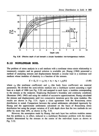
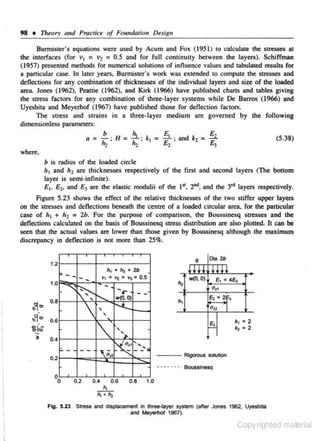
128. 108 • 11reory and Practice of Foundatiolf Du,.gn
Point C
Qt
=Q, =Q) = Q, = 1000 kN
~r2.--=5,:-+ 2.52
--.,-
r
= -'-----,5: - - - =o.71: 1, = 0.11
1000
(<>,lc = __,- [4 x 0.17)
:.
s
= 27.2 kNim'
Example 5.2
Figure 5.36 shows the plan or a nexible rafl fou nded on lhe ground surface. The area
suppOrts a uniform vertical load or 200 kN/m 2. Estimate the increase in vertical stress 15 m
below point A.
,.
30m
15m
"!"
T
.,
15m
l__
A
Fig. 5.31
Sol uJion
Consider <WO rectangles (I + II) and II wilh lhe point A at lhe comer of each rectangle.
(UJA
=q l -; lau)
(lat•l
Rectangle (I + II): 15 m x 45 m
nr
=
45
"i5
15
= 3.0; n = 15
= 1.0,
= 0.201
/•t•n
Rectangle II: 15m x 15m
m=n=
(u,}A
IS
15
= 1.0; /
0
u
= 200 [0.20 1
= 0.174
I
2
X
0.174]
= 22.8 kN/m2
Copyrighted material

129. Strt.JS Distribution in Soils • lt9
Example 5.3
Figure 5.37 shows a raft foundation (10m x 20m) built 5 m from a tower. Detennine the
increase of stress 5, 10, 15, and 25m below the tower and draw the stress distribution. (Take
q. = 100 kN/m 2)
I•
•1•5m•l
20m
•oi [--------'--------r_:~;J~.w"
(<1J. I<Nirn'
0
5
10
_
,..s,
.o_-
5
96
15 F ·==----l
g 10r
!
25 7••
Fig. 5.37
Solution
Consider rectangles 0 • II) and U with point A below each rectangle.
Recungle (I • Il): 25 m x 5 m
Rectangle II: 5 m x 5 m
Influence f!!.ctor
Depth (m)
5 m
"
10 m
n
15 m
"
25 m
n
'·
s
0.204
I
Example 5.4
kN/m2
Ia u
+ II
2.5
0.5
1.67
0.33
1.0
0.2
1.,.) (<1,). = 1001.,
Ia = 2(/oi + IJ
0.136
0.094
0.054
1.0
1.0
0.5
0.5
0.33
0.33
0.2
0.2
0.174
0.06
6.0
0.096
0.08
8.0
0.046
0.096
9.6
0.017
0.074
7.4
.
Figure 5.38 shows the section of an eanh dam. Determine the increase in venical stress 3 m
below points A and B.
Copyrighted material

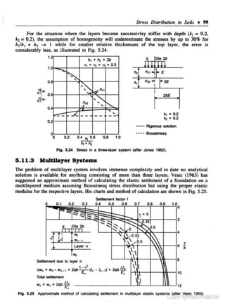
130. 110
Theory and Practice of Foundation Design
t
6m
6m
6m
q
- ,_
3m
'''
'''
'
/('((~
3m
r
p
__
I
3m ._
- '-· B ·-
''
''
''
'
'~
u
s
,.,
Fig. 5.38
$elution
Point A
Stress due to s
trip load qmt:
2a = 6m
z=3 m
q = 50 k.N/ m 2
a,
= q(l.,) where Ia =I ( ~ , ; ) . from
X
l
Here. -
= 0; -
a
a
3
= -
3
Eq. (5.23)
= 1.0: Ia = 0.96
Stress due lo triangular load, pqr
= 6m
a
z=3 m
q = 50kN/m2
<1.
•
=qUa> where Ia
Here,
X
9
=I(!.~).
a a
l
from Eq. (5.24)
3
- - - - 1.• - - - - 0 5· I q -0 06
5·
- ·
-· ·
a
6
a
6
(a.). = 50[0.96 + 2(0.06)]
=54 kN/m2
Point B
Stress due to strip load: qurt
X
-;; =
9
3
= 3.0;
l
0
= 1.0; Ia = 0.003
StreSS due to trinngulnr load: pqt
X
a
= 0;
l
a =
3
6
= 0 .5: 10 = 0. 13
Copyrighted material

131. Str~ss
Distribution in Soils • I 11
Stress due to triangular load: rus
= 3: -l = 0.5: 1, = 0.002
a
(a,)8
= 50(0.003 + 0.13 + 0 .002)
= 6.75
kNJm2
Example S.S
Figure 5.39 shows a 20m dia x 15 m high ste<:l storage mnk founded on RCC raft (SOO mm
thick) 5 m below GL Determine the increase in vertical stress along the cenue of the tank
10m. 20m and 30m below the foundation when the tank is filled of water. Draw the
distribution of vertical stress increase with depth and superimpose the same on the in·situ
suesses to obcain the variation of stress increment ratio llptp0 with depth. Take unit weight
of soil = 18 lcN/m3.
20m
I·
10m
5m
t.piPo
---,--.-T
Ol
!
E
i
0.~· ·
0
Po+ AP
10J
'
!
!
.•
I
a 20~'
'
•
.'.
.
'
''
'
''
t.O
'
'
''
''
•
''
'•
i
I
1
30-i- - - - - ' ·L-..J
Fig. 5.39
Soluti<Jn
Water load = I S x 10 = 150 kN/m2
Self weight of foundation = O.S X 24 = 121cN/m2
= ISO + 12 = 162 kN/m2
Pressure reduced by excavation = 18 x S = 90 lcN/m2
q..,. = 162 - 90 = 72 kN/m2
q,..,
Copyrighted material

132. 112 • Theory and Practice of Foundation
Depth (m)
0
10
20
r
~
a
a
0
0
30
0
0
40
0
D~~·ign
tJp = q00 I a (kN/m 2) p 0 (kN/m2)
lq
0
1.0
1.0
2.0
0.65
0.28
3.0
4.0
0.13
0.08
90
72.0
46.8
180
20.2
360
540
720
9.4
5.8
llp
<0.8
0.26
0.06
0 .17
0.008
Example 5.6
A reinforced concrete tower is provided on a ring foundation of inner diameter 6 m and
outer diameter 12m, as shown in Fig. 5.40. If the foundation carries a distributed load of
150 kN/m2, de.termine the vertical Slte$S distribution at a depth of 6 m below lhe foundation.
Use Newmark's chan.
/~
I
I
'
I
:
I
I
I
I
I
I
'
I
I
I
I
II
·
I
I
I
~
l?@ml
i
IB !A
~ en
c
I
•
I
~
II
•
I
•
12 m
Fig. 5.40
Solution
Draw the plan of !he foundation to scale, 3m = lhc seale of the Newmark's chan to be used,
as in Fig. 5 .41. Then place poiniS A. B. and C successively at the centre of the Newmark's
cha.n and count the number of units enclosed in CD4il case. Then,
0: :
Vertical Slte$S below
11(0.005)
X
q.
A = 70 x 0.005 x 150 = 52.5 kN/ m 2
B = 60 x 0.005 x 150 = 45.0 kN/m2
C = 46
X
0.005
X
150 = 44.5 kN/m2
Copyrighted material

133. Stress D,.striburion in Soils + 113
Fig. 5.41
Example 5.7
Solve Example 5.2 by Newmarlc's chart.
Sofuh·on
Draw the plan of the raft on uacing paper to a scale, 15 m = scale of the Newmark's chart,
Fig. 5.41. Place point A at the centre of the Newmark's chart and count the number of unitS
enclosed by the diagram. Then,
(CTJA
= 23.5 X 0.005
= 23.5 kN/ m2
X 200
Ahlvin. R.G. and H.H. Ulery (1962), TabulaJed Values for Det<nnining the Complete
Paltun of Str~.nes, $/rains. and DejUcrions Beneath a Unifom• Circular Load on a
Homogeneous Half Space, Highway Research Board Bulletin No. 342, p. I.
Biot. M.A. (1935). The Effect of Certain Discollfinui/ies
Loaded Soil. Physics. Vol. 6. No. 12, p. 367.
011
the Pressure Distribution in a
Bishop, A.W. (1952), The Stability of Earth Dams, Ph.D. Thesis, University of London.
Copyrighted material

134. 114 + Tl1e0ry n11d Practict of Fowulation D~sigu
Borowicka. H. (1936), lnjlutmce of Rigidity of Circular Foundutlo" Slab on th~ Distribution
of Pressures over the Contact S11rj'ace. Proc 1st Int. Conr. on S M & F E. Vol 2,
pp. 144-149.
n.~ Di.ttributiou of Pr~SSIIr~
tmdu a Unifonnty Loaded EJa.ttic Strip
Resti11g o, Elastic·isotrope Ground. Zued Int. Conf. on Bridge & Str. Engs, Beriin.
Borowicka. H. ( 1938).
Boussinesq. J. (1985), Applicatio~r d~s Poremial a L · Etrtdt de L · equilibre et tu Movement
dt.f So/ides Elas tiques. Gaurhiers Villars, Paris.
Brooker, E.W. and H.O. Ireland ( 1965), Earth Pressure at Rest Related to Stress History,
Cmwdimr Geoteclmical Jo11mal. Vol. 2, No. I, Feb. 1965.
Burmistcr. D.M. (1943). Tlteory of Str~nes and Displactmtmts in lAyertd Systems, Proc.
Highway Research Board, Vol. 22. pp. 127- 148.
Burmister, D.M. (1945 a). The General Theory of Stresses and Displacements in Layered
Systems. Joumal of Applied Plrysics, Vol. 16. No. 2. pp. 89-96.
Burmister. D.M. (1945 b). The General Theory of Stresses and Displacements in Layered
Systems. Joumol of Applied Physics. Vol. 16, No. 3. pp. 126-127.
Burmistcr. D.M. (1945 c). The General Theory of Stresses and Displacements in Layered
Systems. Joumal of Applied Plrysics, Vol. 16. No. 5, pp. 296-302.
Carothers. S.D. ( 1920), Plane Strm'n: Direct Detenm"
uatio" of Stresses. Proc . Royal Society
Scrie.< A: Vol. 97, pp. 110-123.
Das. B. (1997). Ad••anced Soil Mechanics. 2nd ed., Taylor and Francis, Washington, D.C.
De Barros. S.T. (1966), Deflection Factor Charts for Two and 17tree lAyer Sysums,
Highway Research Record No. 145, p. 83.
Desai. C.S. and J.F. Abel (1972). lmroduction 10 Fiuilt! Element Mttlrods, Van Nostrand
Reinhold, New York.
Desai, C.S. and J.T. Christian ( 1977). Numerical
McGraw-Hill. New York.
M~tlrods
in Geotttclrnical £11gineeri~rg,
Das, S.C. (1975). Predicted and Measured Valuts of Stress and Displace.mellls Downloading
and Construct;on undu Circular Footings R~stiug on Saturat~d Clay Mtdi11m, Ph.D.
Thesis. Jadavpur University. Calcutta.
Das, S.C. and C.R. Gangopadhyay (1978), Undrained Stresses and Deformations under
Footings as Clay, Proc. ASCE, Vol. 104, GT I, pp. 11 -25.
Fadum. R.E. (1 94.8). hifluence VallltS for Estimating
2nd ICSMFE. Vol. 3. p. 77.
Str~sses
il1 Elastic F01mdations, Proc.
Fox ( 1948), The Mean Elastic Se11lemem of a Uniformly Loaded Area at a Depth Below
Ground Surface. Proc. 2nd ICSMFE. Rouerdam. Vol. I, p. 129.
Gibson. R.E. (1 967) . Some Results Concerning Displacements and Stresses in Nonhomogeneous Ela.<tic Half Space. Geotechnique. Vol. 17, No. I.
Gibson. R.E. ( 1968), Letter 10 Geoteclmique. Vol. 18. No. 2.
Copyrighted material

135. Stress Distribution in Soils •
Golecki, J. (1959). On the Foundation of the 11Jeory of Elasticity of Pla11e
115
lncompr~ssible
Non-homogeneous Bodies, Proc. JUTAM Symposium. Pergamon Press. London.
Hruban. K. (1959). 71Je Basic Problem of a Nonlinear and a Nonhomogeneous Half Space.
Noulromogeneity in Elasricity a11.d Plasticity. Pergamon Press, London.
Huang. Y .H. (1968). Stresses and Displacements in Nonlinear Soil Medjum. Joumal ASC£
Soil Mechanics and Foundation Division. Vol. 94. SM I.
Jaky, J. ( 1944), The Coefficient of EArth Pressure at Rest (In Hungarian). Proc. 2nd Int.
Conf. on Soil Mechanics and Foundation Engineering, Rotterdam. Vol. 2. pp. 16-20.
Jones, A. (1962). Table of Str.sses in Three-layer ElasTic Systems. Highway Research Board
Bulletin No. 342.
Jurgenson. L. (1934), Application of Theories of Elasticity and Plasticity to Foundation
Problems. Journal Boston Soc. of Civil Engineering. Vol. 21 , No. 3.
Kirk. J.M. (1966). Tables of Radial Stresses in Top lAyer of Three-layer E:losric Systtms at
Distance from Load Axis. Highway Re.-tean:h Record No. 145.
Korenev, B.G. ( 1957). A Die ResTing on on E:lasric Half Space, the Mad11lus of Elasticity of
which i.r an Expanential Function of Depth, Dokl. Nank S.S.R.• Vol. 112.
Ladd (1 977). Stress Defamation and Strength CharacterisTics, State-of-the an repon. Proc.
7th ICSMFE. Vol. 2. pp. 421-494.
Lekhnitskii, S.G. (1962). Radial Distribution of Stresses in a Wedge and in a Half Plane
with Variable Modulus of Elasticity. PMM, Vol. 26. No. I.
Lemcoe, M.M. (1961). Stresses in lAyered E:lastic Solids. Trans .• ASCE, Vol. I26, p. 194.
Love. A.E.H. (1928). The Stress Produced in Semi-infinite Solid by Pr<.uur< on Part of tile
Bourukuy, Phil. Trans. of Royal Society, Series A. Vol. 22&. p. 377.
Newmark, N ..M. (1942), Influence Charts for Ccmputation of StresseJ in EJastk Foundau'ons,
Circular No. 24, Eng. Exp. S1n. Univ. of Illinois, USA.
Plantema (1953), Soil Pressure M~asureme.nts during Loading TeJts
3rd ICSMFE. Zurich, Vol. I. p. 289.
011
a Runway, Proc.
Pickett, G. (1938). Stress Distribution in a Layered Soil with Some Rigid Boundaries, Proc.
Highway Research Board, Vol. 18. Pan 2. 1938.
Poulos, H.G. (1967), Control of Leakage in the Triaxial Test, Harvards Soil Mechanics
Series No. 71, Cambridge. Mass.
Peattic. K.R. {1962), Stress and Strain Factors for Thrte· layer Systems. Highway Research
Board Bullelin No. 342.
Schiffman, R.L ( 1957). Cb1uo/idarion of Soil uuder Time..Jepe.ndent Loading and Vtlfiable
Pem~eobiliry,
Proc. Highway Research Board. Vol. 37. pp. 584-617.
Sherman, 0.1. (l959), On tht Problem of Plane Strain in Nonhomogeneous Media.
Nonhomogencity in Elasticity and Plastjcity, Pergamon Press.
Som. N . (1968). The Effect of Stress Path on tilt !Hfomuuion and Co,tSOlidatitm of l.o~Jdon
Clays, Ph.D. Thesis. University of London.
Copyrighted material

136. 116 • 111eory a11d Practice of Fou11datio" Design
Som, N. (1974), I.Ateml Stresses during One-dimmsional Consolidation of tlll Overcon.wlidated
Clay. Proc. 2nd S. E. Asian Conf. on Soil Mechanics and Foundation Engineering,
Singapore, pp. 295-307.
Terzaghi, K ( 1943), 71r«Jretical Soli Mtelranics, John Wiley and Sons Inc.
Turnbull. W.J., A. Maxwell, and R.G. Ahlvin (1961), Str.sus and Deflections in
Homogeneous Soil Mass, Proc. Sth ICSMFE, Paris, Vol. 2, p. 337.
Uyeshita, K. and G.G. Meyerhof (1967), Deflections of Multilayered Soil Syste.m, Jou.m al
ASCE SMFE, Vol. 93, SM S.
Vesic, A.B. and R.O. Barksdale, (1963), On Shwr Strength of Sand at Very High Pressures,
ASTM STP No. 361, p. 301.
Waterways Expt. Station, Vicksburg (1953, 1954), Investigations of Prenur.s and
Deflections for Flexible Pavements, Report 3 (Sept. 1953), Report 4 (Dec. 1954).
Zienkiwict, O.C. (1977),
Th~
Fi11ite Ele.tM.nl Metlwd. in Engineen"ng Sdenct, McGraw·HiJI
Book Co., London.
Copyrighted material

137. Bearing Capacity of
Shallow Foundations
6 .1 INTRODUCTION
The bearing capacity of foundation is the maximum load per unit area which the soil can
support without failure. It depends on the shear strength of soil as well as on the type, 'siu,
depth, and shape of the foundation.
Figure 6.1 shows a typical load versus settlement relationship of a footing. As the
footing load is increased, the settlement also increases. Initially the settlement increases
almoot linearly with load indicating elastic behaviour of the soil. Thereafler, the settlement
increases more rapidly and then continues to increase even without any appreciable increase
of load. The foundation is then said to have failed. that is, the soil has reached its capacity to
bear superimpooed load.
160
200
q, (Ultimate load)
.
•
10
8: 0.6m
B • 0.75m
8 • 0.9 m
40 ~----~----~~----~-----L----_J
Fig. &.1
l oad versus settlement relationship of footing. (Test data from Das 1999)
117
Copyrighted material

138. 118 + Theory and Practice of Foundati011 Desig11
In order to make the bearing capacity analysis of a foundation it is necessary to know
the actual mechanism of failure. There are different me,thods to analyze bearing cApacity.
each based on different assumptions on the mechanism of failure and mobilisation of shear
strength of soil.
6.2
FAILURE MECHANISM
From model nudies. it has been observed that there are possibly four stages of deformation
in the soil leading ultimately to a bearing capacity failure. These include:
Elastic defoi'11Lltion or distortion
2. Local cracking around the perimeter of the loaded area
3. Formation of a wedge below the footing which moves downward, pushing the soil
s ide ways.
4. Formation of a rupture surface which may extend upto the level of foundation. The
footing then sinks rapidly into the soil followed by bulging or heaving at the top.
I.
These stages are illustrated in Fig. 6.2(a) and the corresponding loa<kcttlcment curve is
shown in Fig. 6.2{b) where a method of dclermining failure load is also indicated.
,
I
Rupture surface
(a} Stages of failure: 1. Elastic deformation; 2. l ocal aackiog; 3. Wedge formation; 4 . Rupture sutfaoe.
Load.'unit area
~
Elaslic Tmnsition
I
(Local
~~ Plasli<:
(Rapid
vement)
(b) Load-settlement curve
Fig. 6.2 Failure meChanism: General shear.
Copyrighted material

139. Btmring Capacity of Shallow F01mdario11s + 119
The load-settlement curve has three distinct pans:
(a) Elastic, where there is distortion of soil.
(b) Transilion , where there is local cracking.
(c) PlaJric, indicated by rapid movement.
This type of failure is called Gt.ntral Shear Failure where large settlement of footing is
not ~uired for the development of rupture surf;>ce. This is generally observed when the
ratio of depth of footing to the width of footing is relatively small and the soil consists of
medium to stiff clay or medium to dense sand.
In loose sand, much larger settlement would be required for the s hear surfa.ce to
develop upto lhe level of footing. The footing may be considered to have failed by excessive
settlemcnl before thai stage is reached. This type of failure is known as Local Shear Failure
and is illustrated in Fig. 6.3(a). The corresponding load- settlement curve is shown in
Fig. 6.3(b). The point on the load- settlement curve where the slope becomes steep and
almost constant is considered as the failure point. If the settlement corresponding to this point
is ·more than a chosen critical value, say 10% of the width of the footing, then the load
corresponding to that critical settlement is considered as the failure load.
(a) Stages of failure
Loadl'unlt area
variable slOpe
Point of fali1ure
Cons&ant sbpe
(b) Load-settlement curve
Fig. 6.3 Failure mechanism: Local shear.
When the soil is predominantly sofl and cohesive. the settlement increases at a very
rapid rote and reaches the critical value even before the rupture surf<lcC is fully deve-loped.
This lypc of failure is known as punching .shear failure, refer Fig. 6.4.
Copyrighted material

140. 120 + T11eory and Practice of Foundation Desigtr
Loadflnlt area
D
j ______
__
Point of failure
(b) Lood-sel11emont roiotions~
(a) Failure mechanism
Flo. 8.4
Punching Shear lalfure.
Vesic (1973) gives the range of relative density of granular soil for punching shear,
local shear, and general shear failure, depicted in Fig. 6.5.
Relative density. 0,
0.8
1.0
' !.:.~~~
Pund'lfng
Local shear
shear failure
Fig, 1!.5 Modes of bea<ing capacity failure In sand (Vesic, 1973).
6 .2 . 1 Prandtl'a Analysis
A method for analysis of bearing capacity, considering an apparently realistic mechanism of
failure was fi rst suggested by Prandtl in his plastic equilibrium theory (Terzaghi, 1943).
According to Prandtl. the failure mass consists of three zones. widt the failure sudace given
by a logarithmic spiral. Figure 6.6 shows Prandtl's bearing capacity analysis.
Copyrighted material

141. Bearing Capacity of Slwllow Foundotions • 121
b
F
E
r • r0 etanf
(Logalllhmlc spiral)
Fig. 8.6 PtandU's bearlt.g eapadty anatya.is: failure surface and zones of failure.
When the applied footing pressure reaches the ultimate bearing pressure. the soil fails
along a surface ACDE or BCGF. The failure mass consists of three zones. Zone 1,
immediately below the footing is under active pressure where failure surfaces AC and BC
develop. inclined at (45° + "2) to horizontal. The soil is assumed to be weightless, and the
stresses in this zone are assumed to be hydrostatic. As the wedge ABC tends to move
downward along wit:.'l the footing, it pushes the surrounding soil side ways. Passive state
develops in zone ill where failure planes FG. AO or BD, and DE, all inclined at
(45° - '12) to the horizontal, develop. Zone II is the zone of radial failure plane.<. The
surface CO or CD is assumed to be a logarithmic spiral, with B or A as the pole. The
equation or the spiral is r = r(/! 9 lllll' where r0 = BC or AC, and r is any radius BX at a spiral
angle CBX = 9.
From the Mohr's circle for c - ' soil, the normal stress corresponding to the collesion
intercep~ is a 1 = ccotf. This is tenned as initial stress, which acts normally to BC and AC
(assumed hydrostatic pressure in zone 1). Also the applied pressure, q4 is assumed to be
transferred nonnally on to BC or AC.
Thus, the force on BC or AC,
The disturbing moment of this force about B is
M 4 = r0 (a + qd )ro/2
1
= (c cot 9 + qd)rJ/2
(6.1)
The passive resistance. PP on the race BD is given by
,
where. N; = tan·(45° +
'12)
This is because a1• due to cohesion alone, is transmitted by the wedge BDE. The
resisting moment My is given by it~ moment about B as,
P, BD
2
a
a1N0 (8D)2
2
Copyrighted material

142. 122 • Theory and Practice of Foundatio11 Desig11
(6.2)
For equilibrium, Mtt
= M.,.
This gives the ultimate bearing capacity,
qd
q., as
= ccot;(N~e"""~ -I)
(6.3)
This equation yields q• = 0 if c = 0.
The condition chiefly responsible for this a.noma11y is that the soil is considered
weightless. This was comcted by Reissner (1924) and Terzaghi (1943) as
For soil with ; = 0, the logarithmic spiral becomes a circle, and Prandtl's Eq. (6.3) or
(6.4) gives on application of L'Hospillll's rule,
q• = (>r + 2 )c = 5.14c
(6.5)
It may be noted that Prandtl's expression is independent of the width of the footing.
Also the assumed shape of the fai lure surface does not resemble the actual failure surface
because of the compressibility of soil. roughness of contact surface and other factors.
6.2.2 TerAghl'a Allalyala
Terzaghi (1943) considered the roughness of the footing and also the weight of the soil
above the horizontal plane through the base of the footing, and modified the expression
derived by Prandtl. The corresponding failure surface and failure mass are shown in Fig. 6.7.
B
/
o,
g
II
LogarUhtnic spiral
(R • Roe'""")
(a) Failure surface and zone
Copyrighted material

143. Bearing Capacity of ShalloM1 Fomulatitms • 123
q
r ················; --~: ..LLLL U.
l
P-
H
Pp
(e) Face 'be" as retaining wall
(b) Forces on elastic wedge
Fig. 1.7 TonagN's bNMg capadly anatys;s.
The soil mass above the failure surface consists of three zones:
Due r rhe friction and adhesion between the soil and the base of the footing, this
o
zone cannot spread lateraUy. lt moves downward as an elastic wedge and the soil in this zone
behaves as if it is a part or the footing. The two sides of the wedge ac and be make angle ;
with the horizontaL
Zont 1:
Zone II: The wnes aef and bed are zones of radial shear. The soil in this zone is pushed
into zone Ill.
Zone 111: These are two passive Rankine zones. The boundaries or these zones make angles
(4S0
-
f/12) with the horizontal.
As the footing sinks into the ground, the filtes ac and be of the wedge abc push the soil
to the sides. When plastic equilibrium is reached, the fon:es acting on the wedge abc are the
ones shown in Fig. 6.6. The fon:es are
(a) The ultimate footi ng load Q, = Bq,
(b) The weight of the wedge, W = (l/4)yB2 tan f
(c) The passive resistance P, acting on the fates ac and be. Since lhe soil shears along
rhese planes, and the shearing is between soiJ and soil, P, is inclined at an angle ' to
the normal. Since ac and be are inclined at f to the horizontal, P, acts vertically.
(d) The cohesive force on the faces ac and be: C11 = c8/(2cos ') where c = unit
cohesion.
For equilibrium.
Q,+
!rB
2
tan,-2P,-Bctan9 =0
I
(6.6)
rB' tanjl
4
An expression ror P" may be obtained by considering the face be as a retaining wall.
or,
Q, • 2P, ~ Be tan I -
Copyrighled material

144. 124 • Theory and Practice of Foundation Design
The passive resistance PP is made up of three components:
=
(a) P"' produced by the soil cohesion, assuming the soil to be weightless (y 0) and
neglecting the surcharge, q.
(b) P,.produced by lhe surcharge (q
yD1) assuming the failure mass is weightless
and cohesionless (c = 0).
(c) P,7 produced by lhe weight of lhe soil in lhe shear zone, assuming c = 0 and
q = 0 . II should be appreciated lhal different failure surfaces ace involved in lhe
determination of these three components. Superposition of the contributions from
these three sources may result in some error, which, however, &hould be &mall and
on the conservative side.
=
Using these components, Eq. (6.6) becomes,
Q, = Bq,
= 2(P,.+ P,.+ Ppy) + Be1an4> - ±rB2 tan!l
Let 2Ppc + Be lall1
=BeN,
(6.7)
2P,, = BqN,
2P,,- 4I y8 tant
2
I
2
= 8 yBN7
Eq. (6.7) can now be written as
qd
= eN, + qN,
A
O.SyBN7
(6.8)
Eq. (6.8) is lhe Tenaghi's bearing capacity equation for a strip footing correspor>ding 10
gcneFIII shear failure. N., N., and N7 are dimensionless bearing capacity factors which depend
on 9 only.
The values of Terzaghi's bearing capacity factors for general shear failure given in
Table 6. 1.
Table 6.1 Tenaghi's bearing capocity fact<><s ror genenl shear failure
Q
N,
N
N
0
5.7
7.0
1.0
9.5
2.7
4.5
7.5
13.0
0.10
0.14
0.7
2.0
4.8
9.8
s
10
IS
20
25
30
35
40
13.0
17.0
24-0
37.0
58.0
98.0
1.6
23.0
42.0
n.o
20.0
43.0
98.0
For footi ngs on saturated cohesive soil, criJical condition for stability generally occurs
at end of construction. Here, undroined condition exists, for which '" = 0.
Corresponding values of bearing capacity fac tors (refer Eq. 6.8) ace N, = 5.1, N, = I and
N7=
0
Copyrighted material

145. Bearing Capacity of Shallow Foundations • 125
Thus,
q,
6 .2 .3
= 5.7c + q =5.7c + yDI
(6.9)
Skempton 's Method
Although Terughi's method has been used widely in practice. other methods of bearing
capacity ;analysis have been proposM. Some of these arc presented below:
Skempton (1951) suggested a very practical method of obtaining bearing capacity of
footings on saturated c lay.
(6.10)
On the basis of theory, laboratory tests and field observations, Skempton obtained expressions
for N, for various shape and depth of roundation. These are:
For strip footings:
N, = S(
1+0.2D )
1
8
,
for N, s 7.5
(6.11 )
For rectangular, square or circular footi ngs:
N,=
where,
6(1+0.2 ~)(1+0.2~).
for N, !.9
(6.12)
v, = depth or footing
= width (or diameter) or footing
,_ = Length or footing
8
6.2.4
Meyerhof's Method
Meyerhof (1951) suggested o method or analysis in which the failure surface would extend
upto the ground surface. unlike thot or Terughi's analysis, in which failure surface was
considered to extend up10 lhe base level of the footing. The failure surface and the zones of
shear considered by Meycrhof are shown in Fig. 6.8.
logatithmk: spital
Fig. 6.8
Me~ofs
Radial shear zone
bearing capacity anatys.is.
Copyrighted material

146. 126 + 711tory and Practice of Fom1daJlon Design
Meyerhofs bearing capaciry equation for s trip fooling is similar !n form to rhat of
Terzag,hi, bm the values of N('. N41• and N1 are different. This method generaJiy over estimates
bearing capacity for sandy soil, because footings may fail from settlement consjder.ttion much
before the failure sutface reaches the ground surface. However. for clay soil the method
gives quite good results.
6 .2 .5 Hansen's Method
Brinch Hansen (1957, 1970) proposed a general expression for bearing capacity considering
effects of shape and depth of footing and inclination of applied load:
q4 = cN,.s,.drif' + qN,s,d,i, + 0.5y BN1s., d-yi1
(6.13)
where sf"> s., and sr are empirical s hape faclors.
d,. d,. and d 7 are empirical depth factors.
i,.. ;,, and iy are empirical inclination factors.
The recommendations of Hansen for Nr and N, are identicaJ 10 those of Meyerhof. and
are the result of those of Prandll (1921) and Reissner (1924).
These are :
N, = (N• - l)cot 9
N• = (e"'"•)tan 2 (45°+ ~12)
N7
:
(6.14)
I.S(N• - I) tan 9
6 .2 .6 VesJc's method
l'be failure surface considered by Vcsic is similar to that of Tcrzaghi's with the exception
that the zone I below the footing is in active Rankine state. with inclined faces of the wedge
at (45° + 4JI2) to the horizonml. The bearing capacity equation is the same as Eq, (6.13).
The factors N, and N• are identical to those of Meycrhof and Hansen. N.,. given by Vesic, is
a simplified form of that given by Caq1 ll and Kerisal (1948),
N 7 = 2(N• + l )tan
~
(6.15)
For shape, depth and inclination factors, the reader may refer to Vesic ( 1973).
1.$. 6403-(1981 ) incorporates the results of Hansen, Vesic, and Meyerhofs analyses
and gives the same fonn of equation as Eq. (6.13). The corresponding shape factors, depth
fac1ors, and inclinmion facrors are dealt wilh in Chapter 8 (see Seetion 8.2).
6.3 LOCAL SHEAR FAILURE
Local shenr failure may develop for foocings on loose sand or soft cohesive soil, where lo..rge
senJemem is required for mobilization of full shearing resis.1ance of soil. Wi1bin permissible
limil of se1d cment, lhe shear strength parameters mobilized along the failure surface are c,.,
and 4J,,. Terzaghi proposed thai for local shear failure.
and ¢"' s hould be used in the
c,,
Copyrighted material

147. Staring Capacity of Shallow Foundntions • 127
bearing capacity equation and factors N; . N,j, and
instead of ; . Terzaghi empirically suggested lhat
NT shouJd be detennined on the basis of,..
; ., : (213)1 and c., = (2/3)c
Thus, lhe bearing capacity equation for local shear fail ure becomes,
q4 = (213)cN; + qNq + O
.SyBN;
where N,.'. Nq'• and
Fig. 6.9.
N are
Y
bearing c.apacity factors for local shear failure depicted in
40
' '
Nq
...
30
N, -.....
120
,N..
'
'
' '
I
N'
/
'N'r
~~
'
,'f
N,
.
-= ....•N,=260
• =..o· N,= 180
..~
10
0
70
(6.16)
~
60
!50
40
30
20
10
I
0
5.7 1.0
Fig. U
20
40
60
llO
100
Nr
Toaaglll's beaotng cac>adl)' falute tor geno<ll and local shear.
6 .4 SQUARE AND CIRCULAR FOOTINGS
Equation (6.8) is valid for plane strain failure condition. as may occur in the case of strip
footings. For square or circular footings. plastic zones would be three dimensional. So plane
strain analysis is not strictly applicable. On the basis of experimental and fteld evidences.
· Terzaghi suggested lhe following modifications for circular and square footings.
Circular footing
qd
= l.3cN, + yD1N, + 0.3yDN1
(6.17)
where D is the diameter of the footing.
Square footillg
qd
= l.JcN, + YDtN• + 0 .4yBN1
(6.18)
where B is lhe widlh of footing.
6 .5 BEARING CAPACI'IT OF NON-HOMOGENEOUS SOU.
Soft normally consolidated clays often show increase of undrained shear strenglh wilh deplh
because of increasing overburden pressure. Davis and Brooker (1973) gave solutions for a
strip footi ng for undrained shear strength of the soil increasing linearly with depth. as
illustnued in Fig. 6.10. The net ultim3te bearing capacity is given by.
Copyrighled material

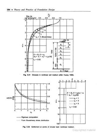
148. 128 • 17reory and Practice of Foundation
D~sign
(6. 19)
2.2
2.0
...
1.8
~
1.8
c
~
Smooth, Fs
1.2
1.0
0
•
8
12
16
20
0.05
0.03
!,.h'8
0.01 0
Fig. 8.10 Bearing capaelly of non-hOmogeneous toll {aflor Oavls and Brcol<or 1973).
where A is a parameter which depends on the roughness of the footing and ~ is the rate of
increase of c., with depth.
Davis and Christian (1971) analyzed the case of cross-anisocropic soil and found that
the value of c. may be talcen with sufficient accuracy. as
c, = o.{··; c,.)
(6.20)
where ''"' and c..,. are the undrained strength of the soil in the vertical and horizontal
direction respectively. Good prediction of bearing capacity of model footings in Boston blue
clay was obtained by using Eq. (6.20).
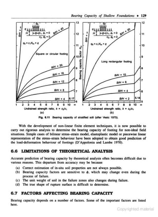
Vesic (197S) made detailed theoretical analysis of two-layer soil system, shown
in Fig. 6.11. with the bearing stratum either softer or stiffer than the underlying stratum.
In the first case. failure is partly by lateral plasLic now whereas in the second situation.
failure is caused by punching shear. The net ultimate bearing capacity of the footing is given
by.
(6.21)
where Nm is a modified bearing capacity factor which depends on the ratio of shear strength
of the two strata and the thlckness of the bearing stratum and is given as
Nm = {k(k + l)N; + k + {J - l][(N; + {J)N; + {J - I] - (kN; + {J - I)(N; +I)
(6.22)
Copyrighted material

149. B<aring Capacity of Simi/ow Foundations + 129
q
I
II
12
10
9
long rectangular footing
I
2
3 •
5 8 1 8 9 10
lJnctrWntd lll'ength l'lllo, k • cic,
G
(a)
Fig. 8.11 Beoring capacfty of sntlfled sdll (oftet 1/eslc 1975).
With the development of non-linear finite element techniques. it is now possible to
carry out rigorous analysis to detennine the beMing capacity of footing for non-ideal field
situations. Simple cases of bilinear stress.-sttain model. elastoplastic model or piecewise linear
representation of the stress.-strain behaviour have been adopted to obtain good prediction of
the load-<leformation behaviour of footings (D'Appolonia and Lambe 1970).
6 .6
LIMITATIONS OF THEORETICAL ANALYSIS
Acx:urate prediction of bearing capacity by theoretical analysis often becomes difficult due to
various reasons. This depanure from accuracy may be bec.au.sc
(a) Correct estimation of in-situ soil properties are not always possible.
(b) Bearing capacity factors are sensitive to ;. which may change even during the
process of failure.
(c) The unit weight of soil in the failure zones also changes during failure.
(d) The true shape of rupture surface is difficult to detennine.
6 .7
FACTORS AFFECTING BEARING CAPACITY
Bearing capacity depends on a number of factors. Some of the important factors are listed
here.
Copyrighted material

150. 130 • Theory and
Practic~
of Fouttdalion Design
(a) Subsoil stratific~tion and properties.
(b) Type of foundation and geometric details s uch as size, shape, depth below ground
surface, eccentricity of loading and rigidity of the stnlcture.
(c) Pennissible settlement.
(d) Location of ground water table.
6.7.1 Effect of Ground Water Table on Bearing Capacity
The position of ground water table has a very important effect on bearing capacity. For
clayey soil if the water table is near the ground surface and the soiJ is saturated, ; = 0 under
undrained condition. If the water table is at depth equal to or greater than the width, B
below the level of footing, then the soil is partially saturated and total stress analysis,
considering both c and ;, may be urried out. For conservative estimate, ; = 0 analysis is
carried out assuming water table at ground surface to take account of seasonal variation in
water table. The ultimate ~g capacity is taken as, Skem)l(on (1951),
qd = eN, + yDI
(6.23)
where y is equal to the ~turated unit weight, y,...
But, for granular soil effective stress analysis is appropriate. The bearing capacity
equation for strip footing on sand is,
(6.24)
where y' is the effective unit weight and N, and N1 depend on ;•. Here, y ' depends on the
position of water table, as depicted in Fig. 6.1 2.
FJg. 1.12 Effect of groood walef table.
For the strip footing shown in Fig. 6.12, the depth of failure surface does not extend
beyond a depth equal to the width of the footing 8 below the footing base. If the water table
is at or beyond this depth, it will have no effect on bemng capacity. If the water table is at
the base of the footing or above, then in the second tenn of Eq. (6.24) r ' =
which is
about half the value of y,... The second term of Eq. (6.24) can now be written as
(I/2)RwyBN7 where Rw is a water table correction which may vary from 0.5 to I and c.an be
expressed as
r:.•.
Copyrighted material

151. B~aring
R. =
Capacity of Shallow Foundalion.s
t
o.s(
~)
(6.25)
I +
131
where D. is the depth of water table below the base of footing.
Likewise, first tenn of Eq. (6.24) can be written as (R'wrD1N~ where R~ is a water
table correction factor, which may lie in the range (0.5- 1) and may be expn:ssed as
R',. =
o.s(1 + ~;)
(6.26)
where fY. is the depth of water table below ground surface.
Thus. to take effect of water table. the bearing capacity equation for a strip footing on
gmnular soil may be expressed as:
q,
= R'.rv1N, + o.sR.rBN,
(6.27)
where y is the bulk unit weight, and R..,. and R:. are the water table correction factors which
may vary from O.S-1.
A pmc.tical method of considering the effect of ground water table is given in Chapter 8
(Section 8.2.3)
6 .8
GROSS AND NET SOD.. PRESSURE: SAP'E BEARING
CAPACITY
The tool pressure transmitted to the subsoil by a foundation is the gross soil pressure. and
the maximum gross pressure at which the soil fails is known as the ult;IIIQte gron bearing
capacity. At the level of foundation, which is at a depth D1 below the ground surface, the
overburden pressure is yD1 The soil at this level was under this pressure prior to the
application of footing load. The pressure transmitted by the foundation in excess of the
overburden pressure is the net bearing pressure. The maximum net pressure at which the
foundation faiJs is known as ultimate nd ~Haring caf)Qdty. Safe bearing capacily is the
maximum intensity of pressure which the soil can support without the risk of shear failure.
This is obtained by dividing the ultimate bearing capacity by a factor of safety. Since the soil
is originally subjected to the overburden pn:ssure yD1, then: is no need to apply a factor of
safety to the component of gross bearing capacity which is due to yD1
Therefore.
q (all) = q,h(•l + yD
'
Fs
7
It may be noted that there is a difference between safe bearing capacity and allowable
bearing pressure. The allowable bearing pressure is the maximum net pressure that can be
applied on the soil without the risk of shear failure or settlement beyond permissible limits.
6 .9
BEARING CAPACITY FROM FIELD TESTS
Fo< granular soils. estimation of field value of ; from laboratory test is extremely difficult
It is more convenient to estimate ; from results of penetration tests, for example. N value
Copyrighted material

152. 132
+ 17"ory and Practice of Foundation Design
from SPT. N, value from dynamic cone penetration test, or q, from static cone penetration
test. Methods ase also available to compute bearing capacity direc~y from penetration test
results. Some of these methods ase as follows:
I. Using chans given by Peck, Hansen, and Thombum (1976}:
Figure 6.13 is a plot of bearing capacity factors, N, and N1 against ' as well as N
value (corrected). Considerations of both general and local shear failures are
incorporated in the clwt. This chart can be used direcdy for N, and N 1 (according to
Terzaghi's method) for use in bearing capacity equation, Eq. (6.8).
,.
0
'
......
120
.. . ....
-IO<Y
rLoooe
II
0
N
I
20
!
').,
I"'
i
!
I
!
''
l' .
! '
N,,
: I
I /.'
: .''
''
N,
'
Jfl
,,
20
~7,·
32
36
40
44 46
Anglo of inlomal friction. • degrees
Fig. 8.13 Bearing capedty of looCings based on 'N' valUe.
2. Teng 's Formula.:
Using the concept of Peck, Hansen, and Thombum , Teng (1962) developed the
following expression for calculating net ultimate bearing capacity on granular soil.
For strip footing,
q,. =
~ [3N1 sw; + 5(100 + N 1 )D1 w;J
(6.28)
For square or circular footings.
(6.29)
Copyrighted material

153. Btaring Capaciry of Shallow Fou11dations + 133
where
q,.d = net ultimate bearing capacity in t/m2 or kN/m2 .
N
average N value com:cted for overburden pressure.
D1 = depth of footing in metres; If D1 > B. take D1 = B.
W~ and
= correction factors for water table.
=
wy
3. Static
con~ t~st:
IS:6403-1981 gives a method of determining net ultimate bearing capacity of strip
footings on cohesionless soil using static cone resistance. q". The chart is presented
in fig. 6. 14. q~ values at different depth are obtained for selecred locations at the
site. The fie ld values are com:cted for the dead weight of the sounding rod. Then
the average q, value is obtained for each of the locations by averaging the values
between the base of the footing and depth below the base 1..5-2 limt$ the width of
the footing. The smallest of the average values is used in Fig. 6. I I to find bearing
cal"'city factors N, and N,. which may be used for computing the bearing cai"'City.
0~--~~--~~--~--~
0
100
200
300
B
(em)
Fig. 6.14 Bearing copacfty 11om static cone Int.
Example 6.1
A square footing of width 2 m re.~ts at a depth of 1 m at a site where the subsoil consists of
soft to medium clay down a depth of 8 m below ground level, which is underlain by a dense
coarse sand deposit. The water table is at l.S m below G.L. The clay has c. = 30 kNim1.
9 = 0 and = 19 kN/rn 3.
Determine the net load the footing can safely carry with a factor of safety of 3 against
shear failure. Vhat will be the safe load if the wotcr table rises to the ground surface?
r
Solulion
Since the thickness of clay layer beneath the level of footing base is more than the width of
the footing. the bearing capacity will be governed by upper layer of clay.
Copyrighted material

154. 134 + Theory and Practice of Foundation Design
According co Skempton's fonnula
(q,.),.. = c.N,
N, = 6( 1 + 0.2D 1B)
1
Here,
= 30 x 6.6 kN/m2
= 6.6
(q .,,,),..
=
30 X 6.6
2.5
= 2.5)
(Fs
= 80kN/m2
Net safe canying copocity of the footing = 80 x 2 x 2
= 320 kN
Since this is a total stress analysis, there will be no change in the safe load if the water table
rises to the ground surfoce, unless there is a change in strength of the clay.
Example 6.2
The subsoil at a building site consists of medium sand with y = 18 kN/ml. c' = 0, ~· = 32°
and water wble at the ground surface. A 2.5 m square footi ng is to be placed at 1.5 m below
ground surface. Compute the safe bearing capacity of the footing. What wouJd be safe
bearing pressure if the water wble goes down to 3 m below G.L?
Solunon
Since ,. lies between 28° and
35~
the bearing capacity factors are obtained by interpolation
between local and general shear failure conditions.
Refening to Fig. 6.7, for 9' = 32°, Nq = 28. N', = 10, N1 = 30. Ni= 6
= 10 + [
18
;~ 2-- 2 ; 8)] = 20.3
we get.
N,
and
Nr = 6 + [24i;2
-2~8)) = 19.7
Cas. I (water lJible at G.L.)
Using Eq. (6.27) modified for square footing, ultimote gross bearing capac ity
(q,,.)1..,, = y'D1N, + 0.4y'BN1
: 8.0 X 1.5 X 20.3 + 0 .4
X
8.0
X
2,5
X
19.7
= 243.6 + 157.6 =401.2 kN/m2•
and ultimate net bearing capaciry.
(q,"),,.. = (q,,.>...,.
-
= 40 1.2 - 18
rDt
X
1.5 = 384.2 kN/m2
Copyrighted material

155. B•aring Capacity of Shallow Foundations • 135
Safe net bearing capacity.
(q.,1,).., = 384.212.5 = 152 kN/m2
(Fs = 2.5)
and gross bearing capacity,
(q..rJ.,...
= 152 +
18 x 1.5
= 179 kN/m2
Case II (Water table at 3m below G.L., that is, at a depth greater lhan width footing)
(q.,J.,....: 18
X
1.5
X
20.3 + 0.4{14
X
2.5)19.7
= 548.1 + 275.8 = 823.9 kN/m2
(q.1
,),.. = 823.9 - 18 x 1.5 = 796.9 kN/m2
safe net bearing capacity.
(q..rJ... = 796.912.5 = 319 "320 kN/m2
and safe gross bearing capacity,
(q..rJ..- = 320 + 18 x 1.5 = 347 =350 kN/m2
(This problem may also be solved using water table correction factors W~ and W' with
1
marginal change in the result Also Fig. 6.10 may be used for obtaining relevant N 9 and N 1
values.)
Example 6.3
A rectangular footing, with a plan area of 1.4 m x 2 m is to be placed at a depth of 2m
below the ground surface. The footing would be subjected to a load inclined at 10" to the
venical. The subsoil is clayey, sandy silt with saturated unit weight of 18 kN/m3, and
c' = 10 kN/m2 and ~ = 30°. Assuming the rate of loading i.s such that drained condition
prevails, compute the magnitude of load the footing can carry if the water table is at the base
of the footing. Use IS: 640>-1981 recommendations and take Fs = 3.
Equation (6.13) gives,
q_, = cN.s, d, i, + q(Nq - l)s•d•i• + O.Sy8N1 s 1 d1 i 1 W'
Here c = c' = 10 kNim'. ; = ;• = 30°
N• = (e",.. 0 )tan 2(45° + ;12)
N, = (N. - l)cot;
= 18.38
= 17.38cot30°=
30.10
N1 = 2(Nq + I) tan;= 22.37
s, = I + 0.28/L = 1.14
sq
= I + 0.28/L = 1.14
s1 = I - 0.48/L = 0 .72
If. =
1 + 0 .2Dtf8tan (45° +
;n> = 1 + 0.2 x 2/1.4 x 1.732 = 1.5
Copyrighted material

156. 136
t
11reory a11d Practice of Fomulntio, Dtm'g11
d, = d 1 = 1 + 0.1D1 tan (45° + frl) = 1 + 0.35/1.4 = 1.25
i,
= ;, = (1
- a/90)1 = 0.79
iy = 0.44
W' = 0.5
Hem:e.
q..,: ( 10
30.J X J.l4
0.79) + (0.5 X 18
X
X
X
J.5
1.4
0.79) + (18 X 2 X (18.38 - 1) X J.l4
22.37 X 0.72 X 1.25 X 0A4 X 0.5)
X
X
X
J.25
X
= 406.6 + 704.4 + 55.8 =1166.8 kN.
(q..J..t. = 1166.813 = 388.9
2!
380 kN/ml
Hence, safe load = 380 x 1.4 x 2 = 1064
2!
1060 kN
Esample 6.4
Wbat will be lbe safe load in Example 6.3 if undrained condition prevails? Take c. = 30 kN/m2,
0, N, 5.14, N, =I, and N1 : 0.
;,. =
=
St>iuJU>II
: 30
X
5.14
X
1.14
X
1.5
X
0.79
= 208.3 kN/m2
kN!m 2
(q ..J..r, = 208.313 = 69.4
2! 70
Safe load : 70
= 196 kN
X
1.4
X
2
2! 200 kN
Brinch Hansen. 1. (1961). A General FomJUla For Bearing Capacity, Danish Geotechnical
Institute, Bulle.tin No. 11 . Copenhage.n.
Brinch Hansen. 1. (1970). A Revised and Extended Fomru/a for Bearing Copaciry. Danish
Geotechnical Institute, Bulletin No. 28, Copenhagen.
Davis and Brooker (1973), The Effect of Increasing Strength with Depth on the Bearing
Capacity of Clays, Geottchnique, Vol. 23. pp. 551-.563.
D'Appolonia. D.J. and T.W. Lambe (1970). Method of Predicting Initial Settlement, Journal
Soil Mechanics and Foundarwn Division. ASCE. Vol. 96. pp. 523-544.
IS 6403 ( 1981). Codt of Practice for Dettnninarion of Bearing Capaciry of Shallow
Foundations. Bureau of Indian Standards, New Delhi.
Meyerhof. G.G. ( 1951), The Ultimate Bearing Capacity of Foundations. Geottchnique,
Vol. 2. pp. 301- 332.
Copyrighted material

157. Btaring Capacity of Shallow Foundations • 137
Peck, R.B., W.E. Hansen, and W.H. Thombum (1962). Foundation Engineering, 2nd
Edition. John Wiley & Sons. New York.
Prandtl, L (1921). Uber die Endvingungs Festingkite von Schneiden, 'kirsclrrift fur
Angebandrt Mathtmatik and Mechanik, Vol. I, No. I , pp. 15-22.
Reissner (1924). Zuns Erdd,.,ck-problem. Proc. Fint Int. Congress on Applied Mechanics.
Dept. pp. 295-311.
Skempton. A.W. (1951), The Btaring Capacity of Clays. Building Research Congress,
England.
Terzaghi. K. (1951),
7l~eoretical
Soil Mtchanics. John Wiley, New York.
Vesic, A.S. (1973). Analysis of Ultimate Loads of Shallow Foundations, Journal of Soil
Mtchanics and Foundation Division ASCE, Vol. 99, No. S M I, pp. 45-73.
Vesic, A.S. (1975), Bearing Capacity of Shallow Foundations. · Chapter 3 of Foundation
Englnetrlng Handbook. Van Nootrand Reinhold Co., New York.
Copyrighted material

158. Settlement Analysis
7.1
INTRODUCTION
Foundacions on soft clay are liable to undergo excessive settlement and prediction of this
settlement is an imponant aspect of found<ltion design. A part of this settlemen~ known as
the immediate settlement,, is a result of undrained shear deformation of the soil and takes
place during loading. A major part of the settlement. however, occurs due to volume change
of the clay Cllused by the dissipation of excess pore pressure developed from imposed loads.
This is a gradual process and is known as primary cotuolidaticn. ln addition, there may be
settlement due to secondary consolidation caused by volume change of the clay apparently
under constant efFective stress. Except in clays which exhibit high secondary effec~
settlement analysis usually involves an evaluation of the immediate and primary consoHdation
settlement only.
Soft clays, in general, are normally consolidated and their behaviour differs somewhat
f<om overconsolidated clays and clay shales. A survey of case records of seulement of
shallow found<ltions on clay (Simons and Som 1970) reveals that structures founded on N.C.
clays, in geneJal. experienc~ more senlement than those founded on overconsolidated clay.
This· is only to be expected because the main effect of overconsolidation is to reduce the
compres.sibilicy of the clay. However, it is more imporcant. that for normally consolidated
clay. only 15-20% of the total settlement occurs during construction. whereas for
overconsolidated clays. as much as 50-60% of the wr.al settlement may occur during
construction. This shows the imponance of consolidation on the settlement of foundations on
clay and evaJuation of this settlement becomes a major part of the settJement analysis.
7 . 1.1 Defl.nitions
Figure 7 . I shows the development of net pressure and the associated settlement of o
found<ltion on clay during different stages of construction. Before application of the building
load. there is usually an excavation down to the foundation level during which lhere is a
heave of 1he subsoil. The ml_gnitude of this heave is generally small. unless the excavation is
deep and is kepi ope- fot a long time. After excavalion. lhe foundation load is gradually
n
applied and there comes a time when the applied pressure on the soil equals the pressure
1 58
Copyrighted material

159. S~ul~m~Jll
Analysis + 139
re l ea~d by excavation and the net foundation pressure becomes zero. The corresponding
settlement due to !he restoration of !he excavation load may be assumed to be equal to !he
prior heave. Any further increase of load is a net increase in foundation pressure and the
associated settlement is the net settlement of the foundation.
..
•
li
..
~
i
;;
z
c
'
p,
!Wve
p,
lmmedia1e setlement
1
s
<!:
Consolklation
&elllement
~
+
<t
p,
"
.s:
Fig. 7.1 Tmo-oei1Jement relationship ol toundatJons on clay.
When the construction is complete and the total building load has been applied. the
immediate settlement. p, has already occurred. If the construction is rapid this settlement is a
result of shear defonnation of the clay. For a saturated c lay. this occurs essentially under the
condition of zero volume strain. Any consolidation seuJement at thi$ stage is small.
After the construction is over. the clay undergoes consolidation and the settlement
graduaHy increases with time unlil, lheorelica11y. a frer infinite time. rhe consolidation is
complete. The total consolidation settlement. p, is then added to the immediate settlement,
f>i, to give the final senlemenr. p1 of the foundation. Therefore.
Pt=P; + p,
(7.1)
7 . 1.2 Me thods of Settlement Analysis
The principle of effective stress :md Tenaghi's theory of one<-d1mensional consolidation have.
been the essential basis for settlement analysis of foundations rounded on clay. The earlies1
method of settlement analysis for a foundation placed on a layer of clay is shown in Fig. 7.2.
The sett1ement is given by the equation,
.
Pr- =
Jm.., dat dr.
(7.2)
0
Copyrighted material

160. 140 • Theory and Practice of Fou11darion Desigu
Net foundation
pressure q.
I
z
~$
I
I
Deplh
I
where.
m.., is the compressibility of the clay as determined from one-dimensional
consolidation test.
C.a: is the increase of vertical stress at the centre of the layer, and
dt is the thickness or the clay layer.
The method was proposed by Terzaghi (1929) for obtaining the consolidation settlement
of clayey strata subjected to lateral confinement. that is. where all settlement is due to one-.
dimensional compression of the clay. Although this method. is valid only in cases where the
condition of no lateral strain is at least approximately valid il has been extended to cases in
the field where the roondation rests on a deep bed or clay (Taylor 1948). In such cases. there
is lateral defonnation during load application which gives rise to 'immediate' settlement.
Therefore. the conventional method seems physically inadequate to describe completely the
behaviour of a clay that undergoes important lateral deformations.
Immediate oettlement
lc is now the common practice to obtain the 'immediate settlement'. that is, the settlement
that takes place under undrained condition due to the shear deformation or rhe clay, from the
equations or elasticity. This has the general expression (given by Terzaghi ( 1943)).
_ ( q.B(1 £
P;-
v') )
1p
(7.3)
Copyrighted material

161. Settlemenl A.twlysis • 141
where.
q, is the net (oundation pressure.
8 is a width of the foundation,
£ is the Young' s modulus of the clay.
v is the Poisson·s ratio. and
lp is the influence coefficient whose magnitude depends on the geometry of the
foundation.
The values of fp for different values of UB for rectangular foundations are given in
Table 7.1. For rigjd foundacjons, lhe influence coefficient may be taken as:
(7.4)
(/p)RJOID; 0.8(/p)CEI<TRE
Tablt 7.1 Values
111 •
or influence: coerf.eicnt lp for rectangle foundation. L x B
Valt~~u
UB
Ctnlrr
t.O
t.S
I.S2
1.78
4.0
s.o
t.96
2.to
6.0
7.0
2.24
2.32
8.0
2.42
9.0
2.SO
tO.O
Circl~ Oia. B
Comu
l. t2
t.36
2.0
3.0
ofJ
2.53
1.00
0.64
Because of sample disturbance. values of E ob~ned from laboratory triaxial compression
tests are often unreliable. h is preferable to obtain E values from plate load tests made in the
field or from established empirical relations of E and the undrained shear strength, c,, of the
clay. Butler (1974) gives Elc. ratio of 400 for ovcrconsolidatcd LDndon clay while Bjerrum
(1973) gives the c,/p ratios in the range of SOO to 1SOO for nonnally consolidated clays, based
on measurement of undrained shear strength of the clay by the vane shear test.
For foundations placed at some depth beneath tbe ground surface. a 'depth correction'
may be applied to the settlement calculated by Eq. (7.3) (Fox 1948). The depth correction
depends on the depth to width ratio and length to width ratio of the foundation. Values of
the depth correction. given in Fig. 7.3. are de,fined as
settlement of foundation at depth D
Depth correction factor = ---:-..:..:.=c=c=..:..:.c..:.===..:;;,..:..:.";;'-'-"-.,-,...selllement of corresp<>nding surface foundation
Copyrighted material

162. 142 + Tireory and Practiu of Foundatio" Design
Oepl.h fJeror "'
850
060
0 70
0.80
0.1
090
00
2
10
~
o. t=:"[~=rr::!:::::!:~~~~~4~
0
25
9
0.3 -
O.•~w~~~:~.~·trt 2jf,'-~tj
· ~ ~5~,~ " tl
f
r.; 0.5~
r;;
0.6f--t-++-+--t-lll'f-l--t-+--l
D
+ifr
0.7
O
.BI-f--+-t-t- -t---1-t--H
-Jfi
o
.9f--+-+-+--l---,f--+-+-+--lH
1
.0f--t-++-+- - t---+-+-+-l
r71r
Y/11
fjft 1--1--1--1--1--l
-
0.9
0.8
I
0.7
Jib
{)
IN
o.6f--+-+ -tffl'--f--+-+-+--lH
I II~
IJ'I --l---1-- 1 --l---f---1
0.4 f--+--f'-,1/
,Ht,f-l
o.5f--+--+~fH+-+-+--lf--+--+--l
1-., 1
1 . Numbers denote rotio olb
o.a~::;t;tY.tl:~lllltl
I 9 I/ .
25
1
Fig. 7.3 Depth oorreetlon faetor.
ConsoUdatlon aettlement
While Eq. (7.3) still remains the most widely used expression for calculating the immediate
senlemen~ the method of obloining the consolidation senlement has undergone some changes.
Skempton and Bjerrum (1957) recognized that there was lateral deformation in the c lay
during load application and that the consolidation settlement should be a func tion of the
excess pore pressure set up by the applied load. Therefore. taking accounc of the shear
s tresses. a modified expression for the total settlement was given as,
Pt = P; + JJP.,o
(7.5)
Copyrighted material

163. Stlllement Analysis • 143
where
11 is lhe pore pressure com:ction factor which depends on lhe pore pressure parameter
A and the gcometty of lhe foundation and
p..., is lhe consolidation settlement obtained by the direct application of the nedometer
test results (Eq. (7 .2)).
The values of pore pressure correction factor as given by Skempton and Bjenum (19S7) are
given in Fig. 7.4.
"tB • ..o.~
"~ -~ -
--
.....
...
0.21----11----+---+----'-------l
-
Circutar b.Jndation
·--·· Continuous foundation
O·L-----~----~~----~----~~--~
0.2
Fig. 7.4
0.4
0.6
0.8
1.0
Pen presswe cxwrection factor for rooodations on day (after Skemp4on and 8jerrum 1957).
For routine design. the following values of the pore pressure correction factor may be
used:
Normally consolidation c lay
Overconsolidated clay
Heavily overconsolidated clay
7 .2
1.0-{).7
0.7-0.5
0.5-0.3
STRESS-PATH
It is well-recognized that the deformation of an element of soil is a function not only of
magnitude of the applied stresses but also of the manner of their application. In other words,
a knowledge of the magnitude of stress in<:reasc is not. in itself. sufficient to indicate
precisely how a soil element is going to deform. To obtain a more complete picture. we have
also to know how the applied stresses change. at what rate and in what relation to one
another (Som 1968).
Copyrighted material

164. 144 • TMory and Practiu of Foundation Design
A stress-path is essent.ially a curve drawn through points on a plot of stress changes. It
shows the relationship between the components of stresses at various stages in moving from one
stress point to another. In the present study, however. consideration is given only to cases where
by virtue of symmeli)'. the intermediate and minor principal stresses are equal and where the
vertical and horizontaJ stresses are the principal stresses, for example~ in the laboratory triaxial
test or along the centre Hne beneath a loaded circular area. In its natural condition, before any
load is applied, an element of soil is in a K. state of stresses (K0 = coefficient of earth pressure
at rest). Depending on whether the soil is normally consolidated or overc,onsolid.ated the
horizonlal stress in-situ may be smaller or greater than the vertical stress.
Let us consider an element of clay beneath the centre of a uniformly loaded clrcle. as
shown in Fig. 7 ..S. The in-situ effeetive stresses (p and K,p) are represented by the point ' A'.
Due to the foundation pressure, q, the stresses on the element increase by flu, and flo-.,. If
the pressure is applied sufficiently fast so that no drainage occurs during the load application,
the element deforms without any volume change and any vertical compression is associated
with a lateral expansion.
•u
A B Cl_ Efleetlve
A8
Qf stress-9ath
4a;;
Fig. 7.5 Sbeu-path of an element of soli beneath founc:taliOn In the fiekS.
Now, the increase of stresses Aa. and Aa111 • which are the increase in principal stresses
in this instance, will set up an excess pore-water pressure in the element according to the
equation,
bu = B [flo-At + A (flo-.- flo-.,)
(7.6)
where A and B are S kempton's pore-pressure parameters (Skempton, 1954).
If the clay is saturated, as all clays below the water table are, B = L Then,
bu = flo-At + A (flo;, - flo-.,)
(7.7)
Therefore, immediately after the load application, the effee.tive streSSes become:
o-;o = p + flo-.- flu
o-;o
= K0 p + flo-At - flu
}
(7.8)
Copyrighted material

165. SettletMnt Anolysis • 145
Since for lllOfit clays, the value of A is positive in the range of 1tres.ses normally encountered
in practice, the excess pore-pressure t.u is greatct lhan t.o-., . So while the effective vertical
stress increases on load application, the effective horizonaal sll'US decreases and the slreSS
point moves from ' A' to ' 8 '. The venlcal sltlln during, loading. that is. the immediate
settlement. is, therefore, a function of the stre"'palh AB.
The element now begins 10 consolidate. At the early saages of consolidation. the
increase in effective horizontal StresS is only a recompressioo until the original value lc.P is
reston>d. Beyond this point, any funher increase of horizontal 5treu is a net increase while
there is a net increase in vertical StresS durin& the entire process of coosolklation.
Now during load a.pplicalion, in undrained eondltion. a utunued clay behnu as an
incoiDJI"'SSlble medium wilh Poisson's mio, v • 0.5. As the excus pod-pressures dissipate.
Poisson's ratio decreases and finally atUlns iu fully drained value at the end of OCli1SOIKialioo.
This ebange in Poisson's ,.tio does 1101 have much effect on the vertieal stress but the
horizontal StresS decreases by an amount 6 to ha new value K,p + bc>u. i..,.,
6 • t.o-,. 1
-
t.u.,
(7.9)
So during consolidation. the element follows the effective wess palh BD while it would
have moved from 8 10 C had the total StresS remained unehansed. A&r full consotidation.
lherefon:. the stresSes are:
a;,. • t.o.
}
0"'¥ • K. p + (t.o-., - 6)
(7. 10)
• K. p+ 6o61
An ideal seulement analysis should take into account !he complete pauem of suesses an
element of soil will be subjected to in the field. In order to determine the relevant venical
sltlins, laboratory tests should be performed under Identical suess conditions and an
integration or all s-uch venica.l strains beneath a loaded area would give the settlement of the
foundation (Lambe 1964, Davis and Poulos 1967).
The methods most widely used in pracclcc. however. are the ones based on the
oedometer test. Figure 7.6 summarizes all these melhods indicating lhe effective stress-paths
associated with each of them. In plotting the stre..·palh AF in Fig. 7 .6, it has been assumed
that an undisturbed sample when subjected 10 the In-situ vcnical stress also restores the insitu horizontal stress so lhat subsequent stress-path for loading sUirts from lhe point A .
....
MlhJd
I
2
3
•
Fljj. 7.1 ..._
....-
....
~
Streu-o~~th
AF
AS, M'
AS. EF
AS, 80
...,
ln'c>llod ..............

166. 146 • Tlreory and Practice of Foundatiotl Design
Method I, described by Skempton and McDonald (1955) as the conventional method,
was first proposed by Tcrzaghi (1929) and later used by Taylor (1948). It a.,gumes that all
settlement occurs from one-dimensional compression and that the excess pore-pressure is
equal to lhe increase in verticaJ sttess. Therefore. the corresponding stress-path is ~Method 2 recognizes that the soil undergoes shear deformation during undrained loading
(path AB). and this causes the immediate seulement, but still assumes that the excess
pore-pressure, which should be a function of the induced shear stress~ is equal to the vertical
stress increment. Consolidation settlement. therefore. occurs along the stress- path AF. This
inconsistency in Method 2 has been overcome by Skempton and Bjerrum (1957) in Method 3.
Here. the immediare settlement is a function of the stress- path AB whiJe the consolidation
settlement occurs along the path EF. The latter. therefore. is only a part of the total strain
along the path AF depending on the magnitude of the excess pore-pressure set up during
loading.
While the method of $kempton and Bjerrum introduces for the first time, the concept
of strcss,.path in settJement analysis, the as."umption ls still implicit that during consolidation
all strain is one-dimensional ·which requires the horizontal stresses to adjust accordingly.
Therefore, there is a discrepancy between the field stress-path 80 and the path EF used in
the analysis. The condition of no lateral strain may be approximately true in cases like that
of a loaded area which is very large compared to the thickness of the clay layer. But in the
majority of field problems. this condition may be far from ltue. Moreover. while computing
the immediate settlement. Method 3 obviously accepts that the clay undergoes lateral
dcfonnation during loading (with constant volume, there would he no set~ement otherwise)
but th.is is neglected in estimating the consolidation seulement. Consequently, of course. the
effect of the horizontal stress is completely ignored except in determining the e xcess
pore-water pressure.
7 .2.1 Stresses During Loading and Consolidation in the Field
It is evident that during load application in the field. most of the defonnation takes place
under condition of no volume change, implying a value of Poisson's ratio of the soil equal to
0.5. As the excess pore-pressures dissipate. Poisson' s ratio also decreases and finally drops to
its fully drained value. It is known that for an isotropic homogeneous e lastic medium. the
venicaJ stresses are independent of the elastic parameters and are. therefore. unlikely to be
significantly affected by this decrease in Poisson's ratio. On che other hand. Poisson's ratio
has a cons-iderable influence on the horizontal stresses even for the Boussinesq case beneath
the centte of a uniform circular load. Therefore, it is clear that the problem of consolidation
in the field is very much interlinked with the problem of stress distribution, whose rigorous
analytical treatment is extremely complex. An approximate analysis may he made on the
assumption that the horiwntal stress at the e nd of consolidation will be the same as the
Boussinesq stresses for the appropriate value of Poisson's ratio.
If we consider an element of clay at a certain depth where. during load appliealion, 60'.,
and 60'111 are rhe increase in vertical and horizontal stre.'.Ses respectively lhen, at the end Or
consolidation. the venica1 stress will still remain unchanged but lhe horizontal stres.~ will
have decreased to the new vaJue 6a111 due to the reduction of Poisson's ratio.
Copyrighted material

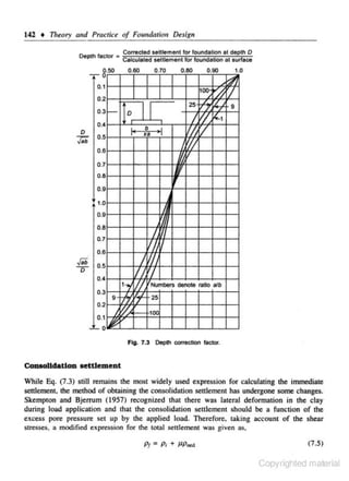
167. S~ttl~m~nl
Analysis • 147
So. the changes in effective stress during consolidation an: given as
[6u,l, =
Horizontal:
11.u-
6
(7 .11 )
Vertkal:
where
6 = 6u, 1 - 6a.,.
The ratiO of the effective stress changes during consolidation, K' is then given by
K'
=
[Au,J.: • I - .!.._
[Aa,l,
(7.12)
6u
Now. for the Boussinesq problem, the general expressions for stresses beneath the centre of a
uniform circular load (dlameter 2b and load intensity. q) are (Wu 1966),
u _
' - q
[I _
(tlb)
3
]
(I + t 2/b2 ) 311
(7.13)
3
a = !l.[(l + 2v) _ 2(1 + v)(tlb) +
(t/1>)
]
'
2
(I+ z2 /l?)
(I + z3/b3 ) 311
which can be more conveniently written as,
u, = q(l - '1')
u, = ~((I + 2v)- 2(1 +
V)'l
+ '1'1
(7. 14)
where.
(7.15)
Using these expressions,
Aa, = (u, ),. 111 = q(l - 11'>
6a,, = (u,),. 112 = ~ [2- 3'1 + 11'1
(7.16)
6u., = (u,), . .. = ~[(I+ 2v') ~ 2(1 + v') '1 + 11'1
Combining Eqs. (7.13) to (7. 16). we have
K' _ I _ [
I - 2v
]
I + IJ{l + 1J)(3A - I)
(7 .17)
Eq. (7 .17) can then be used co determine the mt.io of the s
tress increase during consolidation
at any depth beneath the centre or a uniform circular load.
Copyrighted material

168. 148 • Theory and Practice of Foundat;o,
7.2.2
Desig~t
In1luence of Stress-path on the Drained Deformation
of Clay
It has been shown in the foregoing that the stress changes thai occur in the field during
consolidation are primarily dependent on the drained Poisson's ratio and the pore pressure
parameter A of the soil. Therefore. it is of considerable practical significance to study the
influence of scress-path, such as BD (sec Fig. 7.5) on che axial and volumetric strain ·during
consolidation. Expcriment· J investigation with undisturbed London clay (Som. 1968).
a
normally consolidaced KaoliniiC (Das and Som e1 al., 1975) and undisturbed Calcuna clay
(Guha, 1979) show lhol lhe stress incrcmcnc mtio during consolidation has importanl effccc
on the deformation characteristks of the soil. Two things need to be considered here:
(a) the influence of stress incremenl mtio on lhe volumetric strain of the soil and
(b) the influence of stress increment ratio on the strain ratio (that is, axial strain/
volumetric Slnlin) of the soil.
There is conflicting evidence on the effect of s tress ratio on the volumetric
compressibility of clay. Some investigators have found that the volumetric compressibility is
independent of the stress increment ratio and can be expressed as function of vertical
effective stress only (Som. 1968). This means !hat !he results of one-dimensional
consolidation ccsts would be applicable irrespective of the changes in lateral pressure during
consolidation. Others hove found that the volumetric compressibility is not independent of the
lateral pressure and can be$1 be expressed as functions of mean effective stress during
consolidation (Dos, 1975). It seems chat the appropriate relationship has to be determined for
the particular soil under investigation.
The major effect of lateral stresses during consolidation is, however. manifested in the
axial strain associated with volumetric defonnation. Figure 7.7 shows some typical results of
stress-path controlled triaxial tests on different clays. The results are plotted as relationships
between the stress increment ratio. K' and the strain ratio, A during consolidation or drained
deformation. It is to be noted that one~dimensional consolidation implies a strain ratio,
A= L.O nnd that occurs at a pank,ular stress increment ratio only. For any other. stress ratio.
the strain ratio would also the difference and assumption of one...cJimensional strain
(i.e. £ 11£., :: 1.0) would lead to significant error in settlement analysis.
4.0
3.2
2.4
1.6
1 Undistu'bed Calcufta day
2 Sedimented bolinite
3 UndisiUrbed London clay
Observed
- - - - · Theoretical (""Isotropic
elastcity}
"z
~
0.8
"~
~
-
-.
0.0
0.4
0.8
0.8
1.0
K' = Aa'.,IIJ.a ' 1
Fig. 7.7 Strain ratio, .t versus stress increment ratio. K· for draln~~~~!iq'£Xf
0.0
0.2
material

169. Seulemem Analysis • 149
The relationships shown in Fig. 7.7 can best be determined from stress controlled triaxiaJ
tests. However, Som (1968), Simons and Som (1969) have demonstrated that this relat.ions hip
can also be established cheoreHcally from considerarion of aniso1ropic elas1icicy as:
e,
I - 2~/,K'
£, = (I - 2v)) + 21)(1 - vj - Vz)K'
(7.18)
where.
v '1 = effect of one horizontal strain in the othe- horizontal scrain;
r
v'2 = effect of horizontal strain on vertic.al strain;
v'1 = effect of vertical strain on horizontal strain;
Jf = ratio of venical drained dcformatjon modulus to the horizontal drained
defoTITUition modulus.
Equation (7.18) can also be expressed as
I - 2~V,K'
£, = (I - 2v))[K'/K0 - 1)- 2~V,K'
£1
(7.19)
The parameters v'3 and rJVi can be detennined from two tests with different values of K' and
measuring £ 1/e., in each case. The most convenient values of·K' to choose are u and 1.0. that
is, !hose from lhe standard drained compression test and lhe isotropic consolidation test.
7 .2 .3
Settlement Analyala by Stre..-path Method
The methods of settlement analysis in current use have been described earlier. These methods
have given satisfactory results in many field problems, particularly where lhe condition of
zero lateral strain is satisfied. However, more often !han not appreciable lateral deformation
occurs in lhe field and lhe currently used methods of settlement analysis become inadequate
to predict lhe seulemenL A method of settlement prediction by the stress-path method has,
therefore. been introduced for lhe case of axi-symmetric loading (Simons and Som, 1969.
Som et al., 1975).
Immediate oettlemeat
The common practice in estimating lhe immediate (elastic) settlement of foundat ion on clay
is to assume the soil to be a homogeneous, isotropic. clastic medium. thus, permitting the
application of Boussincsq analysis. However, in practice, the elastic modulus~ E of tt:e soil
varies with depth as a consequence not only of the inherent non·homogeneity of the soil but
also of varying applied stress levels at different depths. Stress- strain relationship of soft clay
is essentially non-linear and the deformation modulus varies considerably with the stress
level. While it is possible to make theoretical analysis of undrained deformation using the
finite clement technique and taking the non-linear stress versus strain behaviour of the soil
into consideration, they are nor yet available in readily usable form. A ~il"ple expression for
immediate settlement following the stress-path method may be given as,
Copyrighted material

170. 150 • Theory and Pmctice of Foundation Design
_ 'JAa, - aa.
p, -
(1.20)
e(z)
0
where C.a. and La11 are the increase in toral vertical and horizontal stresses at any depth
re.•pectively and E{z) is the corresponding deforrru~tion modulus, taking due account of the
vertical and horizontal effective stresses prior to and at the end of loading.
It has been shown by many investigators that the stresses in the subsoil due to a
foundation loadjng are not significantly dependent upon the variation of E (Huang 1968.
Som 1968). Therefore. in the absence of more rigorous analysis. the Boussinesq stresses may
be used in evaluating the settlement by Eq. (7.21), the integration being done numerically by
dividing the compressible stratum into a number of layers and taking the appropriate value of
E for the layer into account.
Conaolldatlon aetUement
In the conventional method. the consolidation settlement is given by,
p,
•
J
=
(m,), a a, dz
(7.21)
0
where (m,) 1 is the coefficient of volume compressibility determined from standard
consolidation test and C.a: is the increase of vertical pressure at the centre of layer.
Following the Skempton and Bjerrum (1957) method, the settlement is,
p, = J.1
'J ) !!.a, dz
(m,
1
(7.22)
0
where J.1, the pore-pressure corTOCtion factor, is a function of the soil type and tbe geometry
of the foundation, (refer Fig. 7.4).
For the stress-path method. the settlement is given by,
p; =
•
J
).(m,)3 l!.udz
(7.23)
0
= ).p,
where,
tJ.u
= increase of pore-water pressure under undrained loading which dissipates
during the consolidation.
(m,h = coefficient of volume compressibility for three-dimensional strain.
A = the ratio of venicaJ strain to volumetric strain which is a function of the stress
increment ratio during consolidation.
If Eq. (7.23) is to be applied in seulement analysis, K' during consolidation needs to be
known in order to determine the value of A. Ac-eurate determination of K' for actual
foundation may be difficult becau,s e it depends on many factors such as Poisson' s ratio,
Copyrighted material

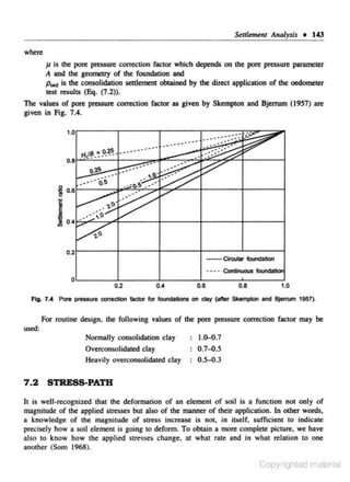
171. Seltlement Analysis + 151
pore pressure parameter A. stress-strain relationshjp of the soil. and so on. As an
approximation, however, its value can be determined from Eq. (7.17), for a footing of
diameter 2a. According to Eq. (7. 17),
K _ I _[
I - 2v
]
I + IJ(l + q)(JA - I)
where,
)-t/2
•'
1]= -< ( 1 + Q
a'
v = Poisson's ratio
A = Skempton's pore-pressure parameter
Knowing the value of K', A. can be obtained from experimental relationships as shown in
Fig. 7.7. The value of (m,):, should, of cour>e, be obtained from appropriate stress-path test,
bu~ for practieal purposes, can be determined from properly conducted oedometer test. Then,
(m.)) may be taken as approximately equal to (m,) 1, the oedometer compressibility in terms
of venical effective stress.
It may be noted here that evaluation of the K versus A relationship for any problem
requires determination of Poisson's ratio and pore-pressure parameter, A of the soil. But for
most soils, Poisson's ratio varies between 0.1 and 0.3 and pore-pressure parameter, A
between 0 and I. Accordingly, K varies within a narrow range of 0.6-0.9 and A in the range
0 ..5-0.8. It would, therefore, be convenient to select a value of l within this range for most
practical problems (Som, 1968).
7 .S
RATE OF SETTLEMENT
The rate of settlement of foundations on clay is generally determined from Tenaghi's theory
of one-dimensional consolidation although tield..:onsolidation is often three-dimensional (See
O!apter I. Section 1.9.5).
According to this, the excess pore-pressure at any point at depth t within a soil mass
after a time from load application, is governed by the equation
C lflu = 8u
'8:'
where~
8t
(7.24)
u is the excess pore·pressure and
C" coefficient of consolidation.
The degree of consolidation at any time, 1 (defined as the percentage dissipation of
pore-pressure) may be obraincd by solving Eq. (7.24) for appropriate boundary conditions.
Table 7.2 gives the relationship between time· factor, T, = C,JIH 2 and degree of
consoHdation, U for different boundary conditions.
Copyrighted material

172. 1S2 •
Tlr~ory
and Practice of Foundalion Design
Tablt' 7.2
U versus T~ relationship (T~ • C~t!H 1)
U%
(u,Ju,) • 0
o.s
1.0
s.o
T,
0
20
40
0
0.01
Cl.ll
o.os
0.049
0.64
0
0.014
0.081
0.19S
0.460
0
0.01
0.17
0.3 1
0.58
0
0.031
0.1 26
0.237
0.567
60
0.39
80
100
"'
"'
"'
"'
"'
0
O ISS
.
0.420
For double drainage (any distribution of pressure, that is, u 11u: :;:; any value). take
H = 112 times thickness of cJay and T,. values fo r (u 1/ui) = I.
7 .4
FOUNDATION ON SAND
Foundations on sand do not present the !>arne degree of problem with regard to settlement as
foundations on c;:lay. Firstly, except for loose sand. settleme- t is usually small and secondly.
n
because of high permcabilily the settlement is usually over during the period of construction.
In this case. there is no time dependent settlement similar to the consolidation settlement in
clayey soils. although large foundations may undergo minor settlement caused by fluctuations
of load due to wind, machinery vibrations. and storage loads.
a
Prediction of settlement of foundations on sand is, by and lange. empiric- l although
elastic theory has sometimes been used. The common methods used for this purpose are:
7 .4 . 1
Elastic Theory
The problem is similar to calculation of immediate settlement of foundations on clay as given
in Eq . (7.3). For a homogeneous. isotropic, e lastic medium
6 = q.B (I - v) 2 /
E
(7.25)
P
where the different terms have the same meaning as in Eq. (7 .3). However. it is to be
considered thac because of volume change during load application, Poisson's rutio. v can no
longer be taken as 0.5. The value of E and v should be determined from tbe laboratory triaxial
tests for the appropriate relative dens icy and confining pressure- The Poisson's ratio normally
.
varies between 0. 15 for coarse sand to 0.3 for fine to silty sand. The value of E can also be
determined from the standard penetration resistance or the soil (refer Otaptcr 2. Table 2.7).
Elastic theory. however, gives only a very approximate estimate of settlement, because
the assumption of homogeneity would be far from renlity.
7 .4 .2
Semi-empirical Method ()3ulsman, 1948)
Buisman (1 948) has given on empirical method or es timating the senlement of foundations
on sand by numerical integration of the strains occ urring in different strata. as s hown in
fig. 7.8. Accordingly.
Copyrighted material

173. Settlemtnt
log
10
Pu + l!.p dz
p.,
r
l l !
~)'Of
La)'llf
2
E,
z,
E,
z,
E,
z,
"'
Po • dl>
~
Layer 4
(7 .26)
l ! !
¢
¢
layer 3
• 153
Net foundation pressure, q,
~
1
llrr<~lysis
z.
Fig. 7.1 Settlement calc:aJiatlon for foundations on sand (after Bulsman. 1948).
where,
p. = initial effective overburden pressure befon: loading.
ap = increase of vertical stress at the centre of layer due to foundation loading,
E
= modulus of elasticity.
and
The sand layer is subdivided into a number of sublayers and the E values an: taken from
empirical relationship for the average N value for the layer, as described in Section 2,7.1
(Chapter 2).
7.4.3 Plate Load Teat
Tenaghi and Peek ( 1948) gave an empirical relationship between the settlement, S, of a
loaded plate of diameter. Dp for a given intensity of pressure and the settlement, s of a
1
fouodation of diameter, 0 1 at the same pressure. Bjerrum and Eggestad (1963) modified this
relationship as follows:
s,
S, = (I
4
+ D,ID ) 2
1
(7 .27)
The use or this equa!ion is based on the assumption that the density of the soil within the
zone affected by the foundation loading is similar to that beneath the test plate. This may be
approximately true if the plate diameter is of the same size as the foundation. but for large
foundations, there is likely to be considemble difference in density.
7 .4.4 Static Cone Test
If C~u~ is the point resistance measured by the static cone test, the settlement of the foundation
is given by the empirical relationship (Beer and Martens 1957).
Copyrighted material

174. 154 •
nr~ory
and Pract,.ce of Foundation Desig11
,.·
•
2.3H " '
o= --£.... I og Po + t.p
C
. (7.28)
Po
=
where, coefficient of compressibility, C
where,
= scatic cone resisc
ance,
p., = injtiaJ effective overburden pressure before applying foun&ttion loading. and
t.p = venical stress at the centre of layer due to fou~tion loading .
Ctt~
.
De Beer (1965) studied the settlement behaviour of fifty bridges on sand and concluded
that &j. (7.28) normally overestimates the settlement. He proposed a mOdi'fied relationship
for the compressibility coefficient. given by
C = 1.9C..,
(7.29)
Po
The cone penetration dat4 are plotted with depth and the soil is divided into a number of
•
layers and each layer is assigned an average Ct value for obtainiqg the coefficient of
1
compressibility.
Example 7.1
Figure 7.9 shows an isolated column in a buildin,g frame with a column grid of 4 m )( 4 m
which carries a venical load of 400 kN and is supported on a footing, 2 m x 2 m, placed
I m below G . L. The subsoil consists of S m of firm desiccated silty clay (c. = SO kNim',
C,/1 + e0 = 0.06) followed by medium sand (N = 20). Calculate the settlement of the
footing.
~- I<N
0
-1m
..
..'
'
~
e
N
2m
..•
''
''
''
•
'
•
•
.........,:-- +
"
•
'
''
.'
·~~
Deslc;cotoel b<Ownlsh
~~"·
•
•
•
•
grey silty Clay
y = 18 k:Nim3
c
c., = 50 kN.tnr
~ - 0.06
•
-5 m -----'"--~'------Mt<ium sand
N • 20
Fig. 7 .a tsolated JooUog on day.
Copyrighted material

175. Selllemtnl Analysis • ISS
Solation
(a)
/nunediare selflemtnl
and
q,
8
400
4
'
100 kNfm·
2m
0.5
~
s
Also.
a
V a
E
a
600c.
a
30,000 kN/ml
(!,>..... :
1.12
At the centre of footing,
100 X 2
Pt: 30,000
X
0.75
X
1.12
= 0.0056 m = 5.6 mm
D
L
= 1.0 and ::L = 0.5
8
8
~
depth correction,
a
a
0.86
(p1)....,. = 0.86 x 5.6 = 4.8 mm
(b) Comolid<>tion settl.,mt
Take influence zone extending to twice the width of footing. that is, 4 m. below footing.
Consider sin.gle layer within the zone of influence.
H Jog A> + lJ.p
A>
At A:
Po = I x 18 + 8 x 2 = 34 kN/m2
lJ.p
..
= 0.34 • 100 = 34 kN/mz
p ... =0.06x4xlog
a
0 .072 m
Depth correction.
..
(p..o),.,.
a
= 0 .86
a
a
34 + 34
34
72 mm
0.86
x 72
= 62 mm
Sktmpton and Bjerrum's method
Copyrighted material

176. 156 +
Tlr~ory
and Practice of Foundation DeJign
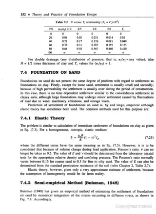
Pore· pressure corrcc.tion factor. J1 = 0. 7
(refer Fig. 7.4)
p, = 0.7 x 62 = 43.4 mm
Final
se t~ emen t
= 4.8 + 43.4
= 48.2 mm
From Eq. (7 .17),
I - 2v
K' = I [ I + !J(l + !J)(3A
Substituting v = 0.3 and A = 0.7,
K' _ I _ [
I - 2 x 0.3
]
I + 0.3(1.3)(3 x 0. 7 - I)
= 0 .84
From Fig. 7.7, for undisturbed Calcutta soil
.l. = 0.6
{f, = 0.6 x 43.4 = 26 mm
PJ = 4.8 + 26 = 30.8 mm
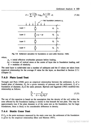
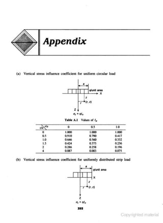
Example 7.2
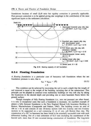
A raft foundation. 8 m x 12m in plan is to be placed 2 m below G. L. in the subsoil shown in
Fig. 7 . 10. The net foundation pressure is 50 kNfm2• Calculate the total settlement of the
foundation
Raft foundation
8 m x 12 m
0
50 kNtm'
II I II II
--
-2m
~~5Am
m
/
/
- Sm
f
f
I
I
I
f
'
/
E
:
Fig. 7.10
I Fwm desiccated silty clay
y • 18 kNtm3
' C11 • 40 kN!h'Y
c,11 + eo= o.06
'-
+a
I
I
I
I
II Soft ()(ganlc silty clay
r = 11 kNim'
~ = 25 kNii
c,J1 . .. = 0 .12
m
'
Raft foundation on day.
Copyrighted material

177. Set1lement Analysis • 157
Take influence zone extending to twice the width of foundation. thai is, 16 m below
foundation. Neglect the effect of settlement due to sand layer.
Solution
(a) Immediate senlement
P; =
For the given problem,
q. =50 kN/m2
8=8m
v = 0.5
l p (for UB = 12/8
for.
= 1.5) = 1.36 (refer Table 7.1)
£ 1 = 600 x 40
Stratum 1:
Stratum II:
= 24.000 kN/m2
£ 1 = 600 x 25 = 15,000 kN/m2
Weighted average. E
24,000
X
3 + 15, 000
13
X
10
= 17,000 kN/m2
...
50
X
8
P; = 17,000
X
0.75
X
1.36
= 0.024 m = 24 mm
Depth correction = 1.0
Rigidity correction = 0.8 (Considering ran with interconnected beams providing rigidily to
the foundation)
(p;)""'
= 0.8 x 24 = 19 mm
(b) Consolidntiotr s~ulemelrl
p.., =
I
C,
!:.! A~
P•c.:,
- - H Iog- +_;: p
l +tto
p.,
At A. p. = 18 x 2 + 8 x 1.5 = 48 kN/m2
Ap
= 0.82 x 50 = 41 kN/m 2
At 8, p 0 = 18 x 2 + 8 x 3 + 7 x 5 = 95 kN/m1
Ap
= 0.42 x 50 = 21 kN/m2
PO«l = 0.06 X 3
X
log
48 + 41
95 + 2 1
+ 0. 12 x 10 log
48
95
= 0.048 + 0.104
= 0.152 m = 152 mm
Copyrighted material

178. 158. • Theory and Practice of Foundation Design
Using. depth correction = 1.0
Rigidity correction = 0.8
:.
(p.,..),., = 0.8 x 152 = 121 mm
Skempto11 and Bjerrunr method
p, = p(p.,..)""'
Take J1 = 0.8 (settlement being predominantly in soft normally consolidated soil of
stratum II)
:. p, = 0.8 x 121 = 97 mm
:. Pt = 19 + 97 = 116 mm
StrHs-poth method
p', = ).p,
from Eq. (7.17)
I - [I + 7](1 - t7~~3A - I)]
](' =
Substituting v = 0.3 and A = 0.8
K' _ I [
I - 2 x 0.3
]
- I + 0.3(1.3)(3 X 0.8 - I)
= 0.84
From Fig. 7.7,
). = 0.6
.. Jf,=0.6x97=58mm
Pt = 19 + 58 = 77 mm
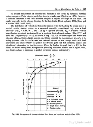
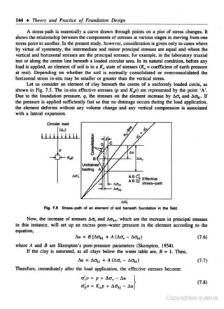
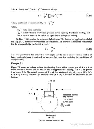
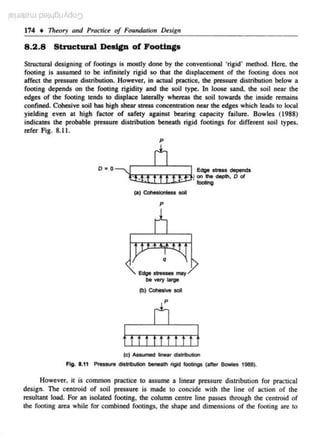
Eumple 7.3
A S m x S m foundation is placed I m below G. L. in the stratified sandy deposit as
depicted in Fig. 7.11. Calculate the settlement of the foundation.
1600kN
1m
5m
i
'I'
I
I,
•m
--
Medii.ITI sane~
r• 18~
N = 20
= 8000 kNim'
'
+
' c..
I
1
5m
I
+.
/
,,
I
' Medium sand
I
I
r=
19 kNim~
N • '2!5
clll:f = 1
o.ooo kNfml
Medium sand
r• 20 kNim3
N • 30
c.,= 12.ooo kNim'
Flg. 1.11 FCIUI'Iaation on sand.
Copyrighted material

179. Sttrlemeru Analysb
t
159
S<Jiution
Net foundation pressure.
q. =
1600
4 x 4
= 100 kN/m2
(a) Elastic tlreory
8= q,B (I - v 1 )1
E
P
Also.
q11 = 100 k:N/m2
8=4m
v = 0.3 (assumed)
lp
E
= 1.12
= C1 +
C1N (Take average N value of the two layers having almost equal depth
wilhin the influence zone)
: 39 + 4.5
X
22.5
= 140 kg!cm2
= 14,000 kN/m2
.
..
4
X
14,000
= 0.029 m
8 : IOO
=29
For,
:.
X
0.91
X
1.12
mm
L = I and !!J.. = 0.25,
8
8
(8)""' = 0.97 x 29 = 28 mm
Depth correction, a = 0 .97
(b) 8uisman (1948) met/rod
Consider two layers within the influence zone
<-
""
" - £....
At A,
Po
=I
2.3p. I
Po + bp d
E og,.
•
Po
x 18 + 2..5 X 8 = 38 kN/m2
bp = O.S6 x 100 = 56 kNim2
E1 = 39 + 4..5
At 8,
X
20 = 129 kgtcm' = 12,900 kNim2
Po = I X 18 + 5.0 X 8 + 2.5 X 9 = 80.5 kNJm'
Ap = 0.11 x 100 = II kNJm'
E 1 = 39 + 4.5 x 25
.
..
= 151.5 kg!cm2 = 15.150 kNim2
_ 2.3 X 38 S I
38 + 56
2.3 X 80.5
I
80.5 + 11
8 - 12,900 x 0810 38
5 0810 80.5
+ 15,150 x
= 0.013 + 0.0034 = 0.0164 m = 16.4 mm
Copyrighted material

180. 160 • Theory aud Practice of Foundation Design
Depth correction = 0.97
:.
(o)..,.. = 0.97 x 16.4 = 16 mm
(c) Beer a11d M arte11s (1957)
•
"=
2.3H
----c- 1og,o
p0 + Ap
P.
lAyer I:
II = 5 m; Po = 38 kN/m2; Ap = 56 kN/m2
..
1..:.:
C = - 9 c::l•O!.•
= 1.9 X 8000 =400
38
lAyer 2:
H = 5 m; Po = 80.5 kN/m2; Ap = II kN/m1
c=
•
u
1.9
10,000 : 236
80.5
X
2.3
= 400
X
51 0810
38 + 56
2.3
38
+ 236
80.5 + II
Slog,O 80.5
X
= 0.012 + 0.0027 = 0.0147 m = 14.7 mm
Depth correction = 0.94
:.
(0)""' = 14.7
X
0.94
e
14 mm
Examp1o 7.4
The "'suits of a plate load test on a sandy stratum arc shown in Fig. 7.12. The size of the
plate used is 30 em x 30 em. Determine the size of a square footing for a column carrying
a load of 1800 kN with a muimum permissible settlement of 50 mm.
0
,
0
--
L.oadllnll area (KN!m2)
200 •
400
..
r--- .....
600
""'""'
800
1
60
10
Fig. 7.12 Plate load test data.
Copyrighted material

181. Settlement A11alysis •
161
Solution
The problem has to be solved by trial and error.
First trial
Size of footing = 3 m x 3 m
q. = 180019 = 200 kN/m2
sf
From Eq. (7.27)
s,
4
=
(I+
.. s,
~;)'
~(~ + Ee.r
D1
= 4
= 50(~ +~r
4
3000
=IS mm
Allowable pressure (From curve) = 440 kN/m2
Second trial
Size of footing = 2 m x 2 m
q. =
Again,
s, ~
SO
4
(I +
= 16.S
1800
= 4SO kN/m2
2x2
300 )'
2000
mm
Allowable pressure = 480 kN/m2
Bjenum. L. (1964), Reilujo11 Mellom Malte og Beregnede Set1ti11ger a v Byggverk po Leire
og Sond, N.O.F. Foredrage.t, 1964. Norwegian Geotechnical Institute, Oslo 92 pp.
Bjerrum L. ( 1963), Discussion on Section 6. European Confeunet S.M.F.E., Wiesbaden,
Vol. 2, pp. 135-137.
Butler, F.O. (1974), General Report and State·oftht-Arr Rt•iew, Session 3: Heavily
Overconsolidated Clays, Proceedings of Conference on Settlement of Structures.
Cambridge.
Copyrighted material

182. 162 • Th.eory and
Practk~
of Foundation
tsign
Oas. S.C. (1975). Predicted and Mea.sured Va es of Stress and Displacem~nts Downloadi,g
and Constructiotr under Circular Fof ings Rtsting on Saturated Clay Medium,
Pll.D. Thesis, Iadavpur University, Calc ta.
Das. S.C. and N.N. Som (1976). Smlemm of Footings on Soft Clay, Proc. Symp. on
Foundations and Excavation in Weak S<fl, Calcutta, Vol. I.
Davis. E.H. and H.G. Poulos (1968). The usl of Elastic Theory for Settlement Prediction
under Three-dimensional Conditions. Ge4teclmique, Vol. 18.
rie
Beer, E.E. (1965), Bearing Capacity andJsmlemtllt of Shallow Foundations on Smtd,
Proc. Symp:>sium on Bearing Capacity atil Settlement of Foundations, Duke University,
pp. 15-33.
De Beer. E. and A. Martens (1957), Meth ' of Computation of an Upper Limit for the
Influence of Heterogeneity of Sand l.Ayet s in Senlement of Bridges, 4th I.C.S.M.F.E.,
London, Vol. I. pp. 275-281.
J
Fox. E.N. (1948), The Mean Elastic Senlemen of Unifonnly Loaded Area at a Depth INlow
Ground Surface. 2nd l.C.S.M.F.E.. Rottdidam. Vol. I. p. 129.
Guha, S. (1979). Effect of Initio! and Incremental Strain Ratios or Drained Defonnotion of
Calcutta Soil. MCE Thesis, Iadavpur u.Jversity, Calcutta.
Ladd, C.C. (1969), The Prediction of in-situ S ss-$tmin Behaviour of Soft Saturated Clays
during Undrained Shear, Bolkesj • Sym sium on Shear Strength and Consolidation of
Normally Consolidated Clays. Norwegia Gwtechnical Institute. Oslo, pp.l4-19.
Lambe. T.W. (1964). Methods of Estimatin Settlement, Joumol of Soil M<ehanics and
Foundation DiviJion, A.S.C.E.. 90, No. SMS. pp. 43-67.
Raymond, G.P., D.L. Townsend, and MJ. Lo!asek (1971). Tbe Effe<:t of Sampling on the
Undrained Soil Properties of a Leda
Canadian Geotechnical Journal. Vol. 8,
pp. 546-557.
s ·l,
y
Simons, N.E. (1957), Stttltmtnt Studits on
London. Vol. I, pp. 431-436.
o Structures in Norway. 4th I.C.S.M.F.E.,
Simons. N.E. and N.N. Som ( 1970), Stttlt ent of Structures on Clay with Particular
Emphasis on London Clay, Construction dustry Research and Information Association
Report 22, p. 51.
Skempton. A.W. (1954), The Pore-pressure
fficients A and B. Gtotechnique. Vol. 4,
pp. 143-147.
Skempton. A.W .. R.B. Peck, and D.H. Me onald ( 1955), Stttlemtnt Analyses of Six
Structures in Clticogo and l.Andon. Proc I.C.E.. Part I, Vol. 4, No. 4, p. 525.
Skempton. A.W. and L. Bjerrum (1957), A ontribution to the Settlement Analysis of
Foundations on Clay. Gtotechniqut, Vol. 7, No. 4, pp. 168-178.
Som, N.N. (1968). Tl1e Effect of Streu Pat 011 tire DeformaJ•'on and Consolidation of
London Clay, Ph.D. Thesis, University o London.
Copyrighted material

183. Senlement Analys;s •
163
Som, N.N. ( 1975), Regional Deposits: Co,tribution for Panel Discusslon, Proc. 5th Asian
Regional Conf. in SMFE, Vol. 2, p. 20.
Taylor. D.W. (1948), Fundam•ntals of Soil M.chuuics, John Wiley and Sons, Inc,
New York.
Terz.aghi, K. (1943).
n~<omical
Soil Multanics , Jnhn Wiley and Sons Ltd.. p. 510.
Terzaghi. K. and R.B. Peck (1948), Soil Muhanics in Etrginuritrg Practia, 1st ed ..
Wiley. New York.
Copyrighted material

184. Footings and Raft
Design
8 . 1 INTRODUCTION
Footings and rafts are the common shallow foundations wherein the subsoil immediately
beneath the ground s urface is required to suppon the foundation. load. The superstructure
load from a building is transmitted to the ground through columns and load·bearing walls
and sujtable structural members are to be provided to transfer the load into the s ubsoil. These
struc.tural members which are placed at some depth beneath the ground surface serve to
;spread' tbe load from high stress intensity of the superstiUcture malerial (concrete. steel, or
brick) to the low allowable stres'""' in the soil mass.
The different types footings and rafts have been illustrated in Chapter 4. They are
generally made of reinforoed concrete. The reinforoements are provided to resist the bending
moment on lhe footing caused by the upward soiJ reaction either in one direction as in the
case of strip footings or in two directions as in case of isolated or combined footings. refer
Fig. 8.1. The section of the footings may be sloped to economize on the volume of concrete.
Heavily loaded structural steel columns are sometimes provided with grillage foundations.
. . ...
I
-+-+
r_,+-+C.J
(a) ISOlate<! tooting
~
~
~
I
-tt:8:+- ---+-HL.J
4
(bJ Sll1p looting
(e)
Com- looting
FIQ. 1.1 lsotatecl. slrlp. anc:s combined tooc:lngs.
16.
Copyrighted material

185. F(J()tiugs and Raft Ol!sigu • 165
The design of sha.llow foundation involves detennination of:
I . depth of foundation,
2 . allowable bearing pressure and size of foundation. and
3. settlement of the foundation.
8 .2
8 .2 .1
DESIGN OF FOOTINGS
Depth of Footing
The minimum depth at which a foundation should be placed depends on the soil profile,
structural requirement. ground water condition. and so on. The following factors should
generally be taken into consideration in determining the depth of foundations.
(a) Depth of top soil, rubbish fill, if any.
(b) Depth of poor surface deposit such as peat, muck, or sanitary land fill.
(c) Location of ground water table and its seasonal fluctuation.
(d) Depth to poor or better underlying stntta.
(e) Depth of adjacent footings if any.
lf the subsoil near the ground surface consists of a heterogeneous fill of uncenain
propenies or compressible soi.l like peat, muck etc. the foundation should. preferably. be
taken below the fill. Figure 8.2 is a clear repn:sentation of the same. It is also desirable that
the foundation be taken beJow the zone of seasonaJ fluctuation of water tabJe where the soil
is not subjected to seasonaJ volume changes due to alternate wetting and drying. For this, the
foundation is generally placed l - 2 m below ground surface. However, if the water table
fluctuates over a great depth, it may not be economical to take the foundation to the desired
level. The foundation may then be placed at some convenient depth and the design done for
the highest position of the water table. The depth of foundation is also influenced by the
location of underground facilities below the building. ln case where a stiff clay is underlain
by n softer material, the foundation should be placed as high above as possible so that the
pn:ssure bulb may be restricted within the stiff c lay.
Pea~
Muck etc.
'
I
'
~Finn soil
,
I
Soft soil
Fig . 8.2 Depth of footing.
Copyrighted material

186. 166 • 111eory otUI Practice of Foundarion Design
In sandy strata, if there is marked increase in density of sand with increasing depth, it may
be tempting to take the foundation deeper than normal in order to take advantage of the
higher bearing capacity. This proc--edure may not be economical if it involves deep excavation
below the water table involving large scale dewatering. Further. there may be problems with
the stability of side s lopes and adjacent structures.
8 .2 .2 Allowable BeariDg Capacity
The net allowable bearing pressure on footings should be detennined from considerations of
bearing capacity and settlement. so as to satisfy the requined design criteria. The methods of
bearing capacity and settlement analysis have already been described in Chapters 6 and 7.
First. it is necessary to establish the depth of soil which is significantly affected by the
foundation loading. As a general rule. this depth may be taken as twice the width of footing.
All the strata contained within the significant depth of soil are to be considered in the design.
The reJevant soiJ parameters for each stratum need co be evaluated from appropriate soil tests.
Figure 8.3 shows rypical examples of the s~g.ni fic.ant depth of soil for different size of footing.
rl
- --
0
E
n
•
~ ~ .sm..I'
/
I
I
I
, ....
,
3.Sm
I I<
-+1',
I
~U~
......_ftueoce
In
--""zone
-
0
I
I
I
I
Ooplh
Stratum I
A rm desiccated
I
I
I
,
'1 ,._
·
silty day
IE
' ' f--
- ---- - ,--- --- ----~-
Pressure
lnftuence
zone
f',
I
Stratum II
Soft Otglnle
I
I
8illy ClOy
' ' ' __ _........
I
I
I
/
/
/
-8 m
- 8m
Stratum
tn:
Slitf clay
Fig. 1.3 Significant depth of soli below founctftlon (preUI.Q bUlb).
Keeping under consideration shear failure of the soiJ, lbe ullimate bearing capacity of
footings on different typeS of soil may be obtained as follows:
(a) Coh.siv• soil (' ; 0)
q, (n) = c. N,
(8. 1)
where, c,. = undrained shear strength of the soil and
N~ = bearing capacity facror
=
51 o.~8)(' 02:1)
(
+
+
(8 and L are the width and length of footi ng)
Copyrighted material

187. Footings and Raft Design • 167
The shear strength of the soil within the failure tone below the footing. that is. within
a depth approximately equal to the width of footing. should be used in design. In view of
the natural variation of soil properties at a building site. there is usually a wide spectrum
of test results and the designer is required to exercise his judgment in selecting the
design shear strength. For a stratified deposit. a weighted average shear strength may be
used in desi.g.n. However. it is to be realized that if the major portion of the failure surface
is coatained in stratum I , the bearing capacity of the foundation would be detennined
primariiJ by the undrained shear s..-ngth of stratum I. Figu"" 8.4 depicts a failure surface·in
stpotifi<:d soil.
- - - Failure sulflce In _,m I
- - - -
Fallure
surface In sntum u
Fig. lA Failure surface in stratified soil.
(b) Granular soils (c
= 0)
q•• (n) = q(N, - I ) + 0.5sy'BN1
(8.2)
where.
q ; effective surcharge at the foundation level,
r' = effective unit weight of the soil below the foundation.
8 = width of foundation,
N" N1 = bearing capacity factors (see Chapter 6). and
s = shape factor (0.5-1.0).
(c) Soil lrnvlng both c and ;
The general bearing capacity equation given in I.S. 6403-1981 may be used to determine
the bearing capacity of soils having both c and ;•.
(8.3)
The shape, depth. and inclination factors to be used in Eq. (8.3) are given in Table 8.1. The
effect of water level should be taken into account in determining the values of q and y '.
N(', N., and Nr are functions of the angle of shearing resistance of the soil obtained from
laboratory tests or from empirical c.orrelation with the field standard penetration resistance, N
(for details. sec Chapter 6).
Copyrighted material

188. 168 • 17Jeory and Pmctice of Foundah'on Design
Ta ble 8.1 Shape. depth. and inelinarion factors as per IS:6403-J98l
Far:sors
Slwp~ facto rs
Valla!
~)
( J + 0.2
for rectangle
1.3 for square and cirele
'•
(1
+ 0.2
.Z,)
for reelan&)t
1.2 Cor square aod circle
,,
(I - 0.4~) for rtetangle
0.8 for squ:are '"d 0.6 for circle
d~plh
factors
d,
1
+0.2~ •an(4S'+ i)
I + 0.1
1 for
~
~tan( 45° +
t}
for
~ > JO•
< 10•
Jndlnalion foctor:r
(I - ~)
,,
·(1 ain degrttS
-:)
from the ultimate bearing capacity. the net allowable bearing capacity of a foo ting,
QaJJ(n), is obtained as
qau(n) -
q,. (n)
F
where. F
= factor of safety
8 .2 .3
(8.4)
Effect of Ground Water Table
(normally 2.5-3.0).
The effect of ground water mble on the bearing capacity of shallow foundations has been
discussed in Chapter 6.
The effective s urcharge. q at the foundation level is to be determined by using the
appropriate density (bulk or submerged) of the soil above the founda tion level. For ground
woter table coinciding with the ground surface. submerged density is to be used for the full
depth of soil above founda tion level. r' on the Olher hand, is lhe effective unil weight of the
soil below the fou ndation. As the failure zone extends to a depth approximately equal to the
width or footi ng, the effective unit weight within this zone is to be considered. For the water
~able at or above the foundation level. submerged density should be used while fo r the water
Copyrighted material

189. Footi11gs and Raft Design • 169
table at a depth greater than 8 below the footing. bulk density is to be used. For ;l!Y
intermediate position of the water lJible, the effective unit weight may be obtained, ttMn
interpolation between rand y', as shown in Fig. 8.5.
1
<D
o,
® •
q
Ui
lo- B
iLU
r'
--oj
B
•
Fig. 8.5 Elloct ol ,..,., table on bearing capacity.
8.2.4 Settlement
Trial dimensions are chosen to accommodate the required footi ng as given by the allowable
bearing capacity of the footing. The settlement of the footing is then estimated for the actual
net foundation pressure, q,. given by,
q, =
Q
-:---~':--,-­
(8.5)
q,B (I - v 2 ) I
(8.6)
Area of footing
where Q = net load on the footing.
For footings on clay,
(a) Immediate senlement
E
where,
•
q,. = net foundation pressure.
B = width or foundation,
E = modulus of elasticity of the soil within the zone of influence,
lp = influence coefficient. and
v :: Poisson's ratio.
(b) Consolidation
senle~nt
P~
where. C, /(1
H =
p0 =
tlp =
J1 =
= J1"" J C, <o H log P. + l!.p
L... +
Pu
(8.7)
+ to) = compressibility index of the clay.
thickness of compressible stratum.
in~situ
effective overburden pressure at centre of stratum,
increase of venical stress at the centre of stratum due to the foundation
loading, and
pore-pressure correction fac tor.
Copyrighted material

190. 170
t
Th~ory
and Practice of Foundation Design
If the coefficient of volume compressibiljcy. m. is used. the consolidation senlement is given by
(8.8)
Tile detailed procedures for settlement calculation are given in Chapter 7.
(c) Total settlement
(8.9)
The depth correction and rigidity correction should be applied wherever applicable. If the
settlernen~ as estimated from the above, is within the permissible limits, the foundation may
be considered final. If not, the calculation should be repeated with revised footing dimensions
until the sen1emcnc criteria are satisfied.
Although settlement of footings on sand is generally small, unless the sand is loose
(N < 10)-it may be necessary to check the anticipated set~ement to see if it exceeds the
tolerable limits. As has been discussed in Chapter 7, the semi-empirical methods would be
preferable to any theoretical analysis (See subsection 7.4.2).
Some complications arise when two different kinds of soil (s.ay. sand and clay or vice
versa) fall within the inOuence zone. ln such cases, the set~ernent of the sand layer can be
obtained separately and added to the settlement caused by the clay strata. There is usually no
problem in determining the consolidation settlement of the relevant depth of clay strata using
appropriate expressions. However, if the clay stratum is of lesser thickness than the depth of
pressure bulb, the immediate settlement due to the clay layer may be overestimated. The
designer may apply his j udgment in evaluating the immediate settlement of individual stratum
giving due importance to the relative contribution of each stratum.
8 .2 .5 Dimensioning Footing Foundations
(a) bolated foottqo
As a general rule, square footings give the most economic stroctural desi,g.n for a given
column load. In case of space restriction, it may be necessary to go for rectangular footings.
as shown in Fig. 8.6.
rr:=~;===-::-==~-;:==:-j
:r:r.~ ::
rn : : r:.Gd ! ; P'7l :
f'7A
.~
~
•
l ........•• •. _________ ,}. ,. ...........,)• , r.Gf , l
. . .....
I :·---- ;
I •
'
r•·••· j
)..______
1:
'
: .....
.... :
:
............: :
ll~ !
J
:
:
~-----*
Square
: ~ :
,-----· I
:
!I
: ~! : ~ : 1
Rectangular
. :: 1
~--·--'
1
I -----, _ ./, __ _______, ------. I
_______
: f1'7.:1
r7l.
: :
m
: :
l ........: : ....... ..... __________:: m:. l
: ~ : ..
:
~
: :
r.Gd
w
....... .J..J
l
-------, ----
Property line
Fig. 8.6 Square and rectangutar footings.
Copyrighted material

191. Footings and Roft Design • 171
(b) Combined foottngo
Two or more columns in a building frame may be supported on a single footing. eithe.r
recmngular or trapezoidal when isolated footings tend to overlap or extend beyond the prope~~
1
line. If the allowable bearing pres..'ure is known, the sjz.e of lhe footing may be determined for
a permissible settlement. In onder to get uniform bearing pressure. the footing should be so
proponioned that the resultant column loads pass through the centroid of the footing area.
Figure 8.7 shows typical combined footings of rccmngular and trapezoidal shape.
Cont>lned
(c) Strip footlngo
Strip footings arc provided below load bearing walls or a row or columns in building rrarne.
Even if the column loads vary a little. the longitudinal extent of the footing normally ensures
a uniformly distributed load below the footing. A pedestal may be provided if a singly
reinforced scrip fooling along lht width is desired below closely spaced columns. This is
depicted in Fig. 8.8.
r----------- ,
::
:v
I
::
I
L_..!
I
•
Strip footing
AtJ ->WA -----,---
, .-.
I
I
Load bearing wall
I
I
L - .-.
-
Brick wall
--.
I
I
I
I
I
I
__ I
••••
Section AA
Fig. 8.8 Strip footings.
Copyrighted material

192. 172 +
8 .2 .6
17~tory
and Practic. of FoundtJJU'" Design
tDterf~ce
effect
When a number of closely spaced colulllll$ ate required to be supported on ioolated footings,
the pressure bulbs under individual footings tend to overlap, as shown in Fig. 8.9. According
to Boussinesq stress analysis, the pressure bulb below a footing extends to a distance of 812
on either side of the footing (where B is the width of footing). If two adjacent footings come
to within a distance B from each other, the pressure bulbs overlap and the soil below the
depth. D behaves as if it is loaded by a combined footing. The settlement or the footing as
determined for an isolated foundation is no longer valid. The effect or superposition or
stresses should be taken into account in estimating the settlement. Appropriate stress analysis
for adjacent footings, taking into consideration the interfen:oce effec~ may be done to obtain
the soil stresses for calculation of settlement.
0
Stress intloenoe zone
.J
IC
I
6 tij 6·C:'": ...
tl+-s-ol,
f
I
~I{
tl•- s-..1,
,jo
I
1
' ... __ ..
'
"
I
/
I
I
'
I
' ... __ ... ,
'
"
~0.1q stress contour
I
I
In order to ensure the behaviour of footings as isolated footings, the spacing between
adjacent footings should not be less than the width of footing. If the footing size varies, the
spacing between footings should be equal to the width or the larger footing.
8.2.7 Destp for Equal Settlement
Isolated footings in a building frame tend to settle individually and the columns undergo
differential settlement depending on the loading and subsoil condition. Attempts should be
made either to design the footings in such a way that the differential settlement and hence. the
angular distortion between adjacent footings are kept within pennissib1e limits or
interconnected beams may be provided at the foundation )eve) to increa..(iC the rigidity Of the
foundation.
Copyrighted material

193. Footings and Raft Design • 173
The basic factors which affect the settlement of footings on a given soil are the
intensity of loading and the size of the loaded area. The settlement increases in almost direct
proportion to these parameters. It is a common experience that even though the foundation
pressure is the same under all footings. a bowl shaped defonnation trough is obtained with
greater settlement at the centre than along the edges of the building mainly due to greater
load in the central columns and the overlapping of stresses from adjacent footi ngs. Hence. to
produce uniform settlement, it may be necessary to adjust the pressure with size of footing,
that is, to impose greater pressure under smaller footings than under larger ones and also to
use larger pressure under the footings along the edge of the building. The principle was
utilized in the CB 1 Esplanada Building, Sao Paulo which was founded on moderately
c.ompact fine to medium sand. A pressure of 550 kN/m2 was used under the outer footings
and 400 kN/m2 under the inner footings. with the result that the maximum differential
settlement did not exceed 8 mm (Skemp<on, 1955). So. the bearing pressure of footings in a
building frame may be varied though it is always kept within the safe bearing capacity so as
to have the maximum and differential settlement within permissible limits. This may require
a number of trials before the final design is arrived at. A simple calculation for achieving
unifonn settlement of adjacent footings is shown in Example 8.4.
A satisfactory method of reducing the differential settlement of footings in a building
frame is to provide interconnected beams between columns at the foundation level. A framed
structure is tied laterally. from fin;t noor onwards, by beams and s labs but no such
connection is generally provided at the foundation level. Consequently, the individual
footings can settle differentially. Providing interconnected beams increases the rigidity of the
foundarion and differential senlement is substantia1ly reduced. An approximate way of
analysis would be to estimate the settlement of individual footings as isolated/strip footings
and then to design interconnected beams to resist the bending moment at the joints due to the
differential settlemenL For more accurate design. theoretical analysis of the building frame
may be done with predetermined sections of the interconnected beams and footings.
Figure 8. 10 shows a typical strip foundation with interconnected beams.
D D ~~;AS:,-~I
D Ej
tJ D d b
I
I
I
Sedion AA
I
.JA
Strip
•
•
I
I
•-""
lnterc:onnecled
beam
I
_;r
v
I
•
I
j_p
•
I
I
~
ww
I
I
I
I
Slrip
Fig. 1.10 Strfs) tooU.ngs with Interconnected beams.
Copyrighted material

194. 174
t
D~.sign
T!Jtory and Pracrict of Foundatio
8 .2.8 Structural Dealgn of F
StruciUral designing of footings is mostly do by the conventional 'rigid' method. Hert:, the
footing is assumed to be infinitely rigid so that the displacement of the footing does not
affect the pressure distribution. However. in tual practice, the pressure distribution below a
footing depends on the footing rigidity and the soil type. In loose sand, the soil near the
y whereas the soil towards the inside remains
edges of the footing tends to displace lat
confined. Cohesive soil has high shear stress c;pncentration near the edges which leads to local
yielding even at high factor of safety ag&inst bearing capacity failure. Bowles ( 1988)
indicates the probable pressure djstribution r neath rigid footings for different soil types.
refer Fig. 8. II.
~
I
0•0
(a) Coh<+
lltess soil
q
Edge
be
(b)
s may
velY large
l ive soli
p
(c) As&umed linear distribution
Flg. 8.11 Pressure disUibulion benet
rigid fooelngs (after Bowles 1988).
However, it is common practice to assui a linear pressure distribution for practical
to concidc with the line of action of the
design. The centroid of soil pressure is rna
resultant load. For an isolated footing, the col n centre line passes through the centroid of
l
the footing area while for combined footings, 1 e shape and dimensions of the footing are to
Copyrighted material

195. Footings and Raft Design • 175
be determined 10 achieve this condition. Once 1he pressure distribution has been obtained for
the chosen geomerry of the footing, the stnJctural design of the footing is made to resist the
shear forces and bending movement for the appropriate suppOn conditions. For isolated
foolings. the cantilever bending moment at the column face will normally determine the
amount of reinforcement to be provided. In case of combined footings, the design is a simply
supported beam with overhang on both sides whiJe a strip footing is designed as a continuous
beam with support at the column locations.
8 .3
DESIGN OF RAFT FOUNDATION
A raft foundation usually covers the entire area of the building, thereby distributing the total
load to a larger area than a footing foundation and reduces the bearing pressure to a
minimum. The choice between a raft and a footing foundation depends on the soil properties
and the weight of the building. If a preliminary design wilh footing foundations reveals that
the sum of the footing areas required to s uppon the. structure exceeds 60% of the total
building area, a raft foundation covering the entire area of the building should be preferred.
Moreover, where the soil properties vary largely throughout the site, the amount of
differential settlement may be excessive for a footing foundation, but with a raft foundation
the effect of weak zones scattered at random tend to even out. Therefore, the settlement
pattern is Jess erratic and the differential settlement is also reduced considerably. Also. a raft
fou ndation provides increased rigidity which reduces the differential movement of the
superstructure.
8.3. 1 Types of Raft Foundation
Two types of raft foundation arc in common use which fonn a subject mauer of discussion
in this subsection.
(a ) Conventioaal raft
In conventional raft (refer Chapter 4. Fig. 4.7) foundation, a flat concrete slab of uniform
thickness covering the entire area of a building is placed at some deplh beneath the ground
surface and the columns are built directly on the raft. Then backfilling is done upto the
ground level. This is followed by further fi lling, called the plinth filling, on which the
ground floor slab is placed. The ground floor load, therefore, goes to the raft by direct
bearing through the plinth and backfill.
Figure 8.12 shows some typical rafl foundalions. The columns may be placed directly
on the s lab or 1he slab may be thickened under large column loads 10 give sufficient s1rength
agains l shear and support moment. Rigidity of the raft foundation may be increased by
cellular construccion or rigid beam and s lab construction. Figure 8.13 shows a simple raft
foundation for the fourteen-storeyed block of tlars at Golden Lane, London (Skemplon,
1955).
Copyrighted material

196. 176 • Theory and Practice of Foundation Design
A
t.
LlJJJ, J:WJJ ~
.---,.•
•
•
•
•
•
•
•
B- B
A- A
E-E
• • •A
--,. -· .,. ---,
• •
® ® ® ®
• • •
• • •
® ® ® ®
•' ' ' •'
B E '
•'
':.. .... -·~ .... -·:..- ....·:..
''
''
j
t
® ® ® ®
''
--... E
·---.·---.·---.·.... J
'
•'
.. ..
... .. .. . ---.
•' .. .. .
'
-:-~ - -, -:-~~~.
- -
';:.-.-. :------,
'' ' '
'' '' ''
''
.... ..•:..- ....''•:.. __ _:_ __ .
·
'
-
Fig. 8.12 Typical raft foundations.
~
£
~
c
~
l
Average gross
pressure under
raft: 190 kNim2
Clay
•.2m
II
- L
. 13.4m
-~ . 1:!i/E
1:;;
London clay
Fi.g. 8.13 Raft foundation for Golden Lane ftats. LondOn ($kempton, 1955).
Copyrighted material

197. _ _ _ _ _ _ _ _ _ _ _:..;ootings nnd Raft Design • 177
F.
(b)
Buoyaac:y raft (oUDdatiOD
Vith 1he incru.5Cd number of tall buildings now being buill for vanous commerei:d and
residential putpOSeS, rafl foundauons bavc been CO'Coiendy combu!Cd Wllh !he: principle of
fkxlllluon. Buoyancy rafts (refer Chopccr 4, Fig. 4 .8), wnh or without ba!cmcnt. an: placed at
some depth beneath the around surface. but no backfilling is done on the raft. A struc1ural slab
is made. usually a linlc above the ground level to serve as the ground Roor of !he: building. The
space between the ground floor slab and the raft is kept void such that the net foundU~ion
pressure gets rtduced and remains within the permissible bearing pressure on the foundation.
That
q.., = q,....- yD1
is.
(8.10)
< q,.t{rr)
where, qlrot• • gross roundmion pressure.
yD1 • lOCal overburden pressure at the foundation level, and
q,11{n) " net pennissible bearing prcssun:.
SPace
When a buoyancy ron has sufficient bead room below !he: around Roor •lab. the
may be utilized u • basement Roor below the ground. Although a ba!cment is. in effect. a
buoyancy raft. it is not necessarily designed for the purpose. The main function of a
basement is to provide addlt.lonaJ floor space in the buildlna and the fact that it n:duees !he:
net bearina pressure may be quite incidenllll. A buoyancy raft may, ho"'-ever, be designed
solely for the purpose of providing suppon to !he: slnl<:ture and to reduce the ta<al and
differential settlements within permissible limits.
8.3.2
Beartn& Capacity
The mechanism or benring capacity failure of raft foundation is similar co that of footings.
except that the former involves 11 much bigger and deeper zone or foilure.
The net ulcimnte bearing capacity of a roft foundation Qu1
,(n) is. therefore~ given by the
same expressions ns or Footings, as illustrated by Eqs. (8. 1H8.3). However. rnn foundmions
being much larger than Footings. the pressure bulb ns well as the failure surface extend to
considernble depth below the foundation. A typical raft foundation on nonnnl Cnleuun soil is
shown in FiJ. S. J4. As 1een. more than one s-rnnum with different shear paramete.rs are
involved. A weighted a•erage strength or the strength or the most predomjnant strarum
within the failure zor.e may be used to detennine the bearing capacity.
8 .3 .3 Settlement
The immedtate and eonsoltdauon settlements of raft foundations on clay are obtamed an the
same manner IS for fOO<on&S. see Eqs. {8S) and {8.6). The <Ompt'eSSIOD Of all !he: stralll within
!he: signifocont depth below !he: foundation are to be calculated separately and !he: summation of
all these seulements woll give the ta<al settlement of the foundation. Use or Eq. (8.6) to
calculate the immeduue sculement presumes that the subsoil behaves as homogeneous. isotropic.
e.lastic medium. In case of non ·homogeneouslstr.ttified deposit. this is somewhat approximate.
but is often accepted for practical purposes. More rigorous analysis. taking into account the
variation of subsoil properties. can also be done. Depth correction Is no1 slanificant for raft
t u, righted materio1l

198. 178 • Theory and Pmclice of Foundation Design
foundat ions because of small DJ'B ratio but rigidity correc1ion is generally applicable.
Pore-pressure correction is to be applied giving due weightage to the contribution of the most
significant layers in the settlement calculation.
~~'-i~~~~'~;;;t;;:;j;;;,;J;;:~t~lt":.;,~o..;:;!;.cca!~ btcw.nlsh gtoy silty day:
. ,
'..::
•
3 _ ''-::----r-'--'"'-----;,£----',----c::,.•_,,:..!IO~kNirn', Cc/(1 +eo) = 0.05
' ,
I
_, "
'
'
I
I
'I
:~....
I
'
....... ___ ,. "
...
',
... ... ___ ....... ,.. ' ~
I
"
/
.;
I
1
II Greyldartt grey Of'gank:: sil ty clay
J
with decomposed wood:
r
c., • 25 kNim2, C(l/(1 +eo) • 0.15
l
t
1 4-----~~----------------------+~~~~
· Ill Firm bluish
1
,
18 _____
I
.:<:-·.::
•..:60=-:kNim2, c , t(1 +eo)= 0.10
rv Brownish/greyish brown sa.ncty
_,t-- - - - - - -- --_,,:. 7
'
/_
,
1
',
/
grey silty clay with
caJcareous nodUles:
slit: N
=12
~ ----------~------------~---------brown
' ....... ,
,..,/
v Mottfied
.......--
--
......
$llty clay:
c.,= 100 kHim2• <;1(1
+ Ito)
= 0.06
25----------------~~~---------------
Vl Dense sand: N > 40
Fig. 8.14 Bearing capacity of raft founda11on.
8 .3.4 Floating Foundation
A jloatbrg foundation is a particular case of buoyancy raft foundation where the net
foundation pressure is zero, that is
q,.. = q'""'- rD1
(8. 11)
=0
This condilion can be achieved by excavating the soil to such a depth that the weight of
soil removed is equal to the weight of the building. including lha1 of the substructure. This
principle can be adopced to construct even multistorey buildings on very soft clay by taking
the found.stion to the desired depth and providing one or more basement floors below the
ground surface.
Though examples of fully floating foundation (i.e.. zero net pressure) are of1en found,
it is only in exceptional cases that such a foundalion is necessary. An excellent example of
almost a fully buoyant foundation is the New · England Mutu~l Life Insurance Building in
Bos10n. Massachussets (Casagrande 3nd Fadum, 1942). The building covers an area of
104 m x 6 1 m and consists of one 10-storcy section with two 2rstorey :and two 4~storey
sections to be supported on a soil containing 2 1 m of very soft Boston blue clay. The
construc.tion of a 10.7 m basement has been found to be extremelY successful even with such
differential loading. Out of a total senlemem of 62.5 mm (including the resettlement of the
he:wed soil). more than 35 mm occurred during c.onstruction of foundation. The long-term
Copyrighted material

199. iC!J8CW P'JILJ6pAdO:::J
174 • Theory and Practice of Foundation Design
8 .2 .8
Structural Design of FootiDgs
Structural designing of footings is mostly done by the conventional 'rigid' method. Hen:. the
footing is assumed to be infinitely rigid so that the displacement of the footing does not
affec. che pressure distribution. However, in actual practice. the pressure distribution below a
t
footing depends on the footing rigidity and the soil type. In loose sand, the soil near the
edges of the fOOting tends to displace laterally whereas the soil towards the inside nemains
confined. Cohesive soU has high shear stress conc-entration near the edges which leads to local
yielding even at high factor of safety against bearing capacity failure. Bowles (1988)
indicates the probable pressure distribution beneath rigid footings for different soil types.
nefer Fig. 8.11.
p
D•O
W l ~~
QU t f f t~
~
Edge streas depends
dep1h, D of
(o) Cohetlonloss soli
p
Edge stresses may
be very large
(b) Cohesive sol
{c) Assumed linear distribulion
Fig. 8.11
Pressure distribution beneath rigid footings (after BalMes 1988).
However, it is common practice to assume a linear pressure distributjon for practical
design. The centroid of soil pressure is made to concide with cht l ine of action of the
resultant load. For an isolated footing. the column centne line passes through the centroid of
the footing area while ror combined footings. the shape and dimensions of the footing are to

200. iC!J8iCW P'Jilj6pAdO:::J
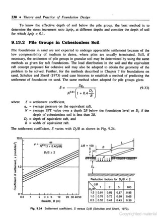
Footings curd Raft Design • 173
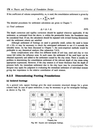
The basic factors which affect the settlement of footings on a give.n soil arc the
intensi<y of loading and 1he size of the loaded area. The senlement increases in almost direct
proportion to these parameters. It is a common experie.nce lhat even though the foundation
pressure is the same under all footings, a bowl shaped defonnation 1rough is obtained with
greater settleme- t at the centre than along the edges of the building mainly due to greater
n
load in the central columns and the overlapping of stresses from adjacent footings. Hence, to
produce uniform settlement. it may be necessary to adjust the pressure with size of footing,
that is. to impose greater pressure under smaller footings than under larger ones and also to
use larger pressure under the footings along the edge of the building. The principle was
u1ilized in the CB I Esplanada Building, Sao Paulo which was founded on moderately
compact fine to medium sand. A pressure of 550 kN/m2 was used under the OUler f()()(ings
and 400 k.N/m2 under the inner footings, with the result that the maximum differential
settlement did no< exceed 8 mm ($kempton, 1955). So, lhe bearing pressure of footings in a
bu.ilding frame may be varied though it is always kept within the safe bearing capacity so as
to have the maxjmum and differential settlement within permissible limits. This may require
a number of Dials before the finaJ design is arrived at. A simple caJculation for achieving
unifonn settlement of adjacent footings is shown in Example 8.4.
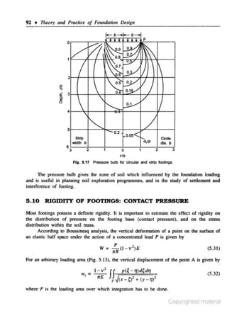
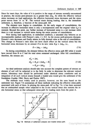
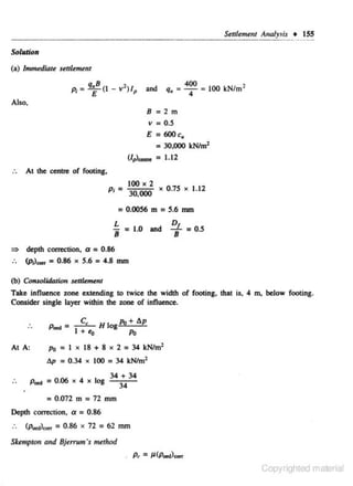
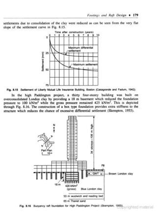
A satisfactory method of reducing the differential settlement of footings in a building
frame is to provide interconnected beams between columns at the foundation level. A framed
slructure is tied laterally, from firs! floor onwards, by beams and slabs but no such
connection is generally provided at the foundaHon level. Consequently. the individual
footings can settle differentially. Providing inten:onnec<ed beams increases the rigidity of the
foundation and differential settlement is subscantially reduc-ed. An approximate way of
analysis would be 10 estimate the settlement of individual footings as isolated/strip footings
and then to design interconnected beams to resist tbe bending moment at the joints due to lhe
differential settlement. For more accurate design. theoretical analysis of the building frame
may be done with predetermined sections of the interconnected beams and footings.
Figure 8.10 shows a 1ypical s:aip foundation with interconnected beams.
~
D D -~;dk,]~
D EJ
0 L! D D
I
I
Section AA
I
_JA
Strip
•
•
I
,.....
I
1/
lnterooonec::te'
I
I
1---
beam
F~. 8.10
•
•
I
I
I
I
I
I
I
I
I
I
~ ~ ~
Strip footings with interconnected beams.
f-
Strip

201. fiHJting.,· ami Raft Design • 179
settlemenlS due 1 consolidotion of the clay were reduced as can be seen from the very flat
0
slope of !he settlement curve in Fig. 8.1S.
0
Tlmt 1n.t OOf'llttuclion
7
•'
I
0
(ye~rs)
a
9 10
,.-
,
Muimum dl'**'lill
t'-...
1.
f'
lr Mo>*num
75
Flg. 8.15
S e - ol ~ -
lkAklilg. Booton (Co_.,.,. -
Life -
FacO.wn. 1942~
In the high Paddington projec~ a thirty four-storey building wu built on
overconsolidated London clay by providins 1 18 m basement which reduced the foundation
pressure to 100 kN/m 2 while the gross pressure remained 425 kN/m2• This is depicted
through Fig. 8.16. The conslNerion of • box type foundation provides extra stiffness to !he
sbUeture which reduces the chance of exce51ive diffe,.,ntial settlement (Skempton. 1955).
N
l
~
.....
8
e
*
~
i
~
Pan Plan
~
0
~
Fll
Brown Lonc:lon clay
m
1• ~
·• •
I~
·20 """"'
(grooal
-
....,_, day
$3 m WIXIIn1ch end ruding bed
6$ m 'ThlnM land
Flg. 1.16 8uoyoncy ...~ -
for High
Poctdiov... PYojocl (Sbmplon.
1956).
edrr"
a

202. 180 • Theory and Practice of Fouudatio11 Dts1
'g11
Glossop ( 1972) indicated two types of floating foundations de- ending on whether
p
floatation is required to reduce the settlement or to prevent shear fai lure of the s ubsoil. In
eithe- case. the net fou ndation pres.ure should be reduced to such an extent that the design
r
criteria with respect 1 both. shear failure of the soil and seu.lemen1. are satisfied.
0
Increased rigidity of fou ndation may be achieved with a buoyancy rofl by providing a
cellular construction below the ground. The s uperstructul'e and the cellular rofl provided for
the Cossipore Power Station, Calcuua is an exceJient example of a near floating foundation
on soft normal Calcutlll deposit. It is shown in Fig. 8.17.
Boiler house
.AIIutar tllf'l
70 m x 100m
6mJ
~lDI
Turt:line house
F=
"
!
100 . f.o~~
"" .
~ o.sm
.
rom
Fig. 8.17 Celular raft founda!lon for Cosslpore " " - Sta!lon, calcutta (Skempton,
1 955~
When the height of a building varies, it is possible to combine rafts under the heavier
part with footings under the lighter pan of the building. A good example of this is fou nd in
the Thomas Edison Building, Sao Paulo, refer Fig. 8.18, where a reinforced concrete mat
with foundation girders connecting all columns was provided under the twenty onc-st· rey
o
section of the building while s pread footi ngs were provided for the ten-storey block. The
maximum settlement at the end of construction was only 15 mm (Rios and P. Silva, 1948).
21
10
Depth (m)
4.9m
~~:j~
--.,::=-=::&---!
5
-~"':-!"'::"----! 10
Fig. 8.18 Combined raft and fooling foundalion for Thomas Edison Building, Sao Paulo
(Rios and P. Silva, 1948).
Copyrighted material

203. Footi11gs a11d Raft Oesig11 + 181
8.3.5 Basement Raft
Buoyancy raft foundation can be conveniently used to provide basements for multistorey
buildings in sofl clay. This gives add.ilional floor space to a building but requires no
additional ground covernge. Depending on the depth of foundation multiple basements mBy
be accommodated. Figure 8.19 depicts Albany telephone building in New York which was
founded on a 7 m deep buoyancy raft with two basement floors. The subsoil consis1ed of
sensitive plastic clay. But the net foundation pressure of 40 kN/m2 restricted the senJement
the building to only 60 mm (Casagrande 1932. Glossop 1972).
or
...
Property
Building line
Chase few
mm
Part< street
cable
vault
Approx. 7 m
1
Mud
lOOm
mat
.
Fig. 1!1.19 t.1urtiple basement for AJ)any telephone building (Giossop, 1972}.
Analysis of buoyancy ran foundation in normal Calcutta soil g.ives some interesting
observations. For a typkal 10 m x 20 m raft. the net foundation pressure is to be rcstricled
to 40 kN/m 2 to keep the senlement within the permissible limit of 125 mm (IS 1904: 1966).
According.ly, the depth of foundation for different gross foundation pressures can be
calculated. Table 8.2 gives the relevant data. II is clear that one, two, or three levels or
basement may be provided within the depth of foundalion to restrict the net foundation
press ure to 40 kN/m2 for eight. twelve, and sixteen-storey buildings respectively. That means,
four upper s toreys can be buill for e::ach basement floor for buildings beyond four s10rcys
high.
Tabl ~
8.2 Depth or b3~ment in normal Calcu n:~ soil
q~
No. of
(tlm'l
s1orqs
4-0
4.0
..
No. of
basem~nl
1
0.0
qiWf • q,_ -
ro,
;;; q.,_ - i .SD1
3.3
4.1
8
1
6.0
6.6
4-1
12
2
22.0
10.0
4.0
16
jiDOrs
3
Copyrighted material

204. 182 • Titeory and Practice of Foundation Df'.sign
Structural Design of Raft Foundation
8 .3 .6
A ro.n foundation can be structurally designed in the same way as the reinforced concrete
floors of a framed building. However. in a foundation raft, the floor is inverted so that its
dead weight can be subtracted from the upward soil reaction.
(a) Rigid method
Raft foundations are mostly designed by the rigid method. This assumes the raft to be fully
rigid and ensure.~ that the deflection of the raft does not affect the soil contact pressure. Also,
the contact pressure is assumed to be distributed on a plane surface and the raf1 is so
proponjoned lhat the line of action of the resultant forces coincides with the centroid of the
contact pressure (Teng. 1972). This assumption appears reasonably valid when sufficient
rigidity is imparted on the raft by the action of the interconnected beams and columns. or
cellular raft or flat slab construction as the case may be. Structural design of the raft is
similar to that of an inverted slab subjected to upward reaction of the ground with support
condition to be obtained for the appropriate design.
To facilitate the design of raft by the conventional rigid method, Hetenyi (1946) has
given an approximate criterion for detennining the validity of the 'rigid' assumption. For
relatively unifonn column load and uniform column spacing. the raft may be considered
rigid if the column spacing is less than 1.75/A.. where .t is defined as the characteristic
coefficient given by
(8.12)
where.
Ks
= coefficient of subgrade reaction {pressure required
to cause unit displacement),
b = width of a strip of raft between centres of adjacent bays,
£(' = modulus of ela.sticity of concrete, and
I = moment of incnia of the strip of width b.
(b) Ewtlc method
In the simplified elastic method, lhe soil is assumed to consist of infinite number of clastic
springs each ac.ting independently. The Winkler model is (."Onsidcrcd valid. The springs are
assumed to be able to resist both tension and compression while the soil defonnation is
considered proportional to the pressure . The elastic constant of the springs is determined by
the coefficient of subgrade re,aclion or the soil (defined as the unit pressure required to
produce unit settlement). The analysis is carried out following the concept of beam on elastic
foundation , the rigorous analysis for which was done by Hetenyi (1946). The raft is
considered a.s a plate and the column loads arc distributed in the surrounding areas in the
zone of influence. The bending moment and shear force are calculated for each column point
and the data are superimposed to obtain the moment and shear for the raft foundation.
American Concrete Institute has recommended a procedure for design (ACI 1966, 1988).
Computer programs are now available to C-il.rty out the comple~ ma h~Yi~~~-~8ulitffit 1
· rnr

205. Footings and Raft Design • 183
practical use. Finite element fonnulation can also be used to work out a computer program.
Given the scope of this book. the details are not discussed here.
Example 8.1
An isolated column in a building frame. with a column grid of 3.5 m X 3.5 m carries a
superimposed load of 450 kN. The subsoil condition is shown in Fig. 8.20. Design a suitable
square footing for the column.
450kN
Depth (m)
0
Fl
1
1 Oesk:leated bt'Owr'!isl'l grey silty day
2
r=
c.,
18 kNim3
= 40 k~; Ccl(1 + So)
4
=0.05
II Grey silty day
r = 18 kNfm'
c., = 25 kNffnZ
C,/(1 • sol = 0.16
12--------------------------------- kankar
Ill 8tul$h
silty
with
grey
day
r• 19 kNtm'
c., = 60 kNfml; CcJ(1 • So} = 0 .10
16
Fig. 8.20 Subsoil condition for Example 8.1.
Given superimposed load = 450 kN
Take footing size
=2 m x 2 m
450
2
q..,=2 x2 = 112.5 kN/m
Place foundation below fill and at depth of G.W.T. i.e.
v,= 2m
Solution
(a) Bearing capociry
N,
= 5(t + 0.2
~)(1 + 0.2 ~)
= 7.2
Failure surface lies in Slnllum I. Hence, take c, = 40 kN/m2.
Copyrighted material

206. 184 • Theory alld Practice of Foundan'orr De.sigtr
Cohesive soil:
Qu11(n)
= c.,N~
: 40
X
7.2
•
= 288 kN/m•
~.
r. -
288
112.5 = 2 '56 > 2 ' 5
(b) Immediate settlement
q. = 11 2.5 kN/m2
B=2m
v = 0.5
IP<~"'>
E
= 1.12
=600c. =600 X
32
= 19,200 kN/m2
Stress innuence zone extends to equal depth in layers I and
n. Therefore. weighted
average
is
.
..
c• =
40
X
X
2
4
and
p,
2 + 25
= 32 kNim'
= q£B o - v')l,
=
112.5 X 2
19,200
X
0.75
X
1.12
= 0.0098 m
Depth correc.tion (Fig. 7.3)
D
.fi.i
L
B
and
=
2
N
=1
=1
Correction factor = 0.73
(p;)"'" = 0.73 X 0.0098 = 0.007 m = 7 mm
(c) Cb, solidation settlemellf
Pr = "" C, H lo P. + llp
L... I + "o
g
Po
Influence zone extends to depth of 4 m below footing, that is, 2 m in stratum I and 2 m in
stratum II. Hence, consider settJement due to both.
Copyrighted material

207. Foorings a11d Raft D.sig11 • 185
=
=
AI A : Po 18 x 2.0 + 8 x 1.0 44 kNfm1
6p (for ZJB = In) = 0.6 x 112.5 = 67.5 kNt m'
At
8 : p 0 = 18 x 2.0 + 8 x 2.0 + 8 x l.O = 60 kNtm'
,
6p (for ZIB = 312) = 0.15 x 112.5 = 16.9 kNfm·
2 I
p,. - 005 xxog ( 44 + 67.5 ) +0. 16 x2 1og ( 60 + 16.9)
.
44
60
= (0.041 + 0.034) m
= 0.075 m
Depth correction = 0.73
Pore~pressure
correction, J1 = 0.7
(Contribution of layers I and 11 are nearly equal. Hence, take p. = 0.7)
..
(p,),,.. = 0.73 x 0.7 x 0.075
=0.038 m = 38 mm
ToU1 seulemenl, p1 = 7 + 38 = 45 mm
The foundation is therefore adequa1e
Example 8.2
Design a slrip foundation for !he column row C in the building frame shown in F1g. 8.21.
The soil data are also given in the figure.
Oeplh (m)
0
1
";i~~~~
I Brownish grey silty
-l~~ ,' lc 2.5 m .-l'~---r-;_19kNi,;,---- clay
E
j
N
'
+A
~
0
0
I
___
_ ..._
2
0.06
I
E
35 kNfm
Cc/(1 + Oo) •
I
3
tv =
+ B
,'
,
' ,,
I
...... __ ...,.,/
.;:
II Grey organic day
r = 18kNim!
Cv = 20 kNfm2
C,/(1 + ~Jo) = 0.15
0
-~ '~·--~~~~--~
·1
4@ 3.5 m
12--------------~--------------(b)
(OJ
Fig. 8.21
Building frame (Example 8.2).
Copyrighted material

208. 186
t
Theory and Practice of Fotmdation De.sig11
Total load, Q," = 550 + 600 + 600 + 500 + 500 = 2750 kN
Take footing of size = 17 m x 2.5 m
(that is, extend length of footing by 1.5 m beyond outermost columns)
. . q," =
27 50
= 65 kN/m2
17 X 2.5
SoluJion
(a) Bearing capacity
N, =
s(l
+ 0.2
t )(1
=
s(1
+ 0.2
1)(1
+ 0.2
25
+ 0.2
n
~;)
= 5.6
: 35
X
5.6
= 196 kN/m2
Failure zone is resuicted in stratum I. Hence, take c.. of stratum I.
Fs
= 196
65
= 3.0 > 2.5
(b) Immediate sttlltnrtnt
q 11 = 65 kN/m2
8
= 2.5 m
v = 0.5
lp =(for UB = 17125 = 6.8) 2 .32
E = 600 c. = 600 x 26 = 15,600 kN/ m2
Influence zone extends to 2 m in suatum I nnd 3 m in stratum II. Therefore. wejghted
;:~vcroge.
2
X
35 + 3 X 20
= 26 kN/m2
5
And
q.B (l - v}'t
E
=
65 X 2.5
,
15 600
P
X
0.75
X
2.32
= 0.0 18 m
Copyrighted material

209. Footi11gs and Ruft Desigu •
187
Depth correction:
- =L
8
17
= 6.8
2.5
D
=
JL8
1.5
,)2,5
X
J.7
= 0.23
Correction fac tor = 0.95
(p;},0 rr
= 0.95 x 0,018 = 0.017 m = 17 mm
(c) Collsolidation seltlemetll
""
C,
L...1
+ t>.o
H log p., + flp
Po
Two layers (I and If) are involved in the pressure influence zone.
At
A: Po = 19 x 1.0 + 9 x 1.0 = 28 kN/m•
'
flp [for Z/8 = 1.6/2.5
At
B: Po
= 19 x
1.0 + 9 x 2.0 + 8 x 1.5
flp (for Z18
...
~
= 0.4] = 0.85 x 65 = 55.2 kN/m·
'
= 004
.
=49 kN/m2
= 3.512.5 = 1.4) = 0.42 x 65 = 27.3 kN/m 2
x
21
og
28 + SS.2
D
0 IS
+ .
x
21
•
49 + 27.3
49
= O.Q38 + 0.058 m
= 0.096 m
Depth correction
= 0. 95
Rigidity correction = 0.8 (lnrerconnected strip provides rigidity to the foundation)
Pore-pressure correction. J1 = 0.75
(Major contribution to settlement comes from strata I and II. Hence. J1 correction for N.C.
clay is considered.)
..
(p,)""' = 0.95 x 0.8 x 0.75 x 0.096 = 0.055 m = 55 mm
..
Total setdement. p1
= 17 + SS = 72
mm < 75 mm
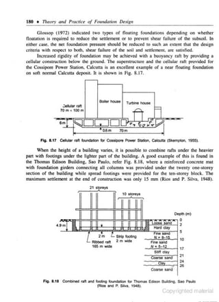
Example 8.3
A column carrying a superimposed load of 1500 kN is to be founded in a medium sand as
shown in Fig. 8.22. Design a suitable isolated footing.
Copyrighted material

210. 188 • Theory and Practice of Foundation Design
1SOO kN
N {Biow>/30 em)
Depth (m)
o--------~ ~~~----~~~~r;
18kNim3
2 --¥,.-,,..-----,
,. . ."'
.
I
-
i
-5m
Fig. 8.22 Example 8.3.
Nu., = 15
Average N value,
f =
34° (Eq. (2.5))
N, = 30
N1 = 41
Q... = 1500 lcN/m2
Assume footing size = 2.5 m • 2.5 m
.
qftll!f.=
"
1500
_ • _ = 240 kN/m'
2 5 25
Solution
(a) Bearing capaciry
•• = 1.2; s, =0.8; dq =d, = 1.15; ;, = ;, = 1.0
q,.(n) = q(N, - l)sqd,i, + 0 .5yBN1s1 d1 i1
= (J8
K
2(30- I)
K
1.2
K
1.15
K
1.0) + (0.5
X
9
X
2.5
X
41
X
0,8
X
1.15
X
1.0)
= 1440 + 424
2
= 1864 kN/m
Fs =
1864
= 7.8 > 2.5
240
(b) Settlement
Considering single layer of 5 m depth
S
=
2
·~·
fl log Pn + l!.p
Po
Copyrighted material

211. Footings ami Rafi Design • 189
p. = 18
l!.p
E
X
2 + 9
X
2.5 = 58.5 kN/m2
= (for 718 = 1.0) = 0.35 x 240 = 84 kN/m2
= 39 + 4.5 x IS = 1065 kg/cm 2 = 10,650 kN/m2 (refer Eq. (2.6))
6 =
2.3 X 58.5
I 58.5 + 84
x 5 og
58.5
10,650
=0 .024 m
= 24 mm
EXample 8.4
Three columns in a building frame spaced 4 m apart carry vertical superimposed loads of
500 kN, 720 kN and 600 kN. Design suitable isolated footings for the columns for equal
settlement. Subsoil condition is shown in Fig. 8.23.
Depth (m)
o --------~RI
~-------,-.~t77
s k~Nhn~,------
-• - ~----------------------I Medium day
r• 18 kNim,
c;. = 40 kNhn'
m~ = 0.0005 m'lkN
-s----------~-----------11 SUff Clay
r=
19 kNim1
c;.. 90 """"'
0.0003 m21kN
-1
0----------=....::;=:.:.::..=-----m.. •
Fig. 8.23 Subsoil condition (&ample 8. .4).
Solution
Approximate q.,,(n) of slr.ltum I
= cll/Nt:
= 40 X 6.0 = 240 kN/m2
qo~,(n)
.
= 240
25
,
= 96 kN/m- (for Fs = 2.5)
Choosing approximate fOOting size accordingly and carrying out detailed analysis.
Column A
Take footing size = 2.2 m x 2.2 m
Area
= 4.84
m2
500
2
q..,. = = 103.3 kN/m
4. 84
Copyrighted material

212. 190 • Titeory and Practice of Foundation Design
(n) Bearing copaciry
Failure surface in layer 1: Take c. = 40 I<N/ m2
N,
s(I 0.2 ~ )(I 02 ~)
.
=
+
+
: 5( 1 + 0.2
X
1
) (1 + 0.2
22
X
1)
= 6.55
Qu
n(n) = cMN('
: 40
6.55
X
= 262 I<N/m2
262
. = 2.54 > 2.5
103 3
Fs =
(b) Immediate senlemelll
q. = 103.3 I<N/m2
8
= 2.2
m
v = 0.5
lp = 1.12
E = 700 x 40 = 28,000 kN/m2
P; = q. B (I - v 2) / P
E
: 103.3 X 2.2
28,000
= 0.007 m
X
0. 75
X
1.1 2
Depth correction:
D
I
JL.B = 2 =0.5
L
8
= 1.0
Correction factor = 0.85
(p1),.,
=0.007 x 0.85 =0.006 m = 6 mm
(b) Consolidatio11 selllemeJI/
p, = Drr,t,pH
At A:
l'lp (for
= 18 x 1.0 + 8 x 2.2 =35.6 kN/m2
lJB = I ) = 0.35 x 103.3 =36 kNim'
Po
Copyrighted material ·

213. Footings and Raft Duign + 191
..
Pt- = m.,tjpH
: 0.05
X
36.5
X
4.4 = 0.080
ffi
Deplh correction = 0.85
Pore-pressure coJTeCiion = 0.7
(p,)...,. = 0.85 x 0.7 x 0.08 = 0.048 m = 48 mm
p1 = 6 + 48 = 54 mm
Column B
Take footi ng size of 3 m x 3 m
Area =9m 2
q,.. =
720
= 80 kN/m2
9
(a) Bearing capaciry
N,
I
= 5( + 0 .2
= 5(1
~ ) (I + 0.2
+0 .2
X
n
1
2
9)<I+ 0.2)
= 6.4
qulc(n) = C11N~
: 40
X
6.4
= 256 kNtm'
Fs
= ~ =32
80
.
(b) lmmed,.ate settlement
q.
= 89
kNtm'
8 =28m
v = 0.5
Ip(..,ey
= 1.12
40 x 4 + 2 x 80
6
= 53 kN/m2
Influence. zone ext· nds approximately to 4 m in stralum I and 2 m in stratum II. Therefore.
e
weighted average taken is
Copyrighted material

214. Practic~
192 • Theory and
of Foundation
£
=700 x
Pr =
=
q•/
D~sign
=37,000 kN/m2
53
(I - vl)IP
80 X J
37,000
-
X
0 .75
X
1.12
= 0.0054
. Depth coJTection:
L = I
B
D
JLB
= 0.33
..
Correction factor = 0.9
..
(p1)..,. = 0.9 x 0 .0054 = 0.005 m = S mm
Consolidation
settJ~ment
Pc = Lm~~6.pH
= (0.0005
X
4
X
36.8) + (0.0003 X 2 X 9.6)
for point A(ZlB = 0.66), 6p = 0.46 x 80 = 36.8 kN/m2
= 0.074 + 0.006
for point B(Z/B = 1.67), 6p = 0.12 x 80 = 96 kN/m2
= 0.080 m
Depth correction
= 0.9
Pore-pressure correc1ion
= 0.7
(p;)""' = 0.9 x 0.7 x 0 .086 = 0.050 m = SO mm
p1 = S + SO = SS mm
Column C
Take footing size or 2.5 m
X
2.5 m, and
area = 6.25 m2
q.,
600
= 6_ = 96 kN/m2
25
Sellltm~nt
By similar calculation as in the previous pans,
p, = 5 mm
p, =SOmm
P =5 +50 =55 mm
t
Copyrighted material

215. Hidden page

216. Hidden page

217. Hidden page

218. Hidden page

219. Hidden page

220. Hidden page

221. File Foundations
9.1
IN'fRODUCTION
Piles arc relatively long and slender structural members used to transmit foundation loads
throu~ soil of low bearing capacity to deeper strata (soil or rock) having high bearing
capacity. They are also used in normal ground conditions to resist uplift and lateral forces.
The principal uses of piles are:
I. To carry vertical compression load from builclings, bridges, and so on.
2 . To resist horizontal or inclined loads by retaining wall, bridge pier, water front
structures and structures subjected to wind or seismic loads.
( 3. To resist uplift forces in transmission towers and underground structures below water
table.
·'
Piles are described as end bearing piles and friction piles depending on the manner in which
· the load is transmitted into the surrounding soil. These can be defined as follows:
~
If the pile rests in a hard and relatively incompressible suatum, for example, rock or
dense sand/gravel, the pile derives most of its carrying capacity from end bearing at the pile
tip. Such piles are called end bearing or pcint-bearing piles. Figure 9. 1(a) depicts endbearing piles. The soft compressible layer through whic·h the pile passes may not carry any
significant load by side friction.
0
0
t t
Soft orouod
Soil propeftieS
imp!O'Ing with depth
but no ftnn ground
Is reached
Frm ground
{a) End bearing pie
{b) FrictiOn pile
Ffo. 1.1 Pile:s: methods of lOad transfet'.
199
Copyrighted material

222. lOO • Theory and Practice of Foundation De$ign
If the pile does not reach an incompressible sttatum but is driven for some depth into a
penetrable soH, the carrying capacity of the pUc is derived primarily from skin friclion or
adhesion between the embedded surface of the pile and the surrounding soil. Such piles arc
called friction piles. as shown in Fig. 9.1(b).
Although. in common terminology, piles are often referred to as friction piles or end·
bearing piles-in reality. there is no pile that ttansmits the load to the surrounding soil solely
by fricr ion or solely by end bearing. The distinction only serves to indicate the relative
magnitude of the load that is transmitted by friction and by end bearing. For example, a
S!raight pile embedded in homogeneous c lay will mostly ttansfer the load by friction and a
pile wid& its tip resting in dense sand underlying soft clay can be considered an end bearing
pile.
The relative magnitude of the, skin friction and the base resistance of a pil~, however.
:.
depends on various fac tors such as~
1. Geometry of the pile shaft-its shape, length, and diameter and whether it is with or
without enlarged base.
2. Subsoil slratification along the pile shaft and the properties of soil in which()be pile
is embedded and where the tip of-the pile rests.
3. Method of consl!Uction of the pile. that is. driven pile. bored pile, and so on.
9 .2
CLASSIFICATION
Piles are classified according to their composition or method of installation.
I
9 .2 . 1 Claaaificatlon Baaed on Compos ition
I
(a) TimiHr pihs: In India, timber piles arc mostly made up of sal l!Ce l!Unks and arc'
called salballah piles. These arc commonly available in length between 4-6 m. with
diameter nonging from 15-25 em. These may be suitable where good bearing sl!atum
is available at a relatively shallow depth. Now a days. use of timber piles is
restricted due to the necessity for preservation of forests.
(b) ConcrtU piles: Concrete piles are either precast or cast·in·situ. Pr~casr piles may
be of various shapes but are normally suitable for short lengths. These piles should
be adequately reinforced to have sufficient structural strength to withstand handling
stresses. With precast pi les~ it is possible to have good control on quality as they arc
cast on the ground before installation.
Cast·in-situ concrete piles are commonly used where relatively long and large
diameter piles with or without enlarged bases are required to support heavy loads.
(c) Stu/ pihs: These arc usually of tolled H sections or pipe sections. These piles may
be used where less disturbance from driving is desired. H-piles and steel sheet piles
are commonly used to support venical sides of open exc- vation. Steel sheet piles are
a
also used to provide seepage barrier.
Copyrighted material

223. PUe Foundations • 201
9.2.2
Classiflcation Based on Method of Installation
(a) Drit~tn pil~s: These may comprise of timber, steel. or preca.~t concrete. The piles
are driven by the impact of a hammer or by vibrations induced by a vibratory
hammer.
When n pile is driven inro the soil, i1 displaces a volume of the soil equal to the
volume of the pile. So. these piles are also called disp/acemem piles. In granular
soils. the driving operation densities the soil and increases strength of the soil in the
vicinity. When piles are driven in saturated clay, the soil instead of being compacted
gets remoulded often with reduction of strength. The soil, however, regains strength
with time due 10 consolidation and thixotropic hardening. Because of the
displacement of soil by !he piles, !here may be ground heaving around the piles.
/"~Jso, driving of piles impartS vibratjon to surrounding soil. which in some cases.
' may be detrimental to struciUres located very close to the site.
(b) Driven c4st-in-silu-pilts: These piles are also a kind of driven pile. Steel casing is
J driven into !he ground wi!h a shoe a! the bonom. The hole is then filled up with
concrete, and the casing is gradually lifted as the concrete is poured.
(c) Bo,..d piltf: These piles are formed in prebored holes in !he ground either using a
casing or by circulation of a drilling Ouid, such as bentonite slurry. Concrete is
poured into the hole by displacing benloni!C and then gradually lifting !he casing.
'
f
•
'i
~
Bored piles may be of the following types:
(i) Small diametes bored piles-generally up!o 600 mm diameter.
(ii) Large diameter bored piles- diameter generally greater than 600 mm. They are
advantageous where heavy structurnl loads are to be supported.
(iii) Under.reamed piles-one or more bulbs of larger diamerer than that of the shaft
are fonned by s-uitably enlarging the borehole with special tools ro increase the end
resistance. These piles are suitable when a good be.aring s1.ratum is available at a
relatively shallow dep!h. The uplif! capaci!y of these piles is high. In India, these
piles are widely used to provide suitable foundations in expansive soils.
Bored piles are noll·displacement piles and may be used when pile driving is
detrimental to adjoining structures.
9 .3
PILE BEHAVIOUR UNDER AXIAL WAD
figure 9.2 shows a typical load seulemen! diagram for a pile under gradually increasing load.
At small dcform~tjons. say upt'O the point A in the figure. the piJe,..soil system behaves
elastically. as indicated by !he linear load ' 'ersus scttlemcm relationship. Up1o !his poin!. !he
entire load is carried by skin frictio n and there is virtually no transfer of load to the pile tip.
Vith more deformation. the pile shaft carries more frictional fon,-es while a part of the load
is transferred to the pile tip also. At 8 , the pile tip carries the ma.ximum skin friction that
can be mobilized in the soil. Therefore. funhcr increase of load on the pile is carried out at
the pile tip and the pile is said to have failed, at C. when the tip lood has also re:~ched its
Copyrighted material

224. II
!!
"
202 • TJreory and Pracn'ce of Fomula1itm Design
maximum value. Thus. the load c.arrying cap ily of a pile may be determined from separate
evaluation of the ultimale skin friction and t ultimate base resistance.
o1
I
I
Tolal
c
t
Oispl~nt --+
Fig. 9.2 Load settl
t relalionshlp ol plies.
Thus.
where
•
'
wp- w,
Q• is the load carrying capacity of
a, is the maximum skin friction on
pile.
e pile shaft,
Q. is the ultimate tip resistance,
WP is the weight of the pile. and
W, is the weight of soil displaced b 'the pile.
•
In general. w. and W, are small in relation to QP and their differences even smaller. Thus.l
for practical purposes
Q, = Q Q.
,
(9.2) ~Therefore. it is apparent, that full mobili 'on of Q1 and QP are primruily dependent on •
the movement of the pile in the soil (refer Fi . 9.2). Cooke (1974), and Cooke and Price
(1973) have shown that. for an clastic soil, ful mobilization of skin friction in a cylindrical
pile occurs at vertical displacement of O.S-1% of the pile diameter. On the other hand, full
mobilization of base resistance requires a muc greater ddormation-even upto 20% of the
base diameter (Whitaker. 1976). This suggcs that skin friction is mobilized almost fully
before any appreciable base resistan<-e develo in the soil. Therefore, the entire problem of
load distribution through piles has to be 'iew as a pi~e-soil interaction where the response
of the soil to a given deformation in terms of 'n friction and end bearing has to be taken
into account.
An evaluation of the zone of soil that is i nuenccd by piling is important to detcnnine
the soil propenics that come into play in resi ting the movement of the pile in the soil.
Meyerhof (1959) and Kerise1 (1961) consider+ the influence zone as shown in Fig. 9.3.
According to Meyerhof (1959), the shear zone~ the base causing beruing capacity failure of
the soil e"tends to !Qme distance above the
tip. The zone of skjn friction may extend
laterally to a distance of three to fou r times the iameter of the pile while compaction of lhe
pile m11y occur upto a distance of five to six mes the diameter. Cooke and Price (1973)
have. however, observed that displacement of
soil may extend to a radial distance of ten
pili
thl
Copyrighted material

225. Pile Fount/Qtions
+ 203
diameters around the pile. Pile driving cause.~ significant changes in dte soil within the zone
of influence. Therefore, it is important to study the various fac.tors that affect the soil during
piling.
p
•
Ag. 1.3 Stress Influence zone around piles.
9 .4 ~ PILE CAPACITY TO RESIST AXIAL FORCES
The load carrying capacity of a pile is controlled by its suuctural strength and the supporting
strength of the soil. The smaller of the two is considered for design purposes. These are three
apporaches to the computation of pile capacity based on soil support. These are:
..•
(a) Static analysis
(b) Dynamic analysis
(c) Load test
t 9 .4 .1 Structural Capacity of Pile.
The structural capacity of a pile is its strength as a column. When the pile is completely
embedded in soil, the restraint offered by the soil is generally sufficient to consider the pile
as a short column (except for the case of a long pile in very soft clay). Pre-cast concrete
piles are adequately reinforced to withstand handling and driving stresses. Cast-in-situ piles
are also reinforced to increase column strength and also to resist moment that may have
developed due to horizontal load or eccentricity of vertical loads. Reinforcements are also
fielpful in resisting tensile stresses that may develop due to heave resulting from driving of
adjacent piles in clay.
9 .4 .2
Pile Capacity from Static ADalysia
The static analysis relates the shear strength of the soil to the skin friction along the pile
shaft and end bearing at the pile tip. The carrying capacity of a pile is given by the sum of
the ultimate bearing capacity of the soil at lhe pile tip and the ultimate adhesion between the
pile and the surrounding soil, (refer Fig. 9.2).
(9.3)
Copyrighted material

226. 204 • Theory and Pracrice of Fowufatiott Design
where
/, = unit skin friction in each layer.
AJ = pile area providing skin friction in each layer.
A, =pile area providing end bearing, and
q, = ultimate bearing capacity of soil at pile lip.
Pile. in cohesive soU
A total stress approach is generally used to determine the shaft and tip resistances of piles in
tohesive soil considering that the load transfer from the pile to the soil occurs under
undrained condition.
Driven pil~s: When n pile is driven into a cohesive soil, two effects of pile driving become
significant.
J
The clay is displaced laterally and in an upward direction, resulting in a ground heave.
The soil close to the pile shafl gets disiUrbed to cause remoulding of the clay. This may lead
to considerable loss in strength of the soil. This has been discussed by Flame (1972! who
observed appreciable increase in wat· r content and corresponding reduction of shear strength
e
of the soil between two adjacent driven piles in clay. With time. soft clay regains this
strength either completely or partially by thixotropic haroening (Skempton and Northey,
1952). A corresponding increase in load carrying capacity of the pile with time is shown in
Fig. 9.4 (Tomlinson. 1994). On the other hand. in stiff c lays, extensive crocking or the soil
occurs during pile driving. Clay in the upper part of the pile breaks away from the shaft and
nury 11ever regaitr contact with it (fomlinson, l977). Thus, the effect of pile driving on thilt
shear strength of the clay differs with the soil consistency. Considerable gain in strength may •
be observed with time in sofl clays while no appreciable effect may be noted in stiff clays.
loor---~~-r~~-rfTTr----ll--~r-Tllfrn-=::=t~J=~-~ ffl1l1
r.-· .- 2
'5ll-:;200;;;;-:-,-'.;2~15;-:m:m:-'cooae:::::::t::.-ttt-----t--tp-t-.:;le.f:fTt.r.~~"·~=-·---~-..-. .-. t-. t... .rt:-.11H 25 o;
·
. ~.-.. - t.-t . .
~
=
(Gothooburg)
..... .- · - - .
... ·· ·
E
-200
-r-::::"'::;;-~~~"'+""f+l+t-tt---t-HH+t+tl20·
lt50
.- -· ... . . ~-· ....
15
30
'ln......
0
.. ·.... ··· ~.,..
·-
t- ~50 x
f
v
150 mm tal)e(ed
.Wt00'f-:~~;_·~1-··..,.¥/?l-<4-++++l-..:1imbe:::=:::'..:1::0...m;:m:::en~)'-..--~-----i--l--HH+i+l to ~
· '
::::;
!
:·If·
50
l0 /
150 mm (8 in) steel
/ ~ 125 mm t-Beam+---~,:"'::be:::.;I:::S•:.;•;...:,Fra;.::;: ·•:;co:;)T-----I--+-+-++++H 5
na:;
o /~ lG~~i:1'2h
1
5
r rr --,_
10
50
tOO
500
:
a>
tOGO
Time after driving (days)
Fig.. i.4
Gain in load carrying capacity with time of driven piles in soft clay (Tomlinson. 1994).
High porc·prcssure is developed in the c lay due to pile driving fo rces. This porepressure often takes time to dissipate. When reconsolidation of the clay occurs, the soft clay
Copyrighted material

227. Hidden page

228. 206 • Theory and Pracll'ce
<if Fomulntiou Design
9.5 FRICTIONAL RESISTANCE
Ve have. so far discussed the various factors that affect the soil during pile driving. The
quantitative evaluation of frictional resistance should take into account the effect of all these
facwrs on the shear be-haviour of the soil. Although the frictional resistance is basically a
function of the shear sltength of the soil, this friction develops as an adhesion between the
pile and the soil ;md not as pure friction between soil particles. The c·omplex nature of
stresses developed around a pile. the effects or remoulding and/or stress release of the soil.
and a some what indete- minate nature of the pore-pressure dissjpation and pile soil interaction
r
make it difficu1t to have a precise evaluation of skin friction.
Paton ( 1895) applied Rankine's earth pressure theory to obtain the bearing capacity of
piles (see Whitaker, 1976). The frictional resistance along the pile shaft was expressed as,
F,
1.1 - s inp
I
. ,. A,
= Pr -2
,
•
+ sm.,..
(9.4)
J1 is the coefficient of friction between the pile and the soil,
is the density of the soil.
l. is the length or the pile.
'
(J is angle of internal friction of the soil, and
A, is surface area of the pile.
Tl1e major uncertainry in using Eq. (9.4) to evaluate the skin fTiction lies in the
estimation or p and (!of the soil. In particular. no di<tinction is made between clay and sand,
and the choice of these parameters for actual conditions that exist around a pile during and
afte- driving leads to difficulties.
r
~
Burland (1973) developed a method of calculation of shaft friction from the e ffective
stress principle. It is assumed that the zone of distortion around the pile being small, the
porc·pressure dissipates quickly and Joading takes place under drained condition. It is further •
assumed that there is no effec.::tive cohesion in the soil due to remoulding of the soli around
the pile. The unit s kin friction at any depth is then given by.
where
r
•·
[, = kp tan 8
where
(9.5)
k is the lateral earth pressure coefficient.
p is the effective overburden pressure at the depth considered. and
8 is
the angle of friction between the pile and the soil.
It poses extreme difficulties to seJec,t appropriate values of k and p. p is initially s mall due to
high pore·pressure developed during driving but its value soon increases with dissipation of
pore water pressure. In driven piles. k is also likely to be high initially because or the driving
forces whereas in bored piles, k will be small due to swelling of the soil. These values may
ulti mately attain some s tability after installation but uncertainties stiiJ remain regarding the
time required for drainage of the soil around the pile and about values of k and p that should
be applicable in a field situation. Burland made a further simplifying assumption that k = ko
(k0 is the coefficient or earth pressure at rest) and obtained the following expression for the
total shaft friction:
L
F, = JTB
L pko tan 8(A£.)
0
(9.6)
Copyrighted material

229. Pile Foundations • 207
Owing to the uncenainues involved in selecting fie ld parameters for analytical
solutions. attempts for evaluation of friclional re..~is1ance of piles have been based on semi ~
empirical approaches.
9 .5.1 Frictional Resistance in Cohesive SoU
When a pile is installed in a cohesive soil, e ither by methods of driving or boring. the
immediate defonnation of the soil takes place essentially under undrained condition. In this
case. ; : 0 analysis (Skempton, 1948) would be valid. The unit skin friction between the soil
and the pile may lhen be considered 10 be a function of the undrained shear srreng1h of the
clay. Notwithsmnding the fact that this shear strength may undergo change with time due 10
thixotrop hardening or due to dissipation of excess porc·prcssure. the unit ultimate skin
jc
fricdon) nay be expressed by the equation,
[, = ac,
(9.7)
c, is rhe undrained shear strength of the clay. and
' a is an adhesion factor.
where'
The total fricdonal resistance of the piles would then be.
(9.8)
where At is the surface area of the pile shaft in contact with the soil in different layers .
.;; While the undrained s hear strength of the clay. c,. can be determined from field vane
· shear test or from laboratory triaxial test. a proper assessment of the adhesion factor is
required for the evaluation of tbe unit skin friction. This adhesion factor gives a measure of
, the part of the undrained shear strength of the soil that is mobilized as skin fric tion.
~
Driven pUeo In cohesive soU
Extensive research by Tomlinson (1965, 1977) has shown that the adhesion factor depends on
the consistency of the soil, as represented by its cohesive strength. In addition. the
penetration depth of the pile appears to have some effect on the adhesion fac tor.
Figure 9.5 illus trates following three different cases.
(i) In the case of short piles in uniform clay, the gap formed near the pile during
driving may occupy a large part of the penetration depth. The average adhesion
factor would. accordingly, be low. For large penetration depth, the gap would be
small compared to the pile length and a higher average adhesion factor may be
adopted. Figure 9.S(c) shows the variation of adhesion factor with undrained shear
strength for piles in uniform clay.
(ii) If the pile is driven through a soft c lay with an underlying stiff clay, a skin of soft
c lay would b!: dragged into the gap formed near the lop of the stiff clay. This would
reduce the adhe.~ion over a cenain length of penetration depth into the stiff clay, the
effect being more predominant in the case of short penetration lengths. The
corresponding adhesion fac tors for different values of c" are shown in Fig. 9.S(b).
Copyrighted material

230. Hidden page

231. Hidden page

232. Hidden page

233. PU~
FoutulaJions • 211
The unit skin friction, according to Eq. (9.1 0) varies linearly with depth along the pile
shaft. This is shown in Fig. 9.8. The total frictional reaistance for a pile of depth D1 can be
obtained as
(9.11)
~
K..-,
Dt
«t~t~l
_},
_.,
1<7' O,tan I
flo. • •• ~ -
In ploo -
Nnd.
where,
A1 is the amo of the pile shall In contaet with the soil and
y' D is the effective overburden JniSUre at the pile tip.
1
The values of K, and 6 as given by Broms (1966) are shown in Table 9. 1. While K, is
a furu:tion of the relative density of the soil. 6 is related to the angle of shearing resistance of
the soil and the nature of pile soil contact. In plies with liner. the sldn friction is even less
than direct soil-concrete friction and a reduced value of 6 should be used.
Tobie u
Values or K, ond 6 (Broms 1966)
ltuiiJIIatiort IN!f/tod
Driven piJes, luse displ~eement
Driven piles, small displace.ment
Bored and ca:st-in-s.itu piles
P//t'-«)U lrttttfact
I.S-2.0
S1t<Vsand
O.S~'-<1.7f
1.0-1.5
.......... <oncmclsand
0.7- 1.0
Cut-in-siN cona'ttdsand
0.8f-I.Of
I.Of
DriYen pllet1 lD cobeeloDieH ooU
In driven piles, Poulos and Davis (1980) have recommended the
6.! ~·
+ 100
UK
of the relationship
(9.12)
to dewmine the angle of pile soH friction ICCOUnting for the effect of pile driving, f being
the angle of shearing real StanCe prior to installation of the pile. However, a value of 6 greater
than ~· •hould no< be used in view of the wide variation of driving methods in the field.
Tomlinoon (1977) hu indlea!ed a relationship between aventge unit skin friction and
relative density, bued on the reauh• of actual pile !Old tesa. as depicted by Fig. 9.9.
According 10 litis relationohip, the skin friction auains 1 petk value of 107 kN!m' (10 !lmlj
foe high relotive density.

234. Hidden page

235. Hidden page

236. 214
t
Theory and Pracr;ce of Foundar;on
D~sign
10,000 .----.---.-----,-----r--,--,
02~5------~
30~----~35~------.~~----~.~5------!
0
Angle ol shearing resls1anoe, f'
Fig. 1.11 Vl111tlon ol N, 1'(111 f' .. obCaiMd
by dl~erent ln-tlga-.
It can be seen that Terzaghi (1943) gives the lower bound and De Beer (1970) gives
the upper bo<Jnd values of N,. Comparison of observed point resistances of piles in sand by
Nordlund (1969) and Vesic (1967) reveal that N 9 values established by Berezantzev et al.
( 1961) give better estimates of point resistance. Although N, values of Berezantzev are
dependent on the relative embedment depth DtfB, the variation is small. An average
Berezantzev curve has been given in IS 2911 (pan I, 1979), Fig. 9.12.
Copyrighted material

237. Pilt Foundations • liS
~-H~tHH+tH+tHK+t~trH+tH~Hi+rttH
~-rHH~++~~++.~Hit+~~t+~Hi+t~HH
•o-+rrt+t+~HHbHRH~14+t++++++t+HHHHHH~HH
~-rHH~++~~++~Hit+HH~t++HHi+t~HH
10 -L~~~LLLUUUUUUU~~~~~~LUUUWU~WW
:zs.o
27.5
~.o
32.s
35.o
lw;Je or.~
37.5
-o.o
•2.5
- ..... (~1. .)
f lo. 1.12 Var1alion d N• -
.-
'5,o
t-nttov, 10&1 ~
z,
j_
9. 7
CRITICAL DEPTH
The effective overburde, pressure required for c.alculadon
n
or friccionol
resistance and end
Co, ynghted matenal

238. Hidden page

239. Pi/~
9 .8
Foundation., • 217
PILE CAPACITY FROM IN-SITU SOn. TESTS
The methods of dete- mination of axiaJ Joad copac ity of driven and bored piles as described
r
earlier in the Chapter, make usc of the shear strength parameters of the soil as detennined
from laboratory testS. For cohesive soils. the undrained shear strength. c" can be detennined
from the field vane shear test also. For sensitive clays, in particular. sampling disturbances
may cause reduction of the cohesive strength of the soil. Vane test results may be
conveniently used in such cloys.
For cohesionless soil. the angle of shearing resistance of the soil is best determined
from the standard penetration te.~t. This test is performed at different depths within boreholes
and the average N value for a layer is related to the angle of shearing resistance. f .
A number of semi-empirical relationships have been proposed to obtain the skin friction
and end resistance direcdy from the standard penetration test and static cone penetration test.
Thorburn and MacVicar ( 1970), based on their experiences in Scotland, proposed an
empirical form ula for the evaluation of pile capaciry direcdy from the standard penetration
resiSUUICe of the sand as
Q. =
;:;
6" A1 + 4NA,
(9.19)
!annes
where A1 is area of pile strength (m2).
A, is area of pile tip (m2),
N is the average N value over the pile shaft. and
N is the SPT value at pile ba.o;e.
Tomlinson gave the relationship for ultimate bearing capacity of displa.:ement piles
from static cone penetration test.
(9.20)
where
qr- = cone resistance in Vm2 at pile tip. It is taken as the average value of cone
resistance over a depth equal to three times the pile diameter above the tip and
one pile diameter below lhe tip,
A, = area of pile tip in sq. m.,
i r = average cone resiS"tance over the embedded length of the pile shaft. and
A1 = surface area of pile shaft in sq. m.
For taking unit base resistance as qr• the pile should penetrate at least 8 diameter into the
bearing stratum and sand should be present to a depth of al least 3 diameter beneath the base.
9 .9
UNDER-REAMED PILES
Under· reamed piles are often used as load bearing and anchor piles in expansive clays. A
single under·reamcd pile is sujtable for anchor pile while double under·~ piles are used
to incrcose the load bearing c~pacity of the pile, this is shown in Fig. 9. 16. The ultimate
capacity of an under·rcamed pile is given by
Copyrighted material

240. Hidden page

241. Pile Fomulatio11s • 219
However. it may be noted that a con~pt of overall factor of safety does n01 necessarily
imply identical foc:c of safety with res-pect 10 both frictionaJ resistance and base resistance
ors
of a pile. Tomlinson (1977) has observed !hat for a large diameter bored pile in stiff clay, an
overall factor of safety equal to 2.0 wdl result in lhe mobilization of full frictional resistance
(i.e., FS = 1) while only 22% of the ultimate base resistance will come into play
(i.e FS = 5). Settlement of a pile foundation will, therefore, be primarily governed by the
compression of the soil around the pile shaft where the load is transmitted to the soil by skin
friction.
There is conside rable doubt and controversy over the mobilization of end bearing in
cohesionless soil in the field. Depending on the extent of quality control that can be achieved
during boring there is a real danger of muck remaining uncleared at che bottom of the
borehole prior co concreting. Consequently. the mobil.ization of end bearing would be in
doubt. ln panicular. with a wide variety of piling rigs in use-some of them adopting even
augur boring to make the borehole-it remains doubtful if the integrity of the pile at the pile
tip can always be mainulined. With mechanically operated rigs and proper circulation of
bentonite mud, this problem would be considerably minimized. The problem is. as is
sometimes made to be. not whether the concept of end bearing at pile tip is correct or not. It
is more a question of whether adequate construct control is achieved at site. Till the
profession is in a position to overcome these deficiencies, a cautious approach is called for in
estimating lhe end bearing capacity of bored piles in cohesiordess soil. One way would be to
apply • high factor of safety on the end·bearing component of lhe pile capacity. In any case
this would be the case under working load as lhe tip movement necessary for mobilization of
end bearing would not materialize in actual foundations. l n such :1n approach a factor of
safety of 1.5 is adopted on skin friction and 4 on end bearing.
A factor of safety of 2.5-3.0 is normally adopted to obtain the safe load on a pile from
static analysis. IS 2911 (1985) recommends a minimum factor of safety of 2.5. Hence,
Q
- Q,+Q.
2.5
all -
or
Q
Q
f
Q.
(9.22)
'" = 1.5 +4
The typical case of piles in normal Calcutta soil (see Example 9.3) shows that for s.m.all
diameter piles (Dia < 600 mm) !he allowable load obtained by using an overall factor of safety
of 2.5 may be just about the same as the skin fricton component. That means, at working load,
only the skin friction is mobilized and the entire end bearing is kept in the reserve.
Design of a pile foundation involves not only the determination of the allowable load on
a pile from consideration of ultimate resistance of s ingle pile but also ensuring the stability of
the pile group where a large number of closely spa~ piles are provided to support lhe column
load. The entire soil inc luding the pile group wiU be stressed as a block and lhe settlement of
the pile group wiJI have 10 be evaluated under the working load and the design should ensure
that the settlement is acceptable. Group action of piles is discussed in Section 9.12.
9 .11 DYNAMICS OF PILE DRIVING (DYNAMIC ANALYSIS)
The resistance to penetration of a pile during driving may be related to its static bearing
capacity by applying the principal of conservation of energy as
WH = RS
(9.23)
Copyrighted material

242. 220
t
where
111eory and Prach'ce of Foundtuion Design
W=
II =
R =
S =
weigh! of driving hammer,
heigh• of fall of hammer,
resislance 10 penelration, and
pile peneb'ation under each blow.
The lefl hand side of Eq. (9.23) is !he energy supplied per blow, and !be righl hand side is
the corresponding work done to facilitate the penetration or pile. The basic elements involved
in the driving analysis is shown in Fig. 9.17.
,ft..!:,""' fall
L__j-Wtight. W
Hoigl1 Of lal,
HI i
•
t._ ,
Reaetion,R
s--*- ---J
T
WH • RS + losse!;
Fig. 8.17 Dynamics of pie driving.
Equation (9.2.3) is, to some extent, a simplification of a complex field problem. In
reality, following uncenainties tend to influence the measured response of the pile to the
driving energy:
1. The soil resistance is not constant during pile driving because of elasticity and
damping c.haracteristics of soil.
2. The elastic compression of the cap block. cushion, pile. and soil absorb some energy
and does not contribute to the penetration of pile.
3. Some energy is lost through impact, and the sound and heat generated during the
hammer blow.
4. A pile is a long, s lender member and at any instanl, different lengths of the piles
experience different kinds of motion in the soil.
Notwithstanding the above uncenainties a number of pile driving formulae have been
developed lo determine the ultimate capacity of the pile during driving. They differ mainly
in the manner of accounting for energy losses involved in the driving operation. Some of the
commonly used fonnulae are discussed in the subsequent parts of this section.
9 . 11. 1 ENR Formula
The earliest pile driving formula assumes that for a given hammer blow, the resistance
increases in an elastic manner as the pile is displaced, remains constant for further
displacement, and finally falls to zero as the pile rebounds. Equating the energy supplied to
the worl< done, the following formula was obtained.
•
WH = Q.(S +C)
Copyrighted m&?~M.~

243. Pile Foundations + 221
whc~
W = weight of hammer (ton),
H = fall of hammer (ft),
S = penetration per blow (in),
R = pile resistance (ton), and
C = constant which accounts for elastic settlement of pile-soil system (1.0 in for
drop hammer and 0.1 in for single acting steam hammer)
Equation (9.24) has subsequently been
~vised
to a
mo~
generalized form,
EWH W + n 2W,
Q.= S+C W + Wp
when:
(9.25)
£ = hammer efficiency (0.7-0.9)
C = 0.1 in (if S and H ~ in inches)
W = weight of hammer (ton)
w, weight of pile (ton) .
11 = coefficient of restitution (0.4-0.5)
=
'·
9 . 11.2 Wley Formula
Q. =
Here,
TfNH · W + n 211'
S+C/2
W+W,
W, H . n, S. and w, have the same meaning as in Eq. (9.25).
1J = efficiency of hammer blow (0.7S-1.0)
C = a factor which accounts for energy losses due to elastic compression of piJe. C1,
elastic compression of the head assembly, C2• and elastic compression of the
Q~
soil.
c).
that is.
c = Ct + c2 + c,
The approximate values of C1, C2, and C3 to be used in Hiley formula for concrete
piles ~ given in Table 9.2.
Tabk 9.2 Values of C1, Cto
c., in Hiky formula
C1 • 0.07S-0.10 in, for hard drivlna
Cl • R.LIAE,..
where
R. • ultimate test loa..'.
L = l<nJth of pile,
A =- Cross sectional area of pile. and
£1 • Elastic modulus of pile material.
C.l • 0. I in (0 for hard soil and 0.2 for resiHent soil)
9.11.3 Simplex Formula
This formula has been found to give quite good prediction of load carrying capacity for
driven piles in alluvial deposits. The ultimate capacity is given by:
Q. =
NWH
~(L/50)
L (i + S)
(9.26)
Copyrighted material

244. 222 • T11eory and Practice of Foundation Design
where
Q,. = ultimate load in tons.
L = embedded length· of pile in fl.,
W = weight of hammer in tons.
N = total number of blows,
S = penetration for last blow in inches. and
H = drop of hammer in ft.
9.11.4 Janbu's Formula (Janbu, 1953)
EH
(9.27)
Q. = K S
•
where
K, =
c"
cd(1 + J~ + ~}
=. o.1s +
o.l4(~}
and
EHL
The ultimate pile capacity as detennined from tbe pile driving formulae may be used to
determine the safe load capacity of a pile by using a fac tor of safety. ln view of the
uncertainties involved in tbe calculation, a high factor of safety, not less !ban 3, should be
used. The early ENR formula even recommended a factor of safety equal to 6.
Sorensen and Hansen (1957), Housel (1966), and Olsen and Flaate (1967} made
comprehensive studies on the use of different pile driving formulae in predicting the pile
capacity. It appears from tbeir studies, "if driving formu lae are to be used, those which
involve the least uncertainty arc the Hiley and Janbu formulae while the most uncertain is the
ENR formula",'' (Poulos and Davis. 1980).
9 . 11.5 Wave Equation
It has been long recognized that the phenomenon of pile driving involves ltansmiss.ion of
compression waves down the pile. Smith (1960) gave a practical method of solving the wave
equation using a dig.itaJ computer for studying the dynamic behaviour of a pile during
driving. The analysis involves dividing 1he pile into a number of segments, each beam
represented by a weight joined to the adjacent weights by springs. The hammer, pile cap, cap
block, and cushion block are also represented by weights and springs. The soil resistance is
represe nted by a Kelvin rheological model consisting of s pring and dash pot. A set of
ec1ua.t.ions can be set up considering dynamic equilibrium of each e]ement. The pile resistance
corresponding to a given set observed in the field can be obtained by solving the set of
simultaneous equations. The procedure has been described by Bowles (1968. 1974).
The s uccess of this metbod is handicapped by the lac k of knowledge of essential
parnme1ers involved in the equation. Nowadays. with the advent of sophisticated equipment
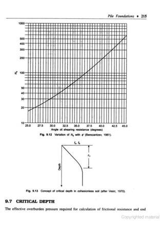
such as Pile Driving Analyzer (PDA) and suitable transducers whic8cr~'}~l~t~hFdd<t!';ii.~

245. Hidden page

246. Hidden page

247. Hidden page

248. 12.6 + 17reory and Prach"ce of Founda#on Design
The building codes provide minimum allowable spacing of piles in a group. I.S. 2911
(pan 1), 1979, suggests the following guidelines for spacing:
(a) For piles bearing on a hard stratum and deriving their strength mainly from
end bearing. the minimum spacing shall be 2.Sd, d being the diameter of the
pile.
(b) For friction piles in clay. the minimum spacing shall be 3d.
(c) For piles driven through loose sand or fill, the minimum spacing may be 2d.
However. the most commonly used spacing is 3d. Figure 9.21 shows some typical pile
groups with different number of piles.
, ..._,A
f.
~~
~
0.87• ·
...
;
rr·-~ ~o"'()'':e:.
t ....... o:
;,
•
.
•
.
4
$
3 piles
:
•
~· t·t·f
'
1
·~·.J!
:
•
•
•
•
'
•0
'
'
6 piles
........0·''
5 pUes
:o
0
0
r····-··---·
~
:O
:o
tt·.t.-f
1
0
0
0
it-1~-f
8 piles
7!llles
-&!-+'
••
~
0
•
9piles
:rr-·-~r-1:
.. -;10
~- · -~J~:.
11 piles
10 piles
(a)
Single rfW for a wall
•
Double
row for a wau
(b)
Fill. 8.21 Tv!>leat pile groups.
Tripfe row for a wall
Copyrighted material

249. Hidden page

250. 228
t
Titeory and Practice of Foundation Design
p
= M rCI
11
Lx;
s
!':!.Jz.
Z.u
On the other side or CG. the reaction is upward, that is, P1 is negative.
P _ ±Ma x, _ ±Mu
Thus.
where
" -
L,x; -
Z.u
P11 = maximum reaction due to moment M11 and
x1 ;::; maximum distance of pile from YY axis.
Similarly, maximum pile reaction due to the moment. MD is given by
P~, =
where.
Thus,
±MuYJ
~
2
~ y"
=
±Mu
t
yy
P_. 1 = maximum reaction due 10 moment Mu and
x1 = maximum distance of pile from XX axis.
I I.
load
V
" 1 M,.y1
pile =P= N±Myy.<, £... x.±
(9.30)
It should be noted here that for large moment on a pile group, the reactions due to
moment may be even greater than the reactions due to the vertical load. In such cases, the
outermost piles on the leeward side of the moment may be subjected to uplift forces.
9 . 13 SETI'LEMENT OF PILE GROUPS
As yet there is no precise method of estimating the settlement of pile groups. The problem
is sti11 approached in an approximate manner.
9.13. 1 Pile Groups in Cohesive SoU
The settlement of a pile group in predominantly cohesive soil is given by the sum of the
immediate or elastic settlement and the long-term consolidation settlement of the subsoil. The
procedure for calculating these settlements are similar to that for raft foundations with
appropriate depth corrections as described in Chapters 7 and 8. However. it is. necessary to
determine the load distribution around a pile group in order to obtain the size and depth of
the equivalent raft from which the settlement is to be determined.
It requires rigorous mathematical analysis, for example, fini te element technique, to
determine the true Slrc$S distribution around a pile group (Poulos and Davis, 1980) but SU<:h
analysis is highly complex and is seldom used in practical design because pile founda1ions. in
any ease arc expected to undergo small settlement. Simplified method of load distribution has
been suggested by Terzahi aod Peck (1962) and Tomlinson (1967, 1977). Accordingly, tOilll
load, Q is assumed to get dispersed from the foundation level at a s lope of 4: I upto the
depth of an imaginary raft at depth 2DJ'3. as shown in Fig. 9.23. Here, the size of the
imaginary rnft becomes (B + D/6)(L + D/6). Thereafter, the load is assumed to get
dispersed at a slope of 2: I into the underlying strata. If the pile group passes through a very
weak strntum to an underlying hard stra1
um, the load is assumed to spread at a slope 4: I on
an equivalent raft a1 a depth 2U3, where Lis the embedment of the pile G'nJ!h
J:rigiT strlltilffi erial

251. Hidden page

252. 230 • Th~ory and Practice of Foundatio11 Design
To know the effective depth of soil below the pile group, the best method is to
determine the. stress increment ratio Aplpfl at different depths and consider the depth of soil
for which llplp > 0. I.
Pile Groups in Cohesionless SoU
9 .13.2
Pile foundations in sand are not expected to undergo appreciable settlement because of the
low compressibility of medium to dense, where piles are usually terminated. Still, if
necessary, the settlement of pile groups in granular soil may be determined by using the same
methods as given for rnft founda tions. The load distribution in the soil and the equivalent
raft concept proposed for cohesive soil may also be adopted to obtain the geometry of the
problem to be solved. Funher, for the methods described in Chapter 7 for foundations on
sand, Schultze and Sherif ( 1973) used case histories to establish a method of predicting the
settlement of foundation on sand. The same method when adopted for pile groups gives
S=
where
Sq.
(9.33)
~ 81 (1 + 0.4~ )
S = settlement coefficient.
q, = average pressure on the equivale.nt raft.
N
= average SPT value over a depth
28 below the foundation level or Ds i f the
depth of cohesionless soil is less than 28,
D1 = depth of equivalent raft, and
8 = width of equivalent raft.
The settlement coefficient. S varies with DJ'B as shown in Fig. 9.24.
10.0· ~-----------~
I
p -
sp
N'·"(1 • 0 .40,18)
D,JB
~
2
D
,
V~/////PP//////////H/////////1'
Reduction factors for
1~8
Dsl
0.1L-'---'--'-.L...I.-...L..-L-l-'-l
0.5
1
2 3 4 5
10
20 30 4050
Breadth, 8 (m)
FJg. 9.24 Setltement coefficient.
s versus
1.5
1.0
0.5
o;s
< 2
1
2
5
100
0.91
0 .76
0.52
0.61
0.72
0.87
0.69
0.43
0.85
0.65
0.39
0.48
DriB (Schultze and Sherif. 1973).
Copyrighted material

253. Pile Foundations • 231
9 . 14 UPLIFT RESISTANCE OF PILES
A straight shaft pile, when subjected to uplift forces, derives its ultimate capacity from
frictional resistance of the pile which can be determjned in the same way as indicated for
piles under compression (see Section 9.7). However. for cyclic loading, skin friction may be
reduced by the degradation of soil strength at the pUe-soH interface under repelitive load. In
particular. for sandy soils. reduction in uplift capacity to SO% of the ultimate skin friction
has been reported (St. John et al., 1983). Even for cohesive soils, Radhakrishnan and Adams
(1973) have observed 30-50% reduction of uplift capacity in short augured piles. Such
reduction in uplift c.apa<:ity has been attributed to long term creep under sustained loading
whereby the strength of the soil reJOches its residual value. As a general rule, a fac tor of
safety of 3-4 on the frictional resistance calculated for compression may be applied to
detennine the uplift capacity of piles. However. it should be noted !bat an upward movement
of only O.S- 1% of the pile diameter is required 10 mobilize the peak frictional resistance.
In case of pile groups, the uplift resistance may be calculated by taking the resistance of
the soil enclosed within the groups. as depicted in Fig. 9.25. for cohesionless soil, an
assumed spreJOd of I :4 from the pile tip to the ground and the weight of soil block enclosed
within lhe group give the frictional resistance. In such cases, Tomlinson suggesL~ a factor of
safety equals to unity against uplift since skin friction around tbe periphery of the group is
ignored. The submerged weight of the soil below tbe ground watef table should be taken.
ttttt
~!.-- Btocl<
Btocl< of sol-
I.s .
L....
of soil
lifted by piles
H
lifted by piles
{b)
(a)
F~. 9.25
Uplift resistance of pie group.
for cohesive soils, the uplift resistance of the block may be obtained by summing up
tbe undrained shearing resistance around the periphery of the block and the weight of soil
enclosed by tbe group as
(9.34)
Q. = 2(L + 8)D1c, + IV
where
L = length of the pile group.
8 = width of the pile group.
D1 = depth of tbc pile group.
c11 :: average undrained shear strengch of the cloy. and
IV = weight of the soil enclosed within tbe block.
A safety factor of 3 should be used to determine the safe uplift capacity of tbe group.
Copyrighted material

254. 232 • T7reory and Practice of Foundation Dtsign
9 . 15 PILES UNDER HORIZONTAL FORCES
·.
Vertical piles can resisc lateral forces to a certain extent depending on the strength
and stiffness of the pile and the soil. According 10 I.S. 2911- 1985, permissible
lateral load of a vertical pile is 2-5% of the permissible vertical load. For greater
horizontal load. addjtional reinforcement is to be provided in the pile or raker piles may
be used.
Ullimate lateral resistance and load-deflection behaviour of a pile under lateral load is a
complex problem of soil-si!Ucture interaction. The lateral load on the pile head is initially
carried by the soil close to the ground surface resulting in elastic defonnation of the soil. As
the load in<:reases. the soil yields and transfers the load to greater depths.
9 . 15.1 Fall1Ue Mecb•ntems
Short and long piles fail under different mechanisms. This subsection brieny discusses these
failure mechanisms.
A s hort rigid pile. unrestnined at the head, tends to rotate or tilt as shown in
Fig. 9.26. and passive resistance develops above and below the point of rotation on opposite
sides of the pile. If the pile head is restrained by a cap. the re will be lateral translation.
In both the cases. the pile will fail when the applied load exceeds the passive resistance of
the soil.
Load
H
,._
I
I
I
I
H
I
I
I
I
L
..e o1
L~--c.n
I
I
I
I
rotation
I
I
I
I
I
I
L-
(a)
( b)
Fig. 9.21 Failure mechanism of rigid pile under hori:zonlal load: (a) free head, (b) ftxed head.
For a long pile, the passive resistan<:e is very large and pile cannot rotate or till. The
lower ponion remains almost vertical due to fixity while the upper part deflectS in flexure.
The pile fails when a plastic .hinge is formed at the point of maximum bending moment,
Fig. 9.27.
As a consequence, a shon pile fails when passive resistanc-e of soil is exceeded
(soil failure) and a long pile fails when the moment
~ap<lcity
is e.ceeded (si!Uctural failure).
Copyrighted material

255. Pil~
1~'/l'illlli'
o
H
Foundations t 233
'!
, If.._
r-- Fracture
L
L
•
(a)
(~)
Fla, 1.21 Fan... , . . , _ , o1 1oog p1o under horiza>tal lood: (a) -
head, (b) -
head.
For development of ultimate · resistance, the lateral movement is generally too large.
Therefore, after c,aJeuJating lhe ultimate resisrancc and dividing by a facror of safety, it is
nec.essary to check that the perrni ..ible deflection or pile head is not excuded.
9 .15.2
SWfDess Factors aDd Subgrade Modulua
The stiffness factors, R and T, of the pile-soil system determine the behaviour of a pile as a
short rigid pile or a long flexible one. These factors depend on the stiffness, £/ or the pile
and the compreosibility of the soil expressed in terms of a soil modulus. The soil modulus
depends on the type of soil, the width of pile, and the dep<h or influence area and is related
to Tert.aghi's modulus or subgrade reaction.
For stiff overconsolidated clay, the soil modulus is assumed to be constant with depth,
and the s tiffness factor is given by
R=
where
~ :~
(9.35)
in units of length
K = K111.S in which K1 is Tenagbi's s ubgrade modulus in kg/m3 or kN/m3 and
D
=diameter of pile.
According to Tenaghi (1955), K 1 is rela1ed to the 'undrained shear strength or the clay as
shQ.wn in Table 9.3.
Tablt 9.3 Values of K1 for different consistencies of clay (after Teru~Jhi. 19SS)
Uncq,ifintd ootnp.
suiT
Very stiff'
Hard
"""''It, q.(lcNim')
100-200
200-400
>400
(kNim'J
R«<tMtnathd, K1
(tN!m')
18-36
36-72
>12
27
S4
>108
R4nse of K1
Copyrighted material

256. 234 • nuwry and Practice of Foundation Design
For soft normally consolidated clays and for granular soils, the soil modulus is assumed
to increase line:trly with depth. For this case. the stiffness factor is given by
T=
where
~ E./
"•
in units of length
(9.36)
n11 = coefficient of modulus variation
= K Dlx, where x is the depth of soil considered.
The "• values for granular soil may be obtained from Table 9.4.
Tablt 9.4
n• (kN/m3) for gnnutar soH (after Terzaghi. 1955)
Typ< of sand
U>ou
Mnlium
TXIrsr
Dry or moi5.t sand
2500
7500
Sub merged sand
1400
5000
20000
12000
For sofl normally consolidaled c lay,
"• = 350 to 750 kN/m3
For son
organic silt,
"• = 150 kN/m3
The criteria for behaviour or a pile as a shon pile or a long pile are related to the embedded
length, L as follows:
Long Pile: L ~ 4T or L ~ 3.5R
Shon Pile: L S 2T or L S 2R
9.15.3 tnttmate Lateral Resistance
The method suggested by Broms (Broms, 1964: Poulos and Davis. 1980) appears to be most
convenient for design. Broms assumed simplified distribution of soil resistance for cohesive
and cohesionless soils and determined the ultimate capacity of short and long piles in tenns
of the flexural rigidity of the pile. The design chans prepared by Broms are given Fig. 9.28
through Fig. 9.31.
In Fig. 9.28, the variation of H./c.d' versus UD (where H. = ultimate horizontBJ load.
c. = undrained shear strength of soil. D = pile dia, L = embedded length) have been plotted
for short piJcs in cohesive soils. Curves for both restrained and unrestrained piJes with
differen t eccentricity ratio have been presented. In Fig. 9.29, the corresponding plots for
shan piles in cohesionless soil with design curves for HjK,J>'rversus UD (K, =coefficient
of passive earth pressure and r= unit weight of soil) are presented. The curves for long piles
in cohesive soil are given in Fig. 9.30. The normalized ultimate lateral resistance, H
Jc..D 1 is
ploued against normali:z.ed yield moment, M,;.,Jc.,D'. Figure 9.31 shows corresponding
curves for cohesionless soil. where normalized ulcimate lateral resistance. H./K,!Yr has been
ploued against normali:z.ed yield moment, M,..1JK,rD'.
..
Copyrighted material

257. Q,.(g)
11"
Pile Foundatioru • 235
-·-pile
Embedment qth. uo
Fig. 1.21 Oulgn chafls for short pleo in coho5Ne ooll (llroms 19M).
Lenglll, LID
Fig. 8.21 Design charts fot Short plies In coheslonleas 8041 (Stems, 19&4).
Copyrighted material

258. ~
• Theory tmd Pro<:tice of Fouru/4tion Design
100
60
40
+;
20
i
I
10
6
•
2
1
3
•
6
10
20
Ulllmollo -
40
100
-:1J
200
men-. U..tc,D'
-
Fig. UO Oooign chor1 lor long piloo in ooheoiYe soil (Broms,
600
19&4~
i; 1000H f
f ·
.
I 10~~~~L-J
"'.
i!'
...1
'
100~-~ ~
~~o~r--------+--------+-~~
Free head
i
I
Copyrighted material

259. Hidden page

260. 238 + Theory and Practice of FoUJI(/Q.tion Design
s,.
A,
-1
0
2
~---~~
1
!;;
1
0
3
•
5
0
~
~~
:::::
2
1
•
2
3
•
0
4::',. · ~
1
2 ...
•
•
3 ~
.... 3
••
,tl
•
10
5
0
1
!;;
2
•
...
3
1,
02 04 06 0.6 10 12
.
. .
r-:-'.
~
y
'l.
~
0
0.2 0.4 0.6 0.8 1.0
0
-L!· ........ ~:4
,. -'l
/'
2 ...
» 'f
•IKo
•
3 ~
•
10
5
5
Fig. 1.32 Pile c:lefJecllon ltld moment In CXJheslcnleu SOit: Elulc anatysis
111- and Mallock (19S6~ Oas (1998)~
, Q1 R3
M1 R2
x,(z) = A, "'E[" + B, E 1
,
I'P
(9.43}
PP
(9.44)
and
wbere A:r, 8'¥, A~. and B'.. are coefficients and R = ~ EPI,IK .
The variation of A~. B'p A;,., and B'. with
z is given in
Fig. 9.33.
8~.
0
-1
-2
1
2
z
3
/
v
3..._,
&"'
0
2
1
~
"'
j. 1
-;:::;-. 2
'.
'
l~ 3
Z..•2
5
•
5
-
8'.
-- a;.
Fig, 1.33 Pile denection and moment in CXIhesive soil: Elastic analysis (0avi$SOO and Gill, 1963),
Copyrighted material

261. Footings and Raft Design • 195
~~~5 )
1!.!> = ( ror Z IB =
6p
-=
p.,
1
;;
1
0.35 x 50.8 = 17.8 kN/m2
= 0.09 < 0. 1
Hen<:e. soil below stratum III is not significant.
33 + 49.8
81 + 37 .5
+ 0.08 x 12 log
33
81
139 + 17.8
+ 006 x 4 1
·
og
139
p, : 0 ,03
X
1•5
X
1Og
= O.Ql8 + 0.158 + 0.012
= 0 .188 m
Deptlvcorrection = 1.0
Rigidity correction = 0.8 _
Pore· pressure correction = 0. 7
I
• (p,),.. = 0.8 X 0.7 X 0. 188 = 0.105 m
Pi = 0.017 + 0.105
=0.122 m = 122 mm < 125 mm
E><amp1e 8.6
, Design of a buoyancy raft foundation for a 4-storey donnitory building with two columns in
each bay, depicted in Fig. 8.25.
I
Depth (m)
0
1
-
0.6ml
Basement
E
..,
3m
I
~
9m
/ I•
•I ',
+A
I
.
Cc/(1 + flo) ' 0 .12
I
I
I
8
Soft organic clay
I c., = 20 k:Nirnl
I
•
J ~/(1 + o0) = 0.15
+B
I
I
I
I
15.5
E
'
7.5
19.5
Soft ore~ day
c_,• 30
'' '
I
+c
'
....
_____ .
I
I
'
I
I
Firm Cf3y
c, = 60 kNtm'
•
I
I
I
I
•
..,
t
@
g
'
4
C,/(1 . . ., • 0.08
N = 30
1
Mediurn sand
~
m
Fig. 8.25 Example 8.6.
Copyrighted material

262. 1% • Theory and Pracriu of Foundmion Desig11
Solution
Size of rnft = 9 m x 90 m
Area of each column bay = 3 m x 9 m = 27 m1
Load in each bay = 2 x 900 = 1800 kN
Gruss foundation pressure
for superstructure q =
1800
2"7
= 67 kN/m1
Assume weight of basement to be 25% of superstructure weight. Thus. q -0 = 17 kNim1
:.
q1,.., = 84 kN/m1
Provide depth of foundation, D1 = 3 m.
q,.. = ql""' - rDI
= 84 - 18 X 3
= 30 kN/m1
•
.
(a) Bearing capacity
Consider 9 m depth below raft
:. c.,
25
=
4.5 + 20
X
X
4.5
= 22.5 kNim2
9
and
= 5( I + 0.2
~)
= 5(1 + 0.2
N,
io)
= 5.2
qult(n) = cllN~
= 22.5
X
5.2 = 117 kN/m2
Fs = ';; = 3.5 which is O.K.
(b) lmmtdiate setllemenl
Consider layers I. II, and III.
q. = 32 kN/m1
8 = 9 m
v = 0.75
lp
= (for UB = 90/9 = 10) = 2.5
30
X
4.5 + 20
X
16.5
8 + 60
X
4
= 32 I<N/m1
Copyrighted material

263. Hidden page

264. 240 • Theory and Practice of Foundalion !H.slgn
I
i
~length.~
Fig. U 5 Oelloctlon ol plio -
9 . 15.5
u.- wmclng lood:
Ccllloolw ooll (Bromo, 19ee).
1.8 . Code Method
(I.S. 2911 (Part 1/Sec. 4)-1984, Amended in 1987)
In this method, a long pile is considered as a cantilever with fixity at some depth below the
ground surface. lbe depth of fixity depends on the relative stiffness of pile and soli,
Fig. 9.36.
2.3
..
3a
~
'
l1
' , "--
1.9
1.7
0
- - - - Fbood heed pile
2.1
- - FrMheadpllo
=
t·m:jm.
.
~..
L
1
.1.
r=
L
------} Forplleoln-and
normally-~
'' '
1.5
0
--- -----}For-in
po-
1.3
0
•
8
L,IR or L,IT
2
Fig.
ue
8
Analysis o1 1a-1 load:
days
10 ..
IS CX>de meltlod.
Copyrighted material

265. Pilt! FoundationJ •
241
Considering lhe pile as on equivalent cantilever. the pile load deOection, y is obtained as
y •
Q(!., + L1 l'
for free head pile
3£,1,
(9.45)
L
d
Q(l., +
=
12£, 1,
for fixed head pile
where Q = latenl IMCI and Lt and It on: as shown in lhe figutt.
The fixed end moment (M,) of lhe equivalent cantile~ is given by
M, = Q(l., + L 1 ). for free ~d}
=Q
!., +
(9.46)
~.,
, for fi xed head
2
The actual rnornent is obtained by opplyln& ttduc:tion factor. as depicted in Fig. 9.37. which
is given by
At •
mCMrt
1.0
-- -- In1---
0.8
E
~
J!
0.6
~
£
0.4
0.2
1
,
7
kL::
1?-
L,
-
For piles
di)'S
- - - F« Clho In """" end
normally toodod days _
0
11~
T
...
1
/
.
L
2
0
•
8
10
12
1.2
-
F0< plloo In pertoodld ctayo
-- - FO< pilot In Nnd onc1 normolly -
L.--
0.8
v
----V'
0.5
-
1--L~G~
T'~
1
0
days
tO
;I {
tS
20
2.5
LvR or Lv T
(b)
Flo.
t.n ecr-. ....., "" tonv p1es ~s 21111~
v

266. Hidden page

267. Hidden page

268. Hidden page

269. Pile Foundations • 245
A semi-empirical method of estimating the negative drag based on the one described by
Terzaghi and Peck (1967) has been suggested by Nayak (1967). It can be done through the
fo llowing steps:
1. Estimate the length of pile over which negative skin friction develops.
2 . E.~timate the positive skin friction over that length.
3. Multiply the value obtained in (2) by a fac tor to obtain dragdown. This factor
depends on the cause of soil movement and may be taken as a value varying over
0.6-0.8.
4. Estimate the ultimate pile capacity, Q..p as consisting of point bearing and shaft
re.~istance over the length where there is no negative skin jricrio11.
5. Calculate factor of safety, F from
·
F =
Q.P
(Q + Q.,)
where
(9.51)
Q = structural load on pile and
Q,, = downdrog force on the pile.
In a pile group. the total downdrag force on the group. Q., is the minimum of the following
values.
·
(9.52)
Q., = NQ.,
and
(9.53)
Q"·' = yL"P
the weight or soil enclosed with the pile groups,
where
N = no. of piles in the group,
r = unit weight of soil.
L,. = length over which negative friction develops, and
P = perimeter of the group.
Poulos and Davis (1980) have described a method based on elas1ic lheory. wilh
allowance for pile-soil slip, to estim:ue downdrag force. ln this method, the dependence or
downdrag on the settlement of the soil can be included, rother than assuming that sufficient
soiJ movement occurs to mobilize the full adhesion along the pile shaft. Based on a study of
the various parameters responsible for negative skin friction, the authors have presented
charts which can be used very con..,eniently to calcul::ue downdrag force.
9 . 17 TESTING OF PILES
Recent trends in foundation design follow the use of large diameter, high capacity piles fo r
supporting heavy s tructural loads. Till the early sixties, driven piles of diameter upto
SOO mm were nonnally in use in India. These ptles would have safe load capacity upto
100 lonnes depending on the deplh of pile and s ubsoil condition. Wilh 1 coming of bored
he
cast·in..:situ systems, large diameter piles are now common and typical 1500 mm diameter
piles with safe capacity of 500 tonnes or more have frequently been used in recent years.
This obviously necessiunes o strict quality control in the installation of the pile so chat each
pile carries the des ign load with certainty.
Copyrighted material

270. 246 +
17u~ory
and Practice of Founda.tiou Design
9 .1 7. 1 Purpose of Pile Testing
ln bored c- st-in-situ piles. a vertical hole is made into the soil by augering and the
a
same is stabilized by casing or drillin_ mud. A reinforcement cage is insencd and lhe
g
hole is filled with concrete by the tremie method. The entire operation being directed from
the ground. uncertainties remajn as to the condition of the soil at the pile tip and the
integrity of the oon<:rete in the pile shaft. The purpose of pile testing is, therefore~ to
determine
(a) whether the pile tip has reached firm st'ratum or it rests on loose soil at the bottom
of the hole.
(b) whether the concreting of the pile shaft has been done properly and without any
discontinuity. and
(c) whether the load c.arrying capacity of the pile has been correctly assessed.
There is no readily available method of checking tbe condition of the soil at the pile tip
prior to concreting. Normally, at the end of boring. reverse circulation is done to remove all
debris from the bottom of the hole and the depth is finally obtained from the length of the
tremie pipe and the depth of boring. Even then. un<:ettainities remain about the possible
existence of any thin layer of loose soil at the pile rip.
9 .17.2
causes of Defect in Piles
Defects in pile shaft normally occur in the form of unfilled voids which cause discontinuity
·in the pile shaft. Major causes of such defects have been listed by Tomlinson (1981) as
Encrustation of hardened concrete on the inside of the casing which may cause the
concrete to be lifted a~ the casing is withdrawn.
(b) The falling concrete which may arch across the casing or between the casing and
(a)
the reinforcement.
(c) Falling concrete may ger jammed between the reinforcing bars and not move
towards the borehole wall.
(d) Clay lumps may fall into the hole as the concrete is placed.
(e) Soft or loose soil may squeeze into the pile shaft from the bottom of the lining.
Most of these defects can be minimized. if not eliminated. by having the inside of the casing
properly c leaned. using a high slump concrete and by avoiding conjestion of reinforcing bars.
Also, proper care needs to be taken in lifting the casing while concreting, particularly in
unstable soils.
9 .17.3
lnte~ty
Testing
Often excavations for pile caps show defective construction near the pile head. Similar
defects may be there at greater depth also. Therefore. integrity testing is done to check the
soundness of the pile shaft after installation. The following methods of integrity testing of
piles are generally available (Weltman. 1980; Robertson, 1982)
Copyrighted material

271. Pi/~
(a)
(b)
(c)
(d)
(e)
(f)
Foundatimu + 247
Excavation surrounding the pile shaft
Exploratory boring through the pile shaft
Acoustic tesu
!Udiometric tosts
Dynamic response of pile
Load test
Excovarion around the pile shaft Is only possible for shallow depths. It is hardly
conceivable that a deep pile can be fully exposed for visual inspection. However. shon piles
or limited length or pile near the ground surfoce ClU1 be examined thoroughly.
Drilling/l>ori~ rhro,gh the pile shaft is pclUlble through IIIJe diame~er piles. Cores of
concrete can be examined for soundness and they can be tested to determine their
compressive strength. Even a TV Camen may be lowered onto the hole to look for cavities
and honeycombs.
Various mdit»Mtric 1111d aroustic ttsts ate also done in drilled holes. Pairs of ducts m:
made in the pile shaft at the time of concretin& and suitable scanning devices are inuotluecd
to scan the concrete between the ducts. However. these require specialized equipment. Sonic
inu:grity testing is one sueh lC$1 which Is gtlnin& popularity.
S4!ismic and dynamic response ttsts o.re extensively done because of their simplicity and
adaptability. No hole is required to be made in the pile shaft. In the seismic method. a
weight is dropped on the pile head and the time for return of the seismic wave after
reflection from the toe is measured. In the dynomic,: response method. an eleclfodynamic
vibrator is mounted on the pile head to apply o constant amplitude stress wave at the pile top
and the response or the pile Is seen through an ~cillogr•ph or digital indicator. Various types
or pile diagnostic syStems/pile d.rivlng analyzers are now commcrc:iruly available to facilitate
such testing.
Load rest is the most direct method or determining the c11p:w:ity of the pile. While other
methods of integrity testing determine primarily the soundness or the concrete, the load test
gives an integrated method or determining both the JOundncss of the conc rete and the
response of the soil under load. It also permits an evaluation of the load carrying capacity of
the pile on the basis of soil te$ponse. The next section discusses lood tcsl on piles in a much
greater depth.
9 . 18 LOAD TEST ON PILES
Initial and routine load tests are commonly undenaken in oil ptling work in Indio. The
basic purpose of an inidal load test is 10 obtain the failure load of a pile and then to
determine the design load by applyina a faetor of safety. However. for IIIJer diameter piles.
this means applying a very heavy load on the ptle to take it to foilure. Rooti1te rests are
carried out on woridn& piles lo serve u 1 proof test to ensure that the behaviour of pile is
satisfactory. This test is carried out on a limited number of working ptles as a measure of
quality control.

272. Hidden page

273. Pile Foundations • 249
(c) The load at which the settlement of the pile head is equal to 10% of the pile
diameter.
Pile load (kN)
0
0
.......
1000
2000
3000
.........
" ~ 1•
'
r60
-
b
Fig. t.43 LOad versus &ettlement relationship from pile teal
According to IS 29-11- 1985. the safe load from initial load test is taken as the least of
the following:
(a) Two third of the load at whieh gross settlement is 12 mm or
(b) 50% of the fi nal load at which gross setllement becomes 1/IOth of the pile
diameter.
The ultimate load obtained by these methods for the pile test data, as depicted through
Fig. 9.43, is shown in Table 9.5.
Table 9.5
Pile cap:~city from lood test (Fia;. 9.43)
MttiJod
UllimoU l(JI((iJ (k N)
Sa/~
lood (k.N) FS • 2
Double t3tlgent (on arithmetic ploc:)
Double taosent (on log-log ploc)
t900
t320
950
Seulcmcnt 1
0% pile diameter
2300
tl50
t300
870
II SO
~
I. S. /985
213
lo3CI at 12 mm sculemc:nt
so~ o( load a1 sculemenl o( 10% pile diameter
gTOS$
2300
In routine load test. the pile is considered to be safe if the gross settlement under 1.5
times the working load is not greater than 12 mm. However. this criterion of 12 mm gross
settJement should be related to the pile diameter particularly a large diameter piles.
Maintained load test is very time consuming. Also. some amount of consolidation and
creep may take place during the test. So, it may be difficult to correlate the test results with
undrained shear strength data obtained from laboratory tests.
9.18.3 Constant Rate of Penetration (CRP) Test
This is a short duration test in which the load is applied at a cons1ant rate of strain till the
pile fails. The rate of strain depends on the type of soil. A common nne i$ 0.75 mmlmil1 for
,
Gopynghteo m;nenal

274. Hidden page

275. Pil~
Foundatio11s •
251
9.18.4 Pile Driving Analyzer
Meo.surcment of stress waves in piles has led to the development of a new and versatile
equipment for testing the integrity of piles and predicting pile capacity. Different types of
pile driving analyzers (PDA) arc now commercially available. These arc essentially based on
the propagation of stress waves down and up the length of the pile while the boundary values
applied at the pile top are used as inputs for the wave equation analysis. The commonly
available pile driving analyzers arc capable of determining the
(a) pile bearing capacity,
(b) maximum compressible and tensile stresses.
(c) maximum pile top movement, velocity. and acceleration and
(d) pile integrity.
For interpretation of data. a wave equation analysis programme is developed and fed
into the system. For example, PWDWAP (Tan et al ., 1987) uses a model of the pile as
discrete line elementS and lhc soil as a system of elasto--plastic springs and viscous dashpotS.
The programme uses an implicit Newmark integration analysis and displays the measured and
predicted responses on a computer screen and presents the data in convenient worksheet
format. Tan et al. {1987) present five case histories of piles in residua! soil and one in
alluvium formation. The pile capacities that predicted the Hiley's formula were compared
with the results of PDA and load teSts data (refer Table 9.6).
Table 9.6 Summary of pile capacities (Tan ec
S.No.
Slu of pUtt
U..s•h
(mm)
(ml
Design load
(m)
at.. 1987)
Hil~
Ullimatt- Load
PDA
Lood f~M
formula (I)
5.
Residual Soil
Cone. 280 x 280
Cone. 325 x 3 25
Stc<t 3S6 X 368
Sted 356 X 368
St..J 356 X 368
6.
Slecl 35.6 x 368
I.
2.
3.
4.
(I)
(!)
272
360
310
250
400
268
380
390
283
390
372
330
2.1. t
25.6
40.8
29.4
28.0
t20
120
t20
220
355
368
352
427
11.0
110
252
93
liS
Alluvium
A field test with POA is shown in Fig. 9.45. Major defects such as crocks. soil
incursions, necking, and changes in cross section are easily detected using this cesl. For
complete pile driving analysis, two specially designed combined acceleration and strain
transducers are mounted on the side of the pile near the pile top. During driving of piles,
signals obta.i ncd through the mounted ·transducers are passed on to the signal conditioning
subsystem for processing and finally to the computer. The processed signal for each blow is
stored in o hard disc memory and displayed on the computer screen. After pile driving. a full
record of all relevant parameters are ovailable with respect to the number of blows as well as
depth. Typical test data obtained for structuraJiy sound piles and piles with discontinuity are
shown in fig. 9.45.
Copyrighted material

276. 252 • Theory and Practice of Foundation Design
Blow
Ret'lex of pile toe
=~ +-·!- r1
5.4 cm/s 0
2
4
i l l-l-H I :~:
6
8
10 -
12
14
16
18
20
Structurally sound pilo
Crackldecrease In
77
.
aoss secllon
-tr-H Y I I I I I
l
4.5 m
Pile 1111 necking
Increase In cros.s.secOOn
5.6m
0
1
2
3
Fig. 9.4S
•
5
6
7
8
9
m
10
POA results cast-In--situ concrete plies.
Example 9. 1
A closed ended steel pipe pile, 30 em in diamerer and 20 m long is driven to a sand deposit
with cut off at ground level. The depth~wise variation of N and
9
values is given in
Fig. 9.46. The waler table is 3 m below ground level. Compute the ultimare load capacity of
!he pile based on soil support, using
H (Biows/30cm)-+10
(m)
20 30
0~----~----~~~~~~~~
•
I
--------- ----------7·
27.6 kl<lrn' _.,._
''
2
3 : ----- -·
IH• S
-...;::~
f---
Skin friction :
I
-------- --------~---39 kNrm2
~
N •
--- .......
16
251- ---- --------- - ------------- 4 N
Fig. 9.46
Vartallon
of
•
22
N and ~ with depth.
Copyrighted material

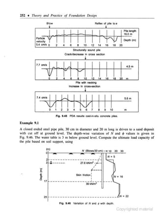
277. Pile Foundar;ons • 253
(i) N value.
(ii) Overturden pressure considering c ritical depth.
Take effective unit, t' =- 1.73 tlm3 above water table. and 0.73 rJmJ below water table.
So/uJion
(i) Using N value
Average N along pile shaft. N., = [(5 • 2) + (16 • 15) + (22 • 3.6)Y20.6 = 15.98
= 16 (upco 20 below tip)
N value below tip = 22
Using Eq. (9.19)
Q• = 4NAp + N., A1
6
= 4 X 22 X 0 .785 X (0.3)2 + (16/6) 3.14 X 0.3
=62.22 + 50.24 = 112.41 = 112 I = 1120 kN
(ii) Considering critical depth for overburden
For medium sand, ~ID :: 20, z~ = 6 m, N,
Fig. 9. 12.
For driven steel pile, lAke K, = 1.5, ;.. =
0 -3 m: '-•
3- 20 m :
Also,
Q.
~
..
= 45,
X
20
using Berez.antzev's curve.
0. 7~'
= 0.7;'
X
=0.74>' •
28° = !9.50°
32°
=22.5°
= f. + A ,
LA, ,q
f., = K,yD 1An 19.5° = 1.5 x 17.3 x 3 x can 19.50° = 27.6 kN/m2
1
/,, = K,y•o1 can 22.5°
= 1.5(17.3 x 3 + 7.3 x 1.5) tan 22.5°
= 39.0 t/m2
.
_LA,f. =
1f X
0.3[ 3 X
~7.6 + Je7.6/ 39) + (14
X
39)]
= 1f X 0.3(41.4 + 99.9 + 546)
= 647 kN
and
A9 q,
= " •
°·
,
3
• ( y' D1Nq)
4
2
1f • 0 .3
:
{17.3
4
= 559 kN
X
3 + 7.3
X
J7)
X
45
Q. = 647 + 559 = 1206 kN
Copyrighted material

278. 254 + Theory mu/ Practice of Foundation Design
E•amplt 9.2
Determine the safe load of a group of 9 driven c.ast-in-situ piles, 40 em in diameter, 15 m
long. installed in a cohesive deposit. as shown in Fig. 9.47. The cut off level is 1.5 m below
ground level and the spacing of piles 1.2 m.
}
-
0
c,(l<Nht!')
50
100
oe.icxa ted 111m day
%50kNhn'
Sofi organk: clay
25 kNim'
2.5
g
i
8
13
I ......._
)
15 m
)
Stiff day
100 k
Fig. 9 ..(7 Group of plies ln a cohesive deposit
Solution
Individual pile actictJ
Capacity of • single pile: Q. = Qf + Q,
Taking adhesion factors as follows:
c, (kN/m2)
50
25
100
Qf = 3.1 4
0.4(0.9
X
a
0.9
1.0
X
50
X
9
X
I + 1.0
0.45
X
25
X
10.5 + 0.45
X
100
X
3.5)
= 584.2 kN
Qp = 0.785
X
(0.4i
X
100 = 113 kN (where N, = 9.0)
Q. =584+ 113=697
Q.u = 69712.5 = 280 kN
Safe capacity of 9 piles = 9 x 280 = 2520 kN
Copyrighted material

279. Pitt FormdntiOJIS • 255
Block actio11 (Fig. 9.48)
Depth tm)
,_,
0
1.5
,_,
roi<N.m'
2.5
I
I
I
I
I
I
I
I
I
I
I
I
I
I
I
I
251<N.m'l
I
I
I
I
I
13.0
I
1.2m
1.2m
0.3m
1-"
I
I
I
1001<N.m'l
-.- --- -
I
16.5
1-r.
0.3m
Fig. 9.48 8IOCk
Q.,l
= 2(2.4 + 2.4)(50
X
I + 25
X
action.
10.5 + 100
X
3.5) + (2.4
X
2.4
X
9
X
100)
= 6360 + 5184
= 11.544 kN
Q.,1 =
1
;s;
4
= 4600 kN. which is greater than 2520 kN
Hence, safe capacity of pile group = 2520 kN.
Example 9.3
A mu.ltistoreyed building is to be constructed at a site whose subsoil profile and propenies
are shown in Fig. 9.49. It has been decided to suppon the building on pile foundation. with
cut-off level at 2 m below G.L. Compute the safe load of 25 m long bored piles of 650 mm,
750 mm. and I m diameter. Assume ground water table at ground level and average unit
weight, y = 19 kNim'.
Depth (m)
00
Firm browni-Sh gtey silty day
c.. • •o kNII'nl
Gtey/dark grey silty day
Cu
Firm bluish grey silty day
Cv. 80 kNim2
Silty fine dense sand
Cut-off
N = 40
6
= 20 kNfnY
18
22
Fig. 9.49 Subsoil profile
for
Example 9.3.
Copyrighted material

280. 256
t
111e0ry and Practice of Foundation Desig11
O =
wh
L A,
L. AI/~+ APqP
= lrD (4
X
1.0
40 + 12
X
X
1.0
X
20 + 4
X
0 .55
X
80)
= 1rD(576)
= 1810 D
(Neglect skin friction in sand)
Taking critical depth, .,_ = 20 D = 20 x. 0.75 = 15 m
2
Apqp = : D (9.0 x 200)50
=7060£>'
Pile dia.
(mm)
QJ(kN)
Q,(kN)
Q,n(kN)
Q,u(kN)
(FS = 2.5)
600
750
1000
1086
1357
1810
1524
2978
7060
2610
4330
8870
1050
1730
3550
(Not~: There is some uncenainty O'cr the choice of aitical depth in piles that penetrate through cohesive soil
into sand. If the critical depch is not considered and fuJI overburden is taken. end bearing in sand will increase
appt<eiobly.l
Therefore. 750 mm diameter piles with
Q.,, = 1700 kN arc used.
Example 9.4
A typical column of the multistoreyed building in Example 9.3 is subjected to the following
loads at ground level.
Vertical load V (kN)
DL
5500
LL
760
Mu (kNm)
DL + LL
123.5
SL
657
M11 (kNm)
DL + LL
115.2
SL
SL
985
& se shear
H.(kN) H ,(kN)
SL
380
SL
Using 750 mm diameter bored cast~in-situ piles (safe capacity ns found in Example 9.3).
design a suitable pile group for the column. Also detennine the moment due to horizontal
load for which the section shoold be designed.
Solution
Safe bearing of 750 mm diamecer pile, 22 m long, with cuH>ff at 2 m below G.L. is 1700 kN.
Considering the nature of loading. a 4-pile group (as shown in Fig. 9.50) is chosen.
Pile cap = 3.3 x 3.3 = 10.9 m'
Weight of cap. pedestal. and soil upto G.L. " 10.9 x 20 = 218 kN
1
l,
= ' · = (4 x 1.125)
'
1.125
= 4 _ m'
_
5
Copyrighted material

281. Pile Fou"dotions • 257
(a)
DL + U Condition
i:V =
5500 + 700 + 218 = 6478 kN
M,.
= 123.5 kNm
Myy
= 115.2
kNrn
Maximum load in pile. P
(b)
=647.8/4 + (123.5 + 115.2)145 = 1672.5 kN >
1670 kN.
(Marginal overloading on one pile may be accepted.)
DL + U + SL Co11dition
:!:V = 6478 + 657 = 7135 kN
M., = 123.5 kNm, MTI = 115.2 + 985 = 1100.2.
H,
= 380 kN
.,
125
Load perp1e, p - -7135 • 123.5 ... 45 ... 110 .2 - 1845 kN (<.
-
4
4.5
)C
1700 = 2 125 kN)
(c) Horizontal load
.,
H per P l C
380
= - = 95 kN
4
Maximum Moment on Pile Section
(i)
Using IS Code (IS 2911, Part I, Sec 4, 1984 wilh Amendment in 1987)
Stiffness Factor.
R =
~( Ek:e)
E, = 2 x llf t/m2
1, = (x/64) x (0.75)4 = 0.015 m'
K 2 = 48.8 from code
R = • ( 2 x I06 x " x (0. 75)' ) = 504 em = 5.04 m
64 X 48.8
.
Embedded length. L, = 20 m. L 1 = 0, and L1/R = 0
Using the curve for fixed headed pile in prcloaded clay,
L
...L = 1.6
R
..
Depth of fix ity, Lt
= 1.6 x 5.04 = 8.1
m
Ca'ltilcvcr momcnj, M1 = H(O + f..t) /2 = (95 x 8.1)/2 = 466 kNm.
Corrected moment. M = mM1
Using appropriate curve from code, m = 0.7
:.
Design moment = 0.7 x 466 = 326 kNm.
Copyrighted material

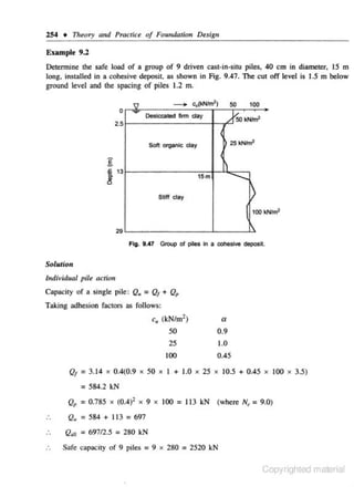
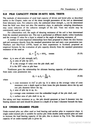
282. 258 • Theory nnd Practice of Foundaticll Design
Example 9.5
Compute the long tenn ~ulement of the pile group considered in Example 9.2.
The load on the pile c-ap is assumed to spread at a slope of 4 horizontal to I vertical
upto the level of 213 pile length from the top. and then at slope of 2 vertical to 1 horizontal
to a depth of 12 m below that level, which is about 1.5 times the width of equivalent
imaginary footing.
Solution
Two points A and 8 arc considered at the mid point of the relevant strata beneath the
imaginary footing. Water table is assumed to be at G.L.
At A.
Po = 12.25 x 9 = 110 kNim1
fl.p
At B,
= 25201(8.2)2 = 37.4 kN/m2
6, = 0.10 x 150 x logto [(110 + 37.4)1110)] = 1.9 em
Po = 19 x 9 = 171 kNim2
tJ.p =' 25201(12.2
62 =
X
12.2)2 = 10.2 kN/m2
x 1200 x lo&to [(171 + 10.4)1171)] = 2.46 em
:. Total settlement = 1.9 + 2.46 = 4.36 em
0.08
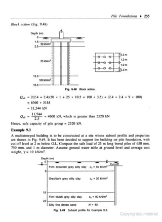
Example 9.6
RCC bored piles, 1000 mm diameter x 20 m long are proposed to be used for a flyover
passing over a canal bed with predominantly river channel deposits, as depicted in Fig. 9.50.
OMC method of boring is adopted and steel liners would be u~d to a depth of at least 15 m
below G.L. Design the safe pile capacity.
N (BiowS/30 em)
0
0
3
•
-
10
--
20
30
40
- :'off-- -,
~
Cut
~N
= 20
10
Brownl$h
medium 10
sand
£
2'
20
0
30
Greyish brown
stiff clay
c., • 100 k.Nim2
40
I
Fig. 9.50 RCC bored plies for Example 9.6.
Copyrighted material

283. Pile Fou,dations • l59
Solution
Here, skin friction will develop between the liner and the soil.
Hence, take K,
= 1.0, 6 =0.7f = 0.7 x
End bearing: Consider reduction of
Q..
Take
t.,
f
34
= 23•
value for bored piles =
f = 36 -
3 = 33°
= LA,!,+ A,q,
= lSD = IS m
/ , = 1.0 x 8 xI S x mn 23° = 51 kN/m2
N• = 43
Q/ =
l.O>r (1/2(5 1 X IS + S X 5 1))
= 1600 kN
Q = 7rl4 (1) 2(8 x IS X 43) = 3950 kN
,
Q. = 1600 + 3950 = 5950
QoJJ =
5950
2.5
• 51 •Nim'
-1 o
- 20 ' - - - . . . J
= 2380 kN "' 2300 kN
Example 9.7
If !he pile in Example 9.6 is laken down to 28 m below cut·off, what will be safe capacity?
Solution
Q. = Q,+Q,
Q/ =
1r X
1.0
X
(5 1
X
15 + 51
X
10 + 0.5
X
100
X
3)
= 3270 kN
Qp = Jr/4(1 )2
X
9
X
100
= 700 kN
Q. = 3270 + 700
= 3970 kN
3970
= 1590 kN ., 1600 kN
2.5
Q. 11 = -
[Note that increasing the pile length increases frictional resistance but there i.s major
reduction end bearing also.)
Example 9.8
A foot bridge having !he main trestle consisting of steel columns (refer Fig. 9.51(a)) is to be
founded in the subsoil shown in Fig. 9.5l(b). Design a suitable pile group for the trestle
foundation.
Copyrighted material

284. 260 • Theory and Practlce of FouudaHon Design
Depth (m)
0
Top sol: Rubbish/day/Brickbats and so on.
140kN
N•6
4
'
I
6.5
5
N•6 Btownish grey sandy silt v.ilh ctay binder.
N• •
I
I
I
I
I
,3
,6
4m
Pile$
I
I
I
N •
N •
0.5
f¥8Y Clayey silt with tine sand
y= 18 kN/ms, Cu = 35 kNfm2
Bt~ish
Gtey/dal1t grey silty day with
decompomsed wood.
r= 17 kNim3
C11 = 25 kN.ffn2
silty day Ytflh kankar.
12 Bluish grey 3
r • 19 kNim • c;, • 65 kN!m2
16
Monied brown silty day.
r = 19 kNim3, tv = 10 kN!m2
22
N
4.0
....
Yellowish/greyish brown silty day with
kanlcar and occasional sand ten
- of
End
5.0
= 25
borehole
(a)
(b)
Fig. 1.51 (a) Main mile COI..,.,s and (b) subsoil
IYPt tor
~·
9.8.
SoiMtion
Pile copaciry
Pile djameter = SOO mm
Depth ~ 18 m/24 m
Cut·Off level
~
I m below ground level
Pile tip at 18 m below ground level
Q... per pile ~ L.A1J, + A,q,
~
~
Uplift per pile
0.5/t (J4Q + 200 + 136 + 84) + (0.2
~
Q,1 per pile
1
0.5lr(4 X 35 X 1.0 + 8
+ lr/4(0.5)2 (9 X 70)
879 + 126 ~ 1005 kN
1005
= 3 (FS) =333 kN
~
879
T
~
293 kN
~
X
25
X
1.0 + 3
X
X
65
X
0.7 + 2
X
70
X
0.6)
630)
,. 300 kN
250 kN
Copyrighted material

285. Hidden page

286. 262 + 111eory and Practice of Foundation De. ign
s
·~
St1uness f actor,
T --
-
.{El
K!
K
~
l
2
X
106
-
4
;r/64(0.5)
60
X
= ~ 102.2 = 2.52 m
Slorm • Impact
140
4
Rigid cap
150
4 =n.skN
---- ~
-"""'!'~------- +
c;,
= 35 ltN!m2
Pile 0.5 m dia
As pile deplh
= 18 m > 4T. Hence, it
!:!,__ =
c,B'
is a long elastic pile and we use Brom's method.
35
= 4.0
35 x (0.5)2
Considering restrained pile
..
-
M,
C11 8 3
= 5, which
M. = 5
X
35
X
gives
(O.S)'
= 21.8 kNm
Berczantzev. V.G.. V. Khristoforov. and V. Golubkov (1961 ). Load Bearing Capacily and
Deformation of Piled Fou11dations, Proc. Slh Int. Conf. on SMFE, Vol. 2, pp. 11- 15.
Birmingham, P. and M. James (1989), An Innovative Approach to Load Testing of Higlr
Capacily Piles, Proceedings of the International Conference on Piling and Deep
Foundations, London, Balkema, Roterdam, 1989.
Bishop. A.W. (I 966). Sixth Rankine Lecture: The Suength of Soils as Engineering
Materials, Georec/mique, Vol. 16, pp. 89-1 30.
Bowles, J.E. (1968), Formdcaio" Jbialysis and Design, McGrnw-Hill [nc., New York.
Copyrighted material

287. Pile Foundations • U3
Bowles, J.E. (1974), Analytical and Complllu Methods in Foundation Engineering.
McGraw-Hill, New York.
Broms, B.B. and J.O. Silbenn.an (1964), Skin Friction Resistance for PUes in Cohesionless
Soils, Sols-Soils, pp. 10-33.
Broms, B.B. ( 1966), Methods of Calculating the Ultimate Bearing Capacity of Piles-<>
sunurwry. Sols-Soiis, pp. 18-19: 21-32.
Broms. B.B. and L. Hill (1973), Pile Foundatioru for Kuwait Towus, Proc. 8th Int. Conf.
on SMFE. Moscow, Vol. 2-1, pp. 33-,;18.
Burland, J.B. (1973), Shaft Friction of Piles in Cia~ simple .fundamental approach,
Ground Engineering, Vol. 6, No. 3, pp. 30-42.
Cooke, R.W. and G. Price (1973), Strains and Displacements Around Friction Piles,
8th Int. Conf. on SMFE. Moscow, Vol. 2-1, pp. 53-«l.
Proc·
Das, B.M. (1998), Principles of Foundation Englnuring, PWS Publishing, California, USA.
Davisson, M.T. and H.L. Gill (1963), Laterally Loaded Piles in a Layered Soil System,
Jou.m al of tht Soil Muhanics and Foundtl.tion~ Division, American Society of Civil
Engineers, Vol. 89, No. SM3, pp. 63-94.
De Beer, E.E. (1970). Experimental Detennination of the Shape Factors and Bearing
Capacity Factors of Sand, Geotechnkple, Vol. 20. No. 4, pp. 387-411.
Aaate, K. (1972), Effects of Pile Driving in Clays, Canadian Geotechnical Journal, Vol. 9.
No. I.
Hanna, T.H. and R.H.S. Tan (1973), The Behavior of Long Piles Under Compressive Loads
in Sand, Canadian Geotechnical Joumat Vol. 10, No. 3: pp. 311-340.
Janbu, N. (1953), An Energy Analysis of Pile Driving with the Use of Dimensionless
Parameters, Norwegian Qe()(echnical Institute, Oslo, Publication No. 3.
IS 2911 (1979)--Code of Practice for Design of Pile Foundations. Bureau of Indian
Standards, New Delhi.
Kerisel, 1. (1961), Foundations Profondes en Milieu Sableux, Proc. 5th Int. Conf. oo SMFE,
Vol. 2: pp. 73-83.
Marsland, A. (1971), Shear Stwogth of Fissured Clay. Stress·Stroin Behavior of Soils, T.G.
Foulis, pp. 59~8.
McClelland, B. (1974), Design of Deep Penetnltion Piles for Ocean Structures. Journal of the
Geotechnical Engineering Division, American Society of Civil En.gineers. Vol. 100,
No. GT7, pp. 709-747.
Meyerhof, G.G. (1959), Compaction of Sands and Bearing Capacity of Piles, ASCE, Journal
of Soil Mechanics and Foundation Division, SM6, pp. 1-29.
Meyerhof.·G.G. and L.J. Murdock (1953), An lnvestigation of the Bearing Capacity of Some
Bored and Driven Piles in London Clay, Geottchniqut, Vol. 3: p. 267.
Meyerhof, G.G. ( 1976), Bearing Capacity and Settlement of Pile Foundations, Journal,
Geotechnical Engineering Division. ASCE, Vol. 88, SM4: pp. 32-67.
Copyrighted material

288. 264 • Theory and Practice of Foundation Design
Nordlund, R.L. ( 1969). Bearing Capacity of Piles in Cohesionless Soil, Journal of Soil
Mechanics and Foundation, ASCE. Vol. S9, No. SM3, pp. 1-35.
Poulos, H.G. and E.H. Davis (1980), Pile Foundatior1.1 Analysis and Design, John Wiley and
Sons. New Yorlc.
Radhakrishnan, H.S . and 1.1. Adams (1973), Long-term Uplift Capacity of Augured Footings
in Fissured Clays, Canadian Geottchnical Journal, Vol. 10, No. 4, pp. 647-652.
Rees, L.C. and H. Matlock ( 1956), Non-dimensional Solutions for Laterally Loaded Pil.s
with Soil Modulus AJsumed Proportional to Depth, Sib Texa.< Conf. on SMFE, Special
Publication No. 29, University of Texas. '
Schultze, E. and G. Sherif (I 973), Prediction of Selll•ment from Evaluated Selllement
Observatwns for Sand, Proc. Sib Int. Conf. on SMFE, Moscow, Vol. I, p. 225.
Sltempton, A.W. (194S), The f 2 ·o Analysis of Stability and its Theoretical Basi.r, Proc. 2nd ·
Int. Conf. on SMFE. Rotterdam, Vol. 2.
Skempton, A.W. (195 1), The Bearing Capacity of Clays, Building Research Congress,
England.
Sltempton, A.W. (1959), Cast in-situ Bored Piles in London Clay, Geotechniqu•, Vol. 9,
No. 4, pp. I 53-173.
Skempton, A.W. and P. La Rochelle (1955), The Bradwell Ship: A shon term failure: in
London Clay, Geotechnique, Vol. 15, No. 3.
Skempton, A.W. and R.D. Nonliey (1952), The Sensitivity of Clays, Geotechnique, Vol. 3.
No. I , pp. 40-5 I.
Smith, E.A.L. (1960), Pile Driving Analysis by the Wave Equation, Journal on Soil
Mechanics and Foundation Division, ASCE, Vol. 86, SM4: pp. 35-61.
Sliwinski, Z. and W.G.K. A eming ( 1974), Practical Consideratio11s Affecting the
Performance of Diaphragm Walls, Proc. Conference on diaphragm walls and anchors,
ICE. London, pp. 1-10.
Tenaghi, K. ( 1942), Discussion on the Progress Repon of rite Committee on the Beanirg
Value of Pile Foundations, Proc. ASCE, Vol. 68: pp. 311-323.
Terz.agbi, K. (1943). Theoretical Soil Mechanics, John Wiley and Sons Lid., p. 510.
Terz.agbi, K. (1955), Evaluation of Coefficient of Subgrade Reaction, Geotechnique, Vol. 5:
p. 297.
Terz.aghi, K. and R.B. Peck (1967), Soil Mechanics in Enginuring Practice, 2nd ed., John
Wiley and Sons, New York.
Thorburn, S. and R.S.L. Mac Vicar ( 1970), Dis.:ussion, Conf. on Behaviour of Piles, ICE,
London, p. 54.
Tomlinson, M.J. (1965), Foundation Design and Construction, 2nd ed., Pitman, London.
Tomlinson, MJ. (1977), Pile Design and Construction Practices, lst ed., Viewpoint
Publications, London.
Copyrighted material

289. Pile Fmmdallons • 265
Tomlinson, M.J. (1981). Pile Design and Constmction Pmctices, 4th ed.. E ond F N Spon,
London.
Touma. F.T. and L.C. Reese (.1974), Behaviour of Bored Piles in Sond. Joumal on
Geoteclmicnl Enginuring Division, ASCE. Vol. 100. No. GT7: pp. 749-761.
Vargas, M. ( 1948), Building S<ttlement Obsm.·atlons in Sao Pnuw, Proc. 2nd lnt Conf. on
SMFE. Rouerdam, Vol. 4, p. 13.
Vesic. A.S. ( 1967), A Snrdy of Bearing Capacity of Deep Formdatio11s, Final Rcpon, Project
B-189, School of Civil Engineering. Georgia Institute of Technology, Atlanta.
Vcsic. A.S. (1975), Principles of Pile Foundation Design, Duke U niversity. School of
Engineering, Soil Mechanics. Series No. 38.
Vesic, A.S. ( 1970), Tests in Instrumented Piles-Ogeechee River Sit.e, Joumal of tire Soil
M ulwnics and Foundati'ons Division, American
Sociecy of Civil Engineers, Vol. 96.
No. SM2. pp. S61- S84.
Vijayvergiya, V.N. and I.A. Focht, Jr. (1972). A New Way to Predict Capacity of Pilu in
Clay. Offshore Technology Conference Paper 1718, Pounh Offshore Technology
Conference, Houston.
Whitaker, T. (1976). The Design of Pile FoundatiollS. 2nd ed., Pergamon Press, London.
Copyrighted material

290. Well Foundations
10.1 INTRODYCTION
The conventional foundations discussed in the previous chapters are applicable to low and
medium rise buildings. Depending on lhe subsoil condition at a given site.• an optimum
foundation design is to be achieved for the g.ivcn structure. For multistorey buildings, say
upto 20 storeys high, pile fou ndations with or without basement are gcncralJy adopted. For
even heavier structural load- for bridge pier and abutments for example. -the vertical load
may go upto a few thousand tonnes and major horizontal fon:es due to wind, current. and so
on may apply. Conventional pile foundations are not suitable in such cases because of the
limited capacity of piles to resist lateral forces. Large size fou ndations. often quite deep. are
required for this type of loading. The behaviour of these foundations under large lateral
forces are determined by conditions which arc somewhat different from conventional
round.ations. Such foundations may undergo rigid body movemenl under lhe external forces
and the lateral earth pressure on the embedded ponion or the foundation. These foundations
are com.monJy known as caissons and well roundmions.
10.2
w~lls
CLASSIFICATION
or caissons are large size prismatic or cylindrical shells which are built deep into the
ground to suppon heavy loads. Depending on the melhod of installation the caissons may be
of three types, namely (i) ope- caisson or weiJ, (ii) box caisson or noating caisson. and
n
(iii) pneumatic caisson. The types of caissons or well fou ndations are depicted in Fig. 10.1.
The top and bottom of open caissons are ke pt open and instaUed into the ground by
excavation of soil within the shaft so that it may sink into the ground either under its own
weight or by addition of surcharge lood. The bo:c caisson is a shell open at the top and
closed at tbe bottom, built first on the solid ground and then towed to the site where it is
sunk tO a prepared foundation base. The pneumatic caisso11 has a working chamber at the
bouom which is kept dry by maintaining a high air pressure to prevent water from entering
into the chamber. thus. facilitating sinking of the caisson.
Although cajssons are often used to s upport heavy structures including high rise
buildings. they constitute by far !he most common type of found~tipns for major bridges on
2611
Copyrighted material

291. WeU Foundations • 267
Dredge holes sealed ..wth concr&te
after sinking
to required
<lepth
m ---,..,.-.:==
---··
=-- --J
----·------ . .
•·•
. . ..
...•.·•.............., .,,.....•..•.....
{·;~~~=-~
(a) Open caisson
..
~;:<:r.
'·'.•'- f .•
.. :.
,....;. : •·~
(b) Box caisson
Fig. 10.1 ~ o1 well
-ticns.
rivers with erodable bed. Mostly open caissons or well foundations are used in India. This is
because the well can be installed to sufficient depth below the maximum depth of scour, and
a single well is capable of supporting large axial and lateral loads.
10.3 PHYSICAL CHARACTERISTICS SHAPE AND SIZE
Taking into consideration the ease in sinking and construction, the most favoured shape of
well, except for a very large size, is circular. The circuJar shape is equally strong in aJI
directions, and presents a uniform surface to any direction of river current. Such wells are
more suited for distribution of force uniformly over circumference during sinking, and are
generally economical. Other alternatives are double-D and dumb-bell shapes. Typical cross·
sections of wells of these shapes are shown in Fig. 10.2.
(a) Circular well
(e) I>Jmb-bell -
~
00
(t) Double octagonal with
c:ircula.r dredge hotes
Ag. 10.2 Typical
(d) B«lad ned<ed twm welt
-;th circular dredge holes
(f) Mu111ple dredge hole well
~etions of
welt foundations.
Copyrighted material

292. 268 +
Th~ory
and Pracn'u of Foundalion Des1'gn
Some important considerations in the ctimensioning of wells are:
(a) the size of piers and abutments to be accommodated.
(b) the minimum dimensions of dredge hole should not be less than 2 m,
(c) for plain and reinforced concrete single circular wells. the extcmal diameter of well
should not nonnally exceed 12 m, and
(d) for brick masonry well. the external diameter should not exceed 6 m.
10.4 COMPONENTS OF WELL FOUNDATION
A well foundation generally consists of the components as shown in Figs. 10.3 and 10.4.
This section discusses these compOnents in detail.
8
e"'
~
Al>u!Jnent pier
Well cap
r--'-__.+-o '£ V" !,WI,
300
lntermeclateffop plug
Staining
.......... ....
..
.... .. :r.. .
.
. ... .. .
......
'
, , . . . !.~ .. .
"
e
·~·
.... :·.:·.:·
0
~
800
B<lllOmi*Jg
Fig. 10.3 Components
ot wei foundation.
800
37
200. 12 Pl.
All tolnl:$, welded
Details at®
Fla. 10.•
Typical details of well CUll> ard rutting edge.
Copyrighted material

293. Well Fmmdarions • 269
10.4.1 Steining
The well steim'ng is lhe main body of the well which transfers load 10 the subsoil. It also acts
as a coffer dam during sinking, and provides !he weight for sinking. In addition to the usual
design forces at service condition. the steining is likely to be subjected to certain additional
loading during instaJiation. The thickness and reinforcement of well steining are generally
detennined as per recommendations of IRC 7&-1983. The thickness of well steining should
not be less lhan SOO mm and should satisfy lhe following relatjons.hip
" = kd.fi.
where
(10.1)
h = minimum thickness of stcining (in m),
d = external djameter of circular/dumb-beiJ shaped well or smaller dimension in
plan for twin D wells (in m),
L = depth of well (in m) below LWL or ground level whichever is higher, and
k = a consmnt varying from 0.030 to 0.068 depending on shape of well and type
of soil strata.
10.4.2 Well Curb
The wedge shaped pan of the well steining at the lower end is called well curb. It facilitates
the process of sinking. To satisfy the requirement of minimum resistance during sin1dng and
the strength to transmit superimposed load from ste- ning 1 bonom plug, the shape and
i
0
outline dimensions may be as per Fig. 10.3. The concrete grnde s hould not be lower lllan
M20 and minimum reinforcement of 72 kg/cu m should be provided.
10.4.3
Cutting Edge
The lower moSl portion of the well curb is the cutti11g edge. This should be strong enough to
facilitate sinking through the type of soil strata expecled to be encountered during sinking
and should be properly anchored to well curbs. Cutting edge should be fabricated from steel
angles and plates weighing not less than 40 kg/m length of the cuuing edge. Heavier section
(80 kglm) is required for hard and booldery soil Slfatl.
10.4.4
Bottom Plug
After the well is sunk to the required depth, the base of the well is plugged with concrete.
This is called bouom plug which transmits the load to the subsoil. The top of the
bouom plug should not be less than 300 mm above the top of well curb. A suitable sump
below the level of the culling edge should be made and cleaned thoroughly before
concreting. The concrete mix used in bouom plug should not be leaner than I :2:4. with
minimum cement content of 330 kglm3. and should be placed by tremie or skip boxes under
water.
Copyrighted material

294. 270 • Theory and Practice of Foundation Design
10.4 .5
Dredge Hole
The well is sunk by excavating soil from within the well. The hole so formed is called
dredge hole which is later filled fully or partly by sand or excavated soil. The extent of
filling is decided by the function it is required to do. Filling is used to increase the stability
of 1he well against overturning. Where it is not possible lO attain a positive sump for bottom
plug (specially in sandy strata), complete filling of well is desirnble. In case of so!Vnormally
consolidated clay. the allowable bearing pressure can be considerably increased by keeping
the well emply.
10.4.6 Intermediate/ Top Plug
lnlennediale plugs over the fill should be of thickness 500 mm of 1:3:6 concrete. When the
well is filled upto the lOp, a top plug of lhickness 300 mm of I :3:6 concrele is generally
provided. The top plug provides contact between the well cap and lhe sand filling. and helps
in lransferring the load through tl1e sand fill ing.
10.4 .7
Well Cap
Wells are provided wilh a properly designed RCC well cap, with iiS bottom surface
preferably al LWL.
10.5
SINKING OF WELLS
Wells are sunk 10 the desired depth by excavating lhe soil from the dredge hole by means of
manual labour. mechanical winch and grab. Divers· help and/or pneumatic sinking may be
adop1ed in difficult situations. As far as possible, the wells shall be sunk plumb without any
tilt and shift However, a tilt of I in 80 and a shifl of ISO mm is considered allowable and
the s.ame has to be considered in the design of well fou ndations.
10.6 PHYSICAL CHARACTERISTICS-DEPTH
The depth of a well foundation must be such that the foHow ing requirements are met:
•
In erodable soil, there is a minimum grip length of one third the maximum
anticipated depth of scour below high flood level (HFL),
•
ln non-crodablc strata. there is adequate seating and embedment on sound rock
soil. and
• The base pressure is within permissible limits.
10.6.1
Scour Depth
For natural streams in c.ohcsionlcss soil. the scour depth may be determined from Lacey's
formula. Accordingly.
Copyrighted material

295. Well Foundations • 271
the normal depth of scour, d (in metres), below the highest flood level is given by
d = 1.34
where
2)"3
(7
(10.2)
q = discharge (in m3/s) through width of the channel obtained by dividing the
design discharge by linear waterway between abutments/guidebanks and
f = Lacey•s sih fac.tor which is related to the mean diameter of soil grains forming
the bed. by the empirical formula, f = 1.76 J;. Here, m is the weighted mean
diameter in mm. The value off generally varies from 0.6 to I .50. The method
of determination of m is described in IRC S-1998.
For preliminary design, the normal depth of scour below HFL may be obtained from
d
= 0.473
l )tt3
(~
( 10.3)
where Q = maximum flood discharge in mJ/s.
The maximum depth of scour below the highest flood level (HFL) is given by,
D,... = 2d in the vicinity of piers
= 1.27d(scour restrained)}
near abutment
= 2d(scour all round)
If the river bed is not readily sus<:eptable to scouring effect of floods, the fomula for
scour depth (E<j. (10.2)) shall not apply. In such cases. the maximum depth of scour shall be
assessed from actual observation and experience.
10.7 ALLOWABLE BEARING PRESSURE
The base of a well is normally located at some depth below the maximum depth of scour.
During exceptionally heavy flood, the depth of scour in sandy soil may increase, thereby.
reducing the grip length. Also for some depth below the maximu.m scour level, there may
be some gap between the well surface and the soil because of tilt under fl uctuating lateral
load. Hence. skin friction is normally ignored in calculating bearing capacity of wells
installed in sand.
For wells embedded in sa.nd, the depth of fou ndation is generally sufficient (D/8 <!: 2)
to prevent base failure. Hence. scttJemcnt is normally the guiding factor. The allowable
bearing pressure for a permissible settlement may be caJcuJated from the folJowing
(E<!. (10.4)), for footings on sand as modified from Teng (1962).
8 + 0.3
q. = 0.14C.(N - 3) (
)
28
2
R'.c,s.
(10.4)
Copyrighted material

296. 272 • 111eory am/ Prcu:tice of Foundation Design
where
q. :: allowable net soil pressure in tlm2,
c. = correction factor (Peck and Baz.zaraf 1969)
= 2.0 for gravelly soil.
= 1.5 for coarse 10 medium sand, and
= 1.0 for fine and silty sand,
N = standard penetration resistance corrected for ovelburden and diJalancy.
8 = djameter or equivalent width of well in m.
R',.. :: water table correction factor
:: 0.5 for water level at or above the base of well,
D = depth of well from maximum scour level in m. and
Cd = depth correction factor = I + (D/8) S 2
Alternatively. safe bearing pressure may be obtained from the ultimate net bearing
capacity of footings as per IS: 6403-1971. A factor of safety, say 2.5, may be applied and
the weight of soil (removed by excavation) is added 10 get the gross bearing capacity.
For wells founded in overconsolidated clay and c lay shale, scour is much less and
effective depth or embedment is usually much more. So, skin friction may be considered
over a part of embedded length with due allowance for possible gap due to tilt. However, the
general practice is to ignore the skin friction and calculate allowable bearing pressure from
bearing capacity and seulement analysis by treating the well as a deep footing and using
relevant equations discussed in Chapters 6 and 7.
In case of rock. the allowable bearing pressure may be estimated from crushing scrength
of rock or from judgement based on core recovery and R & D.
10.8
FORCES ACTING ON WELL FOUNDATION
A well foundation for a bridge pier is subjected to the following forces:
(a) dead load (weight of pier/abutment, weight of the well and relevant weight of bridge
slllcture).
(b) live load (all superimposed. vertical load including traffic load),
(c) wind force,
(d) forces due to water currents.
(e) forces due to tractive effect of vehicles. braking force and/or those caused by
restraint to movement of bearings,
(f) centrifugal forces in case the well is located on a curve,
(g) buoyancy,
(h) earth pressure,
(i) temperature stress, and
U) seismic forces
Normally. three combinations or the forees are considered for stability analysis. which are
grouped as
I. N case
All forces except temperature and seismic forces.
2. (N + T) case
All forces including temperature except seismic forces.
3. (N + T + S) case : All forces including temperature and seismic forces.
Copyrighted material

297. Vt:ll Foundmions
+ 273
The permissible strcsscs may be increased by 15% for (N + T) case. and by 50% for
(N + T + S) case. Also when wind or eanhquake foroes are considered. lhe allowable
bearing pressure may be increased by 25%.
With the knowledge or the magnirude, directjon, and points or application or all the
forces and for the worst combination of forces. the resultant venical force V and resultant
horizontal rorces P across the pier and Q along the pier, are determined. The horizontal force
acting in the direction of the transverse axis of the pier, that is, perpendicular to the flow, is
more critical for stability. The forces must satisfy the following conditions of equilibrium:
( I 0.5)
i.e., total downward force = base reaction + friction on the sides of the well
(I 0.6)
i.e., net lateral earth pressure including friction at the base should be zero.
( 10.7)
i.e .. the algebraic sum of moments at base due to net lateral eanh pressure, friction on sides
ond base reaction should be zero.
10.9
LATERAL STABILITY
10.9 . 1 ADalysla Based on Bulkhead Concept
The simplest approach to a naly~ing tne lateral stability of a weH foundation is based on
Ten.aghi's analysis of a free. rigid bulkhead (Ten.aghi, 1943}. The force sys1em on a bulk-head
with an embedment D, subjected to a horizontal force q, at the top. is shown in Fig. 10.5(a).
The bulkhead tends 10 rotale aboul a poinl 0 , al a deplh d from lhe ground surface. At failure.
the soil reaches a state of plastic equilibrium and the resistance offered by the soil can be
approximaled by lhe pressure diagram shown in Fig. 10.5(b), for cohesionlcss soil.
t
'
H
H
f
d
.:L
D
D
i AX
A
M
F
0
C .
r:-.:. D(l<p- K•l-+ yD(/(p - K..l-1
(a) Forces on a free
rigid b<Jikhead
G
(b) Earth pressure on a free
rlgldb<Jikllead
Fig. 10.5 Stabllty ol ~II : rigid bulkhead melhod.
Copyrighted material

298. 274 • Theory fmd Practice pf Fow1dation Design
q,,., :
Res ullanl pressure per unil lcnglh of bulkhead,
l!. CEB - l!. GCF. The analysis is
based on the: assumption that the bulkhead is light. there is no friclion at the base and the
sides. and earth pressure cnn be calculated by Rankine's theory. This can be applied to a well
fou ndmion if the moments on account of base reaction and side friction are neglected.
A heavy well under a lateral load will rotate about its base. and the force diagram will
be as shown in Fig. 10.6. For soil below scour level, submerged unit weight y' is considered.
q,.)l
....
6
;..;...;
T
H
0
D
1~.,-~·
KpY'D
•I
Fig. 10.6 Force and deflection diagrams of a well for rotation about base.
By calculating moment about the base,
·D
I
D D
qm.,(H + D)+ 7.DKAr'D3: K,r'D -:z 3
I
q.,., = 6y(Kp I
D3
KA) H + D
(10.8)
(10.9)
If there is unscoured soil of thickness Z above the maximum scour level. then its effect on
active earth pressure is considered. As a result.
I
D 2 (D + Z)
q.., : 6y'(K,-KA) H +D
(10. 10)
For a well with diameter B. the toutl resisting forces is given by
(1 0.11)
Q""' = 8 q""'
With a factor of safety F agajnst passive resistance of soil. the allowable horizontal force
Qa is given by
Q =
•
Qmax
F
= B qmux.
F
(1 0.12)
If the applied horizontal force Q is grealer lhcn Q., then lhe moment al the bose, M 8 due 10
unbalaneed horizonlal force (Q - Q.) is given by
M 8 = (Q - Q.)(H + D)
( 10. 13}
Thus, 1he foundation pressure (maximum frrm or minimum fm..J at the base is given by
Copyrighted material

299. Vel/ FomrdationJ • 275
z:
W M
!=A±
where
W
= net
( 10.14)
direct vertical load on the base taking into i.lCC- unt buoyancy and skin
o
friction,
A = area of the b3se of the well. and
Z 8 :: section modulus of the well base.
10.9.2
IRC Method
Correct evaJuation of passive relief is a very important fac tor in the design of a well
foundation. because it governs the depth to which the well is to be sunk. Views differ
regarding the assumptions and methods. to be adopted for working out its values. The main
points to be addressed while deciding for the method are:
(a) whether the rolation of the foundation takes place only at the base or at points
above or below the base,
(b) whether the skin friction on the sides can be considered in rhe calculation of well
resistance, and
(c) what fraction of applied moment is resisted by soil resistance on the sides and base
resistance.
To have a uniform practice in design. IRC Bridge Sub-committee in its Bombay
meeting held in 1963. s uggested the procedure for calculation of ultimate soil resistance
below scour level. This is known as Bombay method.
Bombay method
This method is based on the foHowing.. assumptions:
(a) The point of ro01tion of the well is at base level.
(b) The effect of skin friction on the sides of the well should be ignored.
(c) Until the question or sharing of moment between sides and bi.lse is finally resolved,
only the relief from resultant passive resistance is to be considered in the design .
(d) For lateral resistance of well. only the difference between passive and active
pressure is considered.
(e) Coefficients of active pressure
and passive pressure Kp at any deplh below
scour level are to be considered in the following manner:
x...
For cohesionless soil (Coulomb's form ulae)
cos2 ;
K, =
-~--;==;=~·
cos6 I +
(
(10. 15)
sin(¢+ O)sin¢ ) cos6
Copyrighted material

300. ·276 • 11reory and Practice of Foundatiou Design
cos' II
~= --r-~==~~~
(10.16)
sin(jl + o)sinjl)'
coso
coso ( I For cohesive soil (Rankine's formu lae)
rz
K, = N•
2c
-'"F.
yZ
• '~l .~·t
2C
N•
(10 .17)
:·;-lt
..JN•
Kp = -+~
where
~~~tO!
(10.18)
...
,. •
9=
angle of internal ·frictill!' of soil,
= angle or wall friction (IC) be taken as 213
C = cohesjou,
·'
· .
o
9.
limited to 22.5''),
·
·
'' '
..
t
•I
, •'
=
N,
tan2 ( 45 + jlf2),
y = su~merged unit weight of soil, 3J)d
Z = depth below design scour level.
The total soil re~istance is obtained as algebric ·sum of the areas of the rorcl: diagram due to
active and passive pressure.
· · ,..
The factors, of safety fpr. detel1Jloing,f1>e net, permissib.Je soil ('SiStanpe mobi)izeq below
maximum scour,Jevel ,are
.
• .
Load combina~on '
(excluding seismic/wind)
.. . :'
For load combiJ!ation • . ., ,
(including seismic/wind)
2
3
1.6 •·11··m
2.4
Noncohesive soil
Cohesive soil
~~~c.frr;•lfi
•' I •
IRC: 45-1972
·'
'
The method is based on model .and prototype;studies. It has been observed that,
;.
;
.
,
.,
• sharing !'f the moment betwee~.sides liJld .~ase continuously changes "!ih increasing
deformation of soil and
.
,
1
• elastic 'theory gives $oii' prb.ssure at tlie sides a~d 1lhe base under' design load. To
detennine the actual faccor of safety, it would be nW.SSa'¥ to calculate''ihe ultimate
soiJ resi- tance.' ··
s
·· '• ": .. · '·
·
·
· ' " ~
.
...
,,,,;#
,,·,,I
'J
Following considerations are made in formulating the design . procedure:
'
(a) Ar elastic stage
(i) point of rotation is at base level,
(ii) sk.in friction at base and side is taken into account. and
(iii) sharing of moments between the base and s ide need to be accounled for on the
basis of respective coefficientS of subgrade reaction.
Copyrighted material

301. Hidden page

302. Hidden page

303. Well Fou11darions • 279
Stop 7
If any or all of the conditions in Steps 3, 4 and 6 do not satisfy. redesign the well
accordingly.
Step 8
Repeat the same steps for combination with wind/seismic separately.
Derivation of the theoretical relationships can be obtained from lRC: 45- 1972. The
pressure distribution and denection diagrams of a well used in the derivation rue presented in
·f ig. 10.7.
Scour level
I··flii
I•
•
c
t.---8 -->I
Plan
c ...... 3. ~
(x~~~
.
Deftecdonat-
~
"'l___LJT
"'
.i..
T
Pressure distribution
at base
Fig. 10.7 Pressure and deflection diagrams of a well for elastic case.
The applied loads are increased by multiplying with suitable load facton and the ultimate
resistance is reduced by appropriate strength facton. The two are then compared.
Step 1
Compute the applied load for different combinations of loading using appropriate load facton
as
(a) 1.1 W0 + 1.6WL
( b ) 1.1 W0 + W• + l.4( WL + P, + P, )
Copyrighted material

304. 280 • Tlreory and Practice of Foundation De..sigtr
(c) 1.1 11'0 + 11'8 + 1.4(P, + P, + Pw or P,)
(d) 1.111'0 + 11'8 + 1.25(11'0 + P, + P, + Pw or P,)
where.
IV0
IV0
= dead load.
= live load including braking force and so on,
= buoyancy.
W8
P(' = wate- current force,
r
P, = earth pressure.
P .,, = wind forces, and
P, -= seismic force.
Step 2.
Check for maximum average pressure at base and ensure that
w "' !ts!L
A
2
(10.26)
where.
II' = lOlal downward load acting al !he base,
A = area of the base or well, and
q.11 = ultimale bearing capacily of !he soil below !be well base.
lnere.ase base area if the condition is not satisfied.
Stop 3
Calculate the res1sung moment at base. M,, along the plane of rotation (as already
menlioned, !he poinl of ro<ation is taken at 0.2D above !he base)
Mb
= a¥8 tan1
(10.27)
where,
8 = diamete.r of circular wells and width parallel to the direction of forces in case
of square or rectangular wells and
a = a constant depending on !be shape of well and depth to width ratio D/8.
DIB
0.5
1.0
1.5
a
0.41
0.45
o.so
2.0
0.56
2.5
0.64
The values are for square/rectangular well. For circular wells. the values of a are to be
multiplied by 0.6.
Step 4
Compute the ultimate moment of resistance on the side of well due to passive soil resistance.
M, and due to frictiona1 resistance on side. M1.
For rectangular wells,
M, = O.IOy'D'(Kp - K•)L
(10.28)
M1 = 0.18y'(Ke- K•)LBD2 sin /j
(10.29)
Copyrighted material

305. W•ll Foundation.s + 28 1
For circular wells,
(10.30)
StepS
Compute the total resisting moment,
M, = Mb + M, + M1
and ensure that 0.7 M,
~
( 10.3 1)
I m
where 0.7 is a reduction factor, and m is the total applied moment.
If this condition is not satisfied, the grip length is increased and Steps I to 5 are repeated.
Derivation of the theoretical relationships is given in IRC: 45-1972.
10.9 .3 Mode of FaUure
The patterns of failure of the soil mass under the application of lateral forces to wells. with
small and large depths of embedment, are shown in Fig. I 0.8.
· 11,,,/,
,77
R'"'"-,-,
,,,,
,,,,,
','''
1
1 1
11 , , , ,
l t 11 , , , , , __ _ ,,II 'I 'I jfI
I (
.... ~=-::"'~') /
J
''
',-....._ ___ _,, / /
I
I
, ' .......... - - --"'... , "' "'//.
' ' '.............. -----_...... "'','I;'
____ ____
......... ____
..•
""
'
,
/
(a) Smal
777
'"
"
"'
........ ...., ,'
~~
~~_,
--
_..
_~_
de!>ttl of embedment
Fig. 10.8 Pattems of faiklre of soil supporting well.
ln either case, the soil fails over a circular/cylindrical path with centre of rotation
somewhere above the base. For wells with large depth of embedment, the plastic flow at the
side follows the same concept as that of a rigid bulkhead.
10.9 .4
Recommendations of IRC: 78-1983
Guidelines for caJcuJation of passive pressure on 3butment wells in any type of soil. and on
wells in cohesive soils are given in IRC: 78- 1983. The basic assumptions and procedure of
design n.rc in agreement with ..Bombay method" except that the effect of skin friction is
allowed to be considered in calculating resistance against moment and direct load.
The expressions of permissible resisting moments for pier and abutment wells in
cohesive soil are presented under this subsection.
Copyrighted material

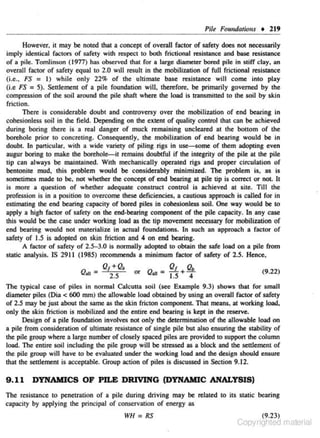
306. 282 • 111eory and PTClctice of Foundation Design
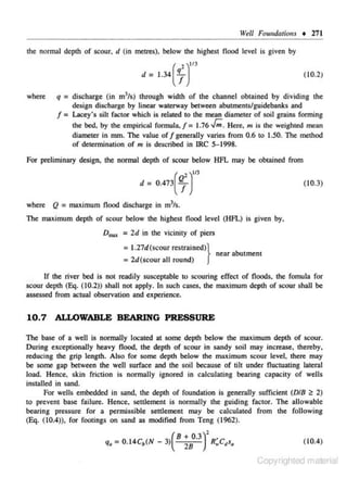
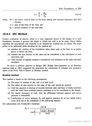
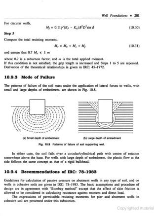
Case 1: Pier well (Fig. 10.9)
0
ic__rD_N ~
, .,
l
ul
Fig. 10.9 Active and passive pressure diagram for pier weJI in cohesive soil.
Depth or tension crack, d, =
where
D
= depth
2c[ii"; <: D
r
below scour line,
c = cohesion
r=
unit weight of soil
2
Permissible moment.
M, =
=
~ ( 2c.JN, ~
+ yDN,
~ ~) 8
~(~ rN,D'+ c.jN,D') s
( 10.32)
For d,<D
M=
,
(
~ [!rD'( N,- *)+cD2F.+ J~, )]s
(10.33)
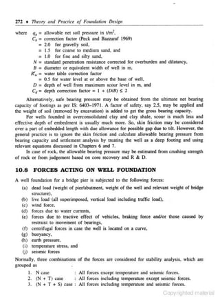
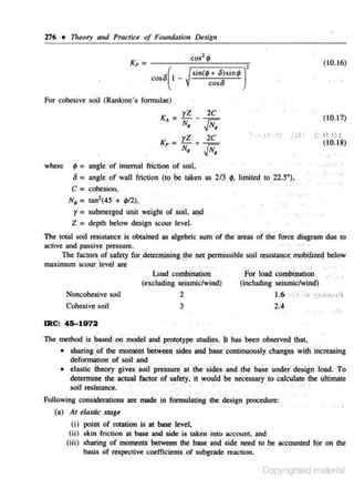
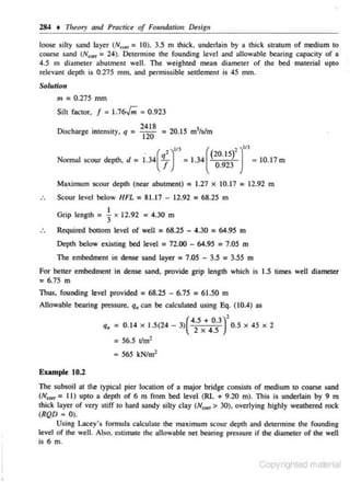
Case 2: Abutment well (Fig. 10.10)
Tension crack extends down ro a depth dr where net Pa = 0
D
1
(a)
(b)
(e)
Fig. 10.10 Active and pa$$1"' pre..ures on abutment well In 'e'L~Y."~~~Iiled
material

307. Well Foundations • 283
That is, (b) + (c) = (a)
or,
or,
( 10.34 )
For d, <:. D
then P. = 0, that is,
same as
in
case
I of pier well.
For d, < D. that is, (a) > (b) but < (b) + (c)
P• exists below dl"
At base,
M, = ![!rD'(N.- ;.) cH'(JN, ;;)]B- ~ B
2
+
+
Po
(10.35)
For (a) < (b)
Then net P. is trapezoidal.
At base,
(10.36)
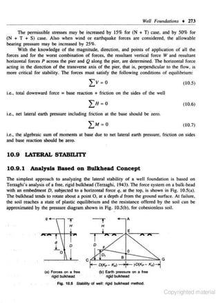
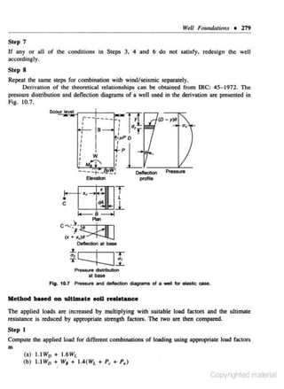
10. 10 WELL SINKING
The sinking or a well foundation is done by excavating the soil within the dredged hole. This
can be done manually or by mechanical dredger. A mechanical dredger consistS or prongs
with hard steel teeth which are pushed into the soil. When the dredger is pulled up, the
prongs c lose to form a bucket full of excavated soil. The mechanical dredger should be
adapced to suit the soil condition.
With increasing depth of well during well sinking, the friction on the sides of the well
increases. If the weight of the steining is not adequate to overcome the friction, suitable
kentledge may be placed on a platform 10 i!ICffiiSO the load on the steining. Air and water
jets are also used to minimize friction. Compressed air is used when well sinking is done
below water level to counter the water pressure inside the well.
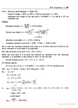
Example 10.1
A bridge 120 m long. is to be constructed over a river having Q..... = 2418 mlts,
HFL = 81.17 m; LWL = 73.00 m and existing bed level = 72.00 m. The subsoil consists of
Copyrighted material

308. 284 • TIJ~ory and Practict' of Foundation Design
loose silty sand layer (N.,... = 10). 3.5 m thick. underlain by a thick stmtum of medium to
coarse sand (NciJn = 24). .De1ermine the founding level and allowable bearing cap:LCity of a
4.5 m diameter nbutment well. The weighted mean diameter of the bed material upto
relevant depth is 0.275 mm. and pennissiblc settlement is 45 mm.
Solution
m = 0.275 mm
Silt factor.
f = 1.76..{,;; = 0.923
·
1sc
mtenslty. q =
D. harge ·
24 18
= 20.15 m 3/s/m
12 0
.
'
Nonnal scour depth. d = 1.34 ( ~ ) '" = 1.34 ((20. 15)' ) '" = 10.17 m
_
0 923
Ml>J<imum scour depth (near abutment) = 1.27 x 10.17 = 12.92 m
Scour level below HFL = 81.17 - 12.92 = 68.25 m
Grip length =
1
x 12.92 = 4.30 m
Required bottom level of well
= 68..25 -
4.30
=64.95 m
Depth below existing bed level = 72.00 - 64.95 = 7.05 m
The embedment in dense sand layer = 7.05 - 3.5 = 3.55 m
For better embedment in dense sand. provide grip length which is 1.5 times well diameter
= 6.75 m
Thus, founding level provided = 68.25 - 6.75 = 61.50 m
Allowable bearing pressure, q. can be calculated using Eq. (10.4) as
q. = 0.14
X
1.5(24- 3)(
2 x~s3 r 0.5 X 45 X 2
45
= 56.5 11m2
• 565 kNim2
Example 10.2
The subsoil at the typical pier location of a major bridge consists of q1edium to coarse sand
(N,., = I I) upto a depth of 6 m from bed level (RL + 9.20 m). This is underlain by 9 m
thick layer of very stiff to hard sandy silty clay (N""' > 30), overlying highly weathered rock
(RQD ~ 0).
Using Lacey·s formula calculate the mnximum scour depth and determine the founding
level of the well Also. estimate the allowable net beolring pressure if the diameter of the well
is 6 m.
Copyrighted material
•

309. Well Foundations • 285
Given: Maximum Oood discharge = 10.465 m 3/s
Lenglh of bridge = 382.5 m; HFL = 13.00 m; sill fac1or. f = 1.053;
submerged unil weigh! of soil and rock
wealhered rock.
= 10 kN/m 3; c' = 0; and f = 35• for
SoiMtion
Discharge intensity, q :: 10,465 - 27.36 ml /s/m.
.
382 5
NonnaJ scour deplh, d = 1.34 (
~
r
= 1.34(
(~~~s~T'
= 11.70 m
Maximum scour deplh = 2
x 11.70 = 23.40 m
Compu1 maximum scour level = 13.00 - 23.40 = - 10.40 m (RL)
ed
Bul as stiff clay overlying wealhered rock exists al 6 m below bed level (+9.20 m), lhe
above calculation of scour depth is not applicable.
Now take maximum scour level = 9.2 - 6.0 = 3.20 m
Below this level lhere is 9 m thick clay followed by wealhered rock. For reslricling
settlemen~ il is preferable 10 lake bollom of well 3 m inlo lhe rock.
Provide founding Level = 3.2 - (9 + 3) = - 8.8
m
For bearing capacily:
B = 6 m. D = 12 m. y' = 10 kN/m3• c' = 0, and f ' = 35• for wealhered rock
1
Now q,11 = y' D1 (N,- l)s,d• + O.Sy' BN1 s.,d1 w' + yD/
For
~
= 35°
N• = 32, N1 = 33,
'• = 1.2. s 1 = 0 .6
d• = d 1 =I+ 0.1
Or
q,11
:
(!}a+S
" I
(10 X 12 (32 - I)
+ (10 X 12)
X
3
+ { )"
1.2
X
I)
+ (0.5
X
10
X
6
X
33
X
0.6
X
J
X
0 .5)
= 4460 + 297 + 120
"' 4870 kN/m2
4870
3
" 1620 kN/m2
Copyrighted material

310. l86 • Theory and Pracn'ce of Foundation Design
As the well is founded on weatherM rock, settlement will be negligible.
Hence. allowable bearing pressun: = 1620 kN/ m2
Example 10.3
Using IRC methods, cheek the adequacy of design of the pier well of a bridge
(Fig. JO. II(a)). Use the following data on loads and soil propenies:
i7
FH
1
HFL 69.83 m
~ r;::::::::;:li_JJ<..:L"' l"" 68.16 m
W
H,
I !:1-~'- 3900--.il'--"800
800"""
10,822
-
Maximum acxu teve1
..........
.•..•..•.
.......... .....
..%,_.-l_h_or-1 ...... ..·.•
:ol; 57.638 m (2DJ
~:
~<.·
Sand
na:
Fig. 10.11(a) Plor well design fo< E-
10.3.
Loading:
Vet1ical Load:
DL = 12,400 kN
U
..
= 1390 kN
Total load = DL + U = 13,790 kN
Above well cap-8100 kN
Below well cap-5690 kN
Total
13,790 kN
Total horizontal fon:e, F H = 1755 kN
Moment at base = 43,180 kNm
Consider Tilt: I in 60
Shift
: 0.15 m
Soil Propern'es:
N,•• = 20; f = 33"; y = 19.2 kN/m3 ; li = 20"
Soil type: Coarse to medium sand
Consider permissible settlement of 1.5% of well diameter.
Copyrighted material

311. Hidden page

312. 288 • TIJUJ1)' and Prach'ce of Fou"dation Design
-----;;--~ -=;=~==;-r
c;:o;:s'
Kr =
cos.5(l _
si n(¢+ 8)sin; ) '
cos6
0.703
= 7.30
2
0.94 (1 - 0.68)
=
= 7.30 -
Kp - K•
0.265
= y'(Kp -
m
q=,
= 7.035
KA)cos8
= 9.2 X 7.035 X 0.94 = 61.8
3
I ( D' )
I
(12.678)
= 6m D + H = 6 x 6 1.8 x 12.678 + 11.925
= 839.3 kN/m2
Allowable horizontal fon:e,
Q
'"''
= q,...,B = 839·3 x 5 ·5 =2885 kN > 1755 kN (applied ron:e)
FS
1.6
He.nce, base pressure ([..,.) is only due to vertical fon:e.
f. . = w
"'"
A
s
13 790
•
= 564.6 kN/m2
24.42
Allowable bearing capacity. q.:
For
N = 20,
c.
= 1.5
Rw
= 0.5
8 = 5.5
c.,
=2
s. = 1.5% of 5500 = 82.5 mm
using &j. (10.4).
5
q. = 0. 14 x 1.5 x (20 _ 3>e:i
x~53 r o.5 ~ 2 x 82.5
= 81.9 • 800 kN/m2 > 564.6 kN/m2
Hence. this is accepltlble.
Method Based on IRC: 45 (elastic)
Step I
W
=13,790 kN,
M
= 48,680 kNm,
H
= 1755 kN
Copyrighted material

313. Well Foundations • 289
Step 2
D8 = 5500
18 =
I,
+ 2 x 38 = 5576 mm
~ (5.576)' =
= LIY
a
0.9
5.5 >< (12.678)3
J
= 840.574 m
12
X
12
p' = 13n
47.43 m4
o= tan 20" = 0.364
Jl = 13n ; = tan 33• = 0.649
B
5.5
a = lTD = 3.14 x 12.678 =
m = K,
K,
0 38
.I
= 1
I = 18 + ml, ( I + 2 f./a)
= 47.43 + I
X
840.574 ( I + 2
X
0.364
X
0.138)
= 972.45 m'
Step 3
r =
D(_l_) =
2
ml,
(12.678 )( 972.45 ) = 7 _
33
2
I x 840.574
M
48,680
-;:-(I + jJjJ' )- fiW =
_
( I + 0.649 X 0.364) - 0.649
7 33
8210 - 8950 -740 kN < H
=
,
-M( l-JJJJ) + pW =
r
=
X
13,790
X
13,790
=
48,680
_
(I - 0.649 X 0.364) + 0.649
7 33
5072.3 + 8950.7
14,023 kN > H
=
Step 4
mM
1
=
I x 48,680
_
972 45
=
so; r, (Kp- K.l = 9.2 x
with seismic. 1.25r'(Kp - K.)
Step
= 1.25 x
64.7
7.035 = 64.7
= 80.88' > 50
s
W - f./p±MB
A
21
: 13,790 - 0.364
24.42
= 465.8 ± 137.7
X
6641 :1: 48,680 X 5.5
2 X 972.45
= 603.5. 328.1 kN/m2 < 800 kN/m2• Hence, it is acceptable.
Method based on IRC: 45 (Uitilllllte)
Copyrighted material

314. Hidden page

315. Well Foundations • 291
Applied moment = 2439.6(24.603 - 0.2 x 12.678)
(Point of rotation 0.20 above base)
= 53.830 kNm < 68,500 kNm. Therefore. accepted.
Example 10.4
For the bridge considered in Example 10.3. check the adequacy of the abutment well whose
elevation and nature of earth pressure diagrams have been shown in Fig. 10.12
,.ll,
J:
f<- 4.500 m ...,
HFL 69.830m
-
Te
I
I
p,
N
~Max.
lfllUm SOOU'
d 62.088 (1.27d,)
E
&1
I .s
~
Foonding lew!
F
45
~60m
~
I
I • • Ill
•I
I•
>I
FlO. 10.12 Elevation and eanh pressure few bridge in Example 10.3.
Given:
Total Vertical Load V = 11,4n.8 kN
Horizontal Force F11 = 3446.5 kN
Moment M
= 17.020 kNm
Moment due to tilt and shift = 3840 kNm
Nonnal scour depth d, = 6.096 m
P. = 47.66 kNtm'
(refer Fig. 10.10)
Solution
•
Bombay method
M
11,020
t=H 1 +D=-=
= 22.35 m
·'F"
3446.5
D = 16.628 m
q,... =
v'
6
.
(H, + D)[y(Kp- K• )Dcoso- 3p.J
Copyrighted material

316. Hidden page

317. W~ll
Foundations + 293
IRC: 5-1998, Standard Specifications and Code at Practiu for Road Bridge, Section I,
General Features of Design, The Indian Roads Congress, New Delhi. 1998.
IRC: 45-1972.
Reco,urre~rdations
for Estimating tire ResistcUICe of Soil below tire Maximum
Scour L<v<l in the D«ign of Well Foundation ofBridg«, The Indian Roads Congress,
New Delhi, 1972.
IRC: 78-1983. Standard Specifications and Code of Practiu for Road Bridges, Section: VII,
Foundation and Substructure, 1st Revision, The Indian Roads Congress, New Delhi, 1994.
IS: 6403- 1971, Indian Standard Code of Practice for Determination of Allowable Bearing
PreSJure otr Shallow Found41ious, Indian Standard Institution, New Delhi, 1972.
Peck, R.B. and A.R.S.S. Bazuraf ( 1969), Discussion on Paper by D' Appolonia, el al.,
Journal Soil Mech. and Found. Div. ASCE, Vol. 95, SM. No. 3.
Teng, W.C. (1962), Foundation Design, Prentice Hall, Englewood Cliffs, New Jersey.
Terza8hi, K. (1943),
11~eoretical
Soil Mechanics, John Wiley and Sons, New York.
Copyrighted material

318. Foundations on
Expansive Soils
11.1 INTRODUCTION
Some cohesive soils undergo swelling when they come into contac. with water and shrink
t
when water is squeezed out. Foundations built on these soils undergo movement with
swelling and shrinkage of the soil. As a resul~ there is considerable cracking and other fonns
of distreos in the buildings.
Expansive soils are mostly found in the arid and semi-arid regions of the world. They
cover large areas of Africa, Australia, India, United States, South America, Myanmar and
some countries of Europe. In India, expansive soils cover nearly 2 percent of the land area
and are called black cotton soil because of their colour and conon growing potential. Large
areas of Dc<x:an plateau, Andhra Pradesh, Kamataka, Madhya Pradesh, and Maharastra have
deposits of expansive soil.
Expansive soiJs derive their swelling potential mainly from montmorillonite mineral
which is present in these soils. They are residual soils formed by the weathering of
basaltic rocks under alkaline environment. Extended periods of dry climate cause desiccation
of the soil but rains cause swelling near the ground surface. The depth of the swelling zone is
not much-being less than 5 m in most cases. However, lhe active zone over which lhere are
seasonal changes in moisture content. varies from l.S m to 4 m (O'NeiJI and Poormoayed,
1980).
11.2
•
NATURE OF EXPANSIVE SOU..
The swelling characteristics of a soil depend largely on the type of clay mineral present in the
soil. Differential Thermal Analysis (DTA), X-ray diffraction, and electrOn microscopy are
common methods of detennining the proportion of different minerals present in a soil. Some
simple laboratory tests are often used to determine the swelling potential of natural soil.
11.2 .1
Free-swell Test
This test is performed by pouring 10 g of dry soil, pa<Sing 425 micron sieve, in a 100 cc
gradunted cylinder filled with water. The soil collects at the bottom of the cylinder and
2114
Copyrighted material

319. Foundations on fxpoiiSive Soils + 295
gradually increases in volume. After 24 hours. the volume of the soil is read from the
graduations ip the cylioder. The pen:ent fru swell of the soil is given by
Free swell (%)
=
final
vo~u~e.: inilial volume x 100
·IOttlal volume
The pen:ent free swell of predominant clay minerals is given in Table 11.1. Kaolinite and
illite have percent free swell less than 100 and are generally regarded as non-swelling
minerals. MontmOrillonite, on the other hand, bas high sweiHng potential.
Table 11.1
Free swell of clay minerals
Ptrcent fne 1weU
Monunorillonite (Bentonite)
Kaolini1e
Utile
1201)...2000
80
»-'0
Gibbs and Holtz (1956) suggested that soils having fru swell above 50% may be expected to
cause problem to light sttuctures.
11.2 .2
Dtffenmtt.l Free Swell
Two samples of oven-dried soil (10 g) passing 425 micron sieve are taken and poured into
100 cc graduated glass cyliode~ne filled with water and the other with kerosene.
Kerosene, being a non-polar liquid does n(l( cause any volume change in the soil. After 24
hour$, the volumes of soil in the two cylinder$ are measured aod the differential free swell.
DFS is obWned
DFS
~ soil volume in water- soH volume in kerosene x JOO
soil volume in kerosene
IS 2720 (Part lll-1980) gives the degree expansiveness of a soil in terms of the
differential fru swell, Table 11.2.
Table U .l Oregrce or ex.paosJveness and DFS
DFS ('J>}
Low
Moderate
High
Very high
Lc:ss than 20
20-35
35-50
Ot<Okt than
so
11.2.3 Unrestrained Swell Test
This test is done in the standard odometer. The soil specimen is given a small surcharge load
(say. 5 kN/m2) and submerged in water. The volume expansion of the specimen is measured
in terms of the increase in thickness of the specimen-the cross·sec tiona~ area remaining
consranr. The percent swell is expressed as
Copyrighted material

320. 296 • Tlteory and Practice of FoundaJiorr Desig11
s.(%)
=
!J.H
H
x 100
where, s.(%) = free swell,
6.H = increase in height of soil sample. and
H = original height.
Vijayvergiya and Ghazzali (1973) gave a correlation between free swell. natural moisture
contenl. and liquid limit of some clays. This correlation is presented in Fig. 11 .1.
20
to
1'
1
l.:"{ • 70
1~0~
1
J
'
0.1
0
10
20
30
40
50
Natu"" - · content (%)
f'G. 11.1 ReladooJhlp between hee swen., water content. and
(aftO< Vijaywrglya and Gha:Wii, 1973).
11.2 .4
l~ukl
limit
Swe>Ding Prenure
The swelling pressure indicates the external presswe required to prevent swelling of a soil
when the latter comes into contact with water. The test is done in the consolidation
apparatus. Water is added to the specimen and as it stans to swell. pressure is applied in
small incremeniS to prevent swelling. The test is continued till lhe sample just begins to
settle. This gives the swelling pressure (p,) of lhe sample (Sridharan et al. 1986). As a
general rule, a swelling pressure of 2()...30 kN/m2 is considered low. A highly swelling soil,
for example, bentonite may have swelling pressure as high as 1501)...2000 kN/m 2•
Some empirical formulae have been suggested for estimating the swelling pressure of a
soil from lhe void ratio and plasticity
p,
ind~x
=
of the soil (Pidgeon. 1987).
2 - 24(;/)
.7
Copyrighted material

321. Foundations on Expansive Soils • 297
where, p, = swelling pressure (kglcm2),
ei :: initial void ratio, and
PI = plasticity inde< (%).
11.2 .5
Clasaiflcation of Swe111ng Potential
Potential sweiJ is defined as the vertic.al sweiJ under a pressure equal to overburden pressure.
A number of cla.~ification systems for the swelling potential have been proposed (Seed et at.
1962: Sowers and Sowers, 1970: Chen, 1988; Vijayvergiya and Ghazzali 1973). These are
generally based on the Atterberg Umits of the soil. O' Neill and Poormoayed ( 1980)
summ.:irized the U.S. Army Waterways Experiment Station criterion based on plasticity index
and the potential swell. This classification of expansive soil is expressed in Table 11 .3.
Tab&t 11.3 Classification or e.xpansive soil
Uquid limit
Pot~nJial modi
Plas.ticity inda
S~vlling pot~ntitJI
<SO
<25
< 0.5
Low
~(,()
25-lS
> 3S
O.S-I .S
> I.S
Marginal
>00
Higl>
USBR (1960) gives similar criteria for clays based on colloid percent Oess than 0.001 mm)
and shrinkage limit of the soil, which arc shown in Table 11.4.
Table 11.4 Criteria for expansh·e clays
Colloid
Plasticity lnda
Shrin!a1~
limit
C()ttlmf ('~!)
> 28
2~30
13--23
< iS
> 3S
2S-41
IS-28
> 10
<II
7- 12
IQ-16
> IS
Proboblr
uponsion (~)
> 30
2Q-30
IQ-20
< 10
Dtgru of
uponsit.·M.eu
Very high
Hiah
Medium
Low
U .S EFFECT OF SWELLING ON BUILDING FOUNDATIONS
In tropical countries, the soil near the ground surface dries up during the summer as a
consequence of intense heat and recession of ground water table. The soil becomes stiff and
cracks and fissures open up. When rains come. the soil gelS wet by the precipitation and with
time, the ground water table also rises. This causes increase in water content of the soil and
hence, swelling of the soil. The structure built on the soil protects the soil from the heat but
nonetheless water tends to accumulate from the surrounding areas and contributes to swelling.
The depth over which such variation in water content occurs depends on the nature of soil
and cliii'Uitic conditions but an active zone of 35-4 m has generally been observed.
The movement of the foundation with swelling and shrinkage of the soil causes the
floor slabs of buildings to lift up and develop a dome shaped deformation pattern. This leads
to cracks in the floor and external walls. The diffen:ntjal movement also cause$ diagonal
Copyrighted material

322. 298 • Theory and Prac tice of Foundati011 Design
cracks in the walls and at the corner of doors and windows. as shown in Fig. ll.2 Utilities
buried in the soil get damaged and the leakage of water into the soil results in funher
swelling. The effect is more pronounced in the one or two storey buildings where the
foundation pressure is often Jess than the swelling pressure. For Ulll structu res, foundation
pressure generally exceeds rhe sw~ll::tg press ure and the swelling potential reduces.
Roof sl&b
FlOOr stab
heaved
t t t
Expansion
Fi g. 11.2 Oi$tress In buildings due
to swelling.
11.4 FOUNDATION DESIGN IN EXPANSIVE SOD..
Foundation design in expansive soil needs a different approach as compared to that in
non-swelling soil. II must be realized that limiting the snfe bearing pressure to a low value
does not help to counteract the swelling pressure. Rather. design should be done with a high
enough bearing pressure and following the criteria of beaiing capacity failure and pennissible
of settlement. so that chances of swelling are minimized.
Foundation design in expansive soil c:an be done in the following ways:
l. lsol:uing the foundation from the swelling soil,
2. Taking measures to prevent the swelling. and
3. Employing measures to make the structure withstand the movement.
11.4.1
Isolating the Foundation from the Swelling Zone:
Under-reamed Piles
A common method of building fou ndation in expansive soil is to provide under-reamed piles
below the foundation. Here. the structural load is transferred to the soil beneath the zone of
Outtuation of water content. The piles are taken to depths of 5- 6 m, that is. well beyond the
expansive zone. These piles are bored cast-in-situ piles with the lower end e nlarged to fonn
under-reamed bulbs with the help of special tools. Fig. 11 .3. The piles generally have shaft
Copyrighted material

323. Fouudotlmu on Expo11J·ive Soils • 299
diameter of 300 mm and bulb diameter of 750 mm. as depicted in Fig. 11.4. The piles are
fixed at the top to RCC plinth beams. A gap of 75- 100 mm is kep~ between the-plinth beam
and the soil which is filled with granular material 10 pe- nit swelling of the undetlying soil
n
without straining the plinth beam-s. The piles are adequately reinforced 10 take care of the
uplift forces caused by the swelling ac1ion of the soil.
Kelly
caslng
(3)
aouom hinge
Flg. 11.3 TOOls
(b) T01> hinge
tor bulb fotmatlon
in under-teamed
d
~=Mles.
(anor Tomlinson. 1994)
d
!L
A
'AT
:
/<t."-.
"
Sin~
1..,
'A.l_
/
under-ream
Double under·ream
Flg. 11... Typical under·re.amed pile found.ation.
Copyrighted material

324. 300 • 11reory a11d Practice of Foundation Desigu
The ultimate being capacity of an under· reamcd pile is determined from static analysis
as already discussed in Chapter 9.
Q. = aC,1 11 + c.,Ar. + A,N,C,, + A.,N, Cpz
A
where.
A11
At'1
(1 1.1)'
= surface area of pile stem,
= surface area
of cylinder circumscribing the under-reamed bulbs.
Cu 1 = undrained shear strength of soil around pile s haft.
c.2 = undrained shear strength of soil around under-reamed bulbs.
Cp 1
= undrained shear strength
below pile tip,
Cp: = undrained shear strength below under-reamed bulbs.
a = adhesion factor along pile stem,
A P = cross-sectional area of pile toe.
= bearing capacity faclor. usually taken as 9.0. and
A. = (tr/4)(D;- D"J where D. and Dare the bulb and stem diameters respectively.
N•.
The safe capacity of the pile may be obtained by applying a factor of safety of 2S-3. The
uplift capacity of under-reamed piles are obtained from Eq. (11.1) but without considering
the end bearing component A,N,Cpl·
The main fun clion of under-renmed piles is to transmit the vertical Joad into the soil
below the swelling zone. ln case the soil above the under-reamed section tends to s well, uplift
forces are creared on the foundation which the under-reamed bulbs would be able 10 counrer.
There is some doubl over 1he practicability of forming the under-reamed bulbs in granular soil.
Obviously. the under-reamed section of the pile should be able to stJ>nd on its inclined faces
during boring and till the concreting is done. For this. sufficient cohesion should be available.
Clayey soil provides this cohesion without much difficuhy. But the fonnation of bulb i n
granular soil is not free from uncertainties. Field experiments have shown that the sand tends to
disintegmte during the stand up time and no bulb is really formed.
It should also be noted that the under-reamed piles should penetrate well into the firm
gromld to give sufficient end bearing at lhe level of the under-retlms. Presence of soft clay
benenth the expansive soil would preclude the use of under-reamed piles. Indiscriminate use
of under-reamed piles simply because the soil at ground surface is expansive in narure., ofren
serves no useful purpose.
11.4.2 Controlling Swelling
Impervioua apron
Swelling of soil near the ground surface can be controlled by providing an impervious apron
around the s tructure as illustrated in Fig. L1.5. This prevents surfac-e precipilation from
penetrating inro the soil but the sea..o;onal rise of ground water .table is not controlled. The
impervious apron is generally made of bituminous concrere but it should be sufficiently
flexible to prevent c racking and distress due to soil movement caused by swelling. It is
necessary fo r the apron to penetrate sufficiently into the foundation to prevent ingress of
water into the soil during inundation.
Copyrighted material

325. Foundations on E.rpans;ve Soils • 301
Brick waJI
AI
sa<* fiU
Fig. 11.5 lmpeMous apron for oontrollino swelling,
Swelling can also be controlled by applying a pressure on the ground at least equal to the
swelling pressure of the soil. Attempts have been made to apply a surcharge on the footing
but this does not prevent the swelling between foundations. l.f surcharge loading is to be
applied, this should be done to cover the entire building area by a suitable non-swelling soil.
The depth of surcharge should, or course, be such that the surcharge pressure is at least equal
to the swelling pressure of the soil. Surcharge loading is depicted in Fig. 11.6.
area
Surcharge pressure
rD • p,
D
t
t
l
Swelling pressure p,
FliJ. 11.1 Surd'large k:llding k> control Swelling.
CNS layer
Katti (1979) proposed the use of a cOheaivenon·swelling (CNS) layer to reduce the effect of
swelling. A clay soil of adequate thickness having non-swelling clay minerals, is placed on
the subgradc and the foundations arc placed on this layer. The optimum thickness of the CNS
layer is to be detennined from large scale tests. The method has been used in canal lining
works, as shown in Fig.. 11.7 but its use in foundations is still limiled.
Ac:tlWt zone
Fig. 11.7 Use of CNS layer In canal llninQ.
Copyrighted material

326. 302 • The0')1 and Practice of Foundation Design
Chemical Stabilization
Attempts have been made to control the swelling potential of expansive soil by lime-slurry or
limc·flynsh injection. Such injection is done through pressure grouting technique on a close
grid around the foundation to cover the entire foundation on:n. Bu1 the method is expensive
and has not been widely used. However, lime slurry injection has been used to stabilize
foundations on expansive soil after occurrence of distress.
11.4.3
Measures to Withstand Settlement
Tile foundation may be made sufficienlly rigid by providing interconnected beams and band
lintel to withstand the effects of differential movement on the structure. Stiffened mat
foundations (Lytton. 1972) have also been adopted to counter the effect of diffe.rential
ground movement. Premlatha (2002) carried out a study on the use of stiffened mat for low
rise structures in Chennai, based on evaluation of heave of the soil. A three dimensional soil
structure interactive analysis was done 10 suit the loading. climate. and environmental
c.onditions of Chennai. However. these methods are rather expensive and have not been
widely used for low to medium structures.
Design of building fou ndation in expansive soil needs careful evaluation of the swelling
potential of the soil in terms of the mineralogy. Attcrbcrg Limits. and the swelling pressure.
Mineralogy and Atterberg limits indicate the ne(.-essity or otherwise of special design. Only
swelling pressure gives a true understanding of the magnitude of the swelling potential. In
particular. light structures are more vulnerable to distress because the bearing pressure is
often less than the swelling pressure and the foundation is prone 10 uplift forces. For a
minimum depth of foundation of 2 m with the bottom of the trench filled with sand, a
broken stone is ofren used to minimize the effect of swelling RCC plinth beams. Band lintel
also helps 10 withstand the effect or swelling.
Under-reamed piles and s urcharge loading seem to be the most suitable methods of
countering the effect of s welling. In addition, good surface drainage and impervious paving
around the s ite help 10 prevent wa1er percolation in the soil.
Chen. F.H. ( 1988). Foundations on Expansive Soils. Elsevier. Ams·tcrdam.
Gibbs. H.J. and V.G. Holtz (1956), £ugl11eeri"g PropuHt!s of Expa11sive Clays. Transactions
ASCE, New York. Vol. 121, pp. 641-663. Paper No. 28 14, Discussion. pp. 664-777.
IS 2720 (Port lll-1980), M•llsureme~lr of Swelling Prusure of Soil.<. Bureau or Indian
Standards. New Delhi.
Koui. R. K. (1979). Search for Solutions to Problem.< in Block Conon Soils, First IGS
Annual Lecture, Indian Geoteclmical Joumal, No. t , Vot 9.
Lyuon, R.L. ( 1972). Desigu Method for Coucrete Mllts 011 U11stab/e Soils. Proceedings 3rd
American Conference on Materials Tech .. Rio-de-Janeiro, Brazil. pp. 171 - 177.
Copyrighted material

327. Foundations
011
Expansiv~
Soils
+ 303
O'Neill. M.W. a nd N. Poormoayed. ( 1980), Methodology for Foundations on Expansive
Clays. Joumal of the Geotechnical Engineering Division. American Society of Civil
Engi ncc~ . Vol. 106. No. GTI2, pp. 1345-1367.
Pidgeon. J.T. (1987), A Compariso11 of E.tisti11g Methods for the Desig11 of Stif!
e11ed R'a/r
Foundation on Expansion Soil. Proceeding 7th Regional Conference of Africa on
SMFE. pp. 277-289.
Premla1ha. K.. (2002). Predicliou of HuJve U.siug SoU- Water C!JaracteriJtics and Ana/y.sb of
Stiffened Raft 011 Expansive Clay.s of Chennm·. Ph. D. Thesis, Anna University. Chcnnai.
Seed, H.B., R.J. Woodward. Jr.. and R. Lundgren ( 1962). Prediction of Swelling Potential
for Compacted Clays, Joumal of the Soil Mechanics 011d Foundations Divlslon.
American Society of Civil Engineers, Vol. 88, No. SM3, pp. 53-87.
Sowets. G.B. and G.F. Sowers (1970). Introductory Soil Meclwnics and FoutJdations, 3rd
ed., New York. Macmillan.
USBR (1960), &mit MaJ111al. U.S. Bureau of Reclamation, Denver, Colorado. July. 1960.
Vijayvergiya V.N. and 0.1. Gha.uali ( 1973). Prediction of Swelling Potemial of Nawral
Clays. Proceedings 3rd lnrernar
ional Research and Engineering Conference on
Expansive Clays. pp. 227- 234.
Copyrighted material

328. Ground Improvement
Techniques
12.1 INTRODUCTION
Soils are deposited or fanned by nature under different environmental conditions. Man does
not have any control on the process of soil formation. As such the soil str:lla at a site arc co
be accepted as they are and any construction has to be adap!ed to suit the subsoil condition.
The existing soil at a given site may not be suitable for supporting lhe des~ facilities such
as buildings, bridges. dams. and so on because safe bearing capacity of a soil may not be
adequate to suppon the given load. Although pile foundations =y be adopted in some
situations, they often become too expensive for low to medium·rise buildings. In such cases~
the properties of the soil within lhe zone of influence have to be improved in order to make
them suitable to suppon the given load.
Ground improvement for the purpose of foundation construction essentially means
increasing the shear strength of the soil and reducing the compressibility to a desired extent.
A number of ground improvement techniques have been developed in the last fifty years.
Some of these techniques need specialized equipment to achieve the desired resuJt. In this
chapter. only the common ground improvement techniques tthich use simple mechanical
means to improve soil properties for low to mec:Uum·rise strucrures are considered. For tall
structures. pile foundatio ns with or without basement would generally give the most
economic foundations.
12.2
PRINCIPLES OF GROUND IMPROVEMENT
The mechanics of ground improvement depends largely on the type of soil-its grain-size
distribution, water content. structural arrangement of particles and so forth. lo general,
ground improvement is caJied for in soft cohesive soil with low undrained shear strength
(c. < 2.5 t/m2 ) and loose sand (N < 10 blows per 30 em). The mechanics of ground
improvement can be understood in terms of the structural arrangement of particles
constituting the soil deposit.
(a) Cohesive ooU
Sedimentary (alluvial or marine) clays during deposition under nowing water have the
flexible flake shaped panicles arranged at random flocculated Sltucture with large void spaces
S04
Copyrighted material

329. Grou11d
lmprol!em~nt
Tecll11iques + 305
filled with water. Figure 12.1(a) depicts the flocculated structure of cohesive soil. Such
structural arTangement with high water content is unstable and gives high compressibility.
Under the influence of increasing overburden pressure or extemaJ load. the soil consolidates
and the particles tend to re-orient themselves along horizontal planes (that is, perpendicular to
the line of action of the applied load). Such a dispersed structure is more stable and the
reduction of water content brings the particles closer tOgether to reduce compressibiJity. as
shown in Fig. 12.1(b). Thus, reduction of water content through application of external load
would cause improvement of engineering properties of cohesive soil.
_ 7 ___ ---....- -- - '
, --....._-
--.---
--~r~~
-----~ ---- ~ -------_ ..,__ -,- __l_ __ "-~
~
-=~-=s~~~~~
-
----~--------~~~
-----.
- -------.----------------------------------------
~=-:---=-~ --=---:
-=='J"
---------------------
(a) Flocculated strucblr&.
(b) Oiopo<Hd &11Jdln.
Flg. 12.1 Slruclunl olcoheolve ool.
Cohesive soil can be fmproved using
(a) Preloading with .venical drains and
(b) Soil reinforcement with stone columns.
(b)
Granular ooll
Panicles of granular soil such as sand and gravel, have three-dimensional structure. For the
purpose of understanding, they can be represented by spheres which in loose condition are
arranged one on top of the other as shown in Fig. 12.2(a). Granular soils in this condition
have low relative density. The shear strength is also low because of the tendency of the
panicles to roll over one anothu under the influence of shearing stresses. lf the same
panicles are rearranged as shown in Fig. 12.2(b), the void space decreases and the relative
(a) Loose structure.
(b) Dense stnJclure.
Fig. 12.2 Structure of granular soil.
Copyrighted material

330. 306 • Theory and Practice of Foundation Design
density increases with corresponding increase of shear strcQ&dl. Thus, properties of granular
soil can be improved by increasing its relative density by external means. Following ground
improvement techniques are used for granular soil:
(a) Compaction wilh drop hammer and
(b)" Deep compaction by compaction piles or vibrofloatation.
Apan from these, soil reinforcement by inserting stiffer materials within the soil fabric
such as metallic strips, compacted granular piles, geotextiles, and so on would also improve
the propenies of the soil which then behave as reinforced mass. Figure 12.3 depicts soil
reinforcement technique.
Flg. 12.3 Soil relnforolmenl
Chemical injection and grouting are also adopted as methods of ground improvemcnL
In these cases, the chemicals penetrate into the voids and get set to strengthen the soil fabric.
Normally, these techniques require specialized equipment to achieve success in the field.
These methods are not discussed in this chapter.
12.3 GROU1'1D TREATMENT IN COHESIVE SOIL
12.3.1 Prelo•dlng with Vertical Dra1u
The most cornrno o method of ground treatment in cohesive soil is to reduce the void ratio or
water content of the soil by preconsolidation. This increases the shear strengrh of the soil and
re<uces the compressibility even before construction of the building is commenced.
Figure 12.4 displays preloading for building foundations. Soil propenies are improved under
the preload to the extent required to support the building.
SOft day
--------- - • ..........
Re"""" pr- and
oon.struct building
Fig. 12.4
Preloadlng f« buldlng founclallons.
Copyrighted material

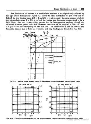
332. 308 +
111~ory
and Practice of Foundation Design
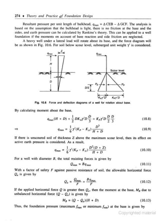
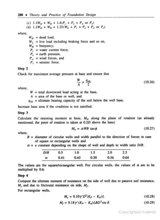
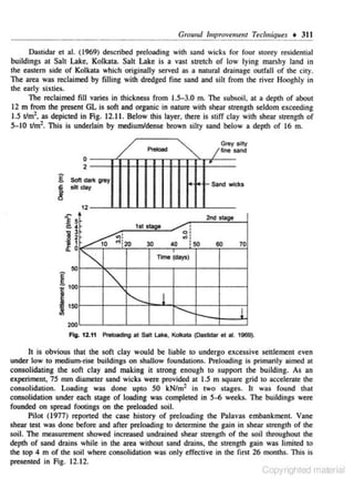
In the earlier days, sand drains, 300-500 mm diamerer, were insralled by filling with
sand the vertical holes made into the soil at predetermined spacing. Nowadays sand wicks and
prefabricned venical drains (PVD), e.g., band drains are mostly used ro have more efficienr
consolidarion under the preload. When a soil is preloaded by dead weighr, the horizonral
drainage path is reduced and the soil undergoes radial drainage. Each drain well has an
axisymmetric Zone of influence with a radius approximately l/2 times the well spacing. 1be
flow "!ithin the zone is a combination of radjaJ flow towards lhe sand drain and vertical flow
towards the free-draining boundary. The average degree of consolidation is rhen given by,
U=
where
I - (I - U•)(l -
UiJ
(12. 1)
u.
= average degree of consolidation due to radial drainage and
Uz = average degree of consolidation due to vertical drainage.
Assuming unifonn vertical strain ar the surface, Barron (1948) gave the expression for degree
of consolidation due to radial drainage as,
u. =
2
where F.= (
n
"
2
n -I
)log.n -
I - exp(-
T, =
c,:
d,
dra1 n d tameter
. '
= radial
(12.2)
(3n'~ 1).
4n
= !!.J_ _ equivalent drain spacing
d ,.. -
s;:)
d
• an
time factOr.
The drains may be insralled in either square or triangular grid. Considering the influence area
of each drain to be circular. we have
d~ = 1.13s for square pattern
}
(12.3)
• LOSs for triangular pattern
where
s = actual drain spacing (refer Fig. 12.7).
SQuare grid Triangular grid
s
ct. •1.13s
n • d.Jd.,
Fig, 12.1
s
ct. • t.05s
T, =c,tld]
Spadng of vertical drains.
Copyrighted material

333. Hidden page

334. 310 • Theory and Practice of Foundation Design
covered with a drainage blanket. The sand wicks may be of 55- 75 mm diameter and can be
installed at spacing of 1- 2 m.
(c) Band drains: Band drains or fabric drains are usually 7S-100 mm wide and 3-5 mm
thick made of synthetic fabric with high permeability. They are installed in the ground by
special mandrel and cranes.
In addition to the above cardboard drains (KjeUman, 1948) and rope drains have also
been used. Different types o.f vertical drains are shown in Fig. 12.9.
fabric
Band dralno
Field control is essential for any preloading work. It is necessary to ensure that the
consolidation under preload is essenliaUy complete before the building is builL Settlement
and pore-pressure measurement give useful information in this regard. A simple
insuumenration scheme is shown in Fig. 12.10. In most routine jobs, settlement measurement
on vertical rods and pore-pressure measurement with a few standpipe piezometers, around the
periphery of the preload should be sufficient.
Fif!J. 12.10 Preloecing: field measurement scheme.
Copyrighted material

335. Gr01md Improvement Teclmiqu~s + 311
Dastidar et al. (1969) described preloading with sand wicks for four storey residential
buildings at Salt Lake, Kolkata. Salt Lake is a vast stretch of low lying marshy land in
the eastern side of Kolkata which originally served as a natural drainage outfall of the city.
The area was reclaimed by filling with dredged fine sand and silt from the river Hooghly in
the early sixties.
The reclaimed fill varies in thickness from 1.5-3.0 m. The subsoil. at a depth of about
12 m from the present GL is soft and organic in nature with shear strength seldom exceeding
1.5 tlm2, as depicted in Fig. 12.11. Below this layer, there is stiff clay with shear strength of
5-10 tlm2. This is underlain by medium/dense brown silty sand below a depth of 16 m.
- ""'
0
2
E
g
SOft dark gray
sill day
/Grey Silty
flne
sand
Sand wicks
12
2nd stage
5
i.~:20
.,:
0
I~
tst
'
stage
30
•
..
"''
•
O•
40
:so
60
70
Time tdays)
""
['......
l ........_
l
200
Fig. 12.11 Preload~ at San Lake, KOikata (Oastidar et al. 1969).
II is obvious that the soft clay wou.ld be liable to undergo excessive settlement even
under low to medium-rise buildings on shallow foundations. Prelooding is primarily aimed 111
consolidating the sof1 c lay and making it strong e nough to suppon the building. As an
experiment, 75 m.m diameter sand wicks were provided at l.S m square grid to accelerate the
consolidation. Loading was done upto SO kN/m2 in two stages. It was found that
consolidation under each stage of loading was completed in 5-6 weeks. The buildings were
founded on spread footings on the preloaded soil.
Pilot (1977) reponed the case history of preloading the Palavas embankment. Vane
shear test was done before and after preloading to determine the gain in shear strength or the
soil. The measurement showed increased undrained shear strength of the soil throughoot the
depth of sand dro.ins while in the area without sand dro.ins. the strength gain was limited to
the top 4 m of ahe soil where consolidation was only effective in the first 26 months. This is
presented in Fig. 12. 12.
Copyrighted material

336. Hidden page

337. Hidden page

338. 3 14 • Theory and Practice of Found4tioo
~sigo
Preloading for a single building with little wori<ing space in the surrounding may 1101
be always feasible from considetltions of time and cost. Although theoretically sound, the
C0$1 of preloading per unit area goes up on accounl of the high cost of uansportalioo ·
""JUited 10 mobilize the preload and then 10 dispMe of the preload. Typically, a single sllge
preloading job needs a time of al least 10-12 weeks before a site may be made ready for
con&trUCiioo. The following srages of work are involved in the process:
(a) insullalion of saod wicks,
(b) laying drainage blanke~
(c) mobilizing the preload,
(d) lime for consolidation, and
(e) removal of preload.
Preloadiog is bes< suiled when a l~~~&e numbet of medium-rise buildings are ""Julted to
be buill in a consuuction project. M ultiple use of the sand wiclting equipment and the
preload material reduce the unit coot.
12.3 .2 Stone Columne .
A suitable technique of ground improvement for foundations on soft clay is to iosull vertical
stone columns in the ground. Stone columns are essentially a method of soil reinforcement in
which soft cohesive soil is reploced at discrete points by compacted stone or crushed rock in
pre-bored vertical holes to form 'columns' or 'piles' within the soil. The stooe columns serve
two basic functions, namely
(a) providing suength relnfon:ement to the soil and
(b) acting as vertical drains 10 allow subsoil consolidation to occur quickly under any
given loading.
Greater stiffness of stone colunms compared 10 that of the •urrounding soil cauaes a
large portion of the vertical load to be transferred to the columns. The entire soil below a
foundation, therefore, acts as a reinforced soil with higher load carrying capacity than the
virgin ground. FUrther, pori-pressure dissipation by radial Oow accelerates the consolidalion
of the subsoil. Engelhardt et al. (1974) dernonstraled the beneficial effects of stone coiWilDS
by canying out load tests in soft claY with and without stone column reinforcement.
F~gure 12.14 is a graphical representation of the same.
0
-(kPI)
1!!0
200
2SO
-20
i
J:
Wllhoulcdumn
llll
Fig. 12. 14 Elledlvenns ol slono cclt.mns (Enge4h- e1 el.. 1974).
-.
Copyrighted material

339. Ground lmpro-.-nt Tecluoiqws • 315
eo...tnactJoG technique
Installation of stone columns in soft clay may be done in two ways:
(a) Vibratory technique using vibroROI and
(b) Rammed stone column technique.
1be basic tool used in these techniques is a poker vibrator or
vibroflo~
as shown in
Fig. 12.15, which is 2.0-3.0 ·m long with a diameter varying between 300 mm to 300 mm.
Extension tubes are attached to the vibrofiOI whenever greater depth of uutment is needed.
1be vibrofiot is a hollow steel tube containing an eccentric weight mounted at me bottom of a
vertical shaft; the energy is imparted by routional mocion through the shaft while the eccentric
wejghl impans vibration in a horizontal plane. Vibration frequencies are fixed at 30 lh or
t. Botlr1g .... -
2. Ccrrc>ac:tlon
3.-
'".l;r;:= Ultillg poJiey
tMooofold Wallt hoMs
H)'draiAic llooea
f---F--.a
Ftg. 12.15 Stone co1urm instalillion by liblolollllon.
Copyrighted material

340. 3 16 • Theory and Practice of Foundmion Desig11
SO Hz to suit electric power cycles. The free fall amplitude varies between S- 10 mm. The
machine is suspended from a vibration damping connector by follower tubes through which
power lines and water pipes pass. These allow simultaneous release of water jets to remove the
soil around the vibroflot as the latter makes its way into the hole under venical pressure from
the top. When the vibroflot reaches the desired depth, tbe water jet at the lower end is cut off
and granular backfill is poured through the annular space between the ~ole and the vertical pipe
by head load or conveyor as the vibnuory poker is withdrawn. Well graded stone backfill of
size 1S mm to 2 mm is used and compaction is achieved by vibration of the poker as it is Hfted
up: Due to compaction, the stones are pushed sideways into the soft soil to produce a stone
column of diameter larger than the diameter of the borehole. Normally, 600-900 mm diameter.
stone column can be obtai~d for 300-SOO mm diameter vibroflot.
R•••ed Hone coliiiDD
This installation technique was proposed by Datye and Nagaraju (1977) and developed fuither
by Nayak (1983). In this technique. the granular fill is introduced into a pre-bored hole and
compacted by operating a heavy rammer through the borehole. The hole is made by using
normal bored piling rig with winch, bailer. and casing. The method of installation is illustrated
in Fig. 12.16. To facilitate charging of the granular aggregate into the borehole, windows with
hinged flap valves opening outSide are provided to the casing at interval of
2 m or so. These windows are kept: in cloSed position during driving or withdrawal of casing by
screwing nuts 10 prevent ingress of soil into the granular backfill. For installing stOne columns
10 greater depths, more than one piece of casing is used with the help of special quick release
c<>uplings. The casing majntains the stability of borehole. The stone columns are required 10
function as drain weUs and il is advised not to usc bentonilc slurry for maintaining the stability
of the borehole. Backfill material should be such that it gives high angle of internal friction
•
Ht..:>ll-- Bailer
wen graded baclrnll ..
75mmto2mm
0
..
Fig. 12.16 Stone ¢01vmn lnstallalion by ramming methOd.
Copyrighted material
"

341. Ground Improvement Techniques • 317
under given energy of compaction. Sometimes the mixtures of stone aggregate and sand,.
generally in proponion of 2:1, are used as ba.:kfill material. It is observed that sand is utilized
mainly in filling the voids in gravel skeleton. Gravel backfill of aggregate size 7S mm to 2 mm
is generally rccommonded. The gravel should be well graded and preferably angular shaped for
good interlock. The main purpose of compaction is to rearrange the stone particles so that very
good interlocking between panicles is obtail:'led to give high angle of intemal friction. Too
muc.h ram.ming, however, crushes the aggregate. For a given compaction energy, greater weight
and smaller drop of the rammer give better results.
Comparison of cODStnlctiOD teclml.qaea
All the inslllllation techniques for stone columns in soft clay are self-adjusting in tlie sense that
enlargement of the column during ramming or vibration occurs depending on the soil
consistency. figure 12.17 shows the range of soil suitable for such a treatment by stone
columns.
4
10
20
Fig. 12.17 Range
o(
40 60
d
140 20Q
suitable f<>r -~ by..,. columns.
Rammed stone columns have been used extensively in lndia. They are found to be quite
suitable for all k.i nds of soil (Datye 1982). Nayak (1982) has suggested that the angle of
internal friction, ;· may be as high as 45° for compacted granular fi ll in rammed stone
column. whereas for vibrofl.oted stone column 4/ ranges between 38°-42°. It is also to be
noted that in vibrofloted s tone column, the top about I m deep does not get properly
compacted for lack of ~nflnement near the surface, whereas in practice this portion of the
s tone column is required to take greater Joad intensity. ln case of rammed stone column,
proper compaction can be achieved even for this length because of lateral confinement of the
Copyrighted material

342. 318 • 17teory and Practice of FoundDtion Design
casing pipe. Willi vibrollot, lbere is no harm in using high energy of compaction. Ralhc:r, it
reoulu in larger diameter of the stone column and better compaction of aggregate to give
higher value of angle of internal friction. Net effect of this is to increase the loed carrying
capacity of the stone column. But for rammed stone column, such high compaction energy
may crush the aggregates, resulting in lower value of ;• and lower capacity of the stone
columns. In general, however, vibroflotation needs skilled labour and better quality control
while the installation of rammed stone columns needs greater manpower. (hoerall, rammed
stone column appears to be more economical although it is a very slow process compared to
vibroflotation.
Dnlp pdaclplea
The deaign of stone column fOIIIIdMion involves the .......,.,nt of
(i) diameter of stone column.
(ii) depth of stone colwm, and
(iii) spacing of stone column.
D-.-,er of 110M colamn: For a particular driving method, vibroDotation oc rammed stone
column, the diamecer of the finished stone column depends on the strength and consistency of
the soil, the energy of compaction In rammed column, and diameter of poker with fins of the
vibrollot. The softer the soil, greater is the diameter of the pile because compaction of the
aggregate pushes the stone into the surrounding soil. The diameter of pile installed by
vibroOot varies from 0.6 m in stiff clay to 1.1 m in very soft clay. Rao and Ranjan (1985)
reported that using the rammed ~e<hnique, the installed pile diasneter is about 20-25% more
. than the initial diameter of the borehole. Nayak (1982) has given a chart to correlate the
diameter of stone column and the undrained shear strength of soil, as depidod in Fig. 12.18.
The d.iameler obtained from Fig. 12.18 is the nominal diameter to be consiclered in deaign.
•
10
- --<gil>
20
oo-'l - 40
30
1. I
f
!
1.2
1.3
f···/
v/
..
...
/
v
v
150
~
1.4
d • lliomolor "' cooing
O•~lofot.-cdumn
, ... 12.11
-
~ "' .... -
dlomelor "'llono ·-
~ 11182~
Copyrighted material

343. Gm•NI
/~~tprowfMrtl
Techniqrus • 31'
Dq>th of stone c:oiiUflll: The stone column is l..Wled below a foundation upto the deplh of
10ft ConJP1'0'5ible stnlta within the zone of lnnuence In the subsoil. In addition to carrying
verucal load, stone c:olumns function as dtalnqe peth to di"'ipale excess ~ WOJU p<eAWe
and hence, accelerate the tate of consolidotion. Thla n::quira the stone columns to be taken
down to the depdl of major COIJ'I'ra&ible WIIA which make aignificam contribution to the
settlement of the foundation.
This point can best be undetatoed by detenninina the contribution of ...:h layer of soil
towards the settlement of the foundation. Fo< example, in the subcoil condition at Haldia
(tefet Fig. 12.19). the deplh of &Oil contributina to~ of the total settlement worts out to
17 m for SO m diameter stOtage tanka. Acc:Ofdinaly. Stone column deptha of 17 m wue
odcpted for the&e fouodaU
ons. Howevu. in some lttllified depoaits. the nature of
anrilication men or leas delltnNnes the deplh of stone colwm. Fo< eumple. a 10 m thick
day depo&it followed by bard clay or dense unci would ~ stone column deplh of 10 m
irrespcc1ive of the size of foundalioa.
Dll"lllml
SOl
0
H•5~an
IL•-
··-
Pl• 22%
...
c:if • !!10 IIHirn'
M~ •
Groyalty~---­
~
0.(10()) tr/NH
N • 3
btc:lwii30 em
IL•-
PI. • 24%
w • 40%
Cu • 30 kNirn'
M, • 0.0001 tf'llt.H
N•5~cm
IL•-
PI.. 22%
N • 8 btow8I30 an
"'"' • 0J)002 m24cN
v -~--llllyday­
- - NMy- " " -
N • 20 I:IIOwii30 em
IL•-
Pl• 18%
w•
24~
c• • $5kN.'rn'
" " • 0.0001 rrrl-lfiM
N • 40 blowii30 em
N•
~~~-~-fll.. f2.1te-) ,...,, • • <*a'
1~1
tor
eo m dill;
50 bkMs/30 em
IU • UA m height-* .C Hlldla.
edtr"
a

344. 320
• Theory a1ul
Stratum
Practic~
ThlcluNtt
of Foundation Design
Ac:f, • '• )(
~~ (m)
6(m)
M,
q.
(1cN.In')
(m'.1cN)
)1.
10...
~
..-(%)
1.0
96.6
3.0
0.030
4.0
1
3.0
91.4
3.0
0.063
14.2
I
6.0
87.7
7.0
0.368
65.0
rv
v
4.0
63.0
4.0
0.133
63.0
3.0
76.5
2.0
0.047
89.3
89.2
54.1
1.0
0.055
96.7
Ill
8.0
4.0
0.5
o.ott
96.2
VII
11.0
41.5
0.3
0.014
100.0
V1
0.740
Fig. 12.1e(b) Table for Mtlemenl caladation fa' 50 m diameter x 11.4 m ~ tar1t at Halcla.
Spacing of stone columns: The design of stone column foundation primarily involves
determination of a suitable spacing of stone column fo.r a chosen diameter and length of the
latter. It depends on the required load bearing capacity of the foundation and the allowable
time for consolidation by radial drainage through stone columns. It can be worked out in
terms of the del!~"" of improvement required for providing a satisfactory foundation for the
design load. The settlement improvement ratio of the reinforced ground to untreated grouod
is a function of pile spacing as shown in Fig. 12.20 (Greenwood, 1970). Mitchell and Kattl
(1981) hnvc suggested typical pile spacing for rectangular and square grid depicted in
Fig. 12 .21.
0
CoUma ..........t ,...;ng on linn
gtOUnd
~-
d
h
_..
..
25
<>:!
;~ 50
~
~
~
""<.<::;
:!'j!
~&
E~
;jl§
.llo
Clay olroogll
lnwnecla.. ......,.,:. and ..,....
displaoema•ts neglected
.
40~
>....
~ ~ /20'<Wrri'
:s
75
.
100
2.00
2.50
2.75
3.00
3.25
3.50
Slone coiurm Oj)OCing (m)
Fig. 12.20 Effect of stone CCJtumn on antiCipated MtiiiiTIIIflt (Greenwood, 1970).
Copyrighted material

345. Ground lmprovemenr Tech11;ques • 321
•
s
0
•
0'
.•
'- Stone COlumn
•
0
•. [~r(1
•
(diamolord)
0
•
0-------0
1
fl
seone CXlfUmn
(dlamolet d)
•'>]""
< , - 1 .oe[Jl'(il + f)
ei)J"'
+
(fl - f)
.•
•
d
O>l R. . rtqular ..._,.,..,,
(a) Square · - •
Fig. 12.21 Spac:ing ol atone cok.wnno.
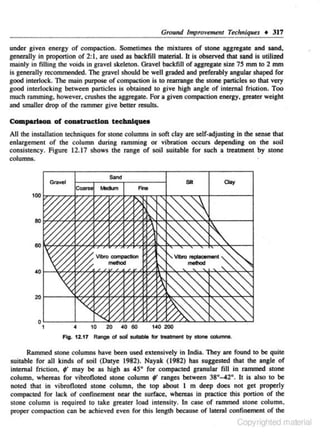
Analysis of granular pile foundations for triangular grid of piles show that s ignificant
reduction in settlement occutS only if the spacing of stone column is close (sld S 4) and the
piles are insulled to fuU depth of consolidating layer. However, too close a spacing (sld s 2)
is not feasible from construction point of view. Thus. a stone column spaci'ng {s/d) of 2.~
is adopted for mQSt practical problems. Also it has been recognized that closer sp:~Cing is
preferred under isolated footing than beneath large rafts (Greenwood. 1970).
LoU CU'f7IDC capacity of I.Dd1Yldu.l etoae columna
A stone column is subjected to a sttess condition much alike that imposed in the standard
triaxial '"t as shown in fig. 12.22. A vertical stress, <J, is applied by surface loading, aod a
radial effective suess. <J, results ftom the horizonllll reaction of the ground. Therefore, the
factors which govern the soik:olumn behaviour are (Hughes et at.. 197S):
-- ••
--{
- - :•
•
•
-~
--·
--·••
•
••
.--
•
•
•
~-
•
•
•
,- •
~-
...
"'
,:..,Y.!!!JI
• ~
•
Ag. 12.22 Slresses acting on stone column.
Copyrighted material

346. 322 • 'n1eory and Practice of Foundation Design
(i) undrained shear strength of the soil,
(ii) in-situ lateral stress of the soil,
(iii) radial stress--strain characteristics of the soil,
(iv) initial column
dimensions~
and
(v) streSs-str.lin characteristics and angle of internal friction, .-. of the column material.
The maximum vertical effective stress; on me column CJ.,/. is reached when the soil fails
radially. that is. the maximum radial stress it can develop. CJ,p is reached. It is generally
considered that the bulging in the stone column occurs over a depth of four to six times
diameter of stone column. An average depth of four times the diameter may be used for
obtaining the failure load.
1be relation between the vertic-al and radial stresses at failure is given by.
1 +sin;'
0
The value of o1
can
of • I
sin''
0
"
be expressed in tenns of the initial radial StreSS,
a,
=
(12.6)
o,. as
(12.7)
aro - u + Kc.
From Eqs. (12.6) and (12.7},
o1 =
where
1 + sinf'
_ .._, (o,.- • + Kc,)
1 - SlR.,.
(12.8)
c, is the undrained shear strength of the clay,
o,.
is the initial total radial stress.
u is the
pore~pressure.
f
is the angle of internal friction of the material of the column, and
K is an earth pressure coefficient.
Measurements carried out by Hughes and Withers (1974) in soft clay using a selfboring
pressuremeter (Camkometer) yielded K values of about 4.0, whereas Menard had earlier used
a conventional pressuremeter to obtain values of about S.S. 1be fuU·scale loading tests on
stone columns performed by Hughes et al. (1975) at Canvey Island confirmed the n:liability
of Eq. (12.8) as a design tool and pmposed a K value of 4.0.
Both limit analysis (Hughes and Withers, 1974) and field experience (Thorburn 191S)
suggest that the allowable vertical stress on a single stone column may be obtained from the
empirical expression
r1., =
2Sc,
F
(12.9)
where c, is the undrained shear stn:ngth of the clay in the region where the bulging of the
stone column occurs and F is the fac1or of safety (sometimes FS or Fs).
Typical design load of 200-400 leN per column is obtained for 900 mm diameter stone
columns in cohesive soil of undrained shear strength of 2S-SO lcN/m2 and a factor of safety
of 2.0.
It is interesting to study the deformed shape of stone column as observed after failure
by Hughes and Wi~rs (1974). Both field and laboratory investigations show geometric4lly
s imilar deformed shapes with bulging in the upper region, as visible in Fig. 12.23. 1be data
Copyrighted material

347. Hidden page

348. 324 •
17It!Ory
and Procriu of Foundalitm Dfiign
Settlement of atone column fCIUildationa
The settlement of stone column foundations consists of two components:
(i)
(ii)
the settlement c..-ontributcd by the soil treated by stone columns and
the seulemcnt contributed by the soil below the stone columns.
The settlement of the treated soil mostly occurs during loading by lateral drainage into the stone
columns while, the senlement due to the underlying suata occurs over a period of time
subsequently.
Behaviour of the ground reinforced with stone columns is a complex phenomenon. It
depends on various factors, such as the in·situ stress deformation and strength characteristics
of the soil and the stone flU. length and diameter of the stone column. and so on. All these
ractors are very much interactive and exact theoretical analysis is difficult. So design is
gencr.dly done. by empirical methods.
The settlement of a foundation on soft clay is caused primarily by consolidation of the
soil within the zone of influence. If the loaded area is large compared to the thickness of
compressible strata. as in the case of storage tank foundations. the immediate (e1astic~
settlement is sma11. The settlement of composite ground is ca1culated with the help of
modified expression using a settlement reduction ratio (Mitchell and KJ.tti, 1981). The final
settlement is obtained by adding the settlement of lower strata with the above setdement.
Thus. for a typical case of large area loading, shown in Fig. 12.25 (Som, 1995),
(12.10)
where
o = settlement of foundation
Pc1 = settlement of untreated soil within the depth of stone column treatment
Pcz = settlement of untreated soil below the stone columns, and
f3 = settlement reduction ratio for stone column treatment
Stone c:::dumn5
=
Hard sntum
6
• PPC1 • PC2
Pet = Settlement 0( slrirtum I
Pcz = Settlement of stratum II
{J
= Settlement Reduction tador
Fig. 12.25 Settlement of slone COlumn foundation.
Copyrighted material

349. Hidden page

350. 326 • Theory and Practice of Foundatiolt Duiglf
Maximum - - hydrclosl
6 centre = 255 mm
6R.
•250mm
6 edge = 150 mm
300
Fig. 12.21 Sflone column foundalion for large ClarneW llorage tarU .t Kandla: ae4llement
during hydnlleol
12.4 GROUND IIIPROVEIIENT IN GRANULAR SOIL
Numerous melhods of ground improvement in predomlnanUy cohesionless soil using the
principle of vibration are in practice today. Loose granular soil with 'N' less !han 10, is
characterized by low shear strength and low bearing capacity. In order to improve its
strength, lhe 'soil is compacted. This increases its relative density with consequent increase of
angle of shearing resisrance.
The compaction of soil is achieved either by repeated hammer blows on the ground or by
insertion of probes within the soil which are then vib<ated. 1be depth and extent of vibration to
be imparted depend on the nature of foundation problem encountered in a given situation.
12.4. 1 B-Y)' TampiDg or Drop Hemmer
The heavy tamping or drop hammer method of ground compaction employs repeated blows
of a heavy weight on the ground surface. In small works, a hammer (20-80 kN) is dropped
from a height of ~ m with the help of • driving rig or a tripod stand. 1be hammer is
made of RCC in lhe shape of a truncated cone with a low cenb'e of gravity. as shown in Fig.
12.27. The repeated blows of the hammer transmit vibration into ground which improves the
relative density of the soil in the upper layers and to a lesser degree in the lower layers.
Ramming is associated with gradual depression of the ground surface. With each successive
impact. the depression reduces in magnitude. After 5-10 blowS. it remains essentially
constant. The ramming is then continued in the adjacent areo.s. The ground is considered to
be compacted if the dry density of the soil achieves the following values:
S•ndy silt
15.5-16 kN/m3
Sand
16-16.5 kN/m3'
Copyrighted material

351. Growr.d Improvement Techn;que.s • 327
Flg. 12.27 COmpaction by drop hammer.
Ground improvement by the methnd of drop hammer is usually achieved in the top
2.5--3 m of the soil. Deep compaction is not possible by this methnd. This is clear from the
pre and post compaction density tests reported by Tsytovich et al. ( 1974) at a site in Russia.
wruch are presented in Fig. 12.28. The method is, therefore. suitable for small foundations
only.
13
0
0.5
14
18
Before
I
~
I
I
1.0
2.5
17
2
16
15
1
.
'
I
)
I
I
I
.....
r
1
I
I
After
c:ompacOicn
•o
I
3
Fig. 12.21 Oonsloy """"" e10p411 In c:on"4)adlon by drop hammer (Tsytcwleh. 1 974~
Based on experiences in Russia. Tsytovich (1974) suggested the depth to which s igoificant
improvement can be achieved by drop hammer technique. Table 12.2 presents compaction by
drop hammer in a tabulated manner.
Copyrighted material

352. 328 • 111rory and Practice of Foundation
D~sign
Table ll.l Compaction by drop h:unmer
O.p1h •I
ID~r conrpoctil)ll
Drop-weigh! rollen of 8 kN, 12 kN, 17 kN
Oouble-actin,g hammer. weighing 22 kN with a
lllOial bollom pial<
Hamroe~> 24 kN, dropped from a heishl of 4-S m
Heavy hammers weiJhin& 50-70 kN. dropped from a
(m)
1.0-I.S
2. 1
1.2.-1.4
1.6
1.6-2.2
2.7- 3.5
2.2- 3.1
helsh• or~ m
12.4.2 Dynamic CouoUdatlon
Dynamic consolidation is the name given to the procedure of deep compaction of soils by
repealed blows of a hammer falling from a height of 3()...4() m. The te<:hnique, pioneered by
Louis Menard, is used for compae1ion of soils 30 m below OL. Figure 12.29 is a
diagrammatic representation. of dynamic consolidation set up.
F1g. 12.2S Dynomlc -
·
Hammer weight used to perform dynamic consolidation in the field is many times more
than that used for heavy tamping. It may vary from 150-2000 kN. The shape of the contact
surface and the cross-sectional area of the hammer are chosen to suit the soil type and
reaction of the ground to the impact energy. Dynamic consolidation can also be done in
saturated cohesive soil provided the fonnation is varved and contains continuous sand
partings to faciliute pore-pressure dissipalioo. In homogeneous cohesive soil. dynamil:
consolidation may be done with pre-lnstaHed vertical sand drains to effect di-ainagc. as
depicted in Fig. 12.30.
Copyrighted material

353. Hidden page

354. 330 • Thtory and Practict of Foundntion Design
1000
Possibly
/
...foo
buildings
J
/
~
J
Unpleasant
J
-
/
I
10
100
1000
Sc:oloddlo..,.., ~EIO
Fig. lUI -
~
YOioe:i'Y _..,. -lmpect energy end
[E (ln J),
o (In m)J.
dlatance from lmpect point
12.4 .3 Vlbrocompactton
This is method of deep eompoction of granular soils where a probe is inserted into the soil
and then vibrated. Compaction is brought about by vibration, as displayed in Fig. I 2.32. The
process is essentially similar to vibnoftotation as adopled for installation of stone columns in
cohesive soil described earlier.
Water auppty
CoNslonless sol
(a)
(b)
(C)
flg. 12.32 Vit>rocompactiOn.
Copyrighted material

355. Hidden page

356. Hidden page

357. Ground Improvement Techniques + 333
has to be approached on a trial and error basis with past experiences serving as useful guide.
A suitable approach may be to
(a) carry out detailed soil exploration by conducting standard penetration tests or cone
penetration tests within the influence zone below the proposed foundations.
(b) determine the extent of improvement required in terms of increased Nor Nr value
from appropriate foundation analysis.
(c) choose the method of ground improvement, say, dynamic consolidation,
vibrocompaction. or compaction piles depe,nding on availability of facilities.
(d) select a representative area close to the consttuction site and carry out trial ground
improvement wortc varying the construction control parameters, such as weight of
hammer, height of fall, number of blows, spacing of compaction piles. and so on.
In genernl, the weight of hammer and height of fall are predetermined as per
equipment capacity. Before s"'Jting the trial ground improvement scheme, make
sure that predensification propenies of the soil, namely SPT, CPT da"', and so
forth are determined.
(e) carry out field tests to determine the post densification parnmeters after completion
of trial ground improvement work and determine the extent of improvement as a
function of spacing of compaction piles.
(0 choose the spacing of compaction piles on the basis of pre and post densification
data.
(g) carry out field tests to check the efficacy of compaction at different locations.
A trial ground improvement work has recently been done for the proposed construction of
a 120 m high temple obout 75 km from Kolka"'. The subsoil consists of a thin layer of firm
silty clay/clayey silt followed by a deep deposit of loose to medium silty fine sand to 25 m
below GL. Thereafter, a thin l•yer of stiff clay is found and the same is followed by dense to
very dense sand. 1be soil condition at the temple site is shown in Fig. 12.36. In view of the
high foundation loading anticipated from the temple structure. the ' sandy soil immediately
beneath the top silty clay 12- 14 m below GL required improvement.
Depth (m)
o ----~-=nm 7---.-.-.;~ da~d.---~~~~------------, A ~ ~~ ~~~~~~ 7.
N • 10
s------------------------------------------------II Loose to me<ium dense light grey
silty fine
N
s;~nd
with mlc:a
= 1~1S
12----------------------------·- -----111
Dense tlglt grey sllly fine sand
N= 30
~--------------------------------------IV Stiff to vetY stiff yellowish grey silty day
N= 20
30--------------------------- ------V
Very dense grey silly sand
N> 60
Fig,. 12.36 Soil condition at temple site.
Copy~ighted
material

358. Hidden page

359. Ground
0
10
0
2
lmprov~mem
Tuhnlqw~s • 335
N (biOws/30 em)
20
3()
~
~ 1'----..
' .... ....
/
............... IPool
....
---
Pro
10
''
12
;
Pile
Spacing
mx2n
~
<
15
(I)
5
Cone 10
2''
'~
X:'~
g
8
25
o-1.4 X 1.4
Pro
1
a ' ©+ -2x2
1
1
1
10
nee (MI'o)
15
20
fl
'2.8
X
2.8
~
12
~
1
1
1
(b)
Flg. 12.38 Results ol lrlol ground in'c><oYemonl
Example ll.J
A 22 m diameter x 15 m high steel storage tank is proposed to be built in a pon aru. The
subsoil condition is shown in Fig. 12.39. Preloading with sand wicks is proposed to be done.
Design a suitable preloading scheme and estimate the settlement of the tank during hydrotest.
Copyrighted material

360. 336 • Theory and Practice of Foundation Design
Tank 22m diame4et x 15m~
B«Mnllh grey silty dly. N • 2-5
c.• 30 I<Him'
U=60,R. • 25, w•35
CJ1 • eo • 0.06, C"el1 • eo • 0.010. Pc • 1~ kNim2
2m --------------------~--~----~I
N•1
c11 = 15 kNfmZ
U =65, R.•24, w= 50
CJ1 ·~·0. 18
7 m -------------------------------111 • Medium f¥WY lilly sandf..ndy ailt
N= 15
CJ1 + ., • 0.08
17m - - -- - - - - - - - - - - - - - N
Stllf y a i - brown sandy cloy:
N= 20
c., • 100 kNim2
LL =50, Pl =25. w=28
CJ1 • ., = 0.08
~m-----------------v Bluish gray slty aand: N • 30
C,/1 + ., = 0.05 (.......,..,)
3
7m-----------------Fig. 12.39 Subooil ooncl1lon (E>ample 12.1),
•
Sol.au"'
(a) Net foundation pressun:. considering 45• disper>ion of water load (140 kN/m2)
through compacted sand pad.
222
= 140 x 2 + (I.S x 20) (sand pad)
q,
(22 + 3)
= 108 + 30 = 138 kN/m2
Average c. of Strata I and
n
= ""'-' ;;.:;
(30_•_2)-::+:--"'( -·-=5)-"
1.:.5
7
= 19.3 kN/m2
q,,(n) = c.,N,
= 19.3 x 6 = 116 kN/m2 < 138 kN/m2
Copyrighted material

361. Hidden page

362. I
338 + Theory and Practice of FoundatWn Design
Stratum II
lip=
l!.c.
•
~
38
"
29.5
51
x 0.9 = 24.6 kNtm'
,
= 0.3 x 24.6 = 7.4 kN/m·
Hence, str<:ngth after hydrotest for
Stratum I : 30 + 30 + 9.5 = 69.5 kNtm'
Stratum II : 15 + 28.8 + 7.4 = 51.2 kN/m2
.
69.5 )( 2 + 5 1.2 X 5
1
We1ghted average of c. =
= 56.4 kN/m
7
q,.( n) = 56.4 X 6 = 338 kN/m2
FS = 338/138 = 2.5
(c) Settlement during pr<:load: Stage I
P, =SO kN/m 1
6
Layer
H(m)
I
2
11
5
Ill
IV
10
v
15
5
=""
L....
C, Hlo p, + llp
I + e.,
g Po
1
p, (kN/m'l llp (kN/m )
48
46
31
15
14
8
36
96
!56
236
c,
I + "<>
0.06
0.16
0.08
0.08
0.05
6 (m)
0.102
0.288
0.390
0.096
0.016
0.018
0.130
I 0.520 m
(• 520 mm)
Consider 90% consolidation of strata I and II, 30% in stratum III, and 10% in stratum IV
aod
v.
SeHiement at tank centre = (0.390
0.9) + (0.3
X
X
0.096) + (0.1
X
0.034)
= 0.383 m = 383 mm
(d) Settlement during pr<:load: Stage II
P, =50 kN/m2
6=
L 1 C,e
+
0
If log P.
+ llp
Pr~
Copyrighted material

363. Grou11d Improvement Tech11iques • 339
Layer
H(m)
I
2
s
10
s
II
Ill
IV
v
IS
Pu (kN/m2) t.p (kN/m2)
48
56
82
127
171
250
46
31
15
14
c,
1 + e0
0.06
0.16
0.08
0.08
0.05
6 (m)
0.031
0.152
0.183
0.076
O.oJ5
0.109
O.oJ8
l: 0.292 m
(* 290 mm)
Effective overburden pressure p. alter stag~ 1 pre~ has been detumined for full coosolldation under
the preload. ln reality. for s.lnlta Ill, IV and V. p. values would be less due to lower degree of consolidation.]
[Nou:
Consider residual settelement of stage l preload occuning in stage II and settlement for
s~age ll preload as
I 0%
30%
I 0%
Stage II : 90%
30%
I 0%
Stage I :
of stratum I and ll
of stratum Ill
of str.uum Ill and IV
of stratum I and II
of Stratum ll
of stratum Ul and IV
Settlement at centre = (0.1 x 0.390) + (0.3 x 0.096) + (0.1 x 0.034)
+ (0.9
X
0.183) + .(0.3
X
0.76) + (0.1
X
0.033)
= 0.262 m - 260 mm
Total settlement during stage I and slage II preload at centre is
383 + 260 = 643 mm
(e) Settlement of tank eentre during hydrotest: Ap = 38 kN/m2
6 =
Layer
H(m)
I
II
Ill
IV
2
5
10
v
15
s
L
C,
I + ~o
H log Pe + Ap
Po
Po (kNtm') Ap (kN/m2)
104
128
158
186
266
37
35
20
17
II
c,
I + 'o
0.10
0.16
0.08
0.08
0.05
6 (m)
0.026
0.084
0.04
0.110
O.oJ
0.095
O.Q25
l: 0.205 m
(.,. 205 mm)
(Nole give-n i n (d) abo..·e is valid for this case also.J
Copyrighted material

364. 340 • Theory atld Practice of Formdah'on Design
Total settlement during hydrotesl at centre of lank
30% of stage I preload (strata II), 0.3 x 0.096 = 0.029 m
10% of stage 1 preload (strata lii and IV), 0.1 x 0.034 = 0.0034 m
10% of stage n preload (strata I and II), 0.1 X 0.183 = 0.018 m .
20% of stage 11 preload (straw IIJ. IV, V), 0.2 ·x 0.110 = 0.022 m
90% of hydrotest load (strata I and II), 0.9 x 0.110 = 0.099 m
30% of hydrotest load (strata III), 0.3 x 0.04 = 0.012 m
20% of hydrotest load (strata IV and V), 0.2 x 0.055 = 0.011 m
= 0.195 m
<~ 200 mrn)
(f) Design of sand wicks
=
Diameter of sand wicks 65 mm. length
Take spacing at 1.2 em etc square grid
=8 m
- !!.,_ : J.l3 X J.2 =
d.
0.065
II -
20.9
For 90% consolidation, U = 0.9
Therefore, 1
ime foe1or, T90 = 0.7
Radial coefficient of consolidation, C, = 0.075 m2fday
Therefore, time for 90% consolidation (for 11 = 20.9 and T90 = 0. 7) is
190
=
=
T90
X
c,
•
d;
0.7 X 1.262
= 15 days
O.o75
Example 12.2
A steel storllge tank, 24 m diameter x 18 m high, is to
be founded on the subsoil shown in
Fig. 12.40. The formation level of the ground is to be raised by a 2 m sand fill prior to
construction. The soil is proposed to be treated by 0.5 m diameter stone column. Design
suitable foundation for the storage tank.
Solution
(a) The subsoil will be preconsolidaled under the load of 2 m sand fi ll with
preinstalled Slone columns accelemting the consolidation by sand drain effect. This
will increase the shear strength of the subsoil and also help in reducing
consolidation under tank load.
(b) The tank load (that is hydrotest load) will be dispersed through the sand padfsand
fill and the subsoil will be consolidated under the dispersed load during hydrotest.
The reinforcing action of the stone columns will help to increase the overall
bearing capacity of the soil and reduce settlement.
(c) Ground settlement under 2 m sand
nil
for 6p = 40 kNtml is
Copyrighted material

365. Hidden page

366. 342 • 17teory and Pracrke of FoundarU:m Design
(e) Be•ring capacity of tank foundation
Tank loading
E
Sand pad
Sand fill
E
"'
2
.
For 18 m h1gh tank, q,
= 180 X224
30
+ 2.0
= 135 kN/m2 ("'nd pad)
(f) Diameter of stone column = 500 rom
Spacing: 1.0 m c/c triangular grid
Area= 0.2 m2
Influence area = 0.866 ( 1)2 = 0.866 m2
02
.
Area rallo = _· x 100 = 23%
0 866
.
Olpacity of stone column
q,. =25c, =25 x 40 = 1000 kN/m 2
Using Eq. ( 12.8)
1 +sin;'
. .,, (a,.- u + K c,)
I - SID 'f"
= 4.26[(18
X
2 - 10) X 1.5 - 10 + 4
(GWT I m BGL. K = 4;
X
40) = 805 kN/m2
9' = 38°, and depth of bulging 2
m)
Q,1, per stone column = 0.2 x 805 = 161 kN
rJ
~11
Q.,, • -161 = 80.5 kN Say 80 kN
FS
2
per stone column = -
(g) Be3ring c•pacity of treated ground,
q~l
= [80 + (0.866 - 0.2)(6
X
50)/2.5]/0.866
= 188 kN/m2 > 135 kN/m2
Copyrighted material

367. Hidden page

368. 344 + Theory and Practice of Foundation Design
Barron, R-A. ( 1948), Consolidation of Fine-grained Soils by Drain Wells, Trans. ASCE,
Vol. 113. pp. 71&--734.
Brown, R.E. (1978), Vibroflotation Compaction of Cohesionless Soils. Joumal of
G.orec/rnical DivL<ion, ASCE. Vol. 103, No. OT 12, pp. 1437- 51.
Dastidar. A.G., S. Gupta, and T.K. Ghosh (1969), Application of Sandwick in a Housing
Projtct, Proceedings 7th International Conference on SMFE, Mexico. 2:. pp. 59-64.
Dastida.r, A.G. (1985). Treatment of Weak Soils--An Indian Perspective, Ceoteclmicol
Engineering, Vol. l, pp. 17?,..._229.
Datye. K.R. (1982), Simpler Techniques for Ground Improvement, 4th lOS Annual Lecture,
Indian GeotechniCGI Jounu>l Jan., 12(1 ): pp. 1-82.
Datye and Nagaraju (1977). Design Approach and Field Control of Stone Columns,
Proceedings lOth ICSMFE, Stockholm. Vol. 3.
Dhar, P.R- (1976), Soil Densijication by Compaction Piles at a Refinery Site, Symposium on
foundations and Excavations in Weak Soil. Calcutta.
Engelhardt, K.. W.A. Flynn. and A.A. Bayak (1974), Vlbro-replacement Method to Strengthen
Cohesive Soils in ..situ. ASCE NatWnol Structural Engineering Meeting, Cincinnati,
p. 30.
Greenwood. D.A. ( 1970), Mechanical lmprovem•m of Soil below Ground Surfau,
Proceedings Ground Engineering Conference. I.C.E., London. pp. 11- 22.
Hughes. J.M.O. and N.J. Withers (1974), Reinforcing of Soft Cohesive Soil with Stone
Column, Ground Enginuring. Vol. 7, No. 3, pp. 4~9.
Hughes. JM.O., NJ. Withers, and D.A. Greenwood (1975). A Field Trial of the Reinforced
Effect of a Stone Column in Soil, Geoteclrnique. Vol. 25, pp. 34-44.
Kjellman. W. ( 1948), Accelerating Consolidation of Fine-grained Soils by means of
Cardboard Wicks. Proceedings 2nd International Conference on SMFE, Rotterdam. 2:
pp. 302-305.
Mitchell, l.K. and R-K. Katti (1981), Soil improvement: Stote-ofthe-ort Report, Proceedings
lOth International Conference on SMFE, Stockholm, p. 163.
Nayak. N.V. (1982). Sum~ Columns alfd MonilOrbrg Instruments, Proceedings Symposium on
soil and rock improvement: geotextiles, reinfoit:ed earth and modem piling techniques,
Asian InStitute of Technology, Bangkok, December 1982.
Nayak, N.V. (1983). Struclurts on Ground lmprow!d by Stont Columns, Proceedings
lntemalional Symposium on Soil Structure Interaction. Roorkee, India.
Pilot, G. (1977), Methods of Improving -the Engineering Properti.s of Soft Clay, State-of-thean Report. Symposium on soft clay, Bangkok.
Copyrighted material

369. Ground lmprovemem Techniques • 345
Som. N.N. (1995). Consolidation Seulemt!.nt of Lorge Diameter Storage Tank Foundations on
Stone Columns ;, Soft Clay, Proceedings International Symposium on compression and
consolidation or clayey soils. Hiroshima, p. 653. Balkema Publishers.
Som. N.N. (1999), Stone Column Foundation for Lnrge Area Loading-Some Case StudieJ,
Symposium on Thick Deht,ic Deposits, Asian Regional Conference on Soil Mechanics
and Geotcchnicru Engineering. Seoul. Korea.
Thorburn. S. (1975), Building Supporred by Stabilised Ground. Symposium on ground
treatment by dee-p comp~c1ion, Institute or Civil Engjneen. London.
TsytOvich. N., V. Berezantzev. B. Dalmatov and M. Abelev (1974), Foundation Soils and
Substructures. MIR Publishers. Moscow.
Copyrighted material

370. Earthquake Response of
Soils and Foundations
13.1 INTRODUCTION
Earthquakes can cause extensive damage to foundations and structures built on them.
Earthquake motions are initiated in the soil and they are instantaneously transmitted to the
foundation causing adverse effect on lhe behaviour of the superstructure. Damage
may occur due to instabiHty of lbe soil which res-ults in extensive ground..movement including
differential movement. While structural damage is ultimately manifested in tilt or damage or
even collapse of the supenttuciUre, the initiating cause can often be identified as the advenc
response of the soil- foundation system under seismic forces.
Geotechnical considerations are. therefore, important in the development of an eanhquake
resistance design. It is not only the type of soil deposit that detennines the kind of response to
be expected during a strong earthquake. The type of structure also influences the seismic
response. The field of geotechnical earthquake engineering is quite complex. Much of its
applications are based on empirical studies made on the basis of case histories which illustrate
the effect of earthquake on engineering structures.
13.2 EARTHQUAKE CHARACTERISTICS
13.2 . 1 Magp.ltude
The most widely used magnitude scale to define the severity of an earthquake was developed
by Richter (1958). Accoroingly. the magnitude of an earthquake is given by the logarithm of
the ampliiUde on a Wood-Andenon torsion seismogram located at a distance of 100 km from
the earthquake source. Thus,
M = log(AIT) + /(IJ., h) + C, + C,
( 13.1)
where
II =amplitude in (0.001) mm.
T = period of seismic wave in seconds.
/(IJ.. h) = correction factor for epicentral distance (IJ.) and focal depth (h).
C_, = conection factor for seismological station, and
C, :a regional correction factor,
346
Copyrighted material

371. Earthquok Response of Soils and Foundations + 347
Natural seismic events may have magnitude as high as 8.5 or 9. Magnitudes below 2.5
. are not generally fell by humans. The frequency of occurrence of earthquake in a global
scale (based on observations since 1990) is shown in Table 13.1.
TabltiJ.I
Frequency of occu......,. of eanhqllllkes {since 1990)
Awrqe (Am~IN21)
lkst:riplion
a....
8 and ltighcr
I
Majo<
7- 7.9
18
120
820
S1r0ng
~9
MoclenJ!t
Uglll
Minor
Very Mlnor
S-5.9
4-4.9
3-3.9
<3.0
estimated)
6200 {
49.000 {estimolod)
Magnitude 2-3 about 1000 pet day
Magnitude 1-2 about 8000 pet day
13.2.2 Energy Release
The energy released by an earthquake has been related to the magnitude M by the equation
E = to•U+ts.u Joules
(13.2)
This energy is comparable 10 that of nuclear explosions. For example, a nuclear explosion of
one mega ton releases energy of 5 x 10" J. An earthquake of magnitude 7.3 would also release
the energy equivalent of one mega Jon nuclear explosion.
13.2.3 Intensity
The magnitude of an earthquake as obtained by the Richter's seale give s measure of the amount
of energy released by the earthquake, not its damage potential. The intensity of an earthqu'il<e is
a measure of the effect of an earthquake at a given location. Severa) intensity scales have been
proposed, the most widely used being the MIJ!Iiticd Mercalli Intensity (MMI) ~ale, as given in
Table 13.2 (Newmann. 1954). The value assigned to, tlje ·MMI scale gives qualitative
description of the damages based on physical verification at site. The equivalent value of the
magnillJde by Richter's scale is given alongside the MMI in Table 13.2.
Tabltl3.l Modified Mu,caiJi intensity (MMO scale (abbreviated vcrsioo)
lnu:nsfry
Ewlluano.
I
II
lnsigniftCMt
Very light
IU
up.
IV
Moderate
Slightly strong
Strong
Very suong
v
VI
VII
Ma&ni/11/k
(Richtu SC4le)
Only detected by instrumenL
s
On.Jy feh by sensitive persons.; osciU:Il:ion or twlJing objects
Small vibra""Y motion
Felt inJide buiJ
dings: noi.se produced by movina objects
felt by most pcr~s ; some panic; minor damages
Oam.ag.n to nonseismic resistant structures
}
People running: some damages in seismic resistant structures
and serious damages to nonreinforced tna$0nry s.t:ructures
1-1.9
2-2.9
3-3.9
4--4.9
~5.9
(Cont.)
Copyrighted material

372. 348 •
TJr~ory
and
Practlc~
of Foundation
D~sign
Table 13.2 Modifted MerealJi intensity (MMI) scale (abbreviated version). Cont.
MagniJud~
(Richur scalt}
'VUI
lksuucti,.·e
IX
Ruinous
X
XI
DisastrOUS
Disastrous in
extrtme .,
XII
C...S!roplllc
Sc:rious damacc: to structures in cenerat
Seriou.s dam~e to struc::turn: almosc tOCal desuuction of
nonseismic ttSistant $tNCCUJ'tS
. Only seismic resistant structures remain standing
l General panic; aJnlosc total destruction; the ground
cracks and opens
Total destruction
}
}
7-7.9
8-8.6
13.2.4 Ground AcceleratioD
The intens iry of ground mOtion during an earthquake is represented by the horizontal ground
acceleration produced. The predominant effect of an earthquake is the horizontal forces that
are produced in a s1rucwre. The horizon1al ground acceleration CL gives a measure of !his
force, which can be expressed by aw. (where W = weight of the structure) and acts at 1he
centroid of !he srructure. This horizonlal force· is depicled in Fig. 13.1. J.S. 1893 (1983)
gives the eanhquake zones of India bao;ed on the horizontal ground acceleration and the
vulnerability of an area to earthquakes.
aw
w
I
I
Flg. 13.1
Horizontal force due to ear1hquake.
13.2 .5 Respouse Spectrum
Response spectra arc typic.aJiy used to portray the charocteristic..~ of the earthquake shaking at
a site. Response s pectrum shows the maximum response induced by the ground motions in
damped single degree-of-freedom struclures of different fundamental periods. Each structure
has a unique fundamental period at which the SUIct.urc tends to vibrntc when it is allowed to
vibrote freely without any external excitation. The response s pectrum indicates how a
particular structure with its inherent fundamental period would respoiid to an earthquake
ground motjon. For example . measurement of ground motion in the 1985 Mexico City
eanhquake, response spectra shown in Fig. 13.2, shows 1ha1 a low-period srruc1urc (say,
T = 0.1 s) experienced a maximum acceleration of'0.14g, whereas a higher-period srructure
(say. T = 2.0 s) experienced a maximum acceleration of 0.74g for the same ground motions.
Copyrighted material

373. Earthquake Response of Soils and Foundations • 349
0.9
0.8
.
0.7
~
SCTsile
(depth to hard layer,
D"' 37m)
0.8
~
•
5% Damping
0.5
~
~
•
fi
o
.•
0.3
0.2
O.t
Rock and
..... SOil
3
Period (s)
F~
•
5
13..2 Acceleration response spectrum as recorded in Mallioo City earthquake, 1985 {Seed et al., 1987).
The response spectra shown in Fig. 13.2 illustrate the pronounced influence of local soil
conditions on the charac<eristics of the observed earthquake ground motions. Since Mexico
City was located approximately 400 km away from the epicentrc. the observed res~nsc at
rock and hard soil sites was fairly low (that is, the speclnll accelerations were less th~ O.Ig
for all periods). Damage was correspondingly negligible at these sites. At the Central Market
site (CAO). spectral accelerations were significantly amplified to 0.3-Q.35g at periods of
around 1.3 s and within the range 3.5-4.5 s. Since buildings at the CAO site did not
generally have fundamental periods within these ranges. damage was minor. The motion
recorded at the scr building site, however. indicated significant amplification of the
undertying bedrock motions with a maximum horiz.ontal ground acceleration (the spectral
accelemtion at a period of zero) over four times that of the rock and hard soil sites and with
a spectral acceleration at T = 2.0 s over seven time.c; that of the rock and hard soil sites.
Major damage including collapse, occurred to structures with fundamental periods ranging
from about 1 s to 2 s near the SCT building site and in areas with similar subsurface
conditions. At these locations. lhe fundamental period of lhe soU aJmost matched with that of
the overlying Sln.IC·tures. creating a near resonance condition that amplified the shaking and
caused heavy damage.
The Uniform Building Code of USA (UBC. 1991) recommends the response spectrum,
shown in Fig. 13.3. to determine the peak ground acceleration for a given fu ndamental
period T for different soil conditions. For T > O.S s. ground acceleration for deep soil strata
is considerably higher than that for rock and hard soils. It is to be no<ed that the period of
ground motion at a particular site is important in determining the effect of earthquake motion
on the structure. lf the fundamental period of a building is close to that of the site. a
resonant condition is created. This amplifies the shaking and increases the potential to
damage.
Copyrighted material

374. Hidden page

375. Earthqull.U Response of Soils and Foundations • 351
subsidence of 1.4 m. A combina&,ion of 1.3 m settlement of rock due to tectonic movement
and 1.3 m due to compaction of overlying soil led to a ground settlement of more than
After
'
..
·.
;
.. ·..
463.5'
Ftg. 13.A
..
.'•
...
Ground set3ement around well casing at Homer in AJaska earthquake 1964 (Grantz el al., 196A).
2.6 m at Ponagc in the same earthquake in Alaska. This caused widespread flooding in the
lltea during high tide· periods and the town had to be relocated at a new location. Similar
subsidence was noticed in other earthquakes also and the data is given in Table 13.3.
Table 13.3 Ground subsidence due to urthquake
Eonh.quaU
Homtt, Alaska
Portage. Ala~;ka
V alidina. Chile
Niigata. Japan
Ytar
t%1
t964
1%0
1%1
Rock ~ubsld~nc'
(Tectom'cJ (m)
Ground ~ubslden«
0.6
1.4
2.6
1.3
1.8
(m)
2.8
3.0
Ground se1tlement due to compaction of granular soil often leads to differential
settlement of sln.lctures. A differential movement of more than a metre was noticed between
a railroad bridge abutment, founded on deep piles. and the backfill placed directly on the
ground surface during the Niigata earthquake of 1964. This is shown in Fig. 13.5. The
bridge abutment, being founded on piles did not undergo much settlement but the granular
backfill experienced major subsidence due to compaction by seismic vibrations. Field
measurements have shown that vibrations induced by earthquakes are often responsible for
c.ausing significant struc tural damage resulting from differential settlement in a building
frame. Field observations of earthquoke induced settlement in saturated sandy soil are
summarized in Table 13.4.
Copyrighted material

376. Hidden page

377. &lrtlrquake Response of Soils (lnd FcundatiOII.S • 353
Fig. 13.6 Liquefaction In Nllgat& earthqvake, 1964
(O~ki.
1966).
Liquefactjon is caused in sand by ground vibration which tends to compact the sand and
dec-rease its volume. Jf drainage does nol occur, the tendency to decrease in volume resultS in
increased pore water pressure. lf the pore pressure builds up to an extent whic.h i.s equal tO
the overburden pressure. the effective stress becomes zero and the soil loses its strength
completely and gets into a liquefied state. Liquefaction may be initiated at the surface or at
some depth below the ground surf:Jce. Once liquefaction occurs a1 some depth. the excess
pore.pressure tends to dissipate by upward flow of water which. in turn. induces liquefaction
in <he upper layers of !he soil.
Copyngilteu r'lai nal

378. Hidden page

379. Earthquake Response of Soils and Foundations • 355
Ground aurface
.!,t..~=A
(1(1
(10
1_......._,
A • • · If water table
Is at dOp4h h
a - u0
wa..,
A • 2a, if
table
Is at surface
1cr = 8(1
(a)
0.7
li
• liQuefacliM
0.6
•No- •
~
o.s
•
,: o...
2
'
'"'
•
• •
0.3
lquofadlon
0.2
•
0.1
o
10
20
30
0
•
0
•
••
•
o«~
•
0
••
0
0
50
Appa~$~11 ...-
eo
10
density,
eo so
o, (%)
••
100
(b)
Fig. 13.1 Field obMMtion of lquoladion (Bymo, 1978).
0
10
Low possitMiity
of llquo-
3.0
20
6.1
a. 30
9.1
g
g
"
2:
High
<I()
ltQuefaciJon
"
a.
2:
possibility of
12.2
50
15.25
eo
18.3
Fig. 13.9 Relationship between lquelactlon potential and N valut: as a function o1 depth
(Kishlda, 1969).
Copyrighted material

380. 356 •
T1~eory
0.6
aud Praclice of Foundation Desig11
...
.---..,.--"""""!l.r,---- , - -- -,------,
"
~·
percent fines a 35
15
45
: I
o - - - + ----l!!-+--+-----+-----1
.sl
''
'
..
'''
'
''
:
''
''
o.•l----+- --+...-f--lft-----1----1
'
" ''
'
'
I '
...
I
I
I
I
I
I
I
' '
I
I
'
'
I
''
..
r-.conwnc
5%
McOfied dWieM o:de ~ Icily CICII'IIenl • 5,_J ..
........
No.
liqu!f!c:llii!?l u,..t!c!On Ugu!!.clialt
P~dalll
•
D
(Nolo.
Fig. 13.10 Uqoef.adion potential as
function d depth and standard penetration resistanc:e fol' different
percentages of fine• {Seed et al., 1984),
Based on this, a procedure for evaluaring liquefaction potential of a soil has
been proposed. The analysis involves detennination of average cyclic shear stress caused
by 1he earthquake and lhe cyclic shear scress required 1 cause liquefac1ion.
0
Seed and ldriss (1982) derived an equacion for obtaining lhe cyclic shear SlrCSS caused
by an earthquake. They considered lhe lime history of shear s1ress a1 any point in a soil due
to an eanhquake. A typic- l time history curve has an irregular distribution as shown in
a
Fig. 13.11. A wejghled average of 1he individual slress cycles gives lhe average shear scress
fav which is about 65 percent of the maxjmum shear streSS. Hence,
(13.3)
Copyrighted material

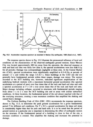
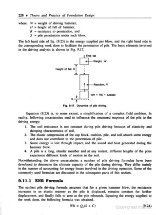
381. Earthquake Response of Soils (lltd Fou,dotions • 357
Fig. 13.11 Time history of shear stress during earthquake (Seed and ldriss. 1962).
where.
(...!...) ~.a=
g =
0' =
0
a~ =
=
r,
average cyclic shear stress developed during eanhquake,
maximum ground acceleration.
acceleration due to gravity,
total overburden pressure in the sand layer under consideration,
initial effective overburden pressure at depth under consideration, and
stress reduction factor ( 1.0 at ground surface to 0.8 at S m depth)
(refer Fig. 13.12).
·
r=~
04
.
05
(r
_
06
.
),
07
.
.
08
3
8
g
1
/
9
6
~ 12
15
18
v
/
/
v
/'
1.0
09
I
/
21
Fig. 13.12 Stre:s.s reduction factor
tot
liQuefaction analysis (Prakash. 1980).
For exampl e~ let us consider a site where the ground water table is at the ground surface and
a= 0.2 g. At a depth or S m, the average cyclic stress ratio during earthquake works out as
0 .29 (refer Eq. (13.3)].
Copyrighted material

382. 358 • Theory a11d Practice of
Foundatiot~
Desig11
The corrected N value at a depth of 5 m is 10 for clean sand with less than 5% fines.
From Fig. 13.9.
·
(_!_) = 0.11
qo
I
This gives.
(u:
- ~ > - ~)
(7~
I
Hence. liqutfaclion may occ.ur at the. site.
Table 13.5 gives the data on grain-size of the soil and depth of liquefaction in some well
known earthquakes.
Tabtt 13.5 Uqoefaction dala
Ltxati(Ht 1Jnd )YOr
Niigata. 1964
Mino-Owan. Jaq>ao. 1969
lallipan. Muico. 1959
Alaska. 1964
GI"Qirt-~iu
Mognitud' of
ttJffhqr.aU
7.5
7.4
6.9
D10 (mm)
O.Q?- 0.25
0.0$-0.25
O
.Ot-O. tO
o.ot-o. t
D<pth of
liqO(faaion (m)
s
9
7
8
It appears dlat liquefaction generally occurs in fine to medium sand within a depth of
10 m from ground surface. With increasing overburden pressure the chances of liquefaction
us ually decrease.
13.6
EFFECT OF EARTHQUAKE LOADING ON BEHAVIOUR
OF FINE-GRAINED SOn.s
Fine-grained soils such as sill and clay. have their engineering behaviour s ignificantly
affected by cyclic loading. The major influences of cyc-lic loading are:
• reduction of undrained shear strength of days,
• reduction of stiffness. and
• de•elopment of excess pore-pressure.
Undrained ohear
atrencth
Van Ee.kelen and Potts (1989) proposed a correlation. based on theoretical and experimental
work. between the postcyclic and precyclic undrained shear strength. Accordingly.
.,.
( )
cw -= 1-u,
c..
o;.
(13.4)
where,
C.,. = postcyc lic undrained shear strength.
c" = precyclic undrained shear strength.
11¥ = excess pore-pressure due to cyclic Joading,
Copyrighted material

383. Hidden page

384. Hidden page

385. Hidden page

386. Hidden page

387. Earthquake Response of Soils and Fouudations + 363
approximate distribution~ as shown in Fig. 13.16. decreasing from a maximum at the top and
zero at the base. The potential damaging effect of a base motion may be considered 10 be
proponional 10 the product of the force developed and the period for which it sets, that is,
Acceleration disb1bu1ton
In ftrtt modi
Maximum induced lallet8l forces c
Ooolgn-lotea
lndllood/dosi~J~Ia-1
s.
ck
tat. ralio• S.Jk
Fig. 1S.16 Sdlemallc -ntolion ol first mode lotces oo building.
ws.
Potential damaging factor oe
T
cc WS,.
where.
s. = spectral acceleration aod
s. = spectral velocity.
Most building codes used for earthquake·resislllnt design require that buildings of a
given type be designed to withstand a Sllltic lateral force having a magnitude given by a
lateral force coefficient k times the weight of the building. The magnitude of the coefficient
usually varies with the fundamental period of the building, or the number of storeys in the
r
building. In general. the lateral force coefficient dec- eases with increasing values of the
fundamental period or increasing numbers of storeys. Thus, buildings are not generally
designed to be equolly resislllnt to the same induced forces.
13. 10 DYNAMIC PROPERTIES OF SOn.
In order to carry out seismic design of foundation in an ~hquake region. soil parameterS
required for dynamic analysis should be determined. The imponant soil parameters relevant
to eanhquakc design fonn a subject matter of this section.
Putl ele-slse cllatributlon
Figure 13.17 gives the liqucfac:tion potential of granuJar soil based on grain ~size distribution
as obtained from experiences of J"'SI earthquakes (Oshal<i. 1970). The grnin·siu distribution
of the soil may be determined by slllndard t.,;ts.
Copyrighted material

388. Hidden page

389. Hidden page

390. Hidden page

391. Earthq11uke Ruponse of Soils atttl Foundations + 367
Sob<tion
The cyclic stress ratio at a given depth during an earthquake is given by Eq. (13.3). For a
horizontal ground acceleration of 0.2g, the depthwise variation of cyclic stress ratio (t/a~)d is
calculated. as in Table 13.6. To calculate the effective stress, the ground water table has been
taken at I m below GL. Now, from Fig. 13.10, for silt content 3S%, the cyclic stress ratio
required to cause liquefaction for different N values is oblllined as
N (blows/30 em) :
I0
Tla;
20
IS
0.18
0.4
0.2S
With factor of safety of 1.2, the allowable cyclic stress ratio would be O.!S, 0.208, and 0.33
for N values of 10, IS, and 20 rc:spcodvely.
Table 13.6 Calculation or cyclic stn:s.s ratio
lk!pth btlow
GL (mJ
N (blows/
30 em)
6
8
10
12
14
16
18
20
a.,(kN/m2)
a~(kNim2)
(CI./a'J,
.
Il l
61
78
95
112
129
146
163
ISO
1.82
1.90
1.95
1.98
2.01
2.03
2.04
2.06
6
12
7
8
16
18
24
22
148
ISS
222
259
296
333
370
,,
0.97
0.94
0.9
0.86
0.80
0.76
0.10
0.65
(Tia;J,
0.230
0.232
0.23
0.221
0.209
0.200
0.186
0.175
Looking at Table 13.6. it is evident that liquefaction potential does not exist beyond a
depth of 14 m. Here, N value is greater than IS and (T/a~) is less than 0.208.
Above 14 m depth. T/!1~ should be greater than 0.2 to prevent liquefaction. This will
require an N value of 20. Hence. den.sification of the soH has to be done by vibrocompaction
within this depth.
Example 13.2
During an eanhquake, the maximum intensity of ground shaking at a site is 0. lg. The subsoil
consists of a 20 m deposit of sand (fines c<>ntent IS%) with SPT blow count of 10 blows/
30 em. Determine the tone of liquefaction (Take = 18 kN/m 3 and water table at ground
surface).
r
Sol..,ion
(a) Average shear stress in the soil
T,; = 0.6s(a~ )("~)r,
Cfo
g
a(J
The calculations give
Copyrighted material

392. 368 • Theory a11d Practice of Fo1mdorion Design
l'able 13.7 Calculation of cyclk suess ratio
a_tg
a.,(kNim2)
a;(kNfml)
0.1
/kpth (m)
54
108
162
216
270
324
378
24
48
3
6
9
12
15
18
21
'fla~
'•
0.98
0.96
0.94
0.85
0.74
0.64
0.60
72
95
120
144
168
0.143
0.140
0.137
0.124
0.108
0.094
0.088
(b) Shear stress ratio causing liquefaction (see Fig. 13.10)
For N = 10 nnd 15% fines
T
':
a.
= 0.15
with FS = 1.2
.15
(.!£..)"' = 01.2 = 0.124
a:,
The da1a are plotted in Fig. 13.22. It is seen that liquefaction potenlial exists in the top 12 m
of 1he deposil.
0.09
0.1
0.11
0. 12
0.13
3
I
6
g
------ -- . . -- -----/
15
18
/
/
9
112
0. 15
0.14
0
/
v
. ./.':
/
------
--·---
.
21
Fig. 13.22 Zont; of liQuefaction.
Copyrighted material

393. &nhquake R<spons. of Soils and Foundations • 369
Ambreseys, N. and S.K. Sarma (1969), Uquefaction of Soils induced by Earthquakes.
Bulletin of the Seismological Society of America, Vol. 59, No. 2, pp. 651-664.
Byrne. P.M. (1976) . An Evaluation of the Liquefaction Potential of the Frazer Delta,
Canadia11 Geotech11ical Journal, 15, No. I. pp. 32-46.
GrantZ, A., G. Aafker, and R. K.achedoorian, (1964).-Aia.rka's Good F'ridoy Earthquake.
March 27, 1964, Geological Survey. US Dept. of Interior. Circular 491. Wa.<hington.
DC
IS 1893 (1983). Code of Practice for O.sign of Earthquake Resistant Structures, Bureau of
Indian Slllndards, New Delhi.
Ishihara, K. and S. Yasuda (1980), Cyclic Strengths of Undisturbed Cohesive Soils of
Western Tokyo, lnr. Symp. on Soils under Cyclic and Transient Loading Swansea.
A.A. Balkema. pp. 57-66.
Kishida, H. ( 1969), Damage of Reinforced Concrete Buildings in Niigalll City with special
reference to Foundation Engineering. Soil and Foundatiotr Engin~~ring. 6, No. l ,
Tokyo. Japan.
MarsaJ R.J. (1961), Behaviour of a Sandy Uniform Soil duritJg tltt Jalllpan EartlrquaU,
,
Mexico, Proceedings Fifth International Conference on Soil Mechanics and Foundation
Engjneering. Paris, France.
Matsui . T., H. Ohara. and T. Ito (1980), Cyclic Stress-Slr.lin History and Shear
Char.teteristics of Clay, Journal of tire Geotechnical &ginuring Division, ASCE. 106,
No. 10, pp. 1011- 1020.
Newmann, N.M. (1965), Earthquake Effects on Darns and Embankments, Geotechnique.
Vol. 15, No. 2. pp. 139-160.
Ohsaki, Yorihiko (1966), Niigalll Earthquake 1964-Building Damage and Soil Condition,
Soils and Foundalions. VI. No. 2, pp. 14-37.
Oshaki, Y. (1970), Effects of Sand Compaction on Liquefaction during tbe Tokachioki
Earthquake, Soils and Foundotions, Vol. 10, No. 2, pp. 112-128.
Prakash, S. (1980), Soil Dynamics and Machine F'oundotion, Sarilll Prakashan, Roorkee.
Rao, K.S. (2001), Magnitude Scales and Related Issues of Earthquakes, IGS News, Vol. 33,
·
No. 3-4, Indian GeOtechnieal Society, New Delhi.
Richter, C.F. (1958), Elementary Seismology. W.H. Freeman, San Francisco.
Ross, G.A., H.B. Seed. and R.R. Migliaccio (1969). Bri~ge Foundation Behaviour in Alaska
Earthquake. Journal of the Soil Mechanics and Foundations Division, ASCE. 95,
No. SM-4, pp. IOOT-1036.
Seed, H.B. (1968), Landslides during Earthquake due to Soil Liquefaction. Journal of tile
Soil Mechanics and Foundotions Division. ASCE. 94, No. SM-5, pp. 1053-1122.
Copyrighted material

394. Hidden page

395. Construction Problems
14. 1 INTRODUCTION
Foundation design is made on the basis of available knowledge about the structure to be built
and the subsoil condition available at the given site. The structural design is done in a way to
suit the facilities to be created for a given architectural layout. In general, the loads that arc
imposed on the soil can be evaluated fairly acc~ly. Foundation design requires evaluation
of the safe bearing capacity and settlement, both immediate and long term. These factors
require knowledge of the subsoil characteristics which are determined from an appropriate
site investigation. However, soil being deposited at a site by natural geological processes over
long periods of time, there are inherent variations which may not be fully reflected by even
an elaborate subsoil investigation. Hence, simplifying assumptions are made about boundary
conditions and average soil properties are to be assigned to the different strata for working
out the detailed design. Also, the land use pattern of the area surrounding the site determines
the vulnerability of existing buildings. Different degrees of precaution are to be taken to
implement a given design withoot causing any dist:ress to adjoining structures. The job of the
foundation engineer does no~ therefore, end at prllduclng a design only. It is equally
important to determine if any problems are 10 be anticipated during constriJction and work
out proper conatruction procedure and remedial measures in time.
The construction problems vary widely and are often site specific. However, some
general problems associated with foundation construction are discussed in !hi$ chapter.
14.2 COIDION CONSTRUCTION PROBLEMS
When a foundation design has been finalized, tho job is given 10 a con&tnJ<:tion agency for
doing the constnJ<:tion. Inevitably tho work requires excavation of varying depth and
magnitude. The problems multiply when excavation is to be made below the gmund water
table. The major construction problems, therefore, arise u a result of
I. stability of excavations.
2. dewatering. and
3. effect of adjoining structures.
571
Copyrighted material

396. 37'2 • Tlreory and Practice of Fo,ndation Desigll
14.3
STABILITY OF EXCAVATION
Excavation is done manually or by mechanical scrapers dependjng on the magnitude of eanh
work involved. Manual expansion is mostly adopted for foundation construction. Use of
mechanical scropers gives faster progress but they are not suitable for excavations in small
areas since the ramp roads needed for the scrapers to move in and out of the cut need space.
Mechanic.al scrape.rs are best suited to large area of shallow excavation.
Depending on the availability of space surrounding a construction site. an excavation with
side slopes or broced cuts may be adopted. Sloped excavation only involves earth work for a
stable slope designed from appropriate slopC stability analysis. Fi,gure 14.1 depicts excavation
with side slopes. But a stable slope needs sufficient free space in the vicinity of the construction
area. ln particular. if there are existing buildings c lose to the area. exca,•ation with s ide slopes
does not become feas ible. The.refore. in build up areas, braced cut is adopted.
Grct.nd
Fig. 14.1 ExcaVlldon wflh -
-·
81'11Ced cuts essentially consist of making vertical walls in the soil and suitJibly propping
them by steel struts as the excavation is done. When the final excavation level is reach~ the
foundation is cast and backfilling done to restore the original ground s urface as the struts are
progressively removed, as presented in Fig. 14.2.
Ground,._..
1 strut
st
2. 1 SMB 500 - - l
=
2nd strut
2. t SMB 600=--i
r-----------,
I - ----.. - - - - - . . 1
OIWall -
-->1
I
II
11
:1
11
,
II
..
3td Strut
2.1SMB600
1I
I
~
1I
t
1
~
____ , I I, ____ .,1l1 N cBo"::'a.rt levet
~
Fig. 14.2 Bta<ed cut.
Copyrighted material

397. Construction Problems • 373
For · shallow footings and raft foundations. the depth of excavation seldom exceeds
2 m and elaborate support is J>Ot required. However, if heterogeneous fill exists
near the ground surface. sjde protection with timber planks and small suuts should be
sufficient.
Deep excavation for two or three basements (excavation depth: ~10 m) would require
adequate lateral support with diaphragm walls or contiguous bored piles and struts. Because
of large excavation width, it may not be feasible to have horizontal struts which would tend
to deflect under their own weight. In such cases. inclined props supported between the
diaphragm wall and the already cast base raft at the centre may be adopted. Otherwise, a
number of H·piles may be driven at close intervals and the struts be made to span among
them to reduce the effective length. Figure 14.3 depicts inclined props to support diaphragm
wall and Fig. 14.4 shows struts in wide cuts.
lAgend:
1. Dlap!Vagm wall
2. Exc8Yation a b c d
3. C..StbaiO slab
4. Put Inclined struts
e
5. E>o:IVollon up to ~ ...,u
6. cast balance base slab
7. Erect wal lhrough ' " " '
Fig. 1"-3 Inclined propo to -
Strut 1- - '
clophracJn ..,.._
Slrut2 ~
Strut 3
1950
Fig. 1ol.4
Struts In wfde cuts.
Copyrighted material

398. 374 + Theory and Practice of Foundation Design
14.3 . 1
Design of Braced Cuta
The design of braced excavation involves two distincl yet intemlated features~ namely
'
(a) stability of the excavation, ground movement. control of water into the excavatjon,
effect on adjoining structures, and so on and
(b) design of structural elements, lhat is, diaphragm wall or sheet pile, struts or anchors
and so forth.
.
Although the overall s tabillry of braced cuts in soft ground does not depend to any
great extent on the number and spacing of struts or anchors~ lhey very much influence lbe
pattern of ground movement expected in a given situation. The depth of diaphragm walV
sheet pile determines both the slllbility of the system and the ground movement associated
with it. Depending on the subsoil stratification, one may get adequate Slllbllity against bottom
heave by having the diaphragm wall exteruled to a stiffer layer existing no more than a few
metres below the cur depth. However. this may not give adequate fixity to the diaphragm
waH to minimize ground settlement.
The essential featur"s of the design of braced cut in soft ground are discussed in the
subsequent subsections in details.
Depth of dlapbnpl wall
There is no established procedure for determining the depth of diaphragm wall below the
excavation. In homogeneous clay. not much is gained by !liking the diaphragm wall below a
critical depth. which is given by
N'- YH
c.
(14.1)
where,
r-=
unit weight of soil,
c. = undrained shear strength of soil below the cut. and
N, = slllbility number (" 6).
The depth of sheet pile/diaphragm wall is often determined by balancing the moment at the
bottom strut leveJ due to active and passive earth pressure on either side of the wall. This
gives rise to extended depth of wall, particularly if tbere is no appreciable improvement of
shear strength within the depth of wall. On the other hand, it may be adequate to determine
the depth of diaphragm wall from consideration of bottom heave alone. If, in particular, the
shear strength of the soil improves within shallow depth below the bottom of the cut, it may
just be sufficient to take the diaphragm wall to the stiffer stratum. For the Calcutta metro
construction, 10-14 m deep cuts have been made with 600 mm diaphragm walls !liken to
only 4-6 m below the bouom of the cut to rest in a stratum of stiff clay or medium/dense
sand. as shown in Fig. 14.5 (Som. 1998). Where the diophragm wall terminates in c lay.
factor of safety against bottom heave may be determined from Eq. (1 4.2). taking into
consideration the fOntribu&ion of shearing resistance al the soil-waH interface. shown in
Fig. 14.6. A facto[ o f safety of 2.0 would normally suffice. Needless ro say, presence of
struts. whntever the number, does not contribute to safety against bottom heave.
Copyrighted material

399. Construction Probhms
F=
y,D, + r.D, +
c•• N, +
L:C.<H + D, + n, )/ n,
s
-2.0m
,~.Om
'""
1
O.Om
Stratum I
Desk:caled brOwniSh grey
clayey silt
-3.8 m
2
~.5m
~.Om
Stratum II
Dar1< ""y lilly day wilh
3
l
Deplh below ground
d~WOOd
-9.5 m
-11.0m
level in
~
Slago IV -11.5 m
soage V
375
(14.2)
!;r<H + D-: + D1>
-1.!:1m
Sligo Ill
t
meuw
-13.2m
· ;-.
-13.5 m
Ser.tum Ill
Bluiolo ~ ..ly day
of WI f..
~ -17.5. .
Yri1h kankar
- 17.2m
Stntum IV
Yellowjsh brown sandy
dayfry silt
Fig. 1U 8noced cu1 for Calwaa me1ro conSlruclion.
G.l..
c,.,
)I
!
H
c..
I
tI " !
- o f cui
•
I
I
IV
I
I
y,
I
I
I
' ' ,_
--
/
g'
'
/
'
o,
!
Fig. 14.1 Slalllllly agoml bOliOm ,...,. In stratified soil.
Number llDd IIJMICIDC of 8tnlte
Struts are required to prevent failure of the diaphragm waiJ in flexure and to mmmuze
la~ral deflection or the wall. The diaphragm wall and the soruos make up a rigid structural
system which prevent excessive ground movement. Obviously. greater the number of struts,
Copyrighted material

400. Hidden page

401. Hidden page

402. 378 • Tlreory a11d Practice of Foundation Des;gn
variation of ground settlement for the final cut level may be obtained from Peck's
normalized plot for braced cut with sheet pile suppons in different types of soil. as depicted
in Fig. 14..9. Different zones of settlement proposed by Peck are shown as zones ), II, and
ill for different soil conditions below the cut (Peck, 1969).
Distance from excavation
Maximum CklpU of excavation
IT""!i!A
I.O
•••
••
•
•
2.0
3.0
• .o
Zone I
Sand and soft to hold cloy
Zono II
Very 80ft to soft clay:
lmiiOd dep4h of clay below
excavation
Zono Ill
Very ., clay:
elgnlftcant deplh below -
of excavation
Fig. 14.1 GfOund settlement In bfaceCI OJt (after Peck, 1969).
14.4
DEWATERING
Dewatering is required for any deep excavation to facilitate consbUCtion of basements, power
houses, pumping stations. and so on. lbeoreticaiJy, any excavation below ground water table
would necessitate some kind of dewatering. However, low permissibility soils, for example,
clay and silty clay (K <
cmls) do not present much problem with seepage because the
discharge is generally small and elaborate dewatering is not required. For medium to high
degree of permeability (K > 10·> cmls), suitable dewatering scbeme has to be worked out.
tcr
The basic purpose or dewatering is to control seepage into the excavation either by
pumping the water out of the excavation or by lowering the water table sufficiently below
the bouom of the cut till the underground works are over. The extent of dewatering depends
on the subsoil stratification, presence of water bearing stratum. aquifer parameters, and insitu permeabiliry.
14.4 . 1 Rate
of Seepage
The first requirement in a dewatering job is to estimate the rate of seepage into the
excavation for a certain degree of dewatering. For this. the excavation is considered as a
large circular we.ll from which water is pumped out to affect the desired ground water
lowering. For a fully or panially penetrating well, as shown in Fig. 14.10, the rate of
pumping is given by the well equation.
Copyrighted material

403. Construction Problems
0
t
379
P.mpW0 or test wetl
p round surface
~I G<Ound surface
2rCU<VO
Orawdown
curve
-
Initial water
{_~~
H
1m-
Impermeable Pata
, ••• J•••l ••JpJ.l ••••••• t,
snta
R
----.1
(a)
Unconfined
aquifer
(b)
Fla. 14.1 o Olsd>lrge trom well$.
(a) Fully penetrating well [refer Fig. 14.10 (a)]
trK(H 1 - h 1 )
Q = log,(R/r)
( 14.3)
(b) Partially penetrating well [refer Fig. 14.10 (b))
(14.4)
where,
discharge from a fully penetrating well in an unconfined aquifer (m3/s),
discharge from a partially penetration well in an unconfined aquifer (m3/s),
coeffictent of permeability of soil (mls),
height of ground water above the top of aquifer before drawdown (m),
height of water in the well above the top of aquifer after d"'wdown (m), that
is, drawdown = H - h(m),
r = radius of well or equivalent well (m),
R = radius of influence (m), and
h, = penetrating of well below water Ulble (m).
Q=
Q, =
K=
H =
It =
Copyrighted material

404. Hidden page

405. Hidden page

406. 382 • 71uwry and Practlce of Foundation Design
Deep wells should be constructed in such a way that they can remove large volumes of
water without nllowing large quantity of soil to enter the casing. When the soil consists of fi ne
snnd and silt. a sand filter should be provided. Figure 14. 14 depicts the construction of such
deep wells. Deep weJI pumping invol'eS the following steps for the well to be constructed.
(i) Take sink cased borehole diameter 200-300 mm whose diameter should be greater
than that of the well casing nnd depending on size of pump.
(ii) lnsen inner well casing.
(iii) Provide perforated screen over the length where dewatering is required with 3.5 m
length of unperforated pipe below for collec.tjon of fine materials.
,M.,~~~W ''-'rRislog ... _"
· _ ,,...'
-
water
level
Mesh filter screen
Silt colectino in sump -
-
Fig, 14.14 Deep welts.
(iv) Place graded gravel between casing and outer borehole casing over the dewatering
length.
(v) Fill the space above the screen by soil.
(vi) Water is 1hen ·surged ' by a boring tool to promOfe flow of wat.e r back and fonh
through the filler and fines collected at 1he bouom are bailed out
(vii) Insert submersible pump.
Copyrighted material

407. Collstructiou Problems + 383
The filter is designed on the conventional filter criteria suggested by Terzaghi which is
(a)
D., (of filter)
0., (of soil)
<
(b)
4
D15 (filter)
o., (soil) > 5
(~il ity
(Piping criterion)
criterion)
For slotted or perforated pipes,
0,.5 (filter)
(c)
width or diameter
or hole
>1
to prevent soil loss through the openings.
wen polut
dewaterlu&
This consists of installation of a number of well points, usually I m long, around the
excavation. They are connected by vertical riser pipes to a header pipe on the ground which,
in tum. is connected to a pump. The ground water is drawn by the pump into the header
pipe through the well points and discharged there. The well points are installed at 1- 1.5 m
spacing, as shown in Fig. 14.15.
Collecting space
T
Original
lnleC ports 1o rtser pipe
water table
Rubber ball raised When pumping
and towered when jetting
......... f'kl
Well"'*''
Well point
(a)
Senated jetting nozzle
(b)
Fig. 14.15 WeD point dewatering.
The filter wells or well poinrs usually consist of a 1 m long screen, 60-75 mm
diameter surrounding a central riser pipe. The well points are installed by pus hing or jening
them into the ground.
Capacity of a single well point with 16 m riser pipe = 10 lirreslmin. (approx.)
The spacing of well points depends on the permeability of soil and the rime available for
affecting rite drawdown. The spacings normally adopted for different soil types arc ns follows:
0.75-1.0 m
Fine to medium sand
Silty sand of low permeability
1.5 m
Copyrighted material

408. 384 • Titeory
011d
Practict of Foundation Design
Well point dewatering is suitable in both fine and silty sands. In highly previous soil.
the spacing required to handJe the water may be too smaU and impractical. Well points are
not generally suitable for clays because of slow water seepage.
Well points can lower a water table to a maximum of 6 m below the header pipe. For
lowering water table to greater depth. multiple stage well point system may be adopted.
Under average conditions. any number of stages can be used, eac-h stage lowering the water
table by about 5 m. A typical set-up for a two stage system is shown in Fig. 14.16.
Multistage well point may be used for greater depth of dewatering but this requires additional
header pipe. additional pumps, and larger excavation width for the provision of berms.
Stage 1
Original grOI.Wld
-lill.. .. _.__.t.~t!!.~~.!!l.--·--·­
Ground level
Stage 2
•.,
·•·•.,
..-·· -···-···-···-·····-···
Separate pt.rnps provided
for each stage
Stage 3
.,. ""li.--- •.,
...•.•········~·•.
! ~·~C:.red ground
.
watet level
(a)
(b)
Fig. 14.1 & Mu1tistage dewatering.
14.4.3 Field Control
Though expens ive. dewatering often becomes a necessity for underground construction. The
instillation of deep wells or well points. including the pumps and the fuel cost to run them
for long periods of time almost interrupted. make them an expensive proposition. It is.
therefore, necessary to have a system which makes the most optimum use of the pumping
instillation. The following points should be considered during the p~:
(a) As far as possibJe. any deep excavation should be undertaken during the dry season.
The water t~ble is generally high during the rainy season and greater lowering of
· water table is needed. 1he natural dewatering that occurs due tO seasonal fluctuation
of water table should be considered in working out the construction sequence.
(b) The first stage of excavation up to the level of ground water table can be done
without any dewatering. Suitable berms may be provided at this level for
instillation of deep wells/well points before commencing further c.cavation.
(c) The rate of discharge obtained by using well equation gives only an indication of
the rate of discharge to be expected for a given drawdown. There is no need to put
all the deep wells/well points into operation right at the begimung.
(d) Initially a limited number of wells may be comntissioned and depending on fie ld
observation, further wells may by added· taking into consideration the gradual
excavation process. The number of wells required for a cenain depth of cut may be
installed initially. Funher. additions may be done as the depth of cut is increased.
(e) Adequate number of standby pumps should be available at site particularly when
concreting is in progress so that any pump breakdown may be compensated without
'loss of time.
Copyrighied material

409. Consl'ruction Problems + 385
(f)
The effect of ground subsidence on :adjacent structures due to dewatering should be
evaluated ond adequate precautions taken to prevent major damage.
14.5 LAND FILLING
ln many construction projectS, low lying areas are co be reclaimed co raise the formation level
of lhe ground. Even in an app•rently high ground. often there m pOnds and depressions which
h•d been filled up in the past. In general, except for large scale land reclamation, not much
attention is given to such landfilling. All kinds of materials, including garbage and rubbish are
used to fill up these areas. A few years after filling when grass has grown on lhe land, there is
no apparent indication of filling nnd problems arise only during construction. Any load bearing
fill should be done with care and all data pertaining to the filling, namely type of soil. method
of compaction. date of filling, and so on, should be properly recorded so that the relevan1 data
pertaining to the foundation design are available during design.
14.5.1
Cohesive Fill
Cohesive soil may be used for land filli ng in dry areas. Compaction is done in layers.
250-300 mm thick. with a number of roller passes to achieve the desired degree of
compaction. Prior to placement, the physkal properties of the soil. including grain-size.
consistency limits.• water content and the like should be determined. Soils with high organic
content and high expansive pOtentinl should be avoided in filling work.
n,e compaction char.tc.teristics of cohesive soil are determined in the laboratory from
the standard or modified Proctor Compaction Test. Representative soils from the borrow area
are tested to obtain the optimum moisture content (OMC) and the maximum dry densily
(MDD).
Most compaction specifications provide for fie ld compaction at 90-95% of MDD as
determined from laboratory compaction tests. figure 14.17 gives the typical compaction
curve for clayey soiJ. Higher compaction in the modified proctor test gives higher MOD and
lower OMC than the standard proctor test. The curve of dry density versus moisture
condition for zero air voids is superimposed on the proctor tesl data for the purpose of field
contrOl. It is generally a good practice to have the field moisture content slightly on the wet
side of the OMC to ensure that all void space.' of the compacted soil are filled wilh water.
lt may be noted here that not all soils yield the same type of compaction curve a~
shown in Fig. 14.17. Lee and Suedkamp (1972) repOrted lhe test results of 35 samples and
suggested four types compact ion curves that are shown in Fig. 14.18. They also gave some
guidelines for predicting the nature of compaction curve based on the liquid limit of the soil
(Table 14.1 ).
T able 14.1 Type: of compaclton curve
Uq11id limit of soil
Nolu" of compaction cui'Vt' (Fig . /4. 18}
30-70
<30
> 70
Type II and Ill
Type Ill and IV
Type I
Copyrighted material

410. 386 • 111eory ond Practice of Foundatitm
D~.sign
24
22
~
"'-
.,
20
18
:t
f
~
I
/"
16
g
,r
Zero-air-void
curve (G, • 2.7)
~
I:-
14
I
~
~
....
....
• Standard pmctor
12
.. Moclffied prodor
tO
15
20
5
Mobture a:wttent. w('4)
25
Fig. 14.11 Dry density versus moisture content tlla:llonshlp from Proctor tesl
Dry unft weight
'
''
Zero-air-void
CUM
Zero-alr-YOid
( ,,,curve
Type t: Bell-shaped 0<
Single peak
L__ _ ____,~Mols-
"""'""' (%)
(a)
L-----Type II: One and -
peob
"""'*'' (%)
(b)
Dry "'" welgnt
''
'
Zero-air-void
Zero-air-YOid
curve
',
curve
'
Type Ill: Double-peak c:urw
Moisture content (%)
(C)
Type IV: Oddly shaped CUM>
'-----·Mob-'
con"'"
(d)
(%)
Fig. 14.18 Typical moisture density relationships ol c:oheslve soil (after Lee end Suedkamp, 1972~
Copyrighted material

411. Co!lstructio" Problems • 387
h may however be understood that irrespective of the type of compaction curve. the
highest value of MOD as marked by point A should be taken for specifying the field
compaction parameters in cohesive soil.
14.5 . 2
Granular Fill
Granular soil, predominantly sand, happens to be the mos1 suitable material for land filling.
Well graded sand (D001D 10 > 4) gives good compaction when saturated and vibrated. These
give high bearing capacity and low settlement potential and sand appears to be best suited for
under water filling.
The compaction of granular soil is determined by the relative density, defined as
R =
0
t:mal( -
tmak
e
x
100%
(14.6)
emi"
where.
= maximum
void ratio under loose condition,
t'mi• = minimum void ratio under dense condition, and
t: =: void ratio achieved at site.
emak
•
In terms of dry density, the relative density can be expressed as
Ro
~(
Yot- <rt>mi• )((]'")""")
<r,>.,.. <r.>"". r,
(14.7}
where.
Y.t = dry density achieved in the field,
(y ).,., = maximum dry density as determined in the laboratory, and
4
(rJ)11Wa = minimum dry density as detennined in the laboratory.
For field compaction. a relative density of at least 80% should be specified. This can be
easily achieved by placing lhe loose sand in 300 mm layers, nooding it with water and then
compacting it with vi bro:~tory rollers to 250 mm thick.
Numerous buildings have suffered damages due to inadequate attention given to the
ground filli ng in the construction area. Som and Sahu (1993} report the collapse of a
4·storey building soon after construction near Calcutta. The building was supported on a
c,entral raft with two-.way interconnected strip placed 5.3 m below the ground which had
indicated a bowl·shaped profile sloping across the building. A diffc,rential excavation was
made 10 locate the foundation below the lowest point Subsequent filling on the foundation
put an overburden pressure of varying magnitude across tile building area. This caused a non·
unifonn foundation pressure varying from 16 tlm1 on western side to 11 t/m2 on the eastern
side of the foundation, as shown in Fig. 14.19. The factor of safety against bearing capacity
failure was only 1.5. This is believed to have led to significant yielding of the soil and the
building tilted towards the western race due 10 heavier stress concentnnion. Subsequent
consolidation settlement (the building collapsed almost 3 years after St.."lrl of construction)
appears to have led to further tilting of the building and an estimated angular distortion of
1186 occurred towards the western side as against a permissible angular distortion of ll300 for
Copyrighted material

412. Hidden page

413. Hidden page

414. 390 • 17ltory and Practice of Fou,dation Desigu
3
A-Sand and soft day and
average workmansnlp
e-Very soft to soft Clay:
limited in depth below base
of excavatlon
2
Vet'f soft to soft day. Great
depth below excavation
c-
• • (%)
H
A
Distance from the braced wall
H
Fig. 14.21
Influence zone in braced cut.
Time is the essence of underground construction. Fasrer the underground works are
compleled, lesser will be the problems of 5ettlemenL Deep excavation should never be kept
open for long periods of time as this invites additional settlement and damage to adjoining
stnlctures. Figure 14.22 shows the effect of Calcutta metro eoostruction on a building close
1s r---------~============~
nne (monl'ls)
16
20
2.
28
32
o~r-~T-~~~~~~
E
::l
19.8 m 0 C 8
i
A
6.5 m
120
J.eo
-~ ·---------
" - - Diaphragm -
L
Ayg. ol A , 8, C, 0
200L---------------------------~
Fig. 14.22 Effect of time on building settlement a<tjacent to braced cut.
Copyrighted material

415. Ccnscruccion Problt!ms + 391
to the diaphragm wall. For various reasons, the metro work was stopped repeatedJy at this
section and the construction took the best pan of three yean. The excavation was kept open
for 90 days at 8 m depth and thereafter for almost two years at 14 m depth. It may be
noticed that out of a total settlement of 172 mm, no less than 93 mm had occurred during
stoppages of construction. The data clearly show the effec.t of time on ground settlement
adjacent to a br>Ced cuL
14.6.1 Effect of Vibration
Vibrations caused by construction operations such as blasting. pile-driving. compaction by
drop hammer, compaction piles, and so on can damage existing structures and equipment if
not designed to resist such motions. The peak panicle velocity near a building due to a
source of single impact is shown in Fig. 14.23 (Mayne et al., 1982).
1000
~
.s
f
~
1!.
~
Pooolbly
/
unsafe for
buldlngs
J
100
v
Objection-
J
10
Unpleaunl
/
/
NoU<>eablo
I
10
100
1000
Sealed distance• .Jo!D
Fig. 1•.23 Partide velocity versus di$tanoe <Jue to a single rnpact (after Mayne et al.. 1982).
A safe upper limit for small buildings. is given as
O
.S6
v =
70 (
£,
IOD-
( 14.8)
)
where.
E = energy per blow in KJ. and
D = distnnce between the source and the structure under consideration.
A maximum peak particle velocity of 50 mm/s is normally considered safe for conventional
buildings.
Copyrighted material

416. 392 • 111e.ory and Practice of Fo11ndaJiOtJ De.sig11
If the vibration level is intolerable, the soil foundation system may be modified lO
minimize the effect of vibration. This may be done by providjng vibration barriers. Trenches
may be made around the vibration source for activ~ isolation or may be made near the object
to form pa.uiv~ i.wlalion. For active isolation. lhe depth of trench should be 0.6 times the
distance from the structure. This would reduce the ground motion to one quaner of the
amplitude of 'no lrench' condition. For passive isolation, a semkircular plan area behind the
trench at a distance LR with lhe depth of trench equal to 1.33L~ would give effective
isolation.
Lee and R.J. Suedkamp (1972), Charoct.ristics of ln·<gular Shap<d Compaction Curv.s of
Soils. Highway Research Record No. 381, National Academy of Seeing. Washington
DC, pp. 1- 9.
Mayne, P.W., J.S. Jones and R.P. Fedosick (1982), Su/J-surface Improvement du< to Impact
Dmsification. ASCE Geotechnical Conference, Las Vagas, Prepriat, Session B 2.
Peck, R.B. (1969). Braced Excavation and Tunnelling. State·of-the-art R<part. Proceedings
Sth International Conference on SMFE, Vol. 3. pp. 225- 290.
Soda. S. (2001), Offshore Artificial lslat~d Co~tstruction in Japan- Example of Offsltore
Airports. Proceedings 2nd Civil Engineering Conference in the Asian Region. Tokyo.
p. 77.
Som, N.N. (2000), Rectification of BuildU1g Tilt- An Unconventicnal Approach, Proceeding
Indian Oeotechnic;U Confereoce, Bombay. Vol. 2.
Som, N. and I.R.K. Raju (1989), Measuremenl of i~t-sltu lAteral Stress in Normal Calc.ulla
Soil, Proceedings 12th ln1
emational Conference on SMFE. Vol. 3, pp. 1519-1522.
Som. N.N. and R.B. Sahu (1993). Investigation of Co/lapS< of an Apartm•nt Building du< to
Differential FUiing. Proc. Third lnlemational Conference on Case Histories in
Geotechnical Engineering, Missoorie-Rolla, USA.
Copyrighted material

417. Appendix
(a) Venkal stress influence coeffic.ient for unifonn circular load
•
11+1~•~
II
1'..,-,
qlunit ..a
--~~~~-L--•
X
•
•z
•
·; .. • <r,l)
Table A.l
,j'g:
0
0.5
1.0
1.5
2
4
(b)
Values of / 0
0
1.000
0.910
0.5
1.000
0.790
0.560
0.375
0.258
0.083
0.646
0.424
0.286
0.087
1.0
1.000
0.417
0.332
0.256
0.196
O.Q15
Venical stress influence coefficient for uniformly distributed strip load
~.::.·-lqtunit ....
I II
!
X
•
:z
•
-,- ~ (r, Z)
z
(11
e ql11
Copyrighted material

418. 394
• Appendi:r
Table A.2 Vah»es or lv
dRa
0
0.5
1.0
1.5
o.s
0
1.0
I.S
2
0
0.09
0.25
0.27
0.29
0.28
0.26
0
0.02
0.08
0.15
0.18
0.20
0.22
1.00
1.00
o.so
0.96
0.82
0.67
0.90
0.73
0.61
0.51
0.40
0.30
0.49
0.38
0.45
0.41
0.30
0.25
2
o.ss
3
4
0.39
0.31
(c) Vertical stress influence coefficient for lriangular load
qfui'Wt area
•
•
•
•
••
X
--·;····•
1
z
(Z, X)
a,
= ql.
Tabk A.3 Values of lfS
~·
0
o.s
I
2
0
0
0.13
0.16
0.13
o.s
o.s
0.41
0.28
0. 16
I
2
0.5
0.35
0.25
0
0.03
0.07
0.08
O
.IS
Copyrighted material

419. Index
Aerial pbo<ognph" Y
Allowable lood on piles from SUIJc ..Wysis. 218
Allowable seulcmenl.
Boring. Y
auger boring, l l
n
percussion drilling. 36
rowy drilling. lli
Angle of shearing res.istance, tA
Apparml cohesion. I.A.
Approximate method of decerminin& venicle stress.
1.06
Allerberg limits• .S
Liquid limil, S.
Plastlc limiL. S.
Shrink~e limit. 5.
Band drains.
trial pits. l! .
wash boring. H
Broce<! cuu. i l l
Building dan'lq.e due to liquefaction. 360
Bulk d<nsity, '
Buoyancy ran, §J!. 1.21
Caissons, 266.
box. 266
open, 266
ll.Q
Ba.semem 1'1.1. 1&1
Beoring capacity, 1J!. UL 1.21
allowable.
pneumatic. 266.
Capachy of pile group. 224
Causes of defect in piles, 246.
!L 11m
from field tests. lll
of non·homogenoou.s soil. 121
Cellular raft. L8ll
Chemical And mineralogjcal d.ala. 6ll
Chemical injection and grouting, .Yl6
During capacity analysis
bearing capacity factors, W
depth factcn 126
Hansen's method. 1.26
inclination factors, 1.26
local shear failure, 1.26
Mcycrl>ors method. 1.25
Prandtl's analysis. 120
shope facton. 126
SktmplOn' s
Chemical tell on water samples. 6ll
Choice of foundation type. 10.
Class.ificatioa of sweJJing potential. 221.
Clay minerals. 2
Illite, 2
Kaolinite. 2
MornmorHionite. 2.. 22.5.
Coerlicient or earth prtSSu re at rest.
CoerfiCicnt of consolidation. 2S
method, 115
Ten.aghi's :malysis. l22
VC$ic's method. 126
Blad cotton soil, 22:1.
8ortd and cast·in·situ piles in cohesionle$.<> soiL 212
Bored piles. 2Jl1
in cohesive soil. lOS
1L
lM
Cohesive fill, l81
Combined footing. f& l.6!l
Common construction problems. lll
Components or well roundation. 268
bouom pl·ua. 2.62
w uing edge. 262
in cohesionless soil 205
595
Copyrighted material

420. 396 + f11de.T
dredge hole. 26!1
intermediate/top plug. 210
steining. 269
well cap, 210.
well curb. 269
Concrete piles. 200
Consistency. 6.1
Consolidation. 63
coefficient of. 2i
degree of, 25
rtue of. U
ConJOii<bliOn settk-ment. lA2
Conventional nlfl. 61. 11S
Critie>J depth. 216
Cyclic shear strtss. ~
Oam~c
limits
for load bearing walls. U
of angulu diSiortion. U
Damages due to diffetential seuJement. 22
:1Jthitecturul. 12.
combined structural and architectural, 23
$11l<turol. 12
visual effects. ll
Darcy's law. 12
Deep foundations:68
piers and caissons. 62
pile fou!Kbtion. 68
Ocgrtt of saturation, .1
Depth com::ction, lJ2
Depth
of boreholes. i2
of d'in..phngm wall. i l l
of fi dty. 2ll
or rootina. w
or penetrnlion. 376
[)esjgn criceria. 10.
Design (or equal settlement, U2
Design
of br>Ced cuts- 374
of. r:a1 foundation. US
Desigo parameten. 6J
Dewatering. 318.
methods of. 380
deep olltll pumpina;. 38 1
rickl oon110l, lM
sump pumping. 3SO
well point dewatering. 3.&l
Difflnntial free swell. l l i
Dimensioning foocina found3tion$.. 1.10.
Driven piles. 20.1
cast•in-situ. 2ill
in cohesionles.s .soiJ, 205
in cohesive soil. ~
Dry density. 4
Dynamic pro~rtirs of soil. 3§3
damping factor. 365
partkJe-sizc distribution. 3.63.
radi31ion dampin&. 365
rdative clt'nsity, 364
sbe.ar modulus. 364
DynAmics of pile driving (dynamic analysis). 2.1.2
ENR fonnula. 220
Hiley fonnula. lli
Janbu's formula. 222
limit:~lioos or dynamic analysis. 223
Simplex fonnula. 22.1
wave equation. m
E.nh pressure, 376
E.anhqum . l!l6
A lll>ka. lS.J
Bhuj, 354
ill
cntJ'ID' releaoe. l!l'l.
intensity, ::M1
m~ni tude or. ~
Niisata. 352.
modified Merc:alli Intensity. i l l
Rkbter scale, Y6
Effect of
adjoining SUUC:lwt:S, 31.1
eanhquake on fine~graincd soil.s, i l l
ground water table, l68.
ground water table oo bearing capacity.
~
swelling, ~
Cime on building settlement adjacent 10 braced
cut, J2D
vibrntion, l2.l
Effective stress parameters, 6l
Effects of eanhquake. 350
Efficiency or piJe group. 22!i
Elastic parameters. 21
Elastic th~ry. 152.
End bearing. 213
in cobesionless soli, 213
in cohesi'e soil. 213
End bearing piles. ~
Engineering propcrtie$. 60
o( soil. 12
Expansive soils. Ul. 226.
Factors affeeting bearing capacity, 122
Copyrighted material

421. 111dcx •
Fallu~< mechanism,
U!
GrouNI improvement In cranulat soU, J26
w
__....piles. 332
coocro1 or fidd WO<t. 332
dynamic coruoi•dallon. m
ccncnJ .,....., failure.
1oco1 • • r..~m<. ta
punchin& • • foil=. 111
F"~<ld
conuol for pn:loadin&. lll
f ' o d c l - - fa< prcloodooc. ll.Q
lidd I<Siin& or IOils. 40
dim:t she• ,... (ln·litu). tl
dynamic cone penetJ ation ltst. !3:
Menard pressuremeu:r, 49.
plate burin& OtSI. !18
~- 4!
SIIDdardpct..badooOtSI. 41
-
obi"' in expons~~ 1011.
d1<mleal
CNS layer. Jll.l
c:ootrollinl swellina. 300.
,...,m-. m
m
aurdlata< loodinr,. 3W
under-reamed piles. 2!1.8
Foundations
deep. 6l. 6&
..,ca.y. U&
,.n or mil. 61
shallow, 66
Frtt-sweU teSt. ~
Friction pila. 200
F'iidiooal fHtPMW"e. 206
in cch<sionleu soil. 210
in cohesive soil, 2D1
Fuodamcntal period. l:i2
GcoloP<aiiWV<l' tepOIU .... . . _ y
Oc<>phys>Cil - - y
Orain-siz.c d1mlbution. 1
Onmular nn. l81
Granular soil
Honeycombed suvcture, 1
LS. code 2Ml
lrnmcdi... ldll<JO<tO. w
lndlan Randud ctwlncmion syau:m. 8
lnllucn« of ....,.poll>. u.&
lnlluentt zoot in bnccd cuL liD:
I......,...,W.~ IS
l -. t l
Jtolll<d roo11nr.. ~ ~IoA
Llbonta<y 1<$1 ....... 60
Labanlo<y ...... 11
Locey' s silt ,....,, 2l1
l..lnd fil1ing. l&S
Lara• area loadina. 325
Lateral liability ot wells. m
llombaymcobod. llS
or. m
Gtoos ...S net sod ........,.., sofc beain& ~'Y·
llJ
Gross ultimate bearina capudty, 10
aceckr~cion.
..... o r - tt
Wa<madoo roquiml f,_ soil invad&- ll
ln-11tu compusibi.bty. 2S
1n-·siru stress. l6
lnteariCY ICSiin& of piJel. ~
lncerference dfm.. Ll2
... ....s. ll2
(iround
Ground treatment in cohtsive soil. ~
Ground waaer table, 1.1
0<-oolndw-. lll
Wlltf table. lQ
~--- lim
_....oowidulaodxa- m
SlrU<IIIrt
priftcipks or. Jill
Oround ldllcm<nl. 350, 377
aquifuJ<. II
aquitanl. lJ
capillary zone. ll
r<eharac. lll
l. JIIS
Foras Odin& .. well foundadoo. m
heavy tampina or drop hammer. 126
triiLIJround improvement. Jll
vibrocompaction. l30
Ground impvvc:mmt
aquif<f. IJl
Sialic cone pcnetr.rion tdt. U.
V aoe lhear test. ~
Flooting r da·ion. 11&
...
- - IWCOII<.
Jn
lil8
bulthcad_.,..m
IRCmcobod. llS
Layout and nwnbcr or bord>olcs. 51
Llmitatlons or lheorttJcal analysis. 129.

422. 398 • Index
Limits of consistency. 5
Uqu<Foctioa. 352
Uquefaction potential, 3!"4
Uquidity indt:x. S
load carrying capacity of stone column. 323
Load venus settlement n:l:JC
ionship, U1
Load te:s:l on piles. lli
constant r..1e of penetrntion (CR.P) test, lli
testing of. l l i
timber. 200
Pile sp::acing. 225
Piles unde- horizontal forces.. 2l2
r
Pistoa sampler. l8
Planning or exploration programme. S.l
Plasticity chart. 6
mainWned lo:ld test. 248
Plnsaicity index, S
Plme load test, W
procedure of. 248
Port·pre$SUte,
M.l."f. classification system.
1
Measurement of shea: strength. 1.8
Measures to prevent lique(ac:tion. 362
Mohr-<outomb eq~ion, ,J1
Movement of diaphrngm wall. 376
Negative skin friction. 242
day overlying sand fill, 243
neutral point. 243
sand fill ovtrlying clay, 244
Net pennissible bewing pm.s:ure, 1S
Net ultimate bearing capacity. ZQ
Newm:utc' s chan. &2.
Nonlinear soil, l1ll
Normal Calo.atta deposit. 2
Normally coasoU
dale<l clays. 23
Number :md spacing of suuts.. ill
Open drive samplers.. l8.
Organic soils, 9
Overconsolid:ued clays, 21
J.4
codfidents. L6
Porosity, 4
Pre-consolidation pressure. 2&
Prtkwl.ing with vertical drains.. l06
Preservation or samples. 32.
Pressure bulb. 2.1
Pressurt-void r:uio relationships.. 22
Principle or effective stress, 13
Radius of influence. lll. 380
Rammed stone column, lUi
Rale
of discharge, 380
or,..poge, ill
of settlement, W.
Reclaimed ground. 389
Reconnaissance study. l3
Relati'C density. 8
Response $pe<OUlll, Y8
Responsibility or designer. ~
Rigidity of footings: contaCt pressure. 92.
Sampling. l2
from boreholes. ll
from trial piu, 31
Peat. 2
PC'dologjeal data. l:i
Ptnneability. 12
Pennissible seulement. :U
Pile behaviour under uial load. 20J
Pile cap:acity from in~situ soil tests. 2!ll
Pile driving analyzer. 2il
Pile group subjec...'tcd to vertical Jood and mome-nt.
227
Pile groups, 223
in cohesionless soil, 1lQ
in cohesi ve soli, m
Piles, ~
in cohesionless soil, 205
in cohesive soil, 2n!
Sand drains. 30?
drain diamcter, Jmi
drain spacing. ln8.
cypes of vertical drains, 309
Sand wiclts, 309
Scour deplh. 21ll
Scmi-<mpiri<al mdhod, ~
Sensitivity of clays, 2.1
Setdement analysis
methods of, Ll2.
SctOement
of pile groups. 22B.
of stone column foundations. ill
Sentemtnt criteri:a. 11
Settlement reduction r3tio. ill
Copyrighted material

423. Shear .stren&.Ch or soils. U
Sil< owad....._ l2
- o f. Jl
s~ cxcavatton.
m
Sotl
aeolion, l
es<uorin<, l
Jlacial l
bocwtrin<, I
marine, l
l'<$idual, 1
oectimencary. 1
Soil c:lassifiCOlioa. 2
Soil dq>osiu o( India. 2!1
Soil profile, 9.
Soil .... cq>orc. 15
Stability or excavation. l22
SUobiliulloo ol bord!olcs. l6
by ....... l6
by drilli.. tluid. J§
by w..,., l6
Standard pe:neuatlon test, ~
Slade ealyAs. 2Ql
Sialic: oone 1a1. W
Sl<d pila. :zm
Slonccolums. ll!
Suess concencnlioo facto<, Jl'
Slt<SS diJiributlon In oon·homoJeneou.s aoiiJ, !lA
mulliloye< · - !1'1
~-- un
ri&id bose JYII<m, lY
sinJI< elutk: llytt on a rilld bose. 96
fhrte:..la:yer aySiems. ~
IWO laytta wilh cliff..... daslic ponmecen. !IS
'-laytt
lY
Stress inew~mcnt raio. W
•roc-
Slt<SSadu<cor.........,loodinc. l&
Boossinesq analysis: point load. 2&
embonkm<"' cype loadinJ; 8l
lriangular load, I§
t.miform line loed. 8S
uniform Jlrip lood. M
vertical SCMKs below uniform cin:ul.ar &o.d. ll
venicaJ acrcuc.s below uniform m:mn.a:ular load.
&J
Stresses du:rina loading and ~on in the
fidel. IJ6
Slt<SS-poch.
w
-
lllll)'lio. lll<lhod of, IJll
s.rip foobc>&. 61. l6f
SIIUCIIIrll apocicy or pileo. 196
Struc:naal design
Offoolinp. W
ofr>ftfOWIOIIIlon.. W
daale!Ddllod. W
riJid !Ddllod. W
S1n11 load, l18
SubmcrJed denslly, &
SW<UinJ pmsure, 296
TcstlnJ ol JOil. 40
clwifoadoni<StJ, Ml
en,inoerina proptttic.s. ~
~~JyJctm. l
Total oonu1 pr<SSift. lA
1)pa o( " " ' ' _ . . . , - . 3!2
Triulal ...._ I!
consolidated dralned 1<11. 2ll
consolidaced undrained ...._ l.i
- - - n e d - 1!
Ukllllllt lll<ral m ill...,., 2:1&
U....,_reamed plies, 194, 210
Undrained shear llreOJ1h. 112
o( days. 2!1. lll
Uooifoed JOil c:lassifoadon . _ a
Uolfonn ~ code of USA, lU
Uniformity coefficient.. 7
Unll wci&lot. t
Uo~oeciJW<II ...._ 2llS
Uplift oni11-n of poles. 231
Validity o( Darcy's law, U
v ibronOlllion. lU
Void ntio. &
wllef COftiCDl. "
W<lllhering. I
Well Fouoodalions. 266
Well liokiftc. 1&J
Wdvm- 6i
Copy

424. CopynQhled naler. '

425. Hidden page

426. Prentice· Hall of India

427. Hidden page