This document provides an overview of texture analysis in image processing. It defines texture as a feature used to classify image regions based on spatial patterns of intensities. Texture analysis involves both texture classification, which identifies textured regions, and texture segmentation, which determines boundaries between regions. Common quantitative texture measures described include range, variance, gray level co-occurrence matrices (GLCM), and gray level difference statistics. GLCM capture the spatial relationship of intensity pairs and various statistical features can be extracted from them, such as contrast and homogeneity. Problems with GLCM include how to select the displacement vector. Texture analysis algorithms typically operate within a window across the image.

1. Michael A. Wirth, Ph.D.
University of Guelph
Computing and Information Science
Image Processing Group
© 2004
Texture Analysis

2. 2
What is Texture?
• Texture is a feature used to partition images
into regions of interest and to classify those
regions.
• Texture provides information in the spatial
arrangement of colours or intensities in an
image.
• Texture is characterized by the spatial
distribution of intensity levels in a
neighborhood.

3. 3
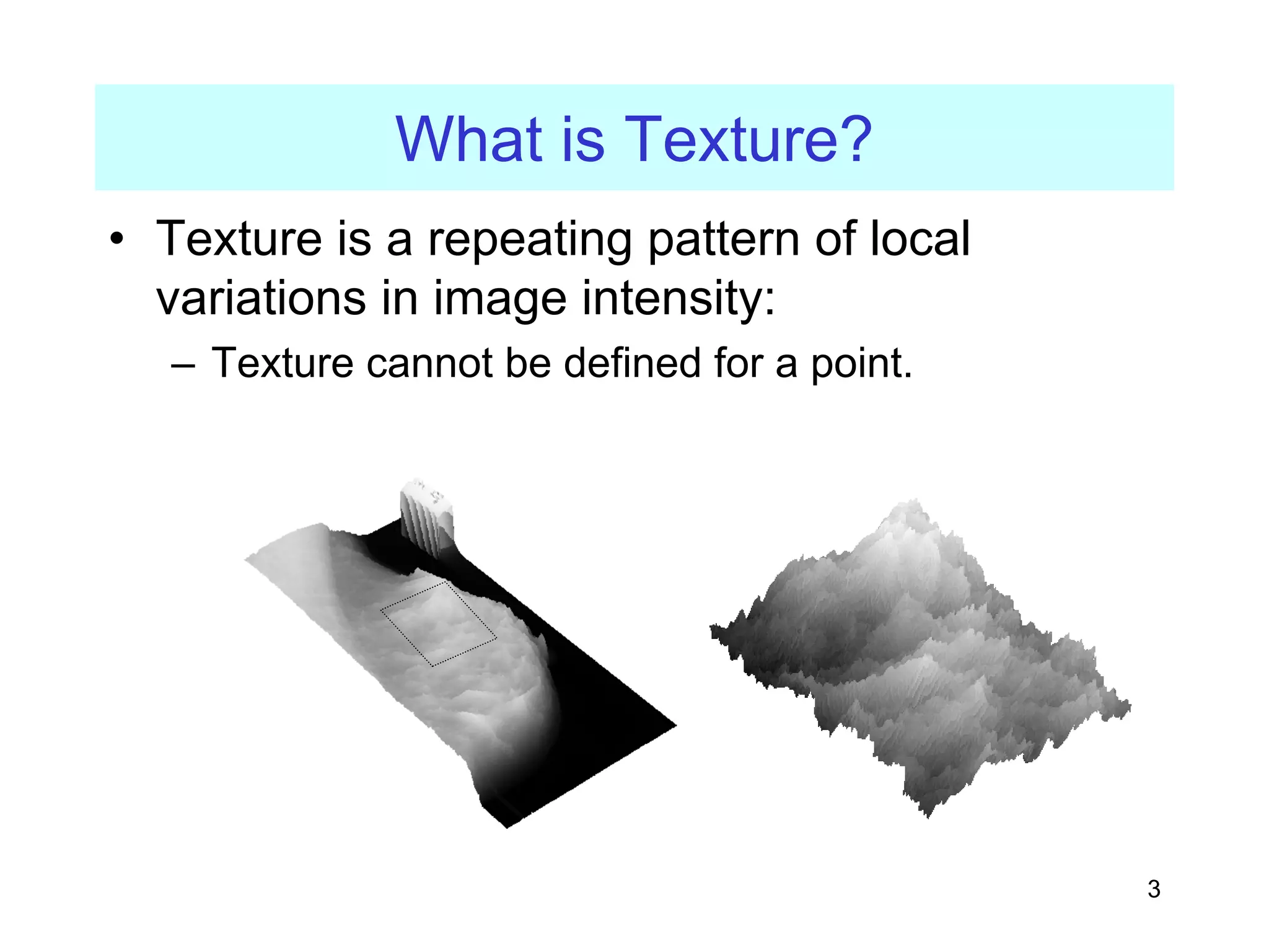
What is Texture?
• Texture is a repeating pattern of local
variations in image intensity:
– Texture cannot be defined for a point.

4. 4
What is Texture?
• For example, an image has a 50% black and
50% white distribution of pixels.
• Three different images with the same
intensity distribution, but with different
textures.

5. 5
Texture
• Texture consists of texture primitives or
texture elements, sometimes called texels.
– Texture can be described as fine, coarse, grained,
smooth, etc.
– Such features are found in the tone and structure
of a texture.
– Tone is based on pixel intensity properties in the
texel, whilst structure represents the spatial
relationship between texels.

6. 6
Texture
– If texels are small and tonal differences between
texels are large a fine texture results.
– If texels are large and consist of several pixels, a
coarse texture results.

7. 7
Texture Analysis
• There are two primary issues in texture
analysis:
n texture classification
o texture segmentation
• Texture segmentation is concerned with
automatically determining the boundaries
between various texture regions in an image.
• Reed, T.R. and J.M.H. Dubuf, CVGIP: Image Understanding, 57: pp.
359-372. 1993.

8. 8
Texture Classification
• Texture classification is concerned with
identifying a given textured region from a
given set of texture classes.
– Each of these regions has unique texture
characteristics.
– Statistical methods are extensively used.
e.g. GLCM, contrast, entropy, homogeneity

9. 9
Defining Texture
• There are three approaches to defining
exactly what texture is:
c Structural: texture is a set of primitive texels in
some regular or repeated relationship.
d Statistical: texture is a quantitative measure of the
arrangement of intensities in a region. This set of
measurements is called a feature vector.
e Modelling: texture modelling techniques involve
constructing models to specify textures.

10. 10
Defining Texture
• Statistical methods are particularly useful
when the texture primitives are small,
resulting in microtextures.
• When the size of the texture primitive is large,
first determine the shape and properties of
the basic primitive and the rules which govern
the placement of these primitives, forming
macrotextures.

11. 11
Simple Analysis of Texture

12. 12
Range
• One of the simplest of the texture
operators is the range or
difference between maximum and
minimum intensity values in a
neighborhood.
– The range operator converts the
original image to one in which
brightness represents texture.

13. 13
Variance
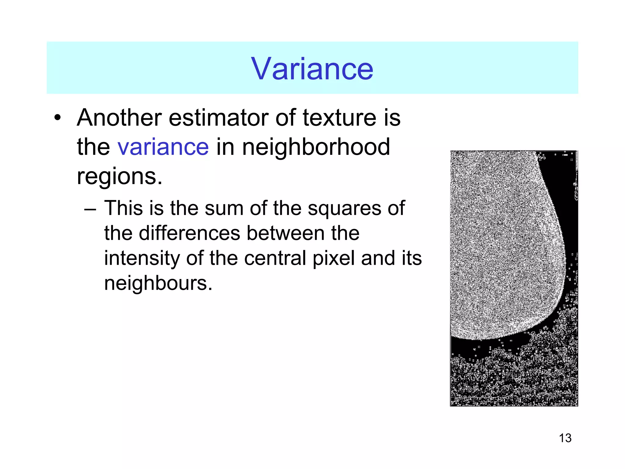
• Another estimator of texture is
the variance in neighborhood
regions.
– This is the sum of the squares of
the differences between the
intensity of the central pixel and its
neighbours.

14. 14
Quantitative Texture Measures
• Numeric quantities or statistics that describe
a texture can be calculated from the
intensities (or colours) themselves

15. 15
Grey Level Co-occurrence
• The statistical measures described so far are
easy to calculate, but do not provide any
information about the repeating nature of
texture.
• A gray level co-occurrence matrix (GLCM)
contains information about the positions of
pixels having similar gray level values.

16. 16
GLCM
• A co-occurrence matrix is a two-dimensional
array, P, in which both the rows and the
columns represent a set of possible image
values.
– A GLCM Pd[i,j] is defined by first specifying a
displacement vector d=(dx,dy) and counting all
pairs of pixels separated by d having gray levels i
and j.
– The GLCM is defined by:
[ , ]
d ij
P i j n
=

17. 17
GLCM
– where nij is the number of occurrences of the pixel
values (i,j) lying at distance d in the image.
– The co-occurrence matrix Pd has dimension n×n,
where n is the number of gray levels in the image.

18. 18
GLCM
• For example, if d=(1,1)
there are 16 pairs of pixels in the image
which satisfy this spatial separation. Since
there are only three gray levels, P[i,j] is a 3×3
matrix.
2 1 2 0 1
0 2 1 1 2
0 1 2 2 0
1 2 2 0 1
2 0 1 0 1
i
j
0 2 2
2 1 2
2 3 2
d
P =
0
1 i
2
0 1 2
j

19. 19
GLCM
Algorithm:
• Count all pairs of pixels in which the first pixel
has a value i, and its matching pair displaced
from the first pixel by d has a value of j.
• This count is entered in the ith row and jth
column of the matrix Pd[i,j]
• Note that Pd[i,j] is not symmetric, since the
number of pairs of pixels having gray levels
[i,j] does not necessarily equal the number of
pixel pairs having gray levels [j,i].

20. 20
Normalised GLCM
• The elements of Pd[i,j] can be normalised by
dividing each entry by the total number of
pixel pairs.
Normalised GLCM; N[i,j], defined by:
which normalises the co-occurrence values to
lie between 0 and 1, and allows them to be
thought of as probabilities.
[ , ]
[ , ]
[ , ]
i j
P i j
N i j
P i j
=
∑∑

21. 21
Numeric Features of GLCM
• Gray level co-occurrence matrices capture
properties of a texture but they are not
directly useful for further analysis, such as the
comparison of two textures.
• Numeric features are computed from the co-
occurrence matrix that can be used to
represent the texture more compactly.

22. 22
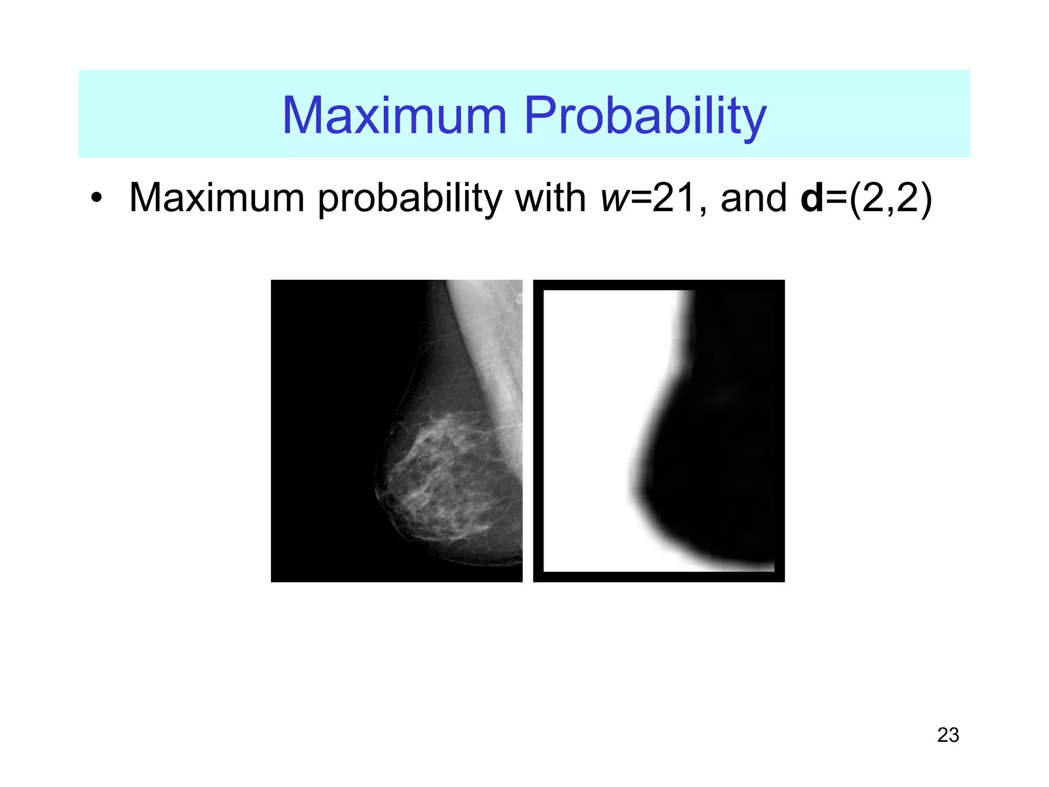
Maximum Probability
• This is simply the largest entry in the matrix,
and corresponds to the strongest response.
– This could be the maximum in any of the matrices
or the maximum overall.
,
max [ , ]
m d
i j
C P i j
=

23. 23
Maximum Probability
• Maximum probability with w=21, and d=(2,2)

24. 24
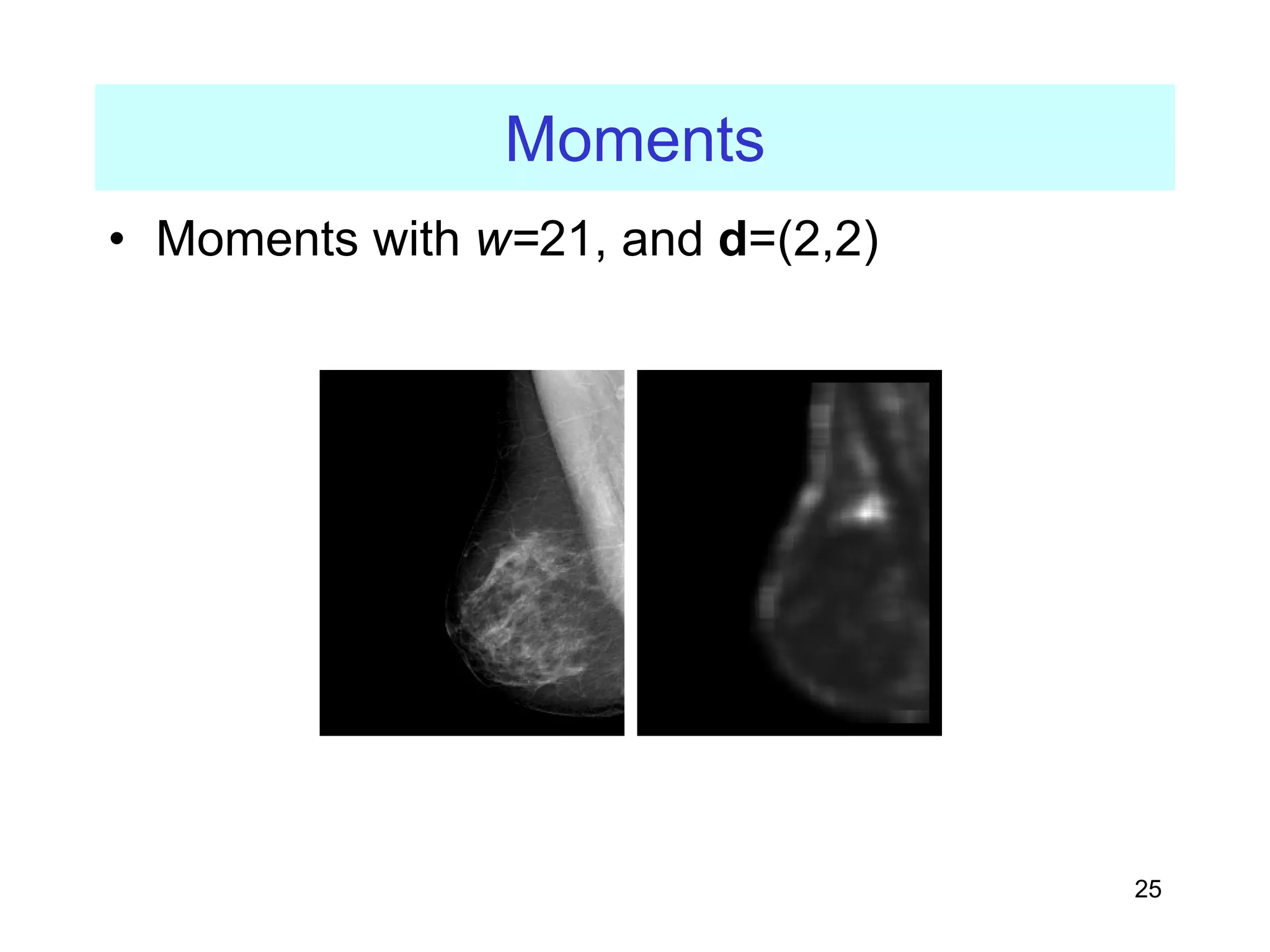
Moments
• The order k element difference moment can
be defined as:
• This descriptor has small values in cases
where the largest elements in P are along the
principal diagonal. The opposite effect can be
achieved using the inverse moment.
( ) [ , ]
k
k d
i j
Mom i j P i j
= −
∑∑
[ , ]
,
( )
d
k k
i j
P i j
Mom i j
i j
= ≠
−
∑∑

25. 25
Moments
• Moments with w=21, and d=(2,2)

26. 26
Contrast
• Contrast is a measure of the local variations
present in an image.
– If there is a large amount of variation in an image
the P[i,j]’s will be concentrated away from the
main diagonal and contrast will be high.
– (typically k=2, n=1)
( , ) ( ) [ , ]
n
k
d
i j
C k n i j P i j
= −
∑∑

27. 27
Contrast
• Contrast with w=21, and d=(2,2)

28. 28
Homogeneity
• A homogeneous image will result in a co-
occurrence matrix with a combination of high
and low P[i,j]’s.
– Where the range of graylevels is small the P[i,j]
will tend to be clustered around the main diagonal.
– A heterogeneous image will result in an even
spread of P[i,j]’s.
[ , ]
1
d
h
i j
P i j
C
i j
=
+ −
∑∑

29. 29
Homogeneity
• Homogeneity with w=21, and d=(2,2)

30. 30
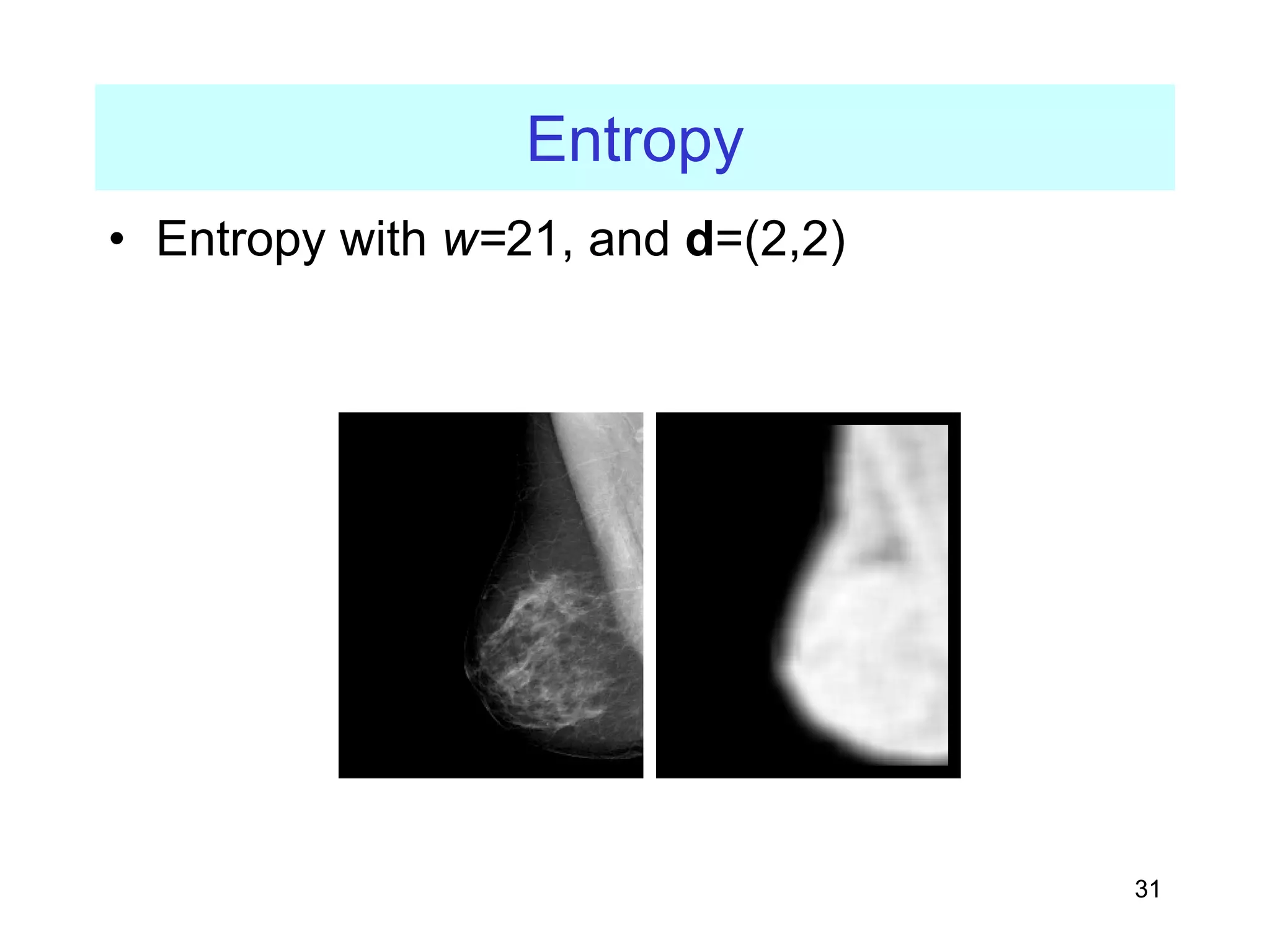
Entropy
• Entropy is a measure of information content.
It measures the randomness of intensity
distribution.
– Such a matrix corresponds to an image in which
there are no preferred graylevel pairs for the
distance vector d.
– Entropy is highest when all entries in P[i,j] are of
similar magnitude, and small when the entries in
P[i,j] are unequal.
[ , ]ln [ , ]
e d d
i j
C P i j P i j
= −∑∑

31. 31
Entropy
• Entropy with w=21, and d=(2,2)

32. 32
Correlation
• Correlation is a measure of image linearity
• Correlation will be high if an image contains a
considerable amount of linear structure.
[ ]
[ , ]
d i j
i j
c
i j
ijP i j
C
µ µ
σ σ
−
=
∑∑
2 2 2
[ , ], [ , ]
i d i d i
iP i j i P i j
µ σ µ
= = −
∑ ∑

33. 33
GLCM - References
• Carlson, G.E. and W.J. Ebel. "Co-occurrence matrix modification for
small region texture measurement and comparison". in IGARSS'88-
Remote Sensing: Moving Towards the 21st Century, pp.519-520, IEEE,
Edinburgh, Scotland. 1988.
• Argenti, F., L. Alparone, and G. Benelli, "Fast algorithms for texture
analysis using co-occurrence matrices". IEE Proceedings, Part F:
Radar and SIgnal Processing, 137(6): pp. 443-448. 1990.
• Gotlieb, C.C. and H.E. Kreyszig, "textur descriptors based on co-
occurrence matrices". Computer Vision, Graphics and Image
Processing, 51(1): pp. 70-86. 1990.

34. 34
Problems with GLCM
• One problem with deriving texture
measures from co-occurrence matrices
is how to choose the displacement
vector d.
– The choice of the displacement vector is an important parameter in the
definition of the GLCM.
– Occasionally the GLCM is computed from several values of d and the one
which maximises a statistical measure computed from P[i,j] is used.
– Zucker and Terzopoulos used a χ2 measure to select the values of d that
have the most structure; i.e. to maximise the value:
2
2 [ , ]
( ) 1
[ ] [ ]
d
i j d d
P i j
d
P i P j
χ = −
∑∑

35. 35
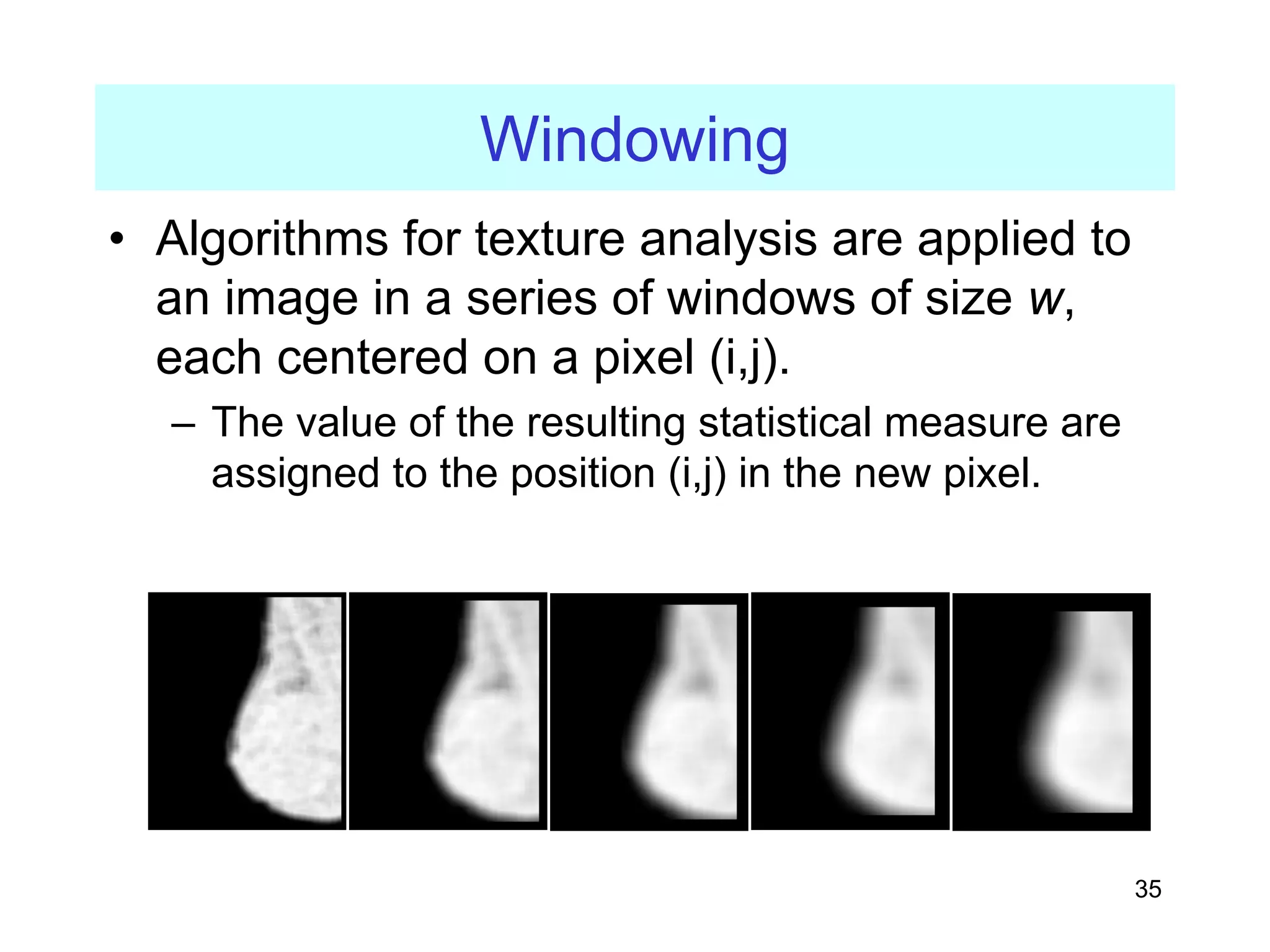
Windowing
• Algorithms for texture analysis are applied to
an image in a series of windows of size w,
each centered on a pixel (i,j).
– The value of the resulting statistical measure are
assigned to the position (i,j) in the new pixel.

36. 36
Haralick Texture Operator
• Haralick et al. suggested a set of 14 textural
features which can be extracted from the co-
occurrence matrix, and which contain
information about image textural
characteristics such as homogeneity,
linearity, and contrast.
• Haralick, R.M., K. Shanmugam, and I. Dinstein, "Textural features for
image classification". IEEE Transactions on Systems, Man and
Cybernetics: pp. 610-621. 1973.

37. 37
Graylevel Difference Statistics
• Grey-level differences are based on absoute
differences between pairs of grey-levels.
• The grey-level differences are contained in a
256-element vector, and are computed by
taking the absolute differences of all possible
pairs of grey levels distance d apart at angle
θ, and counting the number of times the
difference is 0,1,…,255

38. 38
Graylevel Difference Statistics
• Let d=(dx,dy) be the displacement vector
between two image pixels, and g(d) the gray-
level difference at distance d.
• pg(g,d) is the histogram of the gray-level
differences at the specific distance, d. One
distinct histogram exists for each distance d.
( ) ( , ) ( , )
g d f i j f i dx j dy
= − + +

39. 39
Graylevel Difference Statistics
• The difference statistics are then normalized
by dividing each element of the vector by the
number of possible pixel pairs.
• Several texture measures can be extracted
from the histogram of graylevel differences:

40. 40
Graylevel Difference Statistics
• Mean:
– Small mean values µd indicate coarse texture
having a grain size equal to or larger than the
magnitude of the displacement vector.
• Entropy:
– This is a measure of the homogeneity of the
histogram. It is maximised for uniform histograms.
1
( , )
N
d k g k
k
g p g d
µ
=
= ∑
1
( , )ln ( , )
N
d g k g k
k
H p g d p g d
=
= −∑

41. 41
Graylevel Difference Statistics
• Variance:
– The variance is a measure of the dispersion of the
gray-level differences at a certain distance, d.
• Contrast:
2 2
1
( ) ( , )
N
d k d g k
k
g p g d
σ µ
=
= −
∑
2
1
( , )
N
d k g k
k
C g p g d
=
= ∑

42. 42
Graylevel Difference Statistics
Mean Standard Deviation Entropy Contrast

43. 43
Runlength Statistics
• The lengths of texture primitives in different
directions can serve as a texture description.
– A run length is a set of constant intensity pixels
located in a line.
• Runlength statistics are calculated by
counting the number of runs of a given length
(from 1 to n) for each grey level.
• Galloway, M.M., "Texture classification using gray level run lengths".
Computer Graphics and Image Processing, 4(2): pp. 172-179. 1975.

44. 44
Runlength Statistics
• In a course texture it is expected that long
runs will occur relatively often, whereas a fine
texture will contain a higher proportion of
short runs.
• Statistical measures:
– Let B(a,r) be the number of primitives of all
directions having length r, and grey-level a, m and
n the image dimensions, and L the number of
intensity values.
– Let K be the number of runs: 1 1
( , )
L Nr
a r
K B a r
= =
= ∑∑

45. 45
Runlength Statistics
c Long-run emphasis:
– This is a measure that emphasizes the long-runs of a gray-
level image. Long-run emphasis will be large when there are
lots of long runs of the same intensity.
d Short-run emphasis:
– This is a measure that emphasizes the short-runs of a gray-
level image. short-run emphasis will be large when
there are lots of short runs of the same intensity.
2
1
1 1
( , )
L Nr
lr K
a r
S B a r r
= =
= ∑∑
1
2
1 1
( , )
L Nr
sr K
a r
B a r
S
r
= =
= ∑∑

46. 46
Runlength Statistics
e Grey-level distribution:
– The sum in [ ] gives the total number of runs for a certain
gray-level value grey-level a. The distribution will be large
when runs are not evenly distributed over the different
intensities.
2
2
1
1 1
( , )
L Nr
d K
a r
S B a r r
= =
 
=  
 
∑ ∑

47. 47
Runlength Statistics
f Run-length distribution:
– The sum in [ ] gives the total number of occurrences of a
certain run length l for any gray level. s for a certain gray-
level value grey-level r.
g Run percentage:
rp
K
S
mn
=
2
2
1
1 1
( , )
Nr L
rd K
r a
S B a r r
= =
 
=  
 
∑ ∑

48. 48
Edges and Texture
• It should be possible to locate the edges that result
from the intensity transitions along the boundary of
the texture.
– Since a texture will have large numbers of texels, there
should be a property of the edge pixels that can be used to
characterise the texture.
• a set of common directions
• a measure of the locadensity of the edge pixels
• Compute the co-occurrence matrix of an edge-
enhanced image.
• Davis, L.S. and A. Mitiche, "Edge detection in textures". Computer
Graphics and Image Processing, 12: pp. 25-39. 1980.

49. 49
Edges and Texture
Original Sobel-Enhanced Contrast

50. 50
Energy and Texture
• One approach to generating texture features
is to use local kernels to detect various types
of texture.
• Laws† developed a texture-energy approach
that measures the amount of variation within
a fixed-size window.
• † Laws, K.I. "Rapid texture identification". in SPIE Image Processing for
Missile Guidance, pp.376-380. 1980.

51. 51
Laws
• A set of convolution kernels are used to
compute texture energy.
• The kernels are computed from the following
vectors:
[ ]
[ ]
[ ]
[ ]
[ ]
L5 1 4 6 4 1
E5 1 2 0 2 1
S5 1 0 2 0 1
R5 1 4 6 4 1
W5 1 2 0 2 1
=
= − −
= − −
= − −
= − − −

52. 52
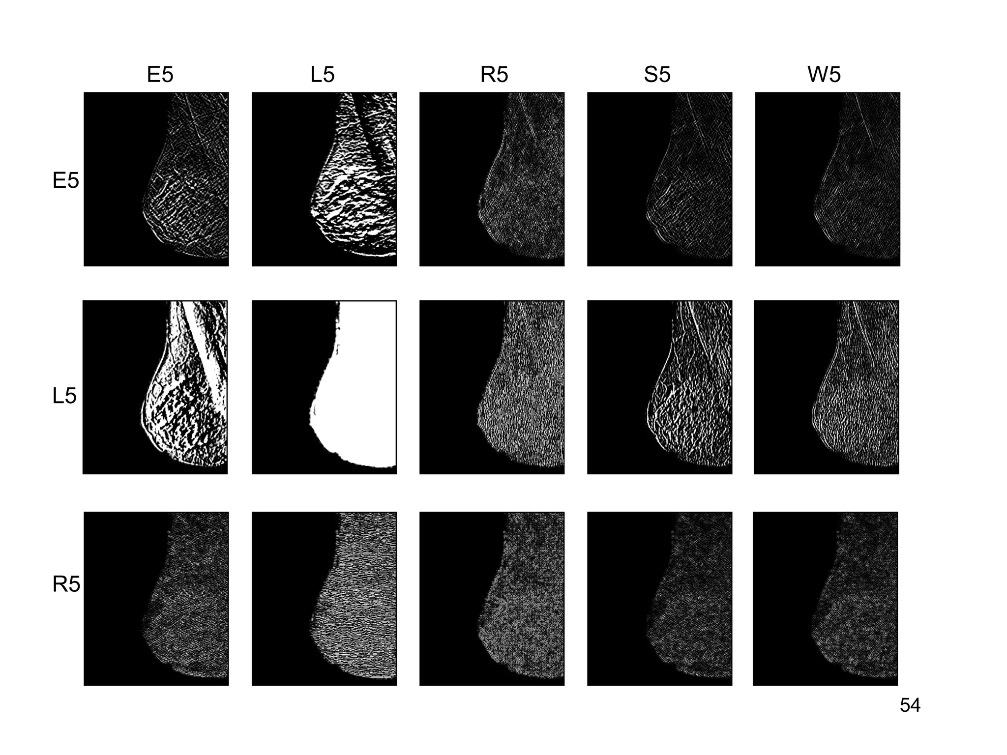
Laws
• The L5 (level) vector gives a centre-weighted
local average. The E5 (edge) vector detects
edges, the S5 (spot) vector detects spots, the
R5 (ripple) vector detects ripples, and the W5
(wave) vector detects waves.
• The two-dimensional convolution kernels are
obtained by computing the outer product of a
pair of vectors.

53. 53
Laws
e.g. E5L5 is computed as the product of E5
and L5 as follows:
• This results in 25 5×5 kernels, 24 of the
kernels are zero-sum, the L5L5 is not.
[ ]
1 1 4 6 4 1
2 2 8 12 8 2
1 4 6 4 1
0 0 0 0 0 0
2 2 8 12 8 2
1 1 4 6 4 1
− − − − − −
   
   
− − − − − −
   
   
× =
   
   
   
   

54. 54
E5 L5 R5 S5 W5
E5
L5
R5

55. 55
E5 L5 R5 S5 W5
S5
W5

56. 56
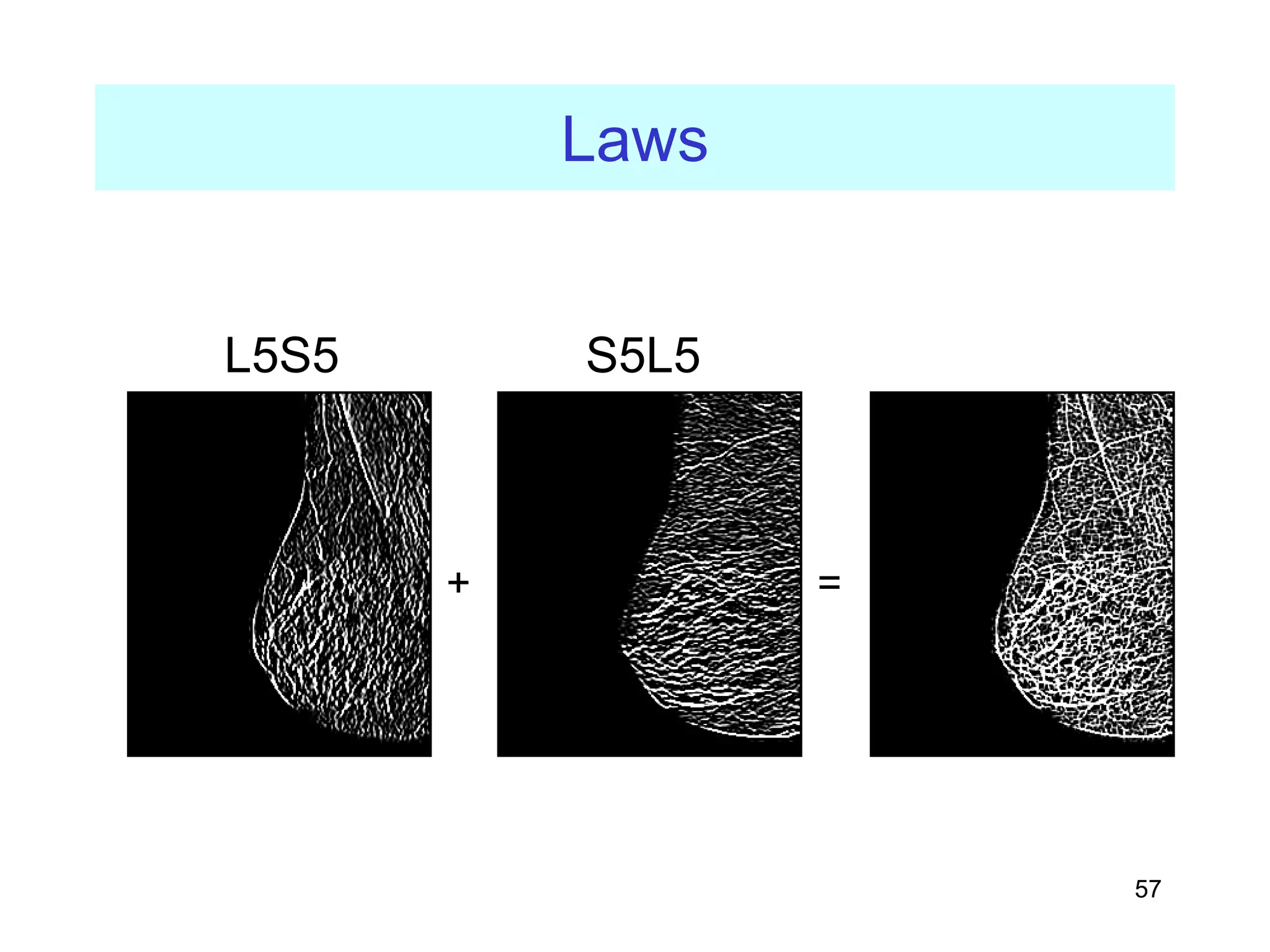
Laws
• Bias from the “directionality” of textures can
be removed by combining symmetric pairs of
features, making them rotationally invariant.
e.g. S5L5(H) + L5S5(V) = L5S5R

57. 57
Laws
L5S5 S5L5
+ =

58. 58
Laws
• After the colvolution with the specified kernel,
the texture energy measure (TEM) is
computed by summing the absolute values in
a local neghborhood:
• If n kernels are applied, the result is an n-
dimensional feature vector at each pixel of
the image being analysed.
1 1
( , )
m n
e
i j
L C i j
= =
= ∑∑

59. 59
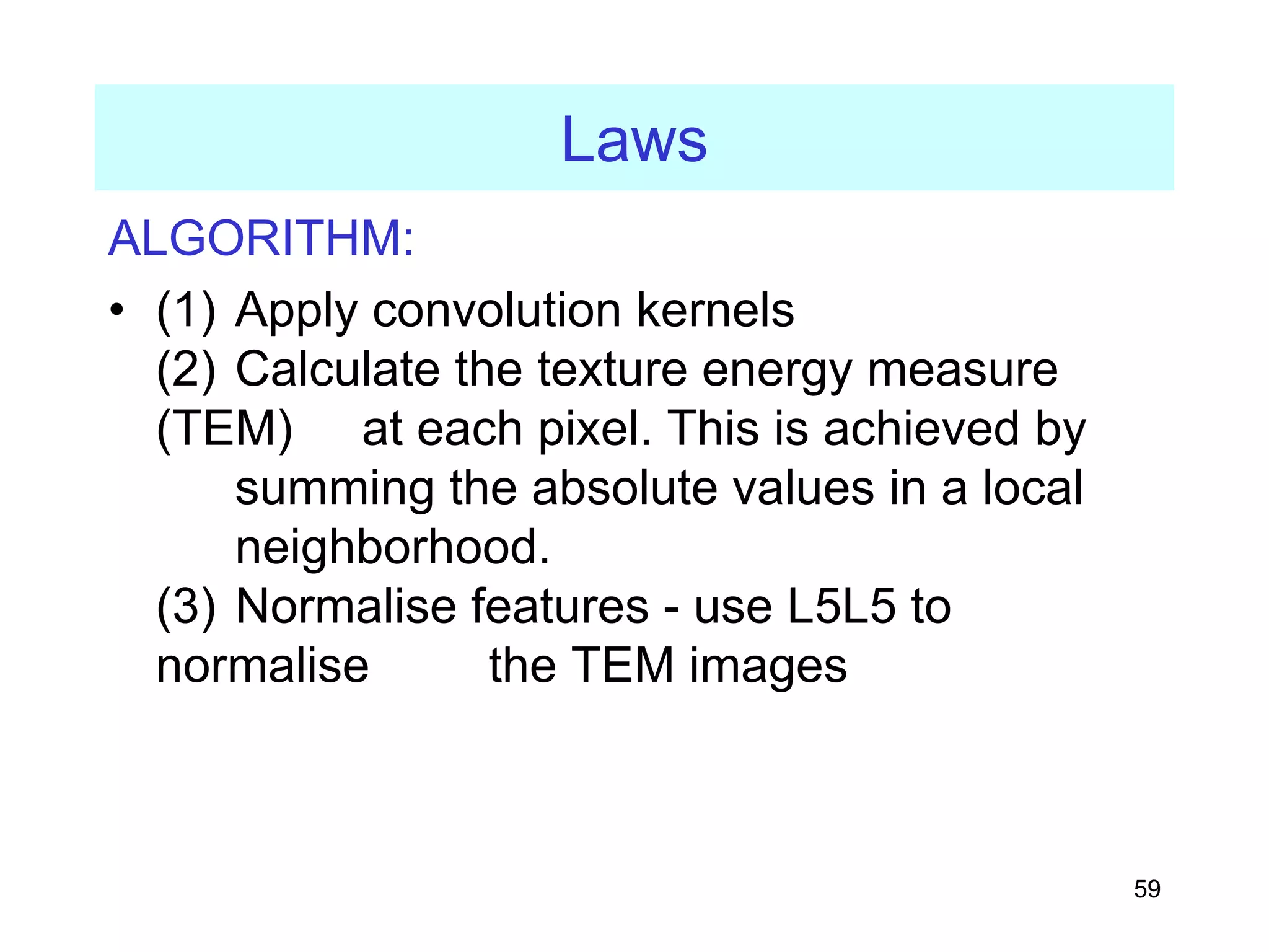
Laws
ALGORITHM:
• (1) Apply convolution kernels
(2) Calculate the texture energy measure
(TEM) at each pixel. This is achieved by
summing the absolute values in a local
neighborhood.
(3) Normalise features - use L5L5 to
normalise the TEM images

60. 60
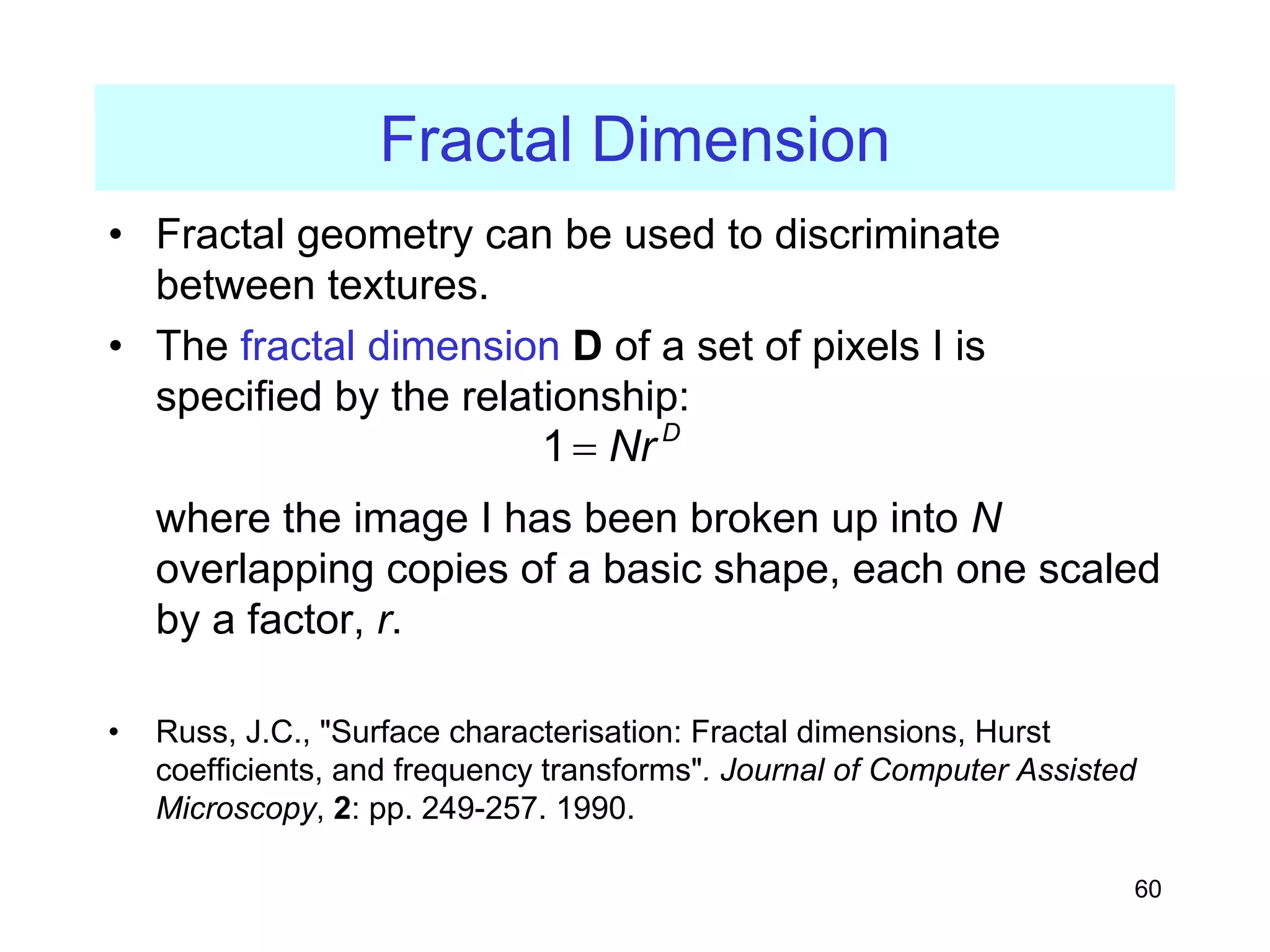
Fractal Dimension
• Fractal geometry can be used to discriminate
between textures.
• The fractal dimension D of a set of pixels I is
specified by the relationship:
where the image I has been broken up into N
overlapping copies of a basic shape, each one scaled
by a factor, r.
• Russ, J.C., "Surface characterisation: Fractal dimensions, Hurst
coefficients, and frequency transforms". Journal of Computer Assisted
Microscopy, 2: pp. 249-257. 1990.
1 D
Nr
=

61. 61
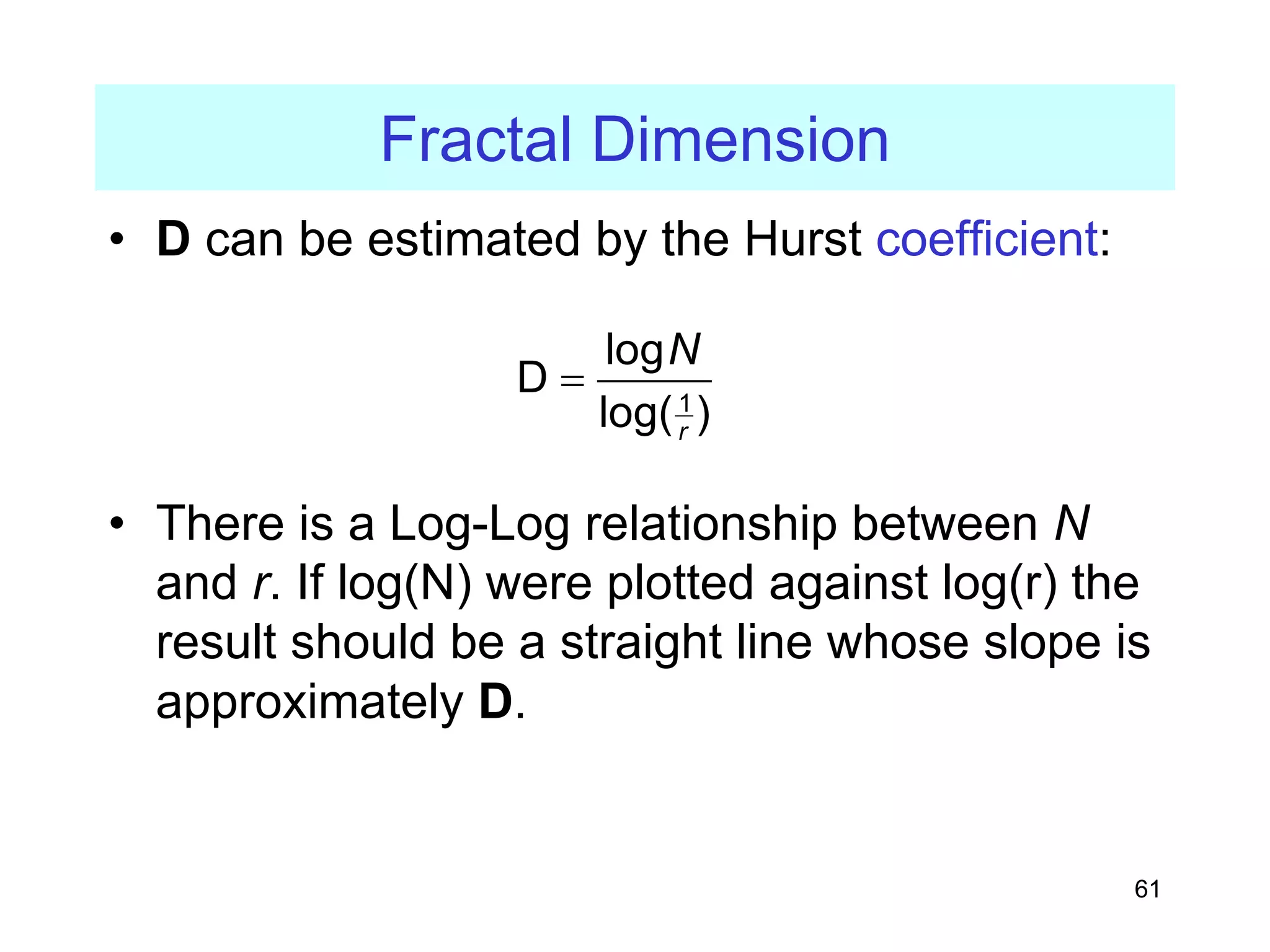
Fractal Dimension
• D can be estimated by the Hurst coefficient:
• There is a Log-Log relationship between N
and r. If log(N) were plotted against log(r) the
result should be a straight line whose slope is
approximately D.
1
log
D
log( )
r
N
=

62. 62
Hurst
• The Hurst-coefficient is an approximation that
makes use of this relationship.
– Consider a 7×7 pixel region which is marked according to
the distance of each pixel from the central pixel.
– There are eight groups of pixels, corresponding to the eight
difference distances that are possible
Central pixel (d=0)
Distance = 1
Distance = sqrt(2)
Distance = 2
Distance = sqrt(5)
Distance = sqrt(8)
Distance = 3
Distance = sqrt(10)

63. 63
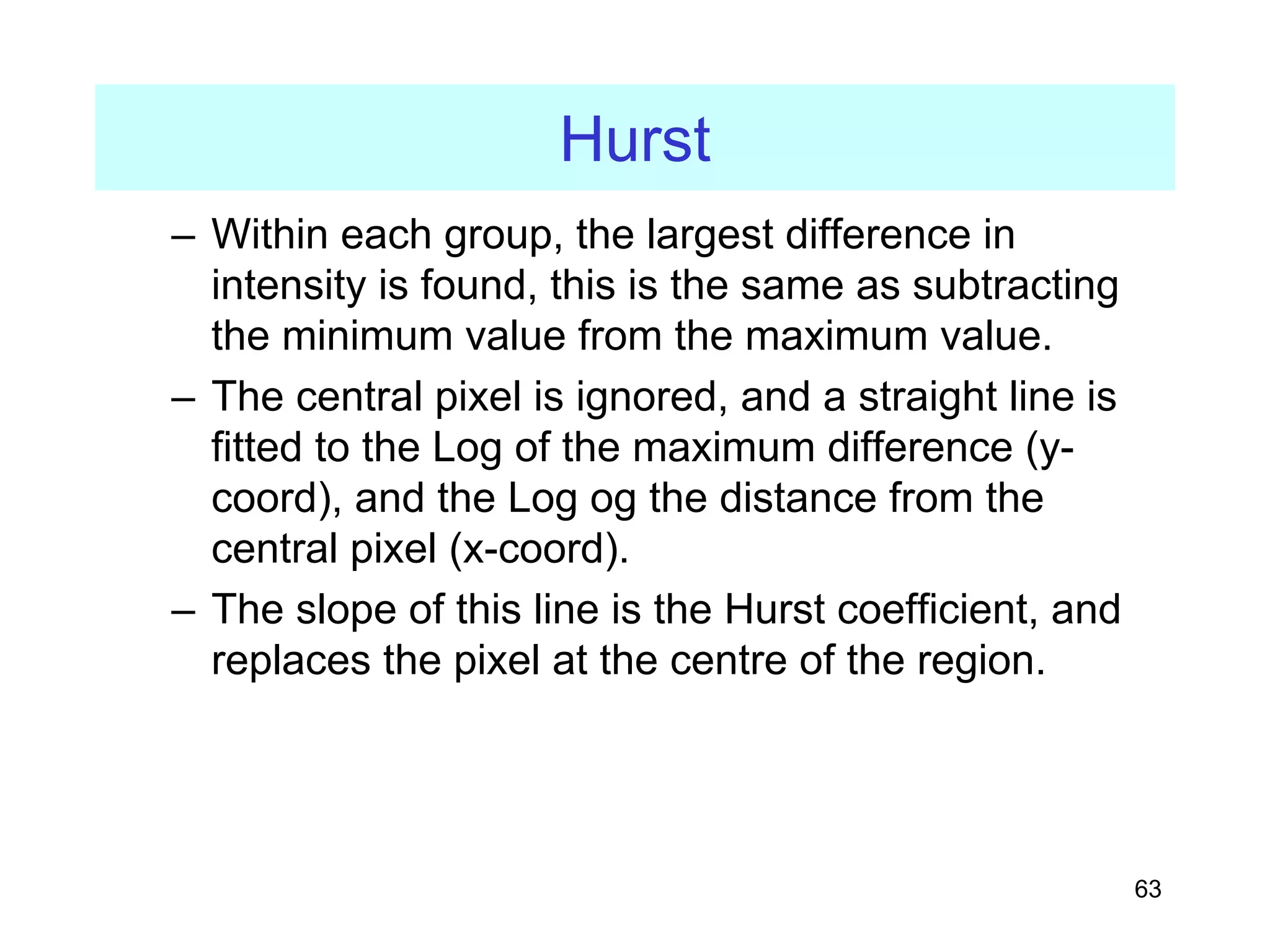
Hurst
– Within each group, the largest difference in
intensity is found, this is the same as subtracting
the minimum value from the maximum value.
– The central pixel is ignored, and a straight line is
fitted to the Log of the maximum difference (y-
coord), and the Log og the distance from the
central pixel (x-coord).
– The slope of this line is the Hurst coefficient, and
replaces the pixel at the centre of the region.

64. 64
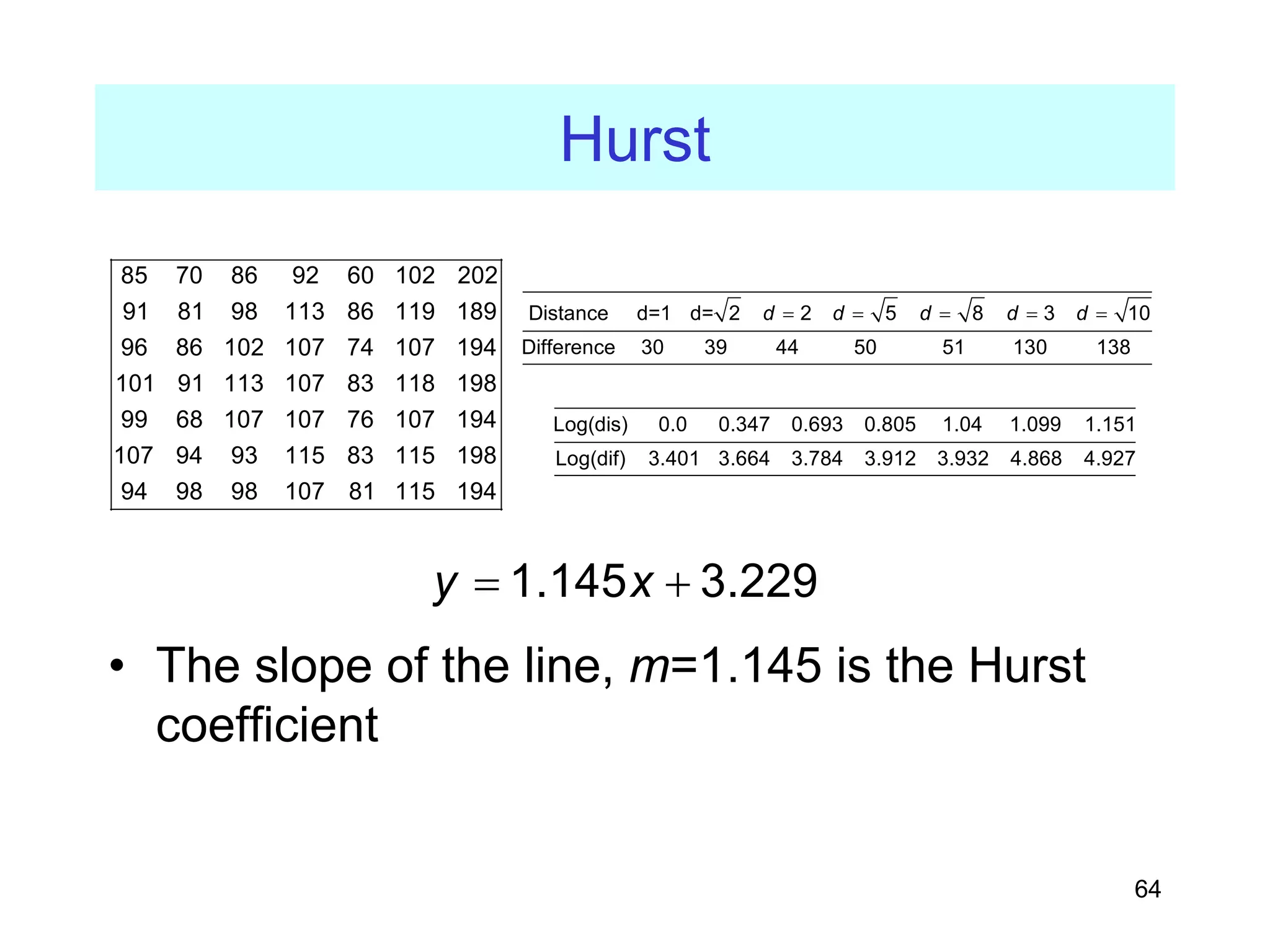
Hurst
• The slope of the line, m=1.145 is the Hurst
coefficient
85 70 86 92 60 102 202
91 81 98 113 86 119 189
96 86 102 107 74 107 194
101 91 113 107 83 118 198
99 68 107 107 76 107 194
107 94 93 115 83 115 198
94 98 98 107 81 115 194
Distance d=1 d= 2 2 5 8 3 10
Difference 30 39 44 50 51 130 138
d d d d d
= = = = =
Log(dis) 0.0 0.347 0.693 0.805 1.04 1.099 1.151
Log(dif) 3.401 3.664 3.784 3.912 3.932 4.868 4.927
1.145 3.229
y x
= +

65. 65
Hurst

66. 66
Surfaces and Texture
• There are some algorithms that are based on
a view of the gray-level image as a three-
dimensional surface, where intensity is the
third dimension.
– Vector dispersion
• Matalas, I., S. Roberts, and H. Hatzakis. "A set of
multiresolution texture features suitable for unsupervised
image segmentation". in SIgnal Processing VIII: Theories
and Applications. 1996.
– Surface curvature
• Peet, F.G. and T.S. Sahota, "Surface curvature as a measure
of image texture". IEEE Transactions on Pattern Analysis and
Machine Intelligence, 7(6): pp. 734-738. 1985.

67. 67
Model-based Methods
• Model-based methods for texture analysis is
an approach used to characterize texture
which determines an analytical model of the
textured image being analyzed.
– Such models have a set of parameters.
– The values of these parameters determine the
properties of the texture, which may be
synthesized by applying the model.
e.g. Markov random fields

68. 68
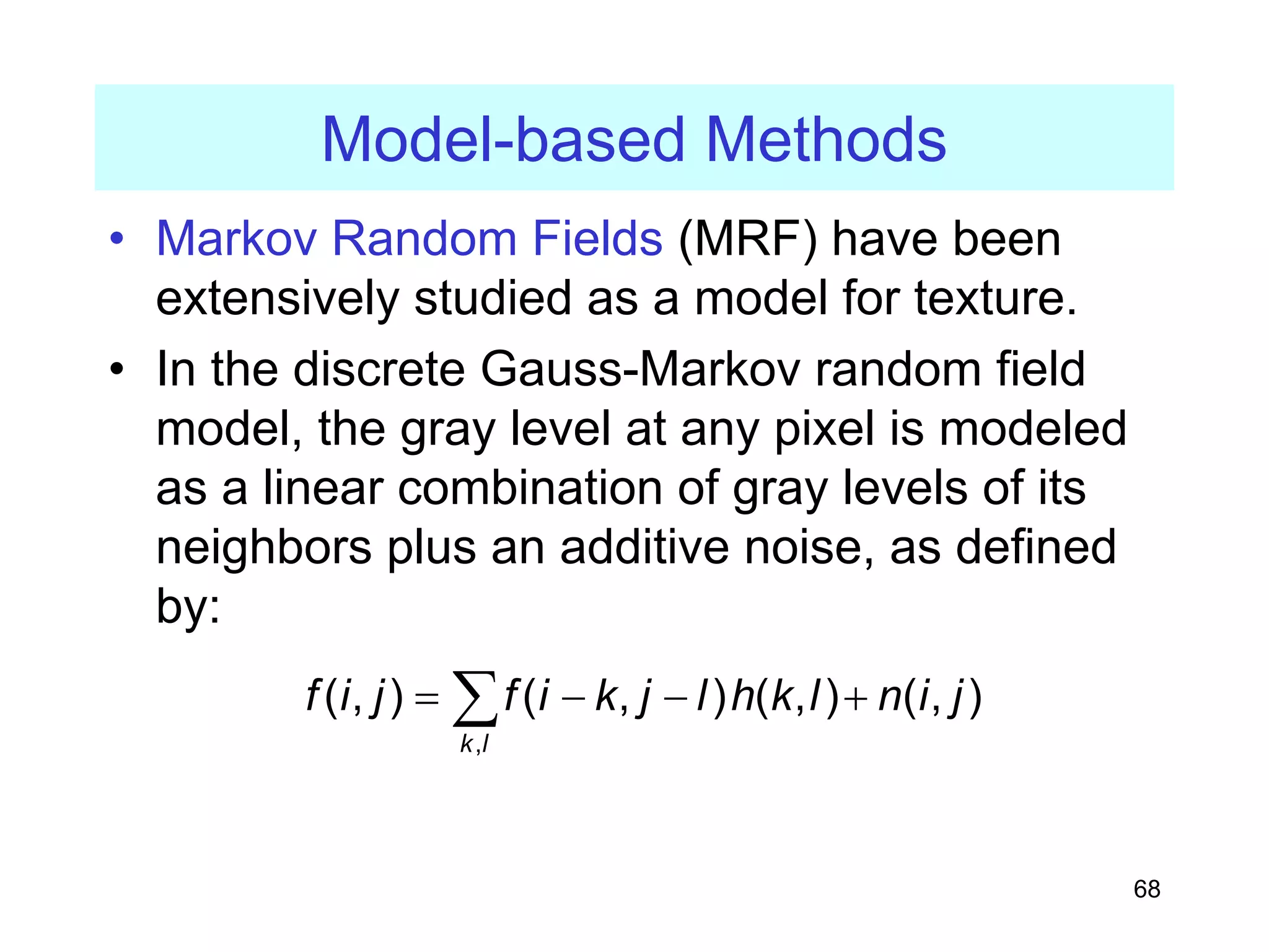
Model-based Methods
• Markov Random Fields (MRF) have been
extensively studied as a model for texture.
• In the discrete Gauss-Markov random field
model, the gray level at any pixel is modeled
as a linear combination of gray levels of its
neighbors plus an additive noise, as defined
by:
,
( , ) ( , ) ( , ) ( , )
k l
f i j f i k j l h k l n i j
= − − +
∑

69. 69
Model-based Methods
– The summation is carried out over a specified set
of pixels which are neighbors to the pixel (i,j)
– The parameters of this model are the weights
h(k,l).
– These parameters are computed from the given
texture using least-squares method.
– These estimated parameters are then compared
with those of the known texture class to determine
the class of the particular texture being analysed.

70. 70
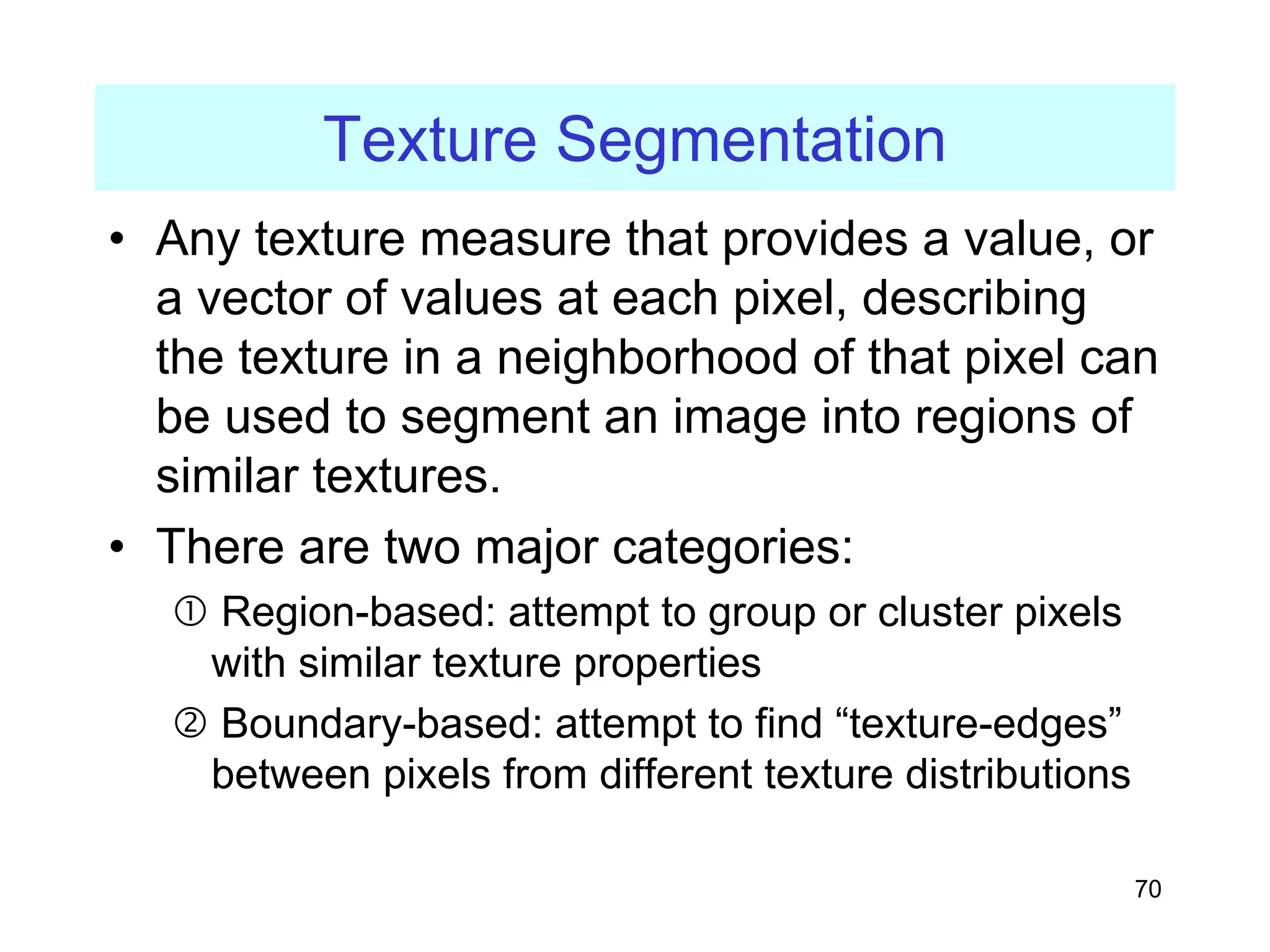
Texture Segmentation
• Any texture measure that provides a value, or
a vector of values at each pixel, describing
the texture in a neighborhood of that pixel can
be used to segment an image into regions of
similar textures.
• There are two major categories:
c Region-based: attempt to group or cluster pixels
with similar texture properties
d Boundary-based: attempt to find “texture-edges”
between pixels from different texture distributions

71. 71
Texture Segmentation
GLC: Entropy Original T=4 Entropy T=12 Breast Contour
(Wsize =13) Approximation