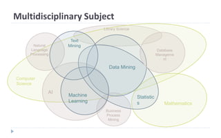
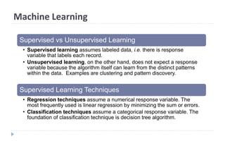
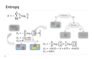
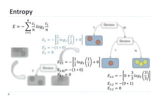
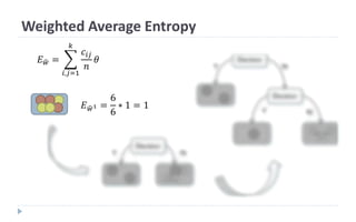
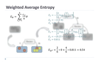
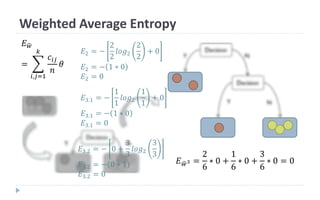
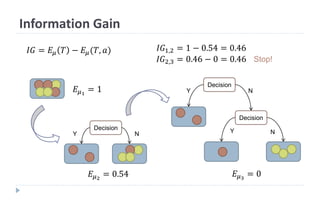
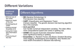
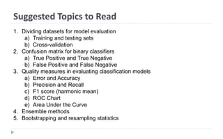
Decision Tree Learning
Supervised Learning
Adrian Cuyugan
Information Analytics
Multidisciplinary Subject
Statistic
s
Data Mining
Machine
Learning
AI
Text
Mining
Business
Process
Mining
Natural
Language
Processing
Database
Manageme
nt
Library Science
Mathematics
Computer
Science
Machine Learning
Supervised vs Unsupervised Learning
• Supervised learning assumes labeled data, i.e. there is response
variable that labels each record.
• Unsupervised learning, on the other hand, does not expect a response
variable because the algorithm itself can learn from the distinct patterns
within the data. Examples are clustering and pattern discovery.
Supervised Learning Techniques
• Regression techniques assume a numerical response variable. The
most frequently used is linear regression by minimizing the sum or errors.
• Classification techniques assume a categorical response variable. The
foundation of classification technique is decision tree algorithm.
Entropy
In other words, the algorithm splits the set
of instances in subsets such that the
variation within each subset becomes
smaller.
Entropy is an information-theoritic
measure for the uncertainly in a
multi-set of elements.
If the multi-set contains many
different elements and each element
is unique, then variation is maximal
and it takes many bits to encode the
individual elements. Hence, the
entropy is considered high.
If all elements, on the other hand,
are the same, then actually no bits
are needed to encode the individual
elements, hence it is a low entropy.
Decision
Y N
Entropy
Decision
Y N
Decision
Y N
Decision
High Entropy
High EntropyLow Entropy
Low Entropy
Low Entropy Low Entropy
Y N
Entropy
𝐸 = −
𝑖=1
𝑘
𝑐𝑖
𝑛
𝑙𝑜𝑔2
𝑐𝑖
𝑛
𝐸1 = −
3
6
𝑙𝑜𝑔2
3
6
+
3
6
𝑙𝑜𝑔2
3
6
𝐸1 = − 0.5 ∗ −1 + 0.5 ∗ −1
𝐸1 = 1
Entropy
𝐸 = −
𝑖=1
𝑘
𝑐𝑖
𝑛
𝑙𝑜𝑔2
𝑐𝑖
𝑛
𝐸2 = −
2
2
𝑙𝑜𝑔2
2
2
+ 0
𝐸2 = − 1 ∗ 0
𝐸2 = 0
𝐸3 = −
1
4
𝑙𝑜𝑔2
1
4
+
3
4
𝑙𝑜𝑔2
3
4
𝐸3 = − 0.25 ∗ −2 + 0.75 ∗ −0.415
𝐸3 = 0.811
Entropy
𝐸 = −
𝑖=1
𝑘
𝑐𝑖
𝑛
𝑙𝑜𝑔2
𝑐𝑖
𝑛
𝐸2 = −
2
2
𝑙𝑜𝑔2
2
2
+ 0
𝐸2 = − 1 ∗ 0
𝐸2 = 0
𝐸3.1 = −
1
1
𝑙𝑜𝑔2
1
1
+ 0
𝐸3.1 = − 1 ∗ 0
𝐸3.1 = 0 𝐸3.2 = − 0 +
3
3
𝑙𝑜𝑔2
3
3
𝐸3.2 = − 0 ∗ 1
𝐸3.2 = 0
Weighted Average Entropy
𝐸 𝑤1 =
6
6
∗ 1 = 1
𝐸 𝑤 =
𝑖,𝑗=1
𝑘
𝑐𝑖𝑗
𝑛
𝜃
Weighted Average Entropy
𝐸2 = −
2
2
𝑙𝑜𝑔2
2
2
+ 0
𝐸2 = − 1 ∗ 0
𝐸2 = 0
𝐸3 = −
1
4
𝑙𝑜𝑔2
1
4
+
3
4
𝑙𝑜𝑔2
3
4
𝐸3 = − 0.25 ∗ −2 + 0.75 ∗ −0.415
𝐸3 = 0.811
𝐸 𝑤2 =
2
6
∗ 0 +
4
6
∗ 0.811 = 0.54
𝐸 𝑤 =
𝑖,𝑗=1
𝑘
𝑐𝑖𝑗
𝑛
𝜃
Weighted Average Entropy
𝐸2 = −
2
2
𝑙𝑜𝑔2
2
2
+ 0
𝐸2 = − 1 ∗ 0
𝐸2 = 0
𝐸3.1 = −
1
1
𝑙𝑜𝑔2
1
1
+ 0
𝐸3.1 = − 1 ∗ 0
𝐸3.1 = 0
𝐸3.2 = − 0 +
3
3
𝑙𝑜𝑔2
3
3
𝐸3.2 = − 0 ∗ 1
𝐸3.2 = 0
𝐸 𝑤3 =
2
6
∗ 0 +
1
6
∗ 0 +
3
6
∗ 0 = 0
𝐸 𝑤
=
𝑖,𝑗=1
𝑘
𝑐𝑖𝑗
𝑛
𝜃
Information Gain
Decision
Y N
Decision
Y N
Decision
Y N
𝐸𝜇1
= 1
𝐼𝐺 = 𝐸𝜇 𝑇 − 𝐸𝜇(𝑇, 𝑎)
𝐸𝜇2
= 0.54 𝐸𝜇3
= 0
𝐼𝐺1,2 = 1 − 0.54 = 0.46
𝐼𝐺2,3 = 0.46 − 0 = 0.46 Stop!
Different Variations
Additional
Settings
• Minimal size of
the nodes
• Maximum depth
of the tree
• Bootstrapping at
nodes
• Setting minimal
threshold of IG
• Using Gini Index
than Information
Gain
• Post-pruning of
the tree
Different Algorithms
• ID3 (Iterative Dichotomiser 3)
First decision tree classifier.
• CART (Classification and Regression Trees)
A binary classifier. The generic decision tree learning algorithm
like in the example.
• C4.5 and C5.0
Can handle numerical independent variables. The latter offers
more computational speed and varies in splitting rule.
• CHAID (Chi-square Automatic Interaction Detector)
Uses significance testing in splitting.
• Ensembles i.e. Random Forest, Ada Boost, Gradient Boosting
Uses bagging, bootstrapping and weighting. Very flexible and
most recent innovations in decision tree learning.
Suggested Topics to Read
1. Dividing datasets for model evaluation
a) Training and testing sets
b) Cross-validation
2. Confusion matrix for binary classifiers
a) True Positive and True Negative
b) False Positive and False Negative
3. Quality measures in evaluating classification models
a) Error and Accuracy
b) Precision and Recall
c) F1 score (harmonic mean)
d) ROC Chart
e) Area Under the Curve
4. Ensemble methods
5. Bootstrapping and resampling statistics
Text Mining and Analytics
Unsupervised Learning
Adrian Cuyugan
Information Analytics
Text Mining Overview
Data Extraction
• File Types and
Sources (Spreadsheet,
Word Documents,
HTML, JSON, API,
etc.)
• Regular expressions
• Data File Systems
(RDBMS, Google File
System, Hadoop,
MapReduce)
Information
Retrieval
• Intro to Natural
Language Analysis
• Vector Space Model –
Bag of Words
• Term Frequency Matrix
• Inverted Document
Frequency Matrix
• TF-IDF Matrix
• Stop words and
Stemming
• Document Length
Normalization (PL2,
Okapi/BM25)
• Evaluation (Average
Precision, Reciprocal
Rank, F-meaure and
nDCG)
• Query Likelihod,
Statistical Language
Probability Unigram
Language Model
• Rocchio Feedback and
KL Divergence
• Recommender
Systems
Pattern Analysis
• Pattern Discovery
Concepts (Frequent,
Closed and Max)
• Association Rules
• Quantitave Measures
(Support, Confidence
and Lift)
• Other measures
• Apriori Algorithm,
ECLAT and FPGrowth
Algorithms
• Multi-level and Multi-
dimensional levels,
Compressed and
Colossal Patterns
• Sequential Patterns
• Graph Patterns
• Topic Modelling for
Text Data
Clustering
• Partitioning,
Hierarchical and
Density based
methods
• Spectral Clustering
• Probabilistic Models
and EM Algorithm
• Evaluating Clustering
Models
• Clustering streaming
data
• Graph Theory
• Social Network
Analysis
Analytics
• Text clustering,
categorization and
summarization
• Topic-based modelling
• Sentiment analysis
• Integration of free-form
text and structured
data
Visualization
• Basic charts and
graphs
• Animating and
interactivity
• Visualizing
relationships
(hierarchies, clusters
and networks)
• Visualizing text
Text Retrieval
Text Mining and Analytics
Natural Language Analysis
The quick brown fox jumped over the lazy dog.
Pragmatic Analysis
article adjective adjective noun verb preposition article adjective noun
Prepositional phraseNoun phrase
Subject Predicate
Lexical Analysis
(part of speech tagging)
Syntactic Analysis
(parsing)
Semantic Analysis fox (f1) dog (d1) jump (f1, d1)
How quick was the fox that it jumped over the dog.
Could the dog escaped the quick fox if it wasn’t lazy?
Why did the fox jump over the dog?
Vector Space Model
Document (d) The quick brown fox jumped over the lazy dog.
Query (q) How many times does “dog” occur in document?
Term frequency (tf)
Count of query in a document.
Example: count(“dog”, d)
Document length |d| How long is the document?
Document frequency
(df)
How often do we see “dog” in the entire collection?
Example: df(“dog”) = p(“dog” | collection)
Simplest VSM Bag of Words
𝑉𝑆𝑀 𝑞, 𝑑 = 𝑞. 𝑑
= 𝑥1 𝑦1 + … + 𝑥 𝑛 𝑦𝑛
=
𝑖=1
𝑛
𝑥1 𝑦1
𝒒 quick fox over dog
𝑑1 … The quick brown …
𝑑2 The quick brown and over cunny fox…
𝑑3 … the fox is brown and quick…
𝑑4 The quick brown fox … fox … over…
𝑑5
The quick fox … the … the … over brown fox ...
fox
How would you order of
ranking of documents based
on
bit-vector term frequency?
𝑥1, 𝑦1 ∈ 0,1
1 = word is present
0 = word is absent
Bit-Vector Term Frequency Matrix
𝒒 quick fox over dog
𝑑1 … The quick brown …
𝑑2 The quick brown and over cunny fox…
𝑑3 … the fox is brown and quick…
𝑑4 The quick brown fox … fox … over…
𝑑5
The quick fox … the … the … over
brown fox … fox
∈ the quick
brow
n
and is cunny fox over dog
q 0 1 0 0 0 0 1 1 1
𝑑1 0 1 0 0 0 0 0 0 0
𝑑2 0 1 0 0 0 0 1 1 0
𝑑3 0 1 0 0 0 0 1 0 0
𝑑4 0 1 0 0 0 0 1 1 0
𝑑5 0 1 0 0 0 0 1 1 0
𝑓 𝑞, 𝑑1 = 0 ∗ 0 + 1 ∗ 1 + 0 ∗ 0 + 0 ∗ 0 + 0 ∗ 0 + 0 ∗ 0 + 0 ∗ 0 + 0 ∗ 0 + 0 ∗ 0 = 1
𝑓 𝑞, 𝑑3 = 0 ∗ 0 + 1 ∗ 1 + 0 ∗ 0 + 0 ∗ 0 + 0 ∗ 0 + 0 ∗ 0 + 1 ∗ 1 + 0 ∗ 0 + 0 ∗ 0 = 2
𝑓 𝑞, 𝑑5 = 0 ∗ 0 + 1 ∗ 1 + 0 ∗ 0 + 0 ∗ 0 + 0 ∗ 0 + 0 ∗ 0 + 1 ∗ 1 + 1 ∗ 1 + 0 ∗ 0 = 3
the quick brown and is cunny fox over dog
𝑥1, 𝑦1 ∈ 0,1
1 = word is present
0 = word is absent
Raw Term Frequency Matrix
𝒒 quick fox over dog
𝑑1 … The quick brown …
𝑑2
The quick brown and over cunny
fox…
𝑑3 … the fox is brown and quick…
𝑑4
The quick brown fox … fox …
over…
𝑑5
The quick fox … the … the … over
brown fox … fox
∈ the quick brown and is cunny fox over dog 𝒇(𝒒, 𝒅 𝒏)
q 0 1 0 0 0 0 1 1 1
𝑑1 0 1 0 0 0 0 0 0 0 1
𝑑2 0 1 0 0 0 0 1 1 0 3
𝑑3 0 1 0 0 0 0 1 0 0 2
𝑑4 0 1 0 0 0 0 2 1 0 4
𝑑5 0 1 0 0 0 0 3 1 0 5
𝑥1, 𝑦1 ∈ 0, +∞
∞ = sum of terms
0 = word is absent
Limitation of Term Frequency
𝒒 quick fox over dog
𝑑1 … The quick brown …
𝑑2 The quick brown and over cunny fox…
𝑑3 … the fox is brown and quick…
𝑑4 The quick brown fox … fox … over…
𝑑5 The quick fox … the … the … over brown fox … fox
• fox deserves more credit to the matrix.
• fox is perceived to have higher importance than compared to over.
TF Weighting Matrix
𝒒 quick fox over dog
𝑑1 … The quick brown …
𝑑2
The quick brown and over cunny
fox…
𝑑3 … the fox is brown and quick…
𝑑4
The quick brown fox … fox …
over…
𝑑5
The quick fox … the … the …
over brown fox … fox
∈ the quick brown and is cunny fox over dog 𝒇(𝒒, 𝒅 𝒏)
q 0 1 0 0 0 0 1 1 1
w 0 2.0 0 0 0 0 5.0 1.0 5.0
𝑑1 0 1 0 0 0 0 0 0 0 2.0
𝑑2 0 1 0 0 0 0 1 1 0 8.0
𝑑3 0 1 0 0 0 0 1 0 0 7.0
𝑑4 0 1 0 0 0 0 2 1 0 13.0
𝑑5 0 1 0 0 0 0 3 1 0 18.0
𝑥1 ∈ 0, +∞
∞ = sum of tf
0 = word is absent
𝑦1 ∈ 0, ∞
∞ = weight of term
0 = word is absent
Inverse Document Frequency w/ Smoothing
𝑇𝐹𝐼𝐷𝐹 = log
𝑀 + 1
𝑘
𝑀 = total number of docs in collection
𝑘 = document frequency
𝑇𝐹𝐼𝐷𝐹
𝑀
𝑘
Term Frequency-Inverse Document Frequency
∈ the quick brown and is cunny fox over dog
M 5 5 5 5 5 5 5 5 5
k 5 5 5 1 1 1 4 3 0
IDF 0.08 0.08 0.08 0.78 0.78 0.78 0.18 0.30 0.00
𝒒 quick fox over dog
𝑑1 … The quick brown …
𝑑2
The quick brown and over cunny
fox…
𝑑3 … the fox is brown and quick…
𝑑4
The quick brown fox … fox …
over…
𝑑5
The quick fox … the … the …
over brown fox … fox
∈ the quick brown and is cunny fox over dog 𝒇(𝒒, 𝒅 𝒏)
𝑑1 0.000 0.079 0.000 0.000 0.000 0.000 0.000 0.000 0.000 0.08
𝑑2 0.000 0.079 0.000 0.000 0.000 0.000 0.176 0.301 0.000 0.56
𝑑3 0.000 0.079 0.000 0.000 0.000 0.000 0.176 0.000 0.000 0.26
𝑑4 0.000 0.079 0.000 0.000 0.000 0.000 0.352 0.301 0.000 0.73
𝑑5 0.000 0.079 0.000 0.000 0.000 0.000 0.528 0.301 0.000 0.91
𝑇𝐹𝐼𝐷𝐹 = log
𝑀 + 1
𝑘
𝑇𝐹𝐼𝐷𝐹 =
𝑖=1
𝑛
𝑥 𝑛 𝑦𝑛 𝑙𝑜𝑔
𝑀 + 1
𝑘
Comparing Matrices
𝒒 quick fox over dog
𝑑1 … The quick brown …
𝑑2 The quick brown and over cunny fox…
𝑑3 … the fox is brown and quick…
𝑑4 The quick brown fox … fox … over…
𝑑5
The quick fox … the … the … over brown fox …
fox
∈
Bit-Vector
TF
Term
Frequency
TF
Weighting
TF-IDF
𝑑1 1 1 2.0 0.08
𝑑2 3 3 8.0 0.56
𝑑3 2 2 7.0 0.26
𝑑4 3 4 13.0 0.73
𝑑5 3 5 18.0 0.91
Stop Words
First person
• I, me, myself
• We, us, ourselves
Second person
• You, yours, yourself,
yourselves
Third person
• He, him, his, himself
• She, her, hers, herself
• It, its, itself
• They, them, themselves
Interrogatives and
Demonstratives
• What, which, who, whom
• This, that, those, these
Be
•Am, is, are, were
•Be, been, being
Have
•Have, has, had, having
Do
•Do, does, did, doing
Auxiliary
•Will, would, shall,
should, can, could
•May, might, must, ought
Pronoun + Verb
• I’m, you’re, she’s, they’d,
we’ll
Verb + Negation
• Isn’t, aren’t, haven’t,
doesn’t, didn’t
Auxiliary + Negation
• Won’t, wouldn’t, can’t,
cannot, mustn’t
• Daren’t, oughtn’t
Miscellaneous
• Let’s, there’s, how’s,
what’s, here’s
Articles /
Determiners
• A, an, the
Conjunctions
• For, an, nor, but,
or, yet, so
Prepositions
• In, under, towards,
before
Common
• Get, go, whether,
like, however, also
PronounsVerbsCompoun
d
Stemming
Original Such an analysis can reveal feature that are not easily visible
from the variations in the individual genes and can lead to a
picture of expression that is more biologically transparent and
accessible to interpretation
Lovins such an analys can reve featur ar not eas vis from th vari in the
individu gen and can lead to a pictur of expres that is mor
biolog transpar and access to interpres
Paice such an analys can rev feat that are not easy vis from the vary
in the invdivid gen and can lead to a pict of express that is mor
biolog transp and access to interpret
Porter such an analysi can reveal featur that ar not easili visibl from
the variat in the individ gene and can lead to a pictur of express
that is more biolog transpar and access to interpret
Association Rules
Text Mining and Analytics
Pattern Discovery
What is Pattern Discovery?
• A pattern is a set of items, subsequences, or substructures that occur
frequently together (or strongly correlated) in a data set.
• Patterns represent intrinsic and important properties of data sets.
• Pattern discovery – uncovers patterns from massive data sets.
Why do Pattern Discovery?
• Foundation for many essential data mining tasks
• Association, correlation, and causality analysis
• Mining sequential, structural (e.g., sub-graph) patterns
• Pattern analysis in spatiotemporal, multimedia, time-series, and stream data
• Classification: Discriminative pattern-based analysis
• Cluster analysis: Pattern-based subspace clustering
Pattern Discovery
Motivation Use
• Which products were often purchased together?
• What are the subequent purchases after buying an iPhone?
• What software scripts likely contain copy-and-paste expression?
• What word sequences likely form phrases in the corpus?
Applications
• Market basket analysis, cross-marketing, sale campaign analysis,
Web log analysis, biochemistry sequence analysis.
Frequent Itemsets
ID Product Names
10 Outlook, SAP, Active Directory
20 Outlook, Desktop, Active Directory
30 Outlook, Active Directory, Sharepoint
40 SAP, Sharepoint, Voicemail
50 SAP, Desktop, Active Directory, Sharepoint,
Voicemail
Itemset – a set of one or more items
k-itemset – 𝑋 = 𝑥1 … 𝑥 𝑘
Absolute Support – frequency of
occurrences of an itemset 𝑋.
Relative Support – the fraction of
transactions that contains 𝑋.
An itemset is frequent if the support of 𝑋
is no less than the 𝑚𝑖𝑛𝑠𝑢𝑝 threshold.
This is denoted as 𝜎.
Let 𝜎 = 50%
Frequent 1-itemsets:
Outlook: 3 (60%)
SAP: 3 (60%)
Active Directory: 4 (80%)
Sharepoint: 3 (60%)
Frequent 2-itemsets:
{Outlook, Active Directory}: 3 (60%)
Association Rules
ID Product Names
10 Outlook, SAP, Active Directory
20 Outlook, Desktop, Active Directory
30 Outlook, Active Directory, Sharepoint
40 SAP, Sharepoint, Voicemail
50
SAP, Desktop, Active Directory, Sharepoint,
Voicemail
Outlook
Active
Directory
Outlook
∪
Active
Directory
{Outlook} ∪ {Active Directory} = {Outlook, Active Directory}
Support (s) – The probability
that a transaction contains 𝑋 ∪
𝑌.
𝑋 ⇒ 𝑌 – denotes if … then
Confidence (c) – The conditional probability that
a transaction containing 𝑋 also contains 𝑌.
𝑐(𝑋 ⇒ 𝑌) =
s(𝑋∪𝑌)
s(𝑋)
= 𝑃(𝑌|𝑋) =
𝑃(𝑌∩𝑋)
𝑃(𝑋)
Association Rule Mining
ID Product Names
10 Outlook, SAP, Active Directory
20 Outlook, Desktop, Active Directory
30 Outlook, Active Directory, Sharepoint
40 SAP, Sharepoint, Voicemail
50
SAP, Desktop, Active Directory, Sharepoint,
Voicemail
Frequent itemsets – finding items that
meet the 𝜎 threshold.
Association rule mining – finding all
the rules that meet both support and
confidence, 𝑋 ⇒ 𝑌.
1-
itemsets
Outlook: 3 (60%)
SAP: 3 (60%)
Active Directory: 4 (80%)
Sharepoint: 3 (60%)
2-
itemsets
{Outlook, Active Directory}: 3
(60%)
Frequent itemsets
𝑚𝑖𝑛𝑠𝑢𝑝 = 50%
Association rule
𝑚𝑖𝑛𝑠𝑢𝑝 = 50% 𝑎𝑛𝑑 𝑚𝑖𝑛𝑐𝑜𝑛𝑓 = 50%
Outlook ⇒ Active Directory: (60%, 100%)
Active Directory ⇒ Outlook: (60%, 75%)
Downward Closure of Frequent Patterns
Scenario:
• A database contains two transactions with itemsets: 𝑇1 𝑎1, … 𝑎50 ; 𝑇2 𝑎1, … 𝑎100 .
• We get a frequent itemset: 𝑎1, … 𝑎50 .
• Also, its subsets are all frequent: 𝑎1 , 𝑎2, … 𝑎50 , … 𝑎1, 𝑎2 , … 𝑎1, … 𝑎49 , …
• This is equivalent to 50! = 30 vignitillion = 3.0464
.
Efficient mining:
• If {Outlook, SAP, Active Directory} is frequent, so is {Outlook, Active Directory}.
• So, every transaction containing {Outlook, SAP, Active Directory} also contains
{Outlook, Active Directory}.
• Any subset of a frequent itemset must be frequent.
• So, if any subset of an itemset 𝑆 is infrequent, then there is no chance for 𝑆 to be
frequent.
Limitation of Support-Confidence Framework
Scenario:
• {Active Directory} ⇒ {Password
Reset}
• 𝑠, 𝑐 = 40%, 67%
Active Directory ¬Active Directory Sum of Rows
Password Reset 400 350 750
¬Password Reset 200 50 250
Sum of Columns 600 400 1000
• {¬Active Directory } ⇒ {Password Reset
}
• 𝑠, 𝑐 = 35%, 88%
Lift
𝑙𝑖𝑓𝑡(Active Directory, Password Reset) =
400
1000
600
1000∗750
1000
= 0.89
Active Directory ¬Active Directory Sum of Rows
Password Reset 400 350 750
¬Password Reset 200 50 250
Sum of Columns 600 400 1000
𝑙𝑖𝑓𝑡 X, Y =
𝑐 𝑋 ⇒ 𝑌
𝑠(𝑌)
=
𝑠(𝑋 ∪ 𝑌)
𝑠 𝑋 ∗ 𝑠(𝑌)
𝑙𝑖𝑓𝑡(𝑋, 𝑌) = 1 is independent
= > 1 is positively correlated
= < 1 is negatively correlated
𝑙𝑖𝑓𝑡(¬Active Directory, Password Reset) =
350
1000
400
1000∗250
1000
=
1.16
Expected Value for Chi-Square
Active Directory ¬Active Directory Sum of Rows
Password Reset 400 350 750
¬Password Reset 200 50 250
Sum of Columns 600 400 1000
𝑥2 =
𝑂𝑏𝑠𝑒𝑟𝑣𝑒𝑑 − 𝐸𝑥𝑝𝑒𝑐𝑡𝑒𝑑 2
𝐸𝑥𝑝𝑒𝑐𝑡𝑒𝑑
𝑥2
= 0 is independent
= > 0 correlated, either positive
or negative, therefore it needs more
tests
𝐸𝑖.𝑗 =
𝑇𝑖 𝑇𝑗
𝑇𝑜𝑡𝑎𝑙𝑠
𝑇𝑖 = total of ith row
𝑇𝑗 = total of ith column
𝐸1.1 =
750 ∗ 600
1000
= 450
𝐸1.2 =
750 ∗ 400
1000
= 300
𝐸2.1 =
250 ∗ 600
1000
= 150
𝐸2.2 =
750 ∗ 400
1000
= 100
Chi-Square
Active Directory ¬Active Directory Sum of Rows
Password Reset 400 (450) 350 (300) 750
¬Password Reset 200 (150) 50 (100) 250
Sum of Columns 600 400 1000
𝑥2
=
400 − 450 2
450
+
350 − 300 2
300
+
200 − 150 2
150
+
50 − 100 2
100
= 55.56
𝑥2 =
𝑂𝑏𝑠𝑒𝑟𝑣𝑒𝑑 − 𝐸𝑥𝑝𝑒𝑐𝑡𝑒𝑑 2
𝐸𝑥𝑝𝑒𝑐𝑡𝑒𝑑
𝑥2
shows Active Directory and Password Reset are negatively
correlated since the expected value is higher than the observed value.
Apriori Algorithm Pseudo Code
𝐶 𝑘 = candidate itemset of k
𝐹𝑘 = frequent itemset of k
𝑘 = 1;
𝐹𝑘 = {frequent items}; // frequent 1-itemset
While (𝐹𝑘 ! = 0) do { // when 𝐹𝑘 is non-zero
𝐶 𝑘+1 = candidates generated from 𝐹𝑘; // candidate generation
Derive 𝐹𝑘+1by counting candidates in 𝐶 𝑘+1 with respect to database at 𝜎;
𝑘 = 𝑘 + 1;
}
return ∪ 𝑘 𝐹𝑘 // return 𝐹𝑘 generated at each
level
Apriori Algorithm
ID Items
10 A, C, D
20 B, C, E
30 A, B, C, E
40 B, E
Let 𝜎 = 2
Itemset support
{A} 2
{B} 3
{C} 3
{D} 1
{E} 3
Itemset support
{A} 2
{B} 3
{C} 3
{E} 3
Itemset support
{A, B} 1
{A, C} 2
{A, E} 1
{B, C} 2
{B, E} 3
{C, E} 2
Itemset support
{A, C} 2
{B, C} 2
{B, E} 3
{C, E} 2
Itemset support
{B, C, E} 2
1st scan
𝐶1
1st scan
𝐹1
2nd scan
𝐶2
2nd scan 𝐹2
3rd scan
𝐶3
𝐶 𝑘 = candidate itemset of k
𝐹𝑘 = frequent itemset of k
𝑘 = 1;
𝐹𝑘 = {frequent items};
While (𝐹𝑘 ! = 0) do {
𝐶 𝑘+1 = candidates generated from 𝐹𝑘;
Derive 𝐹𝑘+1by counting candidates in 𝐶 𝑘+1 with respect to database at 𝜎;
𝑘 = 𝑘 + 1;
}
return ∪ 𝑘 𝐹𝑘
Transactions Sparse Matrix
ID Product Names Outlook SAP
Active
Directory
Desktop
Sharepoi
nt
Voicemail
10 Outlook, SAP, Active Directory 1 0 1 0 0 0
20 Outlook, Desktop, Active Directory 1 0 1 1 0 0
30 Outlook, Active Directory, Sharepoint 1 0 1 0 1 0
40 SAP, Sharepoint, Voicemail 0 1 0 0 1 1
50
SAP, Desktop, Active Directory, Sharepoint,
Voicemail
0 1 1 1 1 1

Text Mining, Association Rules and Decision Tree Learning

  • 1.
    Decision Tree Learning SupervisedLearning Adrian Cuyugan Information Analytics
  • 2.
  • 3.
    Machine Learning Supervised vsUnsupervised Learning • Supervised learning assumes labeled data, i.e. there is response variable that labels each record. • Unsupervised learning, on the other hand, does not expect a response variable because the algorithm itself can learn from the distinct patterns within the data. Examples are clustering and pattern discovery. Supervised Learning Techniques • Regression techniques assume a numerical response variable. The most frequently used is linear regression by minimizing the sum or errors. • Classification techniques assume a categorical response variable. The foundation of classification technique is decision tree algorithm.
  • 4.
    Entropy In other words,the algorithm splits the set of instances in subsets such that the variation within each subset becomes smaller. Entropy is an information-theoritic measure for the uncertainly in a multi-set of elements. If the multi-set contains many different elements and each element is unique, then variation is maximal and it takes many bits to encode the individual elements. Hence, the entropy is considered high. If all elements, on the other hand, are the same, then actually no bits are needed to encode the individual elements, hence it is a low entropy. Decision Y N
  • 5.
    Entropy Decision Y N Decision Y N Decision HighEntropy High EntropyLow Entropy Low Entropy Low Entropy Low Entropy Y N
  • 6.
    Entropy 𝐸 = − 𝑖=1 𝑘 𝑐𝑖 𝑛 𝑙𝑜𝑔2 𝑐𝑖 𝑛 𝐸1= − 3 6 𝑙𝑜𝑔2 3 6 + 3 6 𝑙𝑜𝑔2 3 6 𝐸1 = − 0.5 ∗ −1 + 0.5 ∗ −1 𝐸1 = 1
  • 7.
    Entropy 𝐸 = − 𝑖=1 𝑘 𝑐𝑖 𝑛 𝑙𝑜𝑔2 𝑐𝑖 𝑛 𝐸2= − 2 2 𝑙𝑜𝑔2 2 2 + 0 𝐸2 = − 1 ∗ 0 𝐸2 = 0 𝐸3 = − 1 4 𝑙𝑜𝑔2 1 4 + 3 4 𝑙𝑜𝑔2 3 4 𝐸3 = − 0.25 ∗ −2 + 0.75 ∗ −0.415 𝐸3 = 0.811
  • 8.
    Entropy 𝐸 = − 𝑖=1 𝑘 𝑐𝑖 𝑛 𝑙𝑜𝑔2 𝑐𝑖 𝑛 𝐸2= − 2 2 𝑙𝑜𝑔2 2 2 + 0 𝐸2 = − 1 ∗ 0 𝐸2 = 0 𝐸3.1 = − 1 1 𝑙𝑜𝑔2 1 1 + 0 𝐸3.1 = − 1 ∗ 0 𝐸3.1 = 0 𝐸3.2 = − 0 + 3 3 𝑙𝑜𝑔2 3 3 𝐸3.2 = − 0 ∗ 1 𝐸3.2 = 0
  • 9.
    Weighted Average Entropy 𝐸𝑤1 = 6 6 ∗ 1 = 1 𝐸 𝑤 = 𝑖,𝑗=1 𝑘 𝑐𝑖𝑗 𝑛 𝜃
  • 10.
    Weighted Average Entropy 𝐸2= − 2 2 𝑙𝑜𝑔2 2 2 + 0 𝐸2 = − 1 ∗ 0 𝐸2 = 0 𝐸3 = − 1 4 𝑙𝑜𝑔2 1 4 + 3 4 𝑙𝑜𝑔2 3 4 𝐸3 = − 0.25 ∗ −2 + 0.75 ∗ −0.415 𝐸3 = 0.811 𝐸 𝑤2 = 2 6 ∗ 0 + 4 6 ∗ 0.811 = 0.54 𝐸 𝑤 = 𝑖,𝑗=1 𝑘 𝑐𝑖𝑗 𝑛 𝜃
  • 11.
    Weighted Average Entropy 𝐸2= − 2 2 𝑙𝑜𝑔2 2 2 + 0 𝐸2 = − 1 ∗ 0 𝐸2 = 0 𝐸3.1 = − 1 1 𝑙𝑜𝑔2 1 1 + 0 𝐸3.1 = − 1 ∗ 0 𝐸3.1 = 0 𝐸3.2 = − 0 + 3 3 𝑙𝑜𝑔2 3 3 𝐸3.2 = − 0 ∗ 1 𝐸3.2 = 0 𝐸 𝑤3 = 2 6 ∗ 0 + 1 6 ∗ 0 + 3 6 ∗ 0 = 0 𝐸 𝑤 = 𝑖,𝑗=1 𝑘 𝑐𝑖𝑗 𝑛 𝜃
  • 12.
    Information Gain Decision Y N Decision YN Decision Y N 𝐸𝜇1 = 1 𝐼𝐺 = 𝐸𝜇 𝑇 − 𝐸𝜇(𝑇, 𝑎) 𝐸𝜇2 = 0.54 𝐸𝜇3 = 0 𝐼𝐺1,2 = 1 − 0.54 = 0.46 𝐼𝐺2,3 = 0.46 − 0 = 0.46 Stop!
  • 13.
    Different Variations Additional Settings • Minimalsize of the nodes • Maximum depth of the tree • Bootstrapping at nodes • Setting minimal threshold of IG • Using Gini Index than Information Gain • Post-pruning of the tree Different Algorithms • ID3 (Iterative Dichotomiser 3) First decision tree classifier. • CART (Classification and Regression Trees) A binary classifier. The generic decision tree learning algorithm like in the example. • C4.5 and C5.0 Can handle numerical independent variables. The latter offers more computational speed and varies in splitting rule. • CHAID (Chi-square Automatic Interaction Detector) Uses significance testing in splitting. • Ensembles i.e. Random Forest, Ada Boost, Gradient Boosting Uses bagging, bootstrapping and weighting. Very flexible and most recent innovations in decision tree learning.
  • 14.
    Suggested Topics toRead 1. Dividing datasets for model evaluation a) Training and testing sets b) Cross-validation 2. Confusion matrix for binary classifiers a) True Positive and True Negative b) False Positive and False Negative 3. Quality measures in evaluating classification models a) Error and Accuracy b) Precision and Recall c) F1 score (harmonic mean) d) ROC Chart e) Area Under the Curve 4. Ensemble methods 5. Bootstrapping and resampling statistics
  • 15.
    Text Mining andAnalytics Unsupervised Learning Adrian Cuyugan Information Analytics
  • 16.
    Text Mining Overview DataExtraction • File Types and Sources (Spreadsheet, Word Documents, HTML, JSON, API, etc.) • Regular expressions • Data File Systems (RDBMS, Google File System, Hadoop, MapReduce) Information Retrieval • Intro to Natural Language Analysis • Vector Space Model – Bag of Words • Term Frequency Matrix • Inverted Document Frequency Matrix • TF-IDF Matrix • Stop words and Stemming • Document Length Normalization (PL2, Okapi/BM25) • Evaluation (Average Precision, Reciprocal Rank, F-meaure and nDCG) • Query Likelihod, Statistical Language Probability Unigram Language Model • Rocchio Feedback and KL Divergence • Recommender Systems Pattern Analysis • Pattern Discovery Concepts (Frequent, Closed and Max) • Association Rules • Quantitave Measures (Support, Confidence and Lift) • Other measures • Apriori Algorithm, ECLAT and FPGrowth Algorithms • Multi-level and Multi- dimensional levels, Compressed and Colossal Patterns • Sequential Patterns • Graph Patterns • Topic Modelling for Text Data Clustering • Partitioning, Hierarchical and Density based methods • Spectral Clustering • Probabilistic Models and EM Algorithm • Evaluating Clustering Models • Clustering streaming data • Graph Theory • Social Network Analysis Analytics • Text clustering, categorization and summarization • Topic-based modelling • Sentiment analysis • Integration of free-form text and structured data Visualization • Basic charts and graphs • Animating and interactivity • Visualizing relationships (hierarchies, clusters and networks) • Visualizing text
  • 17.
  • 18.
    Natural Language Analysis Thequick brown fox jumped over the lazy dog. Pragmatic Analysis article adjective adjective noun verb preposition article adjective noun Prepositional phraseNoun phrase Subject Predicate Lexical Analysis (part of speech tagging) Syntactic Analysis (parsing) Semantic Analysis fox (f1) dog (d1) jump (f1, d1) How quick was the fox that it jumped over the dog. Could the dog escaped the quick fox if it wasn’t lazy? Why did the fox jump over the dog?
  • 19.
    Vector Space Model Document(d) The quick brown fox jumped over the lazy dog. Query (q) How many times does “dog” occur in document? Term frequency (tf) Count of query in a document. Example: count(“dog”, d) Document length |d| How long is the document? Document frequency (df) How often do we see “dog” in the entire collection? Example: df(“dog”) = p(“dog” | collection)
  • 20.
    Simplest VSM Bagof Words 𝑉𝑆𝑀 𝑞, 𝑑 = 𝑞. 𝑑 = 𝑥1 𝑦1 + … + 𝑥 𝑛 𝑦𝑛 = 𝑖=1 𝑛 𝑥1 𝑦1 𝒒 quick fox over dog 𝑑1 … The quick brown … 𝑑2 The quick brown and over cunny fox… 𝑑3 … the fox is brown and quick… 𝑑4 The quick brown fox … fox … over… 𝑑5 The quick fox … the … the … over brown fox ... fox How would you order of ranking of documents based on bit-vector term frequency? 𝑥1, 𝑦1 ∈ 0,1 1 = word is present 0 = word is absent
  • 21.
    Bit-Vector Term FrequencyMatrix 𝒒 quick fox over dog 𝑑1 … The quick brown … 𝑑2 The quick brown and over cunny fox… 𝑑3 … the fox is brown and quick… 𝑑4 The quick brown fox … fox … over… 𝑑5 The quick fox … the … the … over brown fox … fox ∈ the quick brow n and is cunny fox over dog q 0 1 0 0 0 0 1 1 1 𝑑1 0 1 0 0 0 0 0 0 0 𝑑2 0 1 0 0 0 0 1 1 0 𝑑3 0 1 0 0 0 0 1 0 0 𝑑4 0 1 0 0 0 0 1 1 0 𝑑5 0 1 0 0 0 0 1 1 0 𝑓 𝑞, 𝑑1 = 0 ∗ 0 + 1 ∗ 1 + 0 ∗ 0 + 0 ∗ 0 + 0 ∗ 0 + 0 ∗ 0 + 0 ∗ 0 + 0 ∗ 0 + 0 ∗ 0 = 1 𝑓 𝑞, 𝑑3 = 0 ∗ 0 + 1 ∗ 1 + 0 ∗ 0 + 0 ∗ 0 + 0 ∗ 0 + 0 ∗ 0 + 1 ∗ 1 + 0 ∗ 0 + 0 ∗ 0 = 2 𝑓 𝑞, 𝑑5 = 0 ∗ 0 + 1 ∗ 1 + 0 ∗ 0 + 0 ∗ 0 + 0 ∗ 0 + 0 ∗ 0 + 1 ∗ 1 + 1 ∗ 1 + 0 ∗ 0 = 3 the quick brown and is cunny fox over dog 𝑥1, 𝑦1 ∈ 0,1 1 = word is present 0 = word is absent
  • 22.
    Raw Term FrequencyMatrix 𝒒 quick fox over dog 𝑑1 … The quick brown … 𝑑2 The quick brown and over cunny fox… 𝑑3 … the fox is brown and quick… 𝑑4 The quick brown fox … fox … over… 𝑑5 The quick fox … the … the … over brown fox … fox ∈ the quick brown and is cunny fox over dog 𝒇(𝒒, 𝒅 𝒏) q 0 1 0 0 0 0 1 1 1 𝑑1 0 1 0 0 0 0 0 0 0 1 𝑑2 0 1 0 0 0 0 1 1 0 3 𝑑3 0 1 0 0 0 0 1 0 0 2 𝑑4 0 1 0 0 0 0 2 1 0 4 𝑑5 0 1 0 0 0 0 3 1 0 5 𝑥1, 𝑦1 ∈ 0, +∞ ∞ = sum of terms 0 = word is absent
  • 23.
    Limitation of TermFrequency 𝒒 quick fox over dog 𝑑1 … The quick brown … 𝑑2 The quick brown and over cunny fox… 𝑑3 … the fox is brown and quick… 𝑑4 The quick brown fox … fox … over… 𝑑5 The quick fox … the … the … over brown fox … fox • fox deserves more credit to the matrix. • fox is perceived to have higher importance than compared to over.
  • 24.
    TF Weighting Matrix 𝒒quick fox over dog 𝑑1 … The quick brown … 𝑑2 The quick brown and over cunny fox… 𝑑3 … the fox is brown and quick… 𝑑4 The quick brown fox … fox … over… 𝑑5 The quick fox … the … the … over brown fox … fox ∈ the quick brown and is cunny fox over dog 𝒇(𝒒, 𝒅 𝒏) q 0 1 0 0 0 0 1 1 1 w 0 2.0 0 0 0 0 5.0 1.0 5.0 𝑑1 0 1 0 0 0 0 0 0 0 2.0 𝑑2 0 1 0 0 0 0 1 1 0 8.0 𝑑3 0 1 0 0 0 0 1 0 0 7.0 𝑑4 0 1 0 0 0 0 2 1 0 13.0 𝑑5 0 1 0 0 0 0 3 1 0 18.0 𝑥1 ∈ 0, +∞ ∞ = sum of tf 0 = word is absent 𝑦1 ∈ 0, ∞ ∞ = weight of term 0 = word is absent
  • 25.
    Inverse Document Frequencyw/ Smoothing 𝑇𝐹𝐼𝐷𝐹 = log 𝑀 + 1 𝑘 𝑀 = total number of docs in collection 𝑘 = document frequency 𝑇𝐹𝐼𝐷𝐹 𝑀 𝑘
  • 26.
    Term Frequency-Inverse DocumentFrequency ∈ the quick brown and is cunny fox over dog M 5 5 5 5 5 5 5 5 5 k 5 5 5 1 1 1 4 3 0 IDF 0.08 0.08 0.08 0.78 0.78 0.78 0.18 0.30 0.00 𝒒 quick fox over dog 𝑑1 … The quick brown … 𝑑2 The quick brown and over cunny fox… 𝑑3 … the fox is brown and quick… 𝑑4 The quick brown fox … fox … over… 𝑑5 The quick fox … the … the … over brown fox … fox ∈ the quick brown and is cunny fox over dog 𝒇(𝒒, 𝒅 𝒏) 𝑑1 0.000 0.079 0.000 0.000 0.000 0.000 0.000 0.000 0.000 0.08 𝑑2 0.000 0.079 0.000 0.000 0.000 0.000 0.176 0.301 0.000 0.56 𝑑3 0.000 0.079 0.000 0.000 0.000 0.000 0.176 0.000 0.000 0.26 𝑑4 0.000 0.079 0.000 0.000 0.000 0.000 0.352 0.301 0.000 0.73 𝑑5 0.000 0.079 0.000 0.000 0.000 0.000 0.528 0.301 0.000 0.91 𝑇𝐹𝐼𝐷𝐹 = log 𝑀 + 1 𝑘 𝑇𝐹𝐼𝐷𝐹 = 𝑖=1 𝑛 𝑥 𝑛 𝑦𝑛 𝑙𝑜𝑔 𝑀 + 1 𝑘
  • 27.
    Comparing Matrices 𝒒 quickfox over dog 𝑑1 … The quick brown … 𝑑2 The quick brown and over cunny fox… 𝑑3 … the fox is brown and quick… 𝑑4 The quick brown fox … fox … over… 𝑑5 The quick fox … the … the … over brown fox … fox ∈ Bit-Vector TF Term Frequency TF Weighting TF-IDF 𝑑1 1 1 2.0 0.08 𝑑2 3 3 8.0 0.56 𝑑3 2 2 7.0 0.26 𝑑4 3 4 13.0 0.73 𝑑5 3 5 18.0 0.91
  • 28.
    Stop Words First person •I, me, myself • We, us, ourselves Second person • You, yours, yourself, yourselves Third person • He, him, his, himself • She, her, hers, herself • It, its, itself • They, them, themselves Interrogatives and Demonstratives • What, which, who, whom • This, that, those, these Be •Am, is, are, were •Be, been, being Have •Have, has, had, having Do •Do, does, did, doing Auxiliary •Will, would, shall, should, can, could •May, might, must, ought Pronoun + Verb • I’m, you’re, she’s, they’d, we’ll Verb + Negation • Isn’t, aren’t, haven’t, doesn’t, didn’t Auxiliary + Negation • Won’t, wouldn’t, can’t, cannot, mustn’t • Daren’t, oughtn’t Miscellaneous • Let’s, there’s, how’s, what’s, here’s Articles / Determiners • A, an, the Conjunctions • For, an, nor, but, or, yet, so Prepositions • In, under, towards, before Common • Get, go, whether, like, however, also PronounsVerbsCompoun d
  • 29.
    Stemming Original Such ananalysis can reveal feature that are not easily visible from the variations in the individual genes and can lead to a picture of expression that is more biologically transparent and accessible to interpretation Lovins such an analys can reve featur ar not eas vis from th vari in the individu gen and can lead to a pictur of expres that is mor biolog transpar and access to interpres Paice such an analys can rev feat that are not easy vis from the vary in the invdivid gen and can lead to a pict of express that is mor biolog transp and access to interpret Porter such an analysi can reveal featur that ar not easili visibl from the variat in the individ gene and can lead to a pictur of express that is more biolog transpar and access to interpret
  • 30.
  • 31.
    Pattern Discovery What isPattern Discovery? • A pattern is a set of items, subsequences, or substructures that occur frequently together (or strongly correlated) in a data set. • Patterns represent intrinsic and important properties of data sets. • Pattern discovery – uncovers patterns from massive data sets. Why do Pattern Discovery? • Foundation for many essential data mining tasks • Association, correlation, and causality analysis • Mining sequential, structural (e.g., sub-graph) patterns • Pattern analysis in spatiotemporal, multimedia, time-series, and stream data • Classification: Discriminative pattern-based analysis • Cluster analysis: Pattern-based subspace clustering
  • 32.
    Pattern Discovery Motivation Use •Which products were often purchased together? • What are the subequent purchases after buying an iPhone? • What software scripts likely contain copy-and-paste expression? • What word sequences likely form phrases in the corpus? Applications • Market basket analysis, cross-marketing, sale campaign analysis, Web log analysis, biochemistry sequence analysis.
  • 33.
    Frequent Itemsets ID ProductNames 10 Outlook, SAP, Active Directory 20 Outlook, Desktop, Active Directory 30 Outlook, Active Directory, Sharepoint 40 SAP, Sharepoint, Voicemail 50 SAP, Desktop, Active Directory, Sharepoint, Voicemail Itemset – a set of one or more items k-itemset – 𝑋 = 𝑥1 … 𝑥 𝑘 Absolute Support – frequency of occurrences of an itemset 𝑋. Relative Support – the fraction of transactions that contains 𝑋. An itemset is frequent if the support of 𝑋 is no less than the 𝑚𝑖𝑛𝑠𝑢𝑝 threshold. This is denoted as 𝜎. Let 𝜎 = 50% Frequent 1-itemsets: Outlook: 3 (60%) SAP: 3 (60%) Active Directory: 4 (80%) Sharepoint: 3 (60%) Frequent 2-itemsets: {Outlook, Active Directory}: 3 (60%)
  • 34.
    Association Rules ID ProductNames 10 Outlook, SAP, Active Directory 20 Outlook, Desktop, Active Directory 30 Outlook, Active Directory, Sharepoint 40 SAP, Sharepoint, Voicemail 50 SAP, Desktop, Active Directory, Sharepoint, Voicemail Outlook Active Directory Outlook ∪ Active Directory {Outlook} ∪ {Active Directory} = {Outlook, Active Directory} Support (s) – The probability that a transaction contains 𝑋 ∪ 𝑌. 𝑋 ⇒ 𝑌 – denotes if … then Confidence (c) – The conditional probability that a transaction containing 𝑋 also contains 𝑌. 𝑐(𝑋 ⇒ 𝑌) = s(𝑋∪𝑌) s(𝑋) = 𝑃(𝑌|𝑋) = 𝑃(𝑌∩𝑋) 𝑃(𝑋)
  • 35.
    Association Rule Mining IDProduct Names 10 Outlook, SAP, Active Directory 20 Outlook, Desktop, Active Directory 30 Outlook, Active Directory, Sharepoint 40 SAP, Sharepoint, Voicemail 50 SAP, Desktop, Active Directory, Sharepoint, Voicemail Frequent itemsets – finding items that meet the 𝜎 threshold. Association rule mining – finding all the rules that meet both support and confidence, 𝑋 ⇒ 𝑌. 1- itemsets Outlook: 3 (60%) SAP: 3 (60%) Active Directory: 4 (80%) Sharepoint: 3 (60%) 2- itemsets {Outlook, Active Directory}: 3 (60%) Frequent itemsets 𝑚𝑖𝑛𝑠𝑢𝑝 = 50% Association rule 𝑚𝑖𝑛𝑠𝑢𝑝 = 50% 𝑎𝑛𝑑 𝑚𝑖𝑛𝑐𝑜𝑛𝑓 = 50% Outlook ⇒ Active Directory: (60%, 100%) Active Directory ⇒ Outlook: (60%, 75%)
  • 36.
    Downward Closure ofFrequent Patterns Scenario: • A database contains two transactions with itemsets: 𝑇1 𝑎1, … 𝑎50 ; 𝑇2 𝑎1, … 𝑎100 . • We get a frequent itemset: 𝑎1, … 𝑎50 . • Also, its subsets are all frequent: 𝑎1 , 𝑎2, … 𝑎50 , … 𝑎1, 𝑎2 , … 𝑎1, … 𝑎49 , … • This is equivalent to 50! = 30 vignitillion = 3.0464 . Efficient mining: • If {Outlook, SAP, Active Directory} is frequent, so is {Outlook, Active Directory}. • So, every transaction containing {Outlook, SAP, Active Directory} also contains {Outlook, Active Directory}. • Any subset of a frequent itemset must be frequent. • So, if any subset of an itemset 𝑆 is infrequent, then there is no chance for 𝑆 to be frequent.
  • 37.
    Limitation of Support-ConfidenceFramework Scenario: • {Active Directory} ⇒ {Password Reset} • 𝑠, 𝑐 = 40%, 67% Active Directory ¬Active Directory Sum of Rows Password Reset 400 350 750 ¬Password Reset 200 50 250 Sum of Columns 600 400 1000 • {¬Active Directory } ⇒ {Password Reset } • 𝑠, 𝑐 = 35%, 88%
  • 38.
    Lift 𝑙𝑖𝑓𝑡(Active Directory, PasswordReset) = 400 1000 600 1000∗750 1000 = 0.89 Active Directory ¬Active Directory Sum of Rows Password Reset 400 350 750 ¬Password Reset 200 50 250 Sum of Columns 600 400 1000 𝑙𝑖𝑓𝑡 X, Y = 𝑐 𝑋 ⇒ 𝑌 𝑠(𝑌) = 𝑠(𝑋 ∪ 𝑌) 𝑠 𝑋 ∗ 𝑠(𝑌) 𝑙𝑖𝑓𝑡(𝑋, 𝑌) = 1 is independent = > 1 is positively correlated = < 1 is negatively correlated 𝑙𝑖𝑓𝑡(¬Active Directory, Password Reset) = 350 1000 400 1000∗250 1000 = 1.16
  • 39.
    Expected Value forChi-Square Active Directory ¬Active Directory Sum of Rows Password Reset 400 350 750 ¬Password Reset 200 50 250 Sum of Columns 600 400 1000 𝑥2 = 𝑂𝑏𝑠𝑒𝑟𝑣𝑒𝑑 − 𝐸𝑥𝑝𝑒𝑐𝑡𝑒𝑑 2 𝐸𝑥𝑝𝑒𝑐𝑡𝑒𝑑 𝑥2 = 0 is independent = > 0 correlated, either positive or negative, therefore it needs more tests 𝐸𝑖.𝑗 = 𝑇𝑖 𝑇𝑗 𝑇𝑜𝑡𝑎𝑙𝑠 𝑇𝑖 = total of ith row 𝑇𝑗 = total of ith column 𝐸1.1 = 750 ∗ 600 1000 = 450 𝐸1.2 = 750 ∗ 400 1000 = 300 𝐸2.1 = 250 ∗ 600 1000 = 150 𝐸2.2 = 750 ∗ 400 1000 = 100
  • 40.
    Chi-Square Active Directory ¬ActiveDirectory Sum of Rows Password Reset 400 (450) 350 (300) 750 ¬Password Reset 200 (150) 50 (100) 250 Sum of Columns 600 400 1000 𝑥2 = 400 − 450 2 450 + 350 − 300 2 300 + 200 − 150 2 150 + 50 − 100 2 100 = 55.56 𝑥2 = 𝑂𝑏𝑠𝑒𝑟𝑣𝑒𝑑 − 𝐸𝑥𝑝𝑒𝑐𝑡𝑒𝑑 2 𝐸𝑥𝑝𝑒𝑐𝑡𝑒𝑑 𝑥2 shows Active Directory and Password Reset are negatively correlated since the expected value is higher than the observed value.
  • 41.
    Apriori Algorithm PseudoCode 𝐶 𝑘 = candidate itemset of k 𝐹𝑘 = frequent itemset of k 𝑘 = 1; 𝐹𝑘 = {frequent items}; // frequent 1-itemset While (𝐹𝑘 ! = 0) do { // when 𝐹𝑘 is non-zero 𝐶 𝑘+1 = candidates generated from 𝐹𝑘; // candidate generation Derive 𝐹𝑘+1by counting candidates in 𝐶 𝑘+1 with respect to database at 𝜎; 𝑘 = 𝑘 + 1; } return ∪ 𝑘 𝐹𝑘 // return 𝐹𝑘 generated at each level
  • 42.
    Apriori Algorithm ID Items 10A, C, D 20 B, C, E 30 A, B, C, E 40 B, E Let 𝜎 = 2 Itemset support {A} 2 {B} 3 {C} 3 {D} 1 {E} 3 Itemset support {A} 2 {B} 3 {C} 3 {E} 3 Itemset support {A, B} 1 {A, C} 2 {A, E} 1 {B, C} 2 {B, E} 3 {C, E} 2 Itemset support {A, C} 2 {B, C} 2 {B, E} 3 {C, E} 2 Itemset support {B, C, E} 2 1st scan 𝐶1 1st scan 𝐹1 2nd scan 𝐶2 2nd scan 𝐹2 3rd scan 𝐶3 𝐶 𝑘 = candidate itemset of k 𝐹𝑘 = frequent itemset of k 𝑘 = 1; 𝐹𝑘 = {frequent items}; While (𝐹𝑘 ! = 0) do { 𝐶 𝑘+1 = candidates generated from 𝐹𝑘; Derive 𝐹𝑘+1by counting candidates in 𝐶 𝑘+1 with respect to database at 𝜎; 𝑘 = 𝑘 + 1; } return ∪ 𝑘 𝐹𝑘
  • 43.
    Transactions Sparse Matrix IDProduct Names Outlook SAP Active Directory Desktop Sharepoi nt Voicemail 10 Outlook, SAP, Active Directory 1 0 1 0 0 0 20 Outlook, Desktop, Active Directory 1 0 1 1 0 0 30 Outlook, Active Directory, Sharepoint 1 0 1 0 1 0 40 SAP, Sharepoint, Voicemail 0 1 0 0 1 1 50 SAP, Desktop, Active Directory, Sharepoint, Voicemail 0 1 1 1 1 1

Editor's Notes

  • #3 Discuss Classical statistics (frequentist or Bayesian) is a sub-topic within mathematics. Machine Learning is the science of getting computers to act without being explicitly programmed. Machine Learning is also study of algorithms that can extract information automatically Data mining is applied machine learning, building models in order to detect the patterns that allow us to classify or predict situations given an amount of facts or factors. Artificial intelligence is a more specific branch of machine learning. Logistic regression is a type of classification machine learning algorithm. Question What is machine learning? What are the differences of statistics, machine learning, artificial intelligence and data mining?
  • #4 Discuss Logistic regression is a type of classification machine learning algorithm. Question
  • #5 Discuss Question
  • #6 Discuss Question
  • #7 Discuss Ci is the fraction of elements in a subset Question
  • #8 Discuss Ci is the fraction of elements in a subset Question
  • #9 Discuss Find the hidden mickey. Question
  • #10 Discuss Theta is the entropy Question
  • #11 Discuss Ci is the fraction of elements in a subset Question
  • #12 Discuss Question
  • #13 Discuss T is the prior subset T,a is the succeeding subset Question
  • #14 Discuss Decision trees are very easy to interpret and can be printed visually. CART is very greedy. If there are any subsets that are largely proportional against the other, the algorithm will choose the larger set. Simple decision trees will also favor the set that has more categorical levels. Decision trees can be overfitting specially for very deep trees. This is resolved by ensembles. Question
  • #15 Discuss Question
  • #17 Discuss Darker texts are covered in this lecture.
  • #19 Discuss Natural language processing covered in this lecture is English only. There are different types of analyses for other languages like Chinese. Computer does not have common sense compared to human knowledge. Ambiguity is the major concern of natural language processing using computers. Explain n-gram model. Focus Natural language processing for text retrieval should be shallow. Bag of words representation tends to be sufficient; this lecture only focuses on unigram model. Additional Reading Chris Manning and Hinrich Schütze, Foundations of Statistical Natural Language Processing, MIT Press. Cambridge, MA: May 1999.
  • #20 Discuss The document example is just one of the many collections of documents which comprises of the database. Give an introduction on information retrieval ranking.
  • #21 Discuss q.d is the dot product of query and document. q.d is also the distinct query words matched in the document. – bit vector Bag of words means using an n-gram model and transforming it into a matrix.
  • #22 Discuss q.d is the dot product using bit-vector of query and document – binary model. Question Which document has the highest ranking based on bit-vector TF?
  • #23 Discuss Term frequency uses the sum of count of TF based on query and document. Question Which document has the highest ranking based on raw TF?
  • #24 Discuss Improving the vector result by assigning weights to the unigram model. There are two easy solutions: TF weighting and IDF weighting. Question What are the limitations for raw term frequency?
  • #25 Discuss Term frequency uses the sum of count of TF based on query and document. Compare d1 and d2 using TF against TF weighting. TF weighting requires manual input for the weight. Question What are the limitations for TF weighting?
  • #27 Discuss The lower-right table is the TF-IDF weighting per document. Question Why is TF-IDF superior to other weighting calculations? When would you use TF-IDF? Why can’t just use the raw term frequency?
  • #28 Discuss There are more advanced ranking functions, Okapi BM25, PL2, etc. Question How will you select which weighting would you use?
  • #29 Discuss Example is a Snowball and Terrier stop words list. Anyone can create a custom stop words list.
  • #30 Discuss For grammatical reasons, a base word of the word changes depending on the use, either by tenses and plural forms. Stemming uses a crude heuristic approach that removes the derivation of affixes, usually suffixes which makes an n-gram model more concrete.
  • #32 Discuss Intrinsic - belonging naturally; essential. Spatio-temporal – data that involves space and time
  • #33 Question Ask for any motivation examples of using pattern discovery.
  • #34 Discuss 𝜎 is sigma. 3-itemsets is valid if relative minimum support threshold is lower. Emphasis on support as the probability in the Association Rule slide for Relative Support. Question Are there any frequent 2-itemsets? Are there any frequent 3-itemsets?
  • #35 Discuss Support(X u Y) means that the support of the union of the items X and Y. This is somewhat confusing since we normally think in terms of probabilities of events and not sets of items. Question Ask if anyone is not familiar with conditional probability.
  • #36 Discuss Closed and max pattern mining solves this problem but it is different from frequent pattern mining. Pruning is one of the solutions to remove duplicate itemsets based on the rules. This will be discussed in the next slide. Question What are the differences between the two – frequent itemsets and association rule? How would you know which of the two rules are more efficient? Outlook -> Active Directory or Active Directory -> Outlook?
  • #37 Discuss Scenario, explain each bullet. There are hidden relationships among these frequent patterns from the scenario. Question Why do we even have to consider itemset subset S if the parent S is infrequent?
  • #38 Discuss Active Directory ⇒ Password Reset, 𝑠,𝑐 = 40%, 67% - higher support and confidence – good. Support = 400/1000 = 40% Confidence = 400/600 = 67% Not Active Directory ⇒ Password Reset, 𝑠,𝑐 = 35%, 88% - also high support and confidence - misleading. Support = 350/1000 = 35% Confidence = 350/400 = 88% Question Why can’t we just use support? Or support and confidence? Is there an interesting pattern with example #2?
  • #39 Discuss Lift(Active Directory, Password Reset) = negatively correlated Lift(Not Active Directory, Password Reset) = positively correlated Question What does it mean when it is positively correlated? Negatively correlated?
  • #40 Discuss Explain how the expected values are calculated. Question Ask for expected values for 𝐸 1.2 𝐸 2.1 𝐸 2.2 .
  • #41 Discuss After calculating the chi-square, look at the difference between the observed and expected values for each cell. Support, Confidence, Lift and Chi-square are good measures but there are better measures specially when dealing with very large transactions and null transactions – AllConf, Jaccard, Cosine, Kulczynski, MaxConf. These measures are also tested when clustering patterns based on their geometric distance, density and hierarchy Question Ask which are cells are positively and negatively correlated based on order of magnitude of observed and expected values.
  • #42 Discuss The illustrated example of this pseudo-code is on the next slide. There are different types of algorithms, ECLAT, FP-growth (which RapidMiner uses) in finding frequent patterns. Also different algorithms apply for finding different kinds of patterns – closed based, maximum, colossal, null invariant, and graphs.
  • #43 Discuss The pseudo code in wikipedia is more complicated. Also, there are different types of pruning when mining multi-level multi-dimensional. Finding negatively correlated associations and redundancy-aware patterns.
  • #44 Discuss Convert the transactional database into a matrix for easier processing. Relate the transactions matrix with the bit-vector document term matrix. Preparing the transaction matrix can be used for topic modelling of that can be generated on an n-gram model – bigram or trigram models. Question Why is matrix preferable than a transaction format?