This document discusses several versions of the Strong Maximum Principle (SMP) for elliptic integral functionals. It aims to extend known results on SMP for elliptic equations and variational problems to new classes of integral functionals and new types of comparison functions. The work contains three parts: the first considers SMP for convex functionals depending on the gradient; the second obtains estimates for functionals with linear dependence on the state variable; and the third proves SMP for rotationally invariant functionals with a nonlinear term depending on the state variable. The results develop techniques for SMP and comparison theorems for new problem classes, as well as extend understanding of variational problems.


![Introduction
The purpose of the Thesis is to study several problems from the Calculus of
Variations concerning the validity of the Strong Maximum Principle, which is
a well-known qualitative property of solutions to Partial Differential Equa-
tions and can be extended to variational context. Let us start with some
historical notes and the state of art.
Maximum Principles were first stated for harmonic functions, i.e., solu-
tions to the Laplace equation
∆u(x) = 0, x ∈ Ω, (1)
where Ω ⊂ Rn
is open bounded and connected. Roughly speaking, a max-
imum principle states that the maximum of a solution of (1) is attained on
the boundary of Ω. One usually distinguishes weak and strong maximum
principles. Whereas the weak maximum principle allows the maximum of
a solution to be attained in the interior of the domain as well, the strong
one states that it is possible only in the trivial case when the solution is a
constant.
The first version of the Strong Maximum Principle (SMP) for harmonic
functions apparently belongs to C. Gauss. Afterwards it was extended by
many authors. The most general result in this direction was obtained by
E. Hopf who proved in 1927 (see [40]) SMP for elliptic partial differential
equations of the type
i,k
aik(x)
∂u
∂xi∂xk
+
i
bi(x)
∂u
∂xi
= 0, x ∈ Ω, (2)
where aik(·), bi(·) are continuous functions such that the symmetric matrix
(aik(x))ik is positive definite for all x (the ellipticity condition on the operator
in (2)). The idea used by E. Hopf - a comparison technique - led to an
11](https://image.slidesharecdn.com/tesefinal-160412170430/85/Tese-Final-net-12-320.jpg)
![enormous range of important applications and generalizations. A comparison
result states that an inequality between two solutions of (2) taking place on
the boundary ∂Ω remains valid also inside Ω. It has been extended to more
general partial differential equations and in variational problems by many
authors (see, e.g., [16, 14, 44, 46, 53]).
D. Gilbarg and N. Trudinger summarized around 1977 the general the-
ory of second order elliptic equations in the book [36], where the results
concerning the SMP were also included.
In 1984 J.L. Vazquez studied conditions guaranteeing the validity of SMP
for the nonlinear elliptic equation
∆u(x) = β(u(x)) + f(x), x ∈ Ω, (3)
where β : R → R is a nondecreasing function with β(0) = 0. Namely, he
proved that SMP for (3) holds if and only if the improper Riemann integral
δ
0
(sβ(s))−1
2 ds
diverges for each small δ > 0. Vazquez’s result was extended to a wider class
of equations by many authors (see, e.g., [24, 54, 53]). In particular, in 1999
P. Pucci, J. Serrin and H. Zou (see [52]) considered general elliptic nonlinear
equations of the form
div(A( u ) u) = β(u), (4)
where A(·) is a continuous function such that t → tA(t) is continuously
differentiable on (0, +∞), strictly increases and tends to zero as t → 0.
Denoting by
H(t) = t2
A(t) −
t
0
sA(s) ds,
the authors gave two conditions for the validity of the SMP:
1. lim inft→0
H(t)
t2A(t)
> 0;
2. either β(s) = 0 on [0, δ] for some δ > 0 or the improper integral
δ
0
ds
H−1(
s
0
β(t) dt)
(5)
diverges.
12](https://image.slidesharecdn.com/tesefinal-160412170430/85/Tese-Final-net-13-320.jpg)
![Later on they succeeded in avoiding the first technical assumption by using
the comparison technique inspired by E. Hopf (see [55]). In [54] the authors
improved their proof by choosing the comparison function as a fixed point of
some continuous operator. We refer to [36] and to [42] for more details.
P. Felmer, M. Montenegro and A. Quaas (see [25, 27, 47]) extended the
SMP to more general equations containing also a term depending on the
norm of the gradient.
The weak and strong maximum principles were also studied for parabolic
partial differential equations, starting from the work by L. Nirenberg (see
[48]). In this direction we refer also to works [2, 3, 34, 50, 51].
Let us now pass to the variational problems. In modern setting they
are formulated in terms of Sobolev spaces; so we refer to [1, 60, 61] for the
general theory of these spaces. Consider a classical problem of the Calculus
of Variations consisting in minimizing the integral functional
I(u) =
Ω
L(x, u(x), u(x)) dx (6)
on the set of Sobolev functions u(·) ∈ u0(·)+W1,1
0 (Ω), where u0
(·) ∈ W1,1
0 (Ω)
is fixed. The mapping (x, u, ξ) ∈ Ω × R × Rn
→ L(x, u, ξ) ∈ R is called
lagrangean. We say that u(·) is a minimizer of (6) if it gives a minimum
value to I(·) on the class of functions with the same boundary conditions.
As well known, when the lagrangean is sufficiently regular a necessary
condition of optimality in the problem above can be written in the form of
Euler-Lagrange equation:
div ξL(x, u(x), u(x)) = Lu(x, u(x), u(x)). (E − L)
In some particular cases (E − L) is also a sufficient condition. Historically
this was formulated for the first time by P. Dirichlet (the so called Dirichlet
Principle). Namely, the problem of minimizing the energy functional
I(ω) =
1
2 Ω
ω 2
dx, (7)
was considered, where Ω ⊂ Rn
is an open bounded set. It was proved that
ω(·) is a minimizer of (7) if and only if ∆ω = 0 on Ω.
Indeed, the Laplace equation is nothing else than the Euler-Lagrange
equation for the functional (7). Hence, the SMP for harmonic functions
can be seen as SMP also for the minimizers of (7).
13](https://image.slidesharecdn.com/tesefinal-160412170430/85/Tese-Final-net-14-320.jpg)
![The main task now is to formulate the SMP in the variational setting,
which would hold even if the respective Euler-Lagrange equation is not valid.
Such formulation was first given by A. Cellina in 2002 (see [16]). He con-
sidered the case of lagrangean L(·), which is a convex lower semicontinuous
function of the gradient only with L(0) = 0, and gave the following definition:
L(·) is said to satisfy the Strong Maximum Principle if for any open bounded
connected domain Ω ⊂ Rn
a nonnegative continuous admissible solution ¯u(·)
of the problem
min
Ω
L( u(x)) dx : u(·) ∈ u0
(·) + W1,1
0 (Ω) (P)
can be equal to zero at some point x∗
∈ Ω only in the case ¯u ≡ 0 on Ω.
In rotationally invariant case, i.e., L(ξ) = f( ξ ) for a lower semicontinuous
convex function f : R+
→ R+
∪ {+∞}, f(0) = 0, A. Cellina proved that
smoothness and strict convexity of f (·) at the origin are the necessary and
sufficient conditions for the validity of the SMP. Along the Thesis we gen-
eralize the symmetry assumption and establish other versions of SMP also
under the lack of one of Cellina’s hypotheses. Besides that we consider more
general lagrangeans depending also on u.
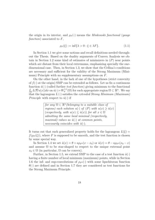
The material of the Thesis is distributed as follows. In Chapter 1 we deal
with a lagrangean of the form L(ξ) = f(ρF (ξ)), where ρF (·) is the Minkowski
functional associated to some convex gauge F. Observe that variational
problems with such type integrands were recently considered in [12], where
the authors proved a comparison theorem assuming the strict convexity of
the gauge F. They constructed a comparison function as a solution of the
associated Euler-Lagrange equation written in the classic divergence form,
essentially using for this the differentiability of the dual Minkowski functional
ρF0 (·), or, in other words, the rotundity of F itself. We do not suppose instead
the set F to be either strictly convex or smooth, or symmetric.
Based on duality arguments of Convex Analysis we obtain first some kinds
of estimates for minimizers close to their nonextremum points and show that
the assumptions of strict convexity and smoothness of f(·) at the origin are
also sufficient and necessary for the validity of the SMP.
Further in this chapter (Sections 1.4 - 1.7) we consider the case when f(·)
is not strictly convex at the origin, and, hence, the SMP in the traditional
sense is no longer valid. We enlarge this property by considering some specific
functions (called test or comparison functions) in the place of identical zero.
14](https://image.slidesharecdn.com/tesefinal-160412170430/85/Tese-Final-net-15-320.jpg)
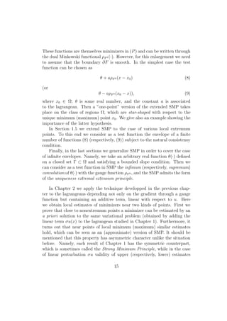
![hold whenever σ > 0 (respectively, σ < 0). Moreover, we observe also a
”cross” effect: the function, which estimates minimizers of the integral with
the perturbation σu is a solution of the variational problem with additive
term −σu. However, all of these effects disappear when σ tends to zero, and
the estimates above reduce to (local) Strong Maximum (Minimum) Principle
in usual sense.
In Chapter 3 we consider the case when the additive term depending on
u is essentially nonlinear. However, due to technical difficulties we assume
lagrangean to be rotationally invariant with respect to the gradient. Namely,
we study the functional
Ω
[f( u(x) ) + g(u(x))] dx (Ig)
where f(·) and g(·) are continuous convex nonnegative functions such that
f(0) = g(0) = 0, ∂g(0) = {0}, and the derivative f (t) is continuous and
tends to zero as t → 0+
. We see that the identical zero is a minimizer
of (Ig) among all Sobolev functions with the zero boundary data, and we
can formulate for (Ig) the SMP in the traditional sense (as in [16]). Notice
that if the functions f(·) and g(·) are more regular (in particular, g(·) is
differentiable), all the minimizers of (Ig) satisfy the Euler-Lagrange equation
div ξf( u(x) ) = g (u(x)),
which is a special case of equations studied by P. Pucci and J. Serrin (see
[53, 54]) and for which a necessary and sufficient condition of the validity of
SMP was found. By using a similar technique combined with the comparison
argument due to A. Cellina we prove that the same condition (divergence of
a kind of improper Riemann integral) is sufficient also for the validity of the
SMP in variational setting even if the respective Euler-Lagrange equation is
no longer valid.
In Conclusion we summarize the obtained results.
16](https://image.slidesharecdn.com/tesefinal-160412170430/85/Tese-Final-net-17-320.jpg)
![Chapter 1
Lagrangeans depending on u
through a gauge function
In this chapter we consider the variational problem
min
Ω
L( u(x)) dx : u(·) ∈ u0
(·) + W1,1
0 (Ω) (P)
where L : Rn
→ R+
∪ {+∞} is a convex lower semicontinuous mapping with
L(0) = 0 and u0
(·) ∈ W1,1
(Ω). In Introduction we already formulated the
Strong Maximum Principle for the problem (P) in the following form (due
to A. Cellina [16]):
given an open bounded connected region Ω ⊂ Rn
an arbitrary admissible continuous nonnegative
solution u (·) of (P) can be equal to zero at some
point x∗
∈ Ω only in the case u ≡ 0.
Recall that admissible solutions of (P) are those which give finite values
to the integral. In the case of rotationally invariant lagrangeans, i.e., L(ξ) =
f( ξ ) with a lower semicontinuous convex function f : R+
→ R+
∪ {+∞},
f(0) = 0, smoothness and strict convexity of the function f (·) at the origin
are necessary and sufficient conditions for the validity of SMP (see [16]).
Here we assume the lagrangean to be symmetric in a more general sense,
namely, L(ξ) = f(ρF (ξ)), where F ⊂ Rn
is a compact convex set containing
17](https://image.slidesharecdn.com/tesefinal-160412170430/85/Tese-Final-net-18-320.jpg)
![whole real line by setting, e.g., f(t) := +∞ for t < 0. It is well known that
v ∈ ∂L(ξ) iff ξ ∈ ∂L∗
(v), and for each ξ ∈ Rn
the equality
∂ρF (ξ) = NF
ξ
ρF (ξ)
∩ ∂F0
(1.4)
holds (see, e.g., Corollary 2.3 in [21]), where ∂F0
is the boundary of F0
, and
NF (ξ) is the normal cone to the set F at ξ ∈ ∂F, i.e., the subdifferential of
the indicator function IF (·) (IF (x) is equal to 0 on F and to +∞ elsewhere).
For the basic facts of Convex Analysis we refer to [49] or to [57]. Let us now
recall only a pair of dual properties, which will be used later on. We say that
the set F is smooth (has smooth boundary) if for each ξ ∈ ∂F there exists a
unique v ∈ NF (ξ) with v = 1. By (1.4) this property is equivalent to the
differentiability of ρF (·) at each ξ = 0. On the other hand, we say that F
is rotund (strictly convex) if for each x, y ∈ ∂F, x = y, and 0 < λ < 1 we
have (1 − λ)x + λy ∈ intF. Given r > 0 and 0 < α < β < 1 let us define the
following modulus of rotundity:
MF (r; α, β) := inf {1 − ρF (ξ + λ (η − ξ)) :
ξ, η ∈ ∂F, ρF (ξ − η) ≥ r; α ≤ λ ≤ β} . (1.5)
Since in a finite-dimensional space a closed and bounded set is compact, the
set F is rotund if and only if MF (r; α, β) > 0 for all r > 0 and 0 < α < β < 1.
The rotundity can be also interpreted in terms of nonlinearity of the gauge
function ρF (·). Namely, F is rotund iff the equality ρF (x+y) = ρF (x)+ρF (y)
holds only in the case when x = λy with λ ≥ 0. It is well-known that the
polar set F0
is rotund if and only if F is smooth.
Since f(0) = 0, f = 0 and domf = {0}, we also have f∗
(0) = 0, f∗
= 0
and domf∗
= {0}. Therefore, due to the elementary properties of convex
functions there exist k, a ∈ [0, +∞) and 0 < b ≤ +∞ such that
∂f(0) = [0, k];
∂f∗
(0) = {t : f(t) = 0} = [0, a]; (1.6)
domf∗
= [0, b] (or [0, b)).
Let us define the function ϕ : [0, b) → R+
by
ϕ(t) := sup ∂f∗
(t) < +∞. (1.7)
20](https://image.slidesharecdn.com/tesefinal-160412170430/85/Tese-Final-net-21-320.jpg)
![It is nondecreasing by monotonicity of the subdifferential. We also introduce
the number γn,f that equals k whenever both n = 1 and f is not affine in a
neighbourhood of zero (i.e., f(t)/t = const near 0), and γn,f = 0 in all other
cases.
For an open bounded connected domain Ω ⊂ Rn
we introduce the func-
tions
r±
(x) = r±
Ω(x) := sup{r > 0 : x ± rF0
⊂ Ω}, x ∈ Ω. (1.8)
We have that
r+
(x) ≤ r+
(y) + ρF0 (y − x) (1.9)
for all x, y ∈ Ω. Indeed, given ε > 0 let us take r > 0 such that
r+
(x) ≤ r + ε (1.10)
and x + rF0
⊂ Ω. Then for each y ∈ Ω due to the convexity of F0
we
successively have
y − x + (r − ρF0 (y − x))F0
⊂ ρF0 (y − x)F0
+ (r − ρF0 (y − x))F0
⊂ rF0
.
Consequently,
y + (r − ρF0 (y − x))F0
⊂ x + rF0
⊂ Ω,
and, hence, r − ρF0 (y − x) ≤ r+
(y). Combining this with (1.10) and taking
into account arbitrarity of ε we arrive at (1.9). Similarly,
r−
(x) ≤ r−
(y) + ρF0 (x − y), (1.11)
x, y ∈ Ω. The inequalities (1.9) and (1.11) imply in particular the Lipschitz
continuity of the functions r±
: Ω → R+
.
Given x0 ∈ Ω the set
St(x0) = StΩ(x0) := {x : [x0, x] ⊂ Ω} (1.12)
is said to be the star in Ω associated to the point x0, where
[x0, x] := {(1 − λ)x0 + λx : 0 ≤ λ ≤ 1}
is the closed segment connecting x0 and x. It follows immediately from (1.12)
that StΩ (x0) is open. The set Ω is said to be star-shaped with respect to
x0 ∈ Ω if Ω = St(x0). For instance, a convex domain Ω is star-shaped with
respect to each point x ∈ Ω. We say also that Ω is densely star-shaped with
respect to x0 if Ω ⊂ St(x0), where over bar means the closure in Rn
.
21](https://image.slidesharecdn.com/tesefinal-160412170430/85/Tese-Final-net-22-320.jpg)
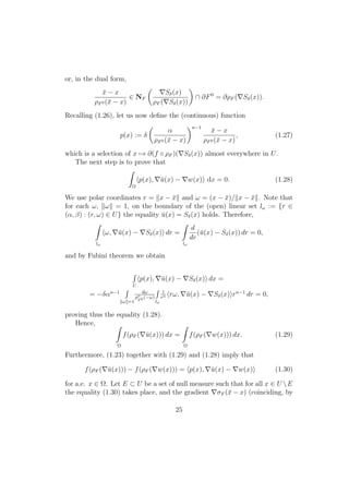
![Proof. (i) If k > 0 but γn,f = 0, i.e., either n > 1 or f (·) is affine near 0,
then the result is trivial because ϕ (η) = 0 for each 0 < η < k.
Let us suppose now k = 0. Then γn,f = 0 and ϕ(t) > 0 for all t > 0.
Since the function ¯u(·) is continuous and ϕ(·) is upper semicontinuous, it
follows from (1.14) that for some small δ > 0 and α ∈ (0, β) the inequality
¯u(x) ≥ µ + ϕ(t)(β − ρF0 (¯x − x)) (1.19)
holds whenever ρF0 (¯x−x) ≤ α and 0 < t ≤ δ. Let us consider the real-valued
function s → ϕ(δ(α
s
)n−1
), which is (Riemann) integrable on the interval [α, β].
Denoting by
Rδ(r) := µ +
β
r
ϕ δ(
α
s
)n−1
ds, (1.20)
we deduce from (1.19) that
¯u(x) ≥ Rδ(ρF0 (¯x − x)) (1.21)
for all x ∈ Ω with ρF0 (¯x − x) = α. Observe that Rδ(β) = µ, and by (1.13)
the inequality (1.21) holds trivially for x ∈ Ω with ρF0 (¯x − x) = β. This
inequality is thus valid on ∂Aα,β, where
Aα,β := {x ∈ Rn
: α ≤ ρF0 (¯x − x) ≤ β}.
Our goal now is to extend this inequality to the interior of Aα,β, using its
validity on the boundary, i.e., to prove a comparison result. Denote by
Sδ(x) := Rδ(ρF0 (¯x − x)) and assume that the (open) set
U := {x ∈ Aα,β : ¯u(x) < Sδ(x)}
is nonempty. Let us extend the Lipschitz continuous function Sδ : Aα,β → R+
to the whole Ω by setting Sδ(x) = Rδ(β) = µ for x ∈ Ω with ρF0 (¯x − x) > β,
and Sδ(x) = Rδ(α) whenever ρF0 (¯x − x) < α. Consider the function w(x) :=
max{¯u(x), Sδ(x)}, which is equal to Sδ(x) on U and to ¯u(x) elsewhere. Let
us show that w(·) minimizes the functional in (PF ) on ¯u(·) + W1,1
0 (Ω, R),
taking into account that ¯u is a solution of (PF ).
Since ¯u(·) is a solution, we have
Ω
[f(ρF ( ¯u(x))) − f(ρF ( w(x)))] dx ≤ 0. (1.22)
23](https://image.slidesharecdn.com/tesefinal-160412170430/85/Tese-Final-net-24-320.jpg)
![If p(·) is an arbitrary (measurable) selection of x → ∂(f ◦ ρF ( w(x))), then,
by definition of the subdifferential of a convex function,
f(ρF ( ¯u(x))) − f(ρF ( w(x))) ≥ p(x), ¯u(x) − w(x) (1.23)
for a.e. x ∈ Ω, and hence
Ω
[f(ρF ( ¯u(x))) − f(ρF ( w(x)))] dx ≥
≥
Ω
p(x), ¯u(x) − w(x) dx. (1.24)
Now we construct a measurable selection p(·) in such a way that the last
integral is equal to zero. Since w(x) = ¯u(x) for a.e. x ∈ Ω U, and
w(x) = Sδ(x) for a.e. x ∈ U (see [41, p. 50]), we choose first p(x) as an
arbitrary measurable selection of the mapping x → ∂(f ◦ ρF )( ¯u(x)) = ∅
on Ω U. On the set U instead we define p(x) according to the differential
properties of Sδ(x). Observe first of all that Rδ(r) = −ϕ(δ(α
r
)n−1
) for all
α < r < β except for at most a countable number of points. Furthermore,
by the Lipschitz continuity of x → ρF0 (¯x − x) the function Sδ(·) is almost
everywhere differentiable on Ω, and
Sδ(x) = −Rδ(ρF0 (¯x − x)) ρF0 (¯x − x) (1.25)
for a.e. x ∈ U. Due to (1.4) the gradient ρF0 (¯x − x) belongs to ∂F, and,
consequently,
ρF ( Sδ(x)) = Rδ(ρF0 (¯x − x)) = ϕ(δ(
α
ρF0 (¯x − x)
)n−1
).
Hence, by the definition of ϕ(·), on one hand, we obtain
δ
α
ρF0 (¯x − x)
n−1
∈ ∂f(ρF ( Sδ(x))) (1.26)
for a.e. x ∈ U. On the other hand (see (1.4) and (1.25)), Sδ (x) is a normal
vector to F0
at the point ¯x−x
ρF 0 (¯x−x)
, that means (see also (1.2))
Sδ(x),
¯x − x
ρF0 (¯x − x)
= σF0 ( Sδ(x)) = ρF ( Sδ(x)),
24](https://image.slidesharecdn.com/tesefinal-160412170430/85/Tese-Final-net-25-320.jpg)
![homogeneity, with σF (p(x)) (see (1.27)) exists. In accordance with (1.30)
both ¯u(x) and w(x) belong to ∂(f ◦ ρF )∗
(p(x)) = ∂(f∗
◦ σF )(p(x)), and
for each x ∈ U E the latter subdifferential admits the form
∂f∗
(ρF0 (p(x))) σF (¯x − x),
where (see (1.27))
ρF0 (p(x)) = δ
α
ρF0 (¯x − x)
n−1
. (1.31)
Notice that there is at most a countable family of disjoint open intervals
J1, J2, ... ⊂ [α, β] such that the real function f(·) is affine on each Ji with a
slope τi > 0, i = 1, 2, ... . In other words, τi are discontinuity points of ϕ(·).
Denoting by Ei := ¯x − α δ
τi
1
n−1
∂F0
we see that for all x /∈
∞
i=1
Ei (the set
of null measure) ∂f∗
(ρF0 (p(x))) is a singleton. So that w(x) = ¯u(x) for
a.e. x ∈ Ω contradicting the assumption U = ∅. Thus, we have proved the
inequality (1.21) on {x ∈ Ω : α ≤ ρF0 (¯x − x) ≤ β}. Combining ( 1.21) and
(1.20) by the mean value theorem we obtain (1.15) with η = δ α
β
n−1
.
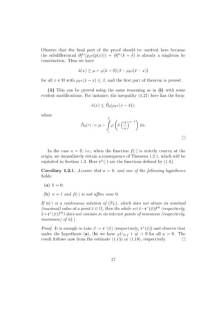
Finally, assume that γn,f = k > 0. In this case n = 1, the function
f(·) admits positive slope at zero but it is not affine near 0 (consequently,
ϕ(k) = 0), and obviously a = 0. Then, for a given β > 0 with ¯x − βF0
⊂ Ω
we have ¯u(¯x) > µ + ϕ(k)β, and, since ¯u(·) and ϕ(·) are continuous, there
exist δ > 0 and 0 < α < β such that
¯u(x) ≥ µ + ϕ(k + t)(β − ρF0 (¯x − x))
for all x ∈ Ω with ρF0 (¯x − x) ≤ α and 0 < t ≤ δ. Taking into account
the monotonicity of the subdifferential ∂f∗
(·) and the nonaffinity of f(·) in
a neighbourhood of zero, we can choose δ > 0 such that ∂f∗
(k + δ) is a
singleton (equivalently, k + δ is a slope of f(·) different from slopes of its
affine pieces near zero). Now we can proceed as in the first part of the proof
by using the comparison argument with the linear function
Rδ(r) := µ + ϕ(k + δ)(β − r), α ≤ r ≤ β.
The selection p(x) ∈ ∂(f ◦ ρF )( (Rδ ◦ ρF0 )(¯x − x)) appearing in the equality
(1.28) takes the form
p(x) = (k + δ)
¯x − x
ρF0 (¯x − x)
.
26](https://image.slidesharecdn.com/tesefinal-160412170430/85/Tese-Final-net-27-320.jpg)
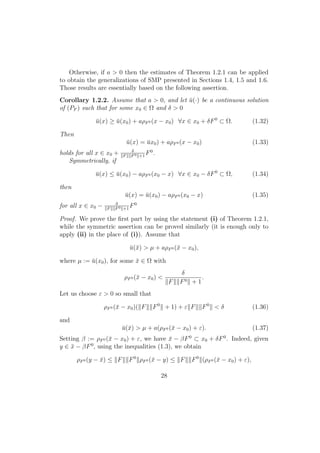
![and it follows from (1.36 ) that
ρF0 (y − x0) ≤ ρF0 (y − ¯x) + ρF0 (¯x − x0) < δ.
In particular, ¯u(x) ≥ µ for all x ∈ ¯x − βF0
. Combining this inequality with
(1.37) by Theorem 1.2.1 (i) we find η > 0 such that
¯u(x) ≥ µ + ϕ(η)(β − ρF0 (¯x − x)) ∀x ∈ ¯x − βF0
. (1.38)
Applying (1.38) to the point x0 ∈ ¯x − βF0
, we obtain finally
¯u(x0) ≥ µ + ϕ(η)ε ≥ µ + aε > µ,
which is a contradiction. The equality (1.33) can be extended then to the
boundary of x0 + δ
F F0 +1
F0
by continuity of the involved functions.
From the latter part of the proof of Theorem 1.2.1 (i) it is easy to see
that in the case n = 1, due to the disconnectedness of the annulus Aα,β,
estimates like (1.15) and (1.18) hold without symmetry. To be more precise,
let us consider a convex (not necessarily even) function L : R → R+
∪ {+∞}
with L(0) = 0 and 0 ∈ int domL, lower semicontinuous on its domain and
such that L(·) is not identically equal to zero on both negative and positive
half-lines. In what follows the set of functions with these properties will be
denoted by L. Given L(·) ∈ L it is obvious that the function L decreases
on ] − ∞, 0[ and increases on ]0, +∞[, that there exist 0 < b±
≤ +∞ with
dom L∗
= {t : −b−
< t < b+
}, where one of the signs ”<” (or both of them)
can be replaced to ”≤”, and that 0 ∈ ∂L(0), 0 ∈ ∂L∗
(0). Consequently,
for some nonnegative (finite) k±
and a±
we have ∂L(0) = [−k−
, k+
] and
∂L∗
(0) = [−a−
, a+
]. As in the symmetric case, let us introduce the upper
semicontinuous nondecreasing function ϕ : (−b−
, b+
) → R by setting ϕ(t) :=
sup ∂L∗
(t). Observe that by monotonicity of the subdifferential, one of the
numbers k+
or a+
(analogously, k−
or a−
) is always equal to zero. The
following statement contains the one-sided estimates for solutions of the one-
dimensional problem (PF ). For the sake of simplicity we consider here only
the case of local minimum. One easily makes the respective modifications
when the symmetric conditions (of local maximum) take place.
Theorem 1.2.2. Let L ∈ L, and let ¯u(·) be a continuous solution of (PF ).
Assume that a point ¯x ∈ Ω and numbers µ ∈ R, β > 0 are such that
¯u(x) ≥ µ ∀x ∈ [¯x − β, ¯x] ⊂ Ω (1.39)
29](https://image.slidesharecdn.com/tesefinal-160412170430/85/Tese-Final-net-30-320.jpg)
![and
¯u(¯x) > µ + a+
β. (1.40)
If L is not affine in a right-hand neighbourhood of zero then there exists η > 0
such that
¯u(x) ≥ µ + ϕ(k+
+ η)(β + x − ¯x) ∀x ∈ [¯x − β, ¯x]. (1.41)
Analogously, if L is not affine in a left-hand neighbourhood of zero and the
relations (1.39), (1.40) are substituted by the following:
¯u(x) ≥ µ ∀x ∈ [¯x, ¯x + β] ⊂ Ω;
¯u(¯x) > µ + a−
β,
then for some η > 0
¯u(x) ≥ µ − ϕ(−k−
− η)(β + ¯x − x) ∀x ∈ [¯x, ¯x + β]. (1.42)
Proof. We use here the same arguments as in the proof of Theorem 1.2.1.
Let us emphasize only some simplifications in the main steps that have a
methodical interest. Let us consider the first case (L(·) is not affine on the
right side of the origin, and (1.39), (1.40) are fulfilled). We write (1.40) as
¯u(¯x) > µ + ϕ(k+
)β and by the upper semicontinuity of ϕ(·) choose η > 0 so
small that the latter inequality holds with ϕ(k+
+ η) in the place of ϕ(k+
).
Assume also (see the last part of the proof of Theorem 1.2.1 (i)) that the
subdifferential ∂L∗
(k+
+η) is a singleton, namely, ∂L∗
(k+
+η) = {ϕ(k+
+η)}.
Here we use the nonaffinity of L(·) on the right side of zero. Defining on Ω
the continuous function
Rδ(x) :=
µ if x < ¯x − β,
µ + ϕ(k+
+ η)(β + x − ¯x) if ¯x − β ≤ x ≤ ¯x,
µ + ϕ(k+
+ η)β if x > ¯x,
we wish to prove that ¯u(x) ≥ Rδ(x) for all x ∈ [¯x − β, ¯x]. If this inequality
is violated in some (open) set U ⊂ (¯x − β, ¯x) then by the Newton-Leibnitz
formula
Ω
(¯u (x) − w (x)) dx =
U
(¯u (x) − Rδ(x)) dx = 0, (1.43)
where w(x) := max{¯u(x), Rδ(x)}. Since k+
+ η ∈ ∂L(Rδ(x)), we have
L(¯u (x)) − L(w (x)) ≥ (k+
+ η)(¯u (x) − w (x)) (1.44)
30](https://image.slidesharecdn.com/tesefinal-160412170430/85/Tese-Final-net-31-320.jpg)
![Then for each open bounded connected region Ω ⊂ Rn
there is no continuous
admissible nonconstant minimizer of
u (·) →
Ω
L ( u (x)) dx (1.45)
on u0
(·) + W1,1
0 (Ω) for u0
(·) ∈ W1,1
(Ω), which admits its minimal (or max-
imal) value in Ω.
Proof. Observe first that in the framework of the condition (i) the hypothesis
(H1) holds automatically, while (H2) can be violated. An open bounded
connected set in this case is an interval Ω = (A, B) with A < B. Assuming
that ¯u(·) is a minimizer of (1.45), and ¯x ∈ Ω is such that ¯u(¯x) > µ :=
min
Ω
¯u(x), we put β := ¯x − A and obtain by Theorem 1.2.2 that ¯u(x) >
µ for all x ∈ (A, ¯x] (because in (1.41) we have ϕ(k+
+ η) > 0 ∀η > 0).
Analogously, by using the estimate (1.42) of Theorem 1.2.2, we conclude
that ¯u(x) > µ ∀x ∈ [¯x, B). Consequently, there are only two possibilities:
either the minimum of ¯u(·) is attained in one of the end-points of the segment
[A, B] or ¯u ≡ µ on Ω. In the case of maximum the reasoning is similar.
Let us suppose now condition (ii). Take an arbitrary continuous admis-
sible function ¯u : Ω → R that minimizes the integral (1.45), and let µ be
its minimum on Ω. If ¯u(·) is not constant then the (open) set W := {x ∈
Ω : ¯u (x) = µ} is nonempty. Since a = 0, it follows from Corollary 1.2.1
that ¯x − βF0
⊂ W whenever ¯x ∈ W, 0 < β < r−
(¯x) (see (1.8)). Fix
now x∗
∈ W (closure of W in Ω). By the continuity let us choose an arbi-
trary 0 < ε < 1
2 F
r−
(x∗
) so small that r−
(x∗
) ≤ 2r−
(x) for all x ∈ Ω with
x − x∗
≤ ε. Let ¯x ∈ W ∩ x∗
+ εB . Then ¯x ∈ W and
ρF0 (¯x − x∗
) ≤ ε F <
1
2
r−
(x∗
) ≤ r−
(¯x) .
Hence, x∗
also belongs to W, and W is closed in Ω, implying that W = Ω
because Ω is connected. Thus, the open region Ω is free from the points of
mimimum of ¯u(·). Analogously, ¯u(·) being non constant can not attain in Ω
its maximum, and SMP is proved. Notice that here we use the argument in
some sense dual to the classical proof for harmonic functions (see, e.g., [36,
p. 15]).
32](https://image.slidesharecdn.com/tesefinal-160412170430/85/Tese-Final-net-33-320.jpg)
![As an example of the functional, for which the validity of SMP follows
from Theorem 1.3.1 but is not covered by earlier results, we consider the
integral
Ω
n
i=1
∂u
∂xi
2
dx.
Here f(t) = t2
and ρF (·) is the l1-norm in Rn
. Observe that the set
F = {x ∈ Rn
:
n
i=1
xi ≤ 1}
in this case is neither smooth, nor strictly convex.
The Strong Maximum Principle is not valid if the hypothesis (H1) does
not hold because, as shown in [19], there are many (Lipschitz) continuous
nonnegative (nonpositive) minimizers of (1.45) with the trivial boundary
condition u0 (x) = 0, which touch the zero level at interior points of Ω as well.
If (H2) is violated then in the case n > 1 one can construct a counterexample
to SMP based on the same arguments as those in [16]. Indeed, fix arbitrary
¯x ∈ Rn
, µ ∈ R and define
Ω := {x ∈ Rn
: α < ρF0 (¯x − x) < β}
for some β > α > 0. Then for each δ > 0 the function Sδ(x) := Rδ(ρF0 (¯x−x))
(see (1.20)) is a solution of (PF ) (here ∂f(0) = [0, k], k > 0) with u0
(x) =
Sδ(x) in virtue of the relations (1.28) and (1.23), where w(·) = Sδ(·), U = Ω,
¯u(·) is another minimizer, and the mapping p(·) is given by (1.27). Clearly,
µ = min
x∈Ω
Sδ(x), and it is enough only to choose δ > 0, α and β such that
Rδ(α) > µ and Rδ(r) = µ for β −ε ≤ r ≤ β, where ε > 0 is sufficiently small.
Let, for instance, β = 2α and k < δ < 2n−1
k (observe the importance of the
condition n > 1 for this construction). Then for some 0 < ε < β − α
δ
α
α + ε
n−1
> k, δ
α
2α − ε
n−1
< k
and, consequently,
Rδ(α) ≥ µ +
α+ε
α
ϕ δ
α
s
n−1
ds ≥ µ + ϕ δ
α
α + ε
n−1
ε > µ,
33](https://image.slidesharecdn.com/tesefinal-160412170430/85/Tese-Final-net-34-320.jpg)
![while for β − ε ≤ r ≤ β we have
µ ≤ Rδ(r) ≤ µ +
β
β−ε
ϕ δ
α
s
n−1
ds ≤ µ + ϕ δ
α
2α − ε
n−1
ε = µ.
We use here the fact that ϕ(t) ≡ 0 on [0, k] and ϕ(t) > 0 for t > k. Thus
Sδ (·) is a nonconstant continuous solution of (PF ) admitting its minimum at
each point x ∈ Ω with β − ε ≤ ρF0 (¯x − x) ≤ β, which contradicts SMP.
The function L(·) may have a nontrivial slope at zero, which is different
from the slopes at all points x = 0. Let us give a simple example of such
function, which, moreover, is neither strictly convex nor smooth near the
origin.
Example 1. Fix an arbitrary strictly decreasing sequence {τm} ⊂ (0, π/2)
converging to zero, and define the continuous function f : (0, π/2) → R+
,
which is equal to tgt for t = τm, m = 1, 2, ..., and for τ1 < t < π/2, and
affine on each interval (τm+1, τm). We set also f(t) = +∞ for t ≥ π/2.Then
∂f(0) = [−1, 1] but, nevertheless, the Strong Maximum Principle is valid for
the functional
Ω
f( u (x) ) dx due to Theorem 1.3.1.
However, even in the case n = 1 the function f(·) can not be affine near
the origin.
Example 2. If f(t) = kt for 0 ≤ t ≤ ε then for each admissible function
u(·) ∈ W1,1
(0, 1) with the boundary values u(0) = 0 and u(1) = ε/2 we have
by Jensen’s inequality
1
0
f( u (x) ) dx ≥ f(
1
0
u (x) dx ) =
kε
2
=
1
0
f( ¯u (x) ) dx,
where ¯u(x) := ε
2
x, x ∈ [0, 1]. On the other hand, the function ˜u(x) equal to 0
on 0, 1
2
and to εx− ε
2
on 1
2
, 1 gives the same minimal value to the integral.
34](https://image.slidesharecdn.com/tesefinal-160412170430/85/Tese-Final-net-35-320.jpg)
![1.4 A one-point extended Strong Maximum
Principle
The traditional Strong Maximum Principle is no longer valid if L = f ◦ ρF
with ∂f∗
(0) = {0}. However, also in this case we can consider a similar
property, which clearifies the structure of minimizers of the functional (PF )
and has the same field of applications as the classical SMP. Let us start with
the one-point SMP when a test function admits a unique point of local min-
imum (maximum). Setting ˆu(x) = µ + aρF0 (x − x0) with µ ∈ R and x0 ∈ Ω,
it was already shown (see Corollary 1.2.2) that for an arbitrary minimizer
¯u(·), ¯u(x0) = µ, of (PF ) the inequality ¯u(x) ≥ ˆu(x) valid on a neighbourhood
of x0 becomes, in fact, the equality on another (may be smaller) neighbour-
hood. First we show that this property can be extended to the maximal
homothetic set x0 + rF0
contained in Ω.
Theorem 1.4.1. Assume that L = f ◦ ρF , where f : R+
→ R+
∪ {+∞} is
a convex lower semicontinuous function, f(t) = 0 iff t ∈ [0, a], a > 0, and
F ⊂ Rn
is a convex closed bounded set with 0 ∈ intF. Let Ω ⊂ Rn
be an
open bounded domain, x0 ∈ Ω and ¯u(·) be a continuous solution of (PF ). If
¯u(x) ≥ ¯u(x0) + aρF0 (x − x0) (1.46)
for all x ∈ x0 + r+
(x0) F0
then the equality
¯u (x) = ¯u (x0) + aρF0 (x − x0) (1.47)
holds on x0 + r+
(x0) F0
. Analogously, if
¯u (x) ≤ ¯u (x0) − aρF0 (x0 − x) (1.48)
for all x ∈ x0 − r−
(x0) F0
, then the equality
¯u (x) = ¯u (x0) − aρF0 (x0 − x) (1.49)
holds on x0 − r−
(x0) F0
.
35](https://image.slidesharecdn.com/tesefinal-160412170430/85/Tese-Final-net-36-320.jpg)
![Therefore, ¯v(·) is a solution of (PF ) with u0
(·) = ¯v(·).
Let x0 be a unique point from [x0, ¯x] such that ρF0 (x0 − x0) = R. Namely,
x0 = x0 + λ (¯x − x0) where 0 < λ := R
ρF 0 (¯x−x0)
< 1. Setting now β :=
ρF0 (¯x − x0) + ε, by (1.54) we obtain
¯v (¯x) ≥ ¯u (¯x) > ¯u (x0) + aρF0 (x0 − x0) +
+ a (ρF0 (¯x − x0) + ε) = µ + aβ. (1.57)
On the other hand, the inequality ρF0 (¯x − x) ≤ β implies that
ρF0 (x − x0) ≤ ρF0 (x − ¯x) + ρF0 (¯x − x0) + ρF0 (x0 − x0) ≤
≤ F F0
ρF0 (¯x − x) + ρF0 (¯x − x0) + R ≤
≤ F F0
+ 1 ρF0 (¯x − x0) +
+ ε F F0
+ R. (1.58)
Since obviously ρF0 (¯x − x0) < δ, we obtain from (1.58) and (1.53) that
ρF0 (x − x0) < r+
(x0). Hence, by the definition of ¯v (·)
¯v (x) ≥ µ ∀x ∈ ¯x − βF0
. (1.59)
The inequalities (1.59) and (1.57) allow us to apply Theorem 1.2.1 with the
solution ¯v (·) in the place of ¯u (·) and to find η > 0 such that
¯v (x) ≥ µ + ϕ (η) (β − ρF0 (¯x − x)) ∀x ∈ ¯x − βF0
.
In particular, for x = x0 ∈ ¯x − βF0
we have
¯v (x0) ≥ µ + ϕ (η) ε > µ. (1.60)
However, by the definition of R (see (1.50))
¯u (x0) = ¯u (x0) + aρF0 (x0 − x0) = µ.
Thus ¯v (x0) = µ as well, contradicting the strict inequality (1.60).
In the case when the Minkowski functional ρF (·) is differentiable, the
latter extremality result can be extended to arbitrary (densely) star-shaped
domains in the place of ρF0 -balls x0 ± rF0
.
37](https://image.slidesharecdn.com/tesefinal-160412170430/85/Tese-Final-net-38-320.jpg)
![Theorem 1.4.2. Assume that the lagrangean L(·) is such as in Theorem
1.4.1 with a convex compact and smooth set F ⊂ Rn
, 0 ∈ intF; that Ω ⊂ Rn
is an open bounded region and x0 ∈ Ω. Then for each continuous solution
¯u (·) of (PF ) and each open ˆΩ ⊂ Ω, which is densely star-shaped w.r.t. x0,
the inequality (1.46) (respectively, (1.48)) holds for all x ∈ ˆΩ if and only if
the equality (1.47) (respectively, (1.49)) is valid on ˆΩ.
Proof. As earlier we prove here only the implication (1.46)⇒(1.47), while
the other one ((1.48)⇒(1.49)) can be treated similarly. Moreover, it is
enough to prove the equality (1.47) on the star StˆΩ (x0), because to each
x ∈ ˆΩ StˆΩ (x0) ⊂ StˆΩ (x0) it can be extended by continuity of the involved
functions.
Let us assume validity of (1.46) on ˆΩ and fix ¯x ∈ StˆΩ (x0). By the
compactness we choose ε > 0 such that
[x0, ¯x] ± εF0
⊂ ˆΩ. (1.61)
Set
δ := 2εMF0
2ε
∆
;
ε
ε + ∆
,
∆
ε + ∆
, (1.62)
where MF0 is the rotundity modulus defined by (1.5) and ∆ is the ρF0 -
diameter of the domain ˆΩ, i.e.,
∆ := sup
ξ,η∈ˆΩ
ρF0 (ξ − η) > 0. (1.63)
It follows from the remarks of Section 1.1 that F0
is rotund, and therefore
δ > 0. Let us consider an uniform partition of the segment [x0, ¯x] by the
points
xi := x0 + ih
¯x − x0
ρF0 (¯x − x0)
,
i = 0, 1, ..., m, with
h :=
ρF0 (¯x − x0)
m
≤ min
ε
√
M
,
δ
M
, (1.64)
where M := ( F F0
+ 1)
2
. Since the inequality (1.46) holds for all x ∈
x0 + εF0
(see (1.61)) and ρF0 (x1 − x0) = h ≤ ε
F F0 +1
, it follows from
Corollary 1.2.2 that
¯u (x1) = ¯u (x0) + aρF0 (x1 − x0) = ¯u (x0) + ah.
38](https://image.slidesharecdn.com/tesefinal-160412170430/85/Tese-Final-net-39-320.jpg)
![We want to prove by induction in i that
¯u (xi) = ¯u (x0) + iah, (1.65)
i = 1, 2, ..., m. Then for i = m we will have
¯u (¯x) = ¯u (xm) = ¯u (x0) + aρF0 (¯x − x0) ,
and theorem will be proved due to arbitrarity of ¯x ∈ StˆΩ (x0). So, we assume
that (1.65) is true for some i with 1 ≤ i ≤ m − 1 and define the function
¯ui : Ω → R as
max {¯u (x) , min {¯u (xi) + aρF0 (x − xi) , µi − aρF0 (xi − x)}} (1.66)
on ˆΩ and as ¯u (x) elsewhere. Here
µi := ¯u (x0) + a (i + M) h. (1.67)
Let us devide the remainder of the proof in three steps.
Step 1. We claim first that for each x /∈ [x0, ¯x] ± εF0
the inequality
ρF0 (x − x0) + ρF0 (xi − x) − ρF0 (xi − x0) ≥ δ (1.68)
holds. Indeed, given such a point x we have
ρ0 := ρF0 (x − x0) ≥ ε and ρi := ρF0 (xi − x) ≥ ε.
On the other hand, clearly ρ0 ≤ ∆ and ρi ≤ ∆ (see (1.63)). Hence, by the
monotonicity
λ :=
ρ0
ρ0 + ρi
∈
ε
∆ + ε
,
∆
∆ + ε
. (1.69)
Furthermore,
ρF0 (x − x0) + ρF0 (xi − x) − ρF0 (xi − x0) =
= (ρ0 + ρi) 1 − ρF0
ρi
ρ0 + ρi
xi − x
ρi
+
ρ0
ρ0 + ρi
x − x0
ρ0
≥
≥ 2ε [1 − ρF0 (ξ + λ (η − ξ))] , (1.70)
where ξ := xi−x
ρi
and η := x−x0
ρ0
. Since
ξ − η =
1
ρ0
+
1
ρi
ρ0
ρ0 + ρi
xi +
ρi
ρ0 + ρi
x0 − x ,
39](https://image.slidesharecdn.com/tesefinal-160412170430/85/Tese-Final-net-40-320.jpg)
![by the choice of x we obtain
ρF0 (ξ − η) ≥
1
ρ0
+
1
ρi
ε ≥
2ε
∆
. (1.71)
Joining together (1.69)-(1.71), (1.62) and the definition of the rotundity mod-
ulus (1.5) we immediately arrive at (1.68).
Step 2. Let us show that ¯ui (·) is the continuous minimizer of the func-
tional in (PF ) on ¯u (·) + W1,1
0 (Ω). Given x ∈ ˆΩ with x /∈ [x0, ¯x] ± εF0
it
folows from (1.68) and (1.64) that
ρF0 (x − x0) + ρF0 (xi − x) ≥ δ + ih ≥ (i + M) h. (1.72)
Since ¯u (x) ≥ ¯u (x0) + aρF0 (x − x0) by the condition, we deduce from (1.72)
and (1.67) that ¯u (x) ≥ µi − aρF0 (xi − x). Consequently, ¯ui (x) = ¯u (x) (see
(1.66)). Due to (1.61) this means continuity of the function ¯ui (·). Besides
that obviously ¯ui (·) ∈ ¯u (·) + W1,1
0 (Ω). We see from (1.66) that for each
x ∈ Ω with ¯ui (x) = ¯u (x) the gradient ¯ui (x) belongs to aF, and therefore
f (ρF ( ¯ui (x))) = 0. By the same argument as in the proof of Theorem 1.4.1
(see (1.56)) ¯ui (·) gives the minimum to (PF ) among all the functions with
the same boundary data.
Step 3. Here we prove that for each x with
ρF0 (x − xi) ≤ F F0
+ 1 h (1.73)
(such x belong to ˆΩ by (1.61) and (1.64)) the inequality
¯ui (x) ≥ ¯ui (xi) + aρF0 (x − xi) (1.74)
holds. Indeed, it follows from (1.73) and (1.3) that
ρF0 (x − xi) + ρF0 (xi − x) ≤ Mh, (1.75)
and taking into account the definition of µi (see (1.67)) and the induction
hypothesis (1.65) we obtain from (1.75) that
¯u (xi) + aρF0 (x − xi) ≤ µi − aρF0 (xi − x) ,
i.e., the minimum in (1.66) is equal to ¯u (xi) + aρF0 (x − xi). This implies
(1.74) because
40](https://image.slidesharecdn.com/tesefinal-160412170430/85/Tese-Final-net-41-320.jpg)
![In what follows by St (x0) we intend the star associated with the point x0
in the domain Ω. It is obvious that x ∈ Ω St (x0) if and only if the segment
[x0, x] meets the ball ¯x + rB, or, in other words, the quadratic equation
x0 + λ (x − x0) − ¯x 2
= λ2
x − x0
2
−
−2λ x − x0, ¯x − x0 + ¯x − x0
2
= r2
(1.78)
has (one or two) roots both belonging to the interval (0, 1). We write the
condition of resolvability of (1.78) as
D (x) := x − x0, ¯x − x0
2
− x − x0
2
¯x − x0
2
− r2
≥ 0 (1.79)
and denote by
λ± (x) :=
x − x0, ¯x − x0 ± D (x)
x − x0
2 (1.80)
its roots. Taking into account continuity of all the involved functions we have
Ω := int (Ω St (x0)) = {x ∈ Σ : D (x) > 0 and
0 < λ− (x) < λ+ (x) < 1} (1.81)
and
E := ∂ (Ω St (x0)) ∩ ∂ (St (x0)) =
= x ∈ Σ : D (x) = 0 and 0 < λ± (x) = x−x0,¯x−x0
x−x0
2 < 1 . (1.82)
The open set Ω is clearly nonempty since it contains, e.g., all the points
¯x + (r + δ) ¯x−x0
¯x−x0
with δ > 0 small enough. For each x ∈ E let us define the
”trace” operator
Φ (x) := x0 + λ± (x) (x − x0) , (1.83)
which is continuous and satisfies the following ”cone” property: if x ∈ E and
x = x0 + λ (x − x0) ∈ Ω with λ > λ± (x) then also x ∈ E and Φ (x ) =
Φ (x). Indeed, we find from (1.79) and (1.80) that D (x ) = λ2
D (x) = 0 and
λ± (x ) = 1
λ
λ± (x) ∈ (0, 1). Hence x ∈ E and the equality Φ (x ) = Φ (x)
follows directly from (1.83). This property and continuity of Φ (·) imply that
the image C := Φ (E) is a compact subset of {x ∈ Ω : x − ¯x = r}.
Define the function ¯u : Ω → R by
¯u (x) :=
ainf
y∈C
{ρF0 (x − y) + ρF0 (y − x0)} if x ∈ Ω St (x0) ,
aρF0 (x − x0) if x ∈ St (x0) ,
(1.84)
42](https://image.slidesharecdn.com/tesefinal-160412170430/85/Tese-Final-net-43-320.jpg)
![and show, first, its continuity. To this end it is enough to verify the equality
inf
y∈C
{ρF0 (x − y) + ρF0 (y − x0)} = ρF0 (x − x0) (1.85)
for each point x ∈ E. Notice that the inequality ”≥” in (1.85) is obvious. In
order to prove ”≤” let us take an arbitrary x ∈ E and put y := Φ (x) = x0 +
λ± (x) (x − x0). Then ρF0 (y − x0) = λ± (x) ρF0 (x − x0) and ρF0 (x − y) =
(1 − λ± (x)) ρF0 (x − x0). So that the inequality ”≤” in (1.85) immediately
follows. The function ¯u (·) is, moreover, lipschitzean on Ω, and its Clarke
subdifferential ∂c
¯u (x) is always contained in aF (see [20, p.92]).
Since by Rademaher’s Theorem the gradient ¯u (x) a.e. exists and
¯u (x) ∈ ∂c
¯u (x), we have f (ρF ( ¯u (x))) = 0 for a.e. x ∈ Ω, and, con-
sequently, ¯u (·) is a solution of (PF ).
The inequality (1.77) is obvious (here ¯u (x0) = 0). Fix now x ∈ Ω and
y ∈ C = Φ (E). Then y = x0 + λ± (z) (z − x0) with some z ∈ E. Assuming
that there exists λ > 0 with x − y = λ (y − x0) and taking into account the
representation of y, we have x = x0 + µ (z − x0) with µ := (λ + 1) λ± (z) >
λ± (z). Due to the ”cone” property of the ”trace” operator (see above) x ∈ E
as well, which is a contradiction. Thus, by the rotundity of the set F0
the
strict inequality
ρF0 (x − y) + ρF0 (y − x0) > ρF0 (x − x0)
holds. Finally, by the compactness of the set C and by arbitrarity of y ∈ C
we conclude that the inequality (1.77) is strict whenever x ∈ Ω , and the
construction is complete.
The method used in Example 3 can be essentially sharpened in order
to cover the case of an arbitrary domain Ω, in which an open subset is not
linearily attainable from x0 ∈ Ω. So, let us formulate the following conjecture.
Conjecture The condition Ω ⊂ St (x0) is necessary for validity of the
one-point Strong Maximum Principle w.r.t. x0 ∈ Ω as given by Corollary
1.4.1.
1.5 A multi-point version of SMP
The one-point version of SMP given in the previous section (see Corollary
1.4.1) can be easily extended to the case when the test function ˆu (·) has a
43](https://image.slidesharecdn.com/tesefinal-160412170430/85/Tese-Final-net-44-320.jpg)
![finite number of local minimum (maximum) points. Namely, let xi ∈ Rn
,
i = 1, ..., m, be different, m ∈ N, and arbitrary real numbers θ1, θ2, ..., θm be
such that the compatibility condition
θi − θj < aρF0 (xi − xj) , i = j, (1.86)
is fulfilled. Considering the functions
ˆu+
(x) := min
1≤i≤m
{θi + aρF0 (x − xi)} (1.87)
and
ˆu−
(x) := max
1≤i≤m
{θi − aρF0 (xi − x)} , (1.88)
we deduce immediately from (1.86) that ˆu+
(xi) = ˆu−
(xi) = θi, i = 1, ..., m,
and that {x1, x2, ..., xm} is the set of all local minimum (maximum) points
of the function (1.87) or (1.88), respectively.
Before proving the main statement (Theorem 1.5.1) let us give some prop-
erty of minimizers in (1.87) (respectively, maximizers in (1.88)), which ex-
tends a well-known property of metric projections. Since it will be used in
the next sections as well, we formulate the following assertion in the form
convenient for both situations.
Lemma 1.5.1. Let Γ ⊂ Rn
be a nonempty closed set and θ (·) be a real-
valued function defined on Γ. Given x ∈ Rn
Γ assume that the minimum
of the function y → θ (y) + aρF0 (x − y) (respectively, the maximum of y →
θ (y) − aρF0 (y − x)) on Γ is attained at some point ¯y ∈ Γ. Then ¯y continues
to be a minimizer of y → θ (y) + aρF0 (xλ − y) (respectively, a maximizer of
y → θ (y) − aρF0 (y − xλ)) for all λ ∈ [0, 1], where xλ := (1 − λ) x + λ¯y.
Proof. Given λ ∈ [0, 1] and y ∈ Γ we obviously have x−y = xλ−y+λ (x − ¯y),
and by the semilinearity
ρF0 (x − y) ≤ ρF0 (xλ − y) + λρF0 (x − ¯y) . (1.89)
Since θ (¯y) + aρF0 (x − ¯y) ≤ θ (y) + aρF0 (x − y), it follows from (1.89) that
θ (¯y) + a (1 − λ) ρF0 (x − ¯y) ≤ θ (y) + aρF0 (xλ − y) .
This proves the first assertion because (1 − λ) (x − ¯y) = xλ − ¯y. The second
case can be easily reduced to the first one by changing the signs.
44](https://image.slidesharecdn.com/tesefinal-160412170430/85/Tese-Final-net-45-320.jpg)
![Strong Maximum Principle proposed by A. Cellina and the extended Strong
Maximum Principle, which we studied in Sections 1.4 and 1.5.
Namely, given an arbitrary real function θ (·) defined on a closed subset
Γ ⊂ Ω and satisfying a natural slope condition w.r.t. F:
θ (x) − θ (y) ≤ aρF0 (x − y) ∀x, y ∈ Γ,. (1.91)
we prove that the inf-convolution
u+
Γ,θ (x) := inf
y∈Γ
{θ (y) + aρF0 (x − y)} (1.92)
(respectively, the sup-convolution
u−
Γ,θ (x) := sup
y∈Γ
{θ (y) − aρF0 (y − x)} ) (1.93)
is the only continuous minimizer u (·) in the problem (PF ) such that u (x) =
θ (x) on Γ and u (x) ≥ u+
Γ,θ (x) (respectively, u (x) ≤ u−
Γ,θ (x)), x ∈ Ω.
As standing hypotheses in what follows we assume that F is convex closed
bounded and smooth with 0 ∈ intF, and that Ω is an open convex bounded
region in Rn
.
Observe that the function u±
Γ,θ (·) is the minimizer in (PF ) with u0
(x) =
u±
Γ,θ (x). Indeed, it is obviously Lipschitz continuous on Ω, and for its (classic)
gradient u±
Γ,θ existing almost everywhere by Rademacher’s theorem we have
u±
Γ,θ (x) ∈ ∂c
u±
Γ,θ (x) ⊂ aF
for a.e. x ∈ Ω (see [20, Theorem 2.8.6]). Here ∂c
stands for the Clarke’s
subdifferential. Consequently,
f ρF u±
Γ,θ (x) = 0
a.e. on Ω, and the function u±
Γ,θ (·) gives to (PF ) the minimal possible value
zero.
Due to the slope condition (1.91) it follows that u±
Γ,θ (x) = θ (x) for all
x ∈ Γ. Moreover, u±
Γ,θ (·) is the (unique) viscosity solution of the Hamilton-
Jacobi equation
± (ρF ( u (x)) − a) = 0, u |Γ = θ,
(see, e.g., [11]).
46](https://image.slidesharecdn.com/tesefinal-160412170430/85/Tese-Final-net-47-320.jpg)
![Notice that Γ can be a finite set, say {x1, x2, ..., xm} . In this case θ (·)
associates to each xi a real number θi, i = 1, ..., m, and the condition (1.91)
slightly strengthened (by assuming that the inequality in (1.91) is strict for
xi = xj) means that all the simplest test functions θi +aρF0 (x − xi) (respec-
tively, θi − aρF0 (xi − x)) are essential (not superfluous) in constructing the
respective lower or upper envelope. Then the extremal property established
in Section 1.7 is reduced to the extended SMP of Section 1.5 (see Theorem
1.5.1).
On the other hand, if θ (·) is a Lipschitz continuous function defined on
a closed convex set Γ ⊂ Ω with nonempty interior then (1.91) holds iff
θ (x) ∈ aF
for a.e. x ∈ Γ. This immediately follows from Lebourg’s mean value theorem
(see [20, p. 41]) recalling the properties of the Clarke’s subdifferential and
from the separability theorem.
Certainly, the mixed (discrete and continuous) case can be considered as
well, and all the situations are unified by the hypothesis (1.91).
In the particular case θ ≡ 0 ((1.91) is trivially fulfilled) the function
u+
Γ,θ (x) is nothing else than the minimal time necessary to achieve the closed
set Γ from the point x ∈ Ω by trajectories of the differential inclusion with
the constant convex right-hand side
−a ˙x (t) ∈ F0
, (1.94)
while −u−
Γ,θ (x) is, contrarily, the minimal time, for which trajectories of
(1.94) arrive at x starting from a point of Γ. Furthermore, if F = B then
the gauge function ρF0 (·) is the euclidean norm in Rn
, and we have
u±
Γ,θ (x) = ±adΓ (x)
where dΓ (·) means the distance from a point to the set Γ.
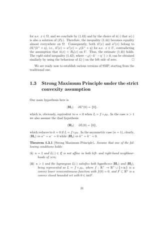
1.7 Generalized Strong Maximum Principle
Now we are ready to deduce the extremal property of the functions u±
Γ,θ (·)
announced above.
47](https://image.slidesharecdn.com/tesefinal-160412170430/85/Tese-Final-net-48-320.jpg)
![Passing to infimum in (1.97) we prove the inequality ”≤” in (1.95) as well.
Since for arbitrary x, y ∈ Γ+
and for y∗
∈ Γ satisfying (1.96) we have
¯u (x) − ¯u (y) = u+
Γ,θ (x) − u+
Γ,θ (y) ≤
≤ aρF0 (x − y∗
) − aρF0 (y − y∗
) ≤ aρF0 (x − y) , (1.98)
we can extend the function θ : Γ → R to the (closed) set Γ+
⊂ Ω by setting
θ (x) = ¯u (x) , x ∈ Γ+
,
and all the conditions on θ (·) remain valid (see (1.98) and (1.95)). So,
without loss of generality we can assume that the strict inequality
¯u (x) > u+
Γ,θ (x) (1.99)
holds for all x ∈ Ω Γ = ∅.
Notice that the convex hull K := co Γ is the compact set contained in Ω
(due to the convexity of Ω). Let us choose now ε > 0 such that K ±εF0
⊂ Ω
and denote by
δ := 2ε MF0
2ε
∆
;
ε
ε + ∆
,
∆
ε + ∆
> 0,
where as usual MF0 is the modulus of rotundity associated to F0
(see 1.5)
and
∆ := sup
ξ,η∈Ω
ρF0 (ξ − η) .
Similarly as in Step 1 in the proof of Theorem 1.4.2 we show that
ρF0 (y1 − x) + ρF0 (x − y2) − ρF0 (y1 − y2) ≥ δ (1.100)
whenever y1, y2 ∈ Γ and x ∈ Ω [(K + εF0
) ∪ (K − εF0
)]. Indeed, we obvi-
ously have
ε ≤ ρ1 := ρF0 (y1 − x) ≤ ∆ and ε ≤ ρ2 := ρF0 (x − y2) ≤ ∆,
and, consequently,
λ :=
ρ2
ρ1 + ρ2
∈
ε
ε + ∆
,
∆
ε + ∆
. (1.101)
49](https://image.slidesharecdn.com/tesefinal-160412170430/85/Tese-Final-net-50-320.jpg)
![Setting ξ1 := y1−x
ρ1
and ξ2 := x−y2
ρ2
we can write
ξ1 − ξ2 =
1
ρ1
+
1
ρ2
ρ2
ρ1 + ρ2
y1 +
ρ1
ρ1 + ρ2
y2 − x ,
and hence
ρF0 (ξ1 − ξ2) ≥
1
ρ1
+
1
ρ2
ε ≥
2ε
∆
. (1.102)
On the other hand,
ρF0 (y1 − x) + ρF0 (x − y2) − ρF0 (y1 − y2)
= (ρ1 + ρ2) 1 − ρF0
ρ1
ρ1 + ρ2
ξ1 +
ρ2
ρ1 + ρ2
ξ2 ≥
≥ 2ε [1 − ρF0 (ξ1 + λ (ξ2 − ξ1))] . (1.103)
Combining (1.103), (1.102), (1.101) and the definition of the rotundity mod-
ulus we arrive at (1.100).
Let us fix ¯x ∈ Ω Γ and ¯y ∈ Γ such that
u+
Γ,θ (¯x) = θ (¯y) + aρF0 (¯x − ¯y) .
Then by Lema 1.5.1 the point ¯y is also a minimizer on Γ of the function
y → θ (y) + aρF0 (xλ − y) , where xλ := λ¯x + (1 − λ) ¯y, λ ∈ [0, 1], i.e.,
u+
Γ,θ (xλ) = θ (¯y) + aρF0 (xλ − ¯y) . (1.104)
Define now the Lipschitz continuous function
¯v (x) := max {¯u (x) , min {θ (¯y) + aρF0 (x − ¯y) ,
θ (¯y) + a (δ − ρF0 (¯y − x))}} (1.105)
and claim that ¯v (·) minimizes the functional in (PF ) on the set ¯u (·) +
W1,1
0 (Ω). In order to prove this we observe first that for each x ∈ Ω,
x /∈ K ± εF0
, and for each y ∈ Γ by the slope condition (1.91) and by
(1.100) the inequality
θ (y) + aρF0 (x − y) − θ (¯y) + aρF0 (¯y − x) ≥
≥ a (ρF0 (¯y − x) + ρF0 (x − y) − ρF0 (¯y − y)) ≥ aδ (1.106)
50](https://image.slidesharecdn.com/tesefinal-160412170430/85/Tese-Final-net-51-320.jpg)
![holds. Passing to infimum in (1.106) for y ∈ Γ and taking into account the
basic assumption (ii) , we have
¯u (x) ≥ inf
y∈Γ
{θ (y) + aρF0 (x − y)}
≥ θ (¯y) + a (δ − ρF0 (¯y − x)) ,
and, consequently, ¯v (x) = ¯u (x) for all x ∈ Ω [(K + εF0
) ∪ (K − εF0
)]. In
particular, ¯v (·) ∈ ¯u (·) + W1,1
0 (Ω). Furthermore, setting
Ω := {x ∈ Ω : ¯v (x) = ¯u (x)} ,
by the well known property of the support function, we have ¯v (x) ∈ aF
for a.e. x ∈ Ω , while ¯v (x) = ¯u (x) for a.e. x ∈ Ω Ω . Then
Ω
f (ρF ( ¯v (x))) dx =
Ω Ω
f (ρF ( ¯u (x))) dx
≤
Ω
f (ρF ( ¯u (x))) dx ≤
Ω
f (ρF ( u (x))) dx
for each u (·) ∈ ¯u (·) + W1,1
0 (Ω).
Finally, setting
µ := min ε,
δ
( F F0 + 1)2 ,
we see that the minimizer ¯v (·) satisfies the inequality
¯v (x) ≥ θ (¯y) + aρF0 (x − ¯y) (1.107)
on ¯y + µ ( F F0
+ 1) F0
. Indeed, it follows from (1.3) that
ρF0 (x − ¯y) + ρF0 (¯y − x) ≤ µ F F0
+ 1
2
≤ δ
whenever ρF0 (x − ¯y) ≤ µ ( F F0
+ 1), implying that the minimum in
(1.105) is equal to θ (¯y) + aρF0 (x − ¯y). Since, obviously, ¯v (¯y) = θ (¯y), ap-
plying Corollary 1.2.2 we deduce from (1.107) that
¯v (x) = θ (¯y) + aρF0 (x − ¯y)
51](https://image.slidesharecdn.com/tesefinal-160412170430/85/Tese-Final-net-52-320.jpg)
![for all x ∈ ¯y + µF0
⊂ K + εF0
⊂ Ω. Taking into account (1.105), we have
¯u (x) ≤ θ (¯y) + aρF0 (x − ¯y) , x ∈ ¯y + µF0
. (1.108)
On the other hand, for some λ0 ∈ (0, 1] the points xλ, 0 ≤ λ ≤ λ0, belong
to ¯y + µF0
. Combining now (1.108) for x = xλ with (1.104) we obtain
¯u (xλ) ≤ u+
Γ,θ (xλ)
and hence (see the hypothesis (ii))
¯u (xλ) = u+
Γ,θ (xλ) ,
0 ≤ λ ≤ λ0, contradicting (1.99).
52](https://image.slidesharecdn.com/tesefinal-160412170430/85/Tese-Final-net-53-320.jpg)
![Chapter 2
Lagrangeans linearly depending
on u
In Chapter 1 we arrived at various versions of the variational Strong Maxi-
mum Principle starting from homogeneous elliptic partial differential equa-
tions such as Laplace equation ∆u = 0, which is necessary optimality condi-
tion for the convex symmetric integral
Ω
1
2
u(x) 2
dx.
Slightly generalizing this problem we are led to the problem with additive
linear term depending on the state variable
Ω
1
2
u(x) 2
+ σu(x) dx, (2.1)
where σ = 0 is a real constant. The Euler-Lagrange equation for (2.1) is the
simplest Poisson equation
∆u(x) = σ, x ∈ Ω. (2.2)
Similarly as in [16, 37, 38] (see also Chapter 1 of this Thesis) for the case
σ = 0, some properties of solutions to (2.2) regarding the SMP can be ex-
tended to minimizers of more general functional than (2.1), for which the
Euler-Lagrange equation is no longer valid. Certainly, the Strong Maximum
(Minimum) Principle in the traditional sense for these functionals (as well
53](https://image.slidesharecdn.com/tesefinal-160412170430/85/Tese-Final-net-54-320.jpg)
![as for Poisson equation (2.2) doesn’t hold. Nevertheless, using an a priori
class of minimizers given by A. Cellina [13] one can obtain a comparison
result (see Section 2.2) as well as local estimates of solutions to respective
variational problems, which approximate to validity of the traditional SMP
or of its modifications considered in Chapter 1 as σ → 0.
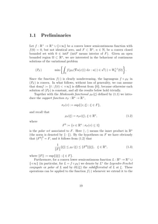
2.1 Preliminaries
Let us fix σ > 0 and consider two variational problems
min
Ω
[f(ρF ( u(x))) + σu(x)] dx : u(·) ∈ u0
(·) + W1,1
0 (Ω) (Pσ)
and
min
Ω
[f(ρF ( u(x))) − σu(x)] dx : u(·) ∈ u0
(·) + W1,1
0 (Ω) (P−σ)
Here f : R+
→ R+
∪ {+∞}, f(0) = 0, is a convex lower semicontinuous
function, F ⊂ Rn
is a convex closed bounded set with 0 ∈ intF, Ω ⊂ Rn
is
an arbitrary open bounded connected region and u0
(·) ∈ W1,1
(Ω). These are
our standing assumptions along with the chapter.
In what follows, as earlier, f∗
stands fot the Legendre-Fenchel transform
(conjugate) of the convex function f, and b > 0 is such that domf∗
= [0, b]
(or [0, b)). In particular, b can be +∞.
Let us introduce the (index) sets
Γ±
Ω := {γ = (x0, k) ∈ Ω × R : Ω ⊂ x0 ± b ·
n
σ
F0
} (2.3)
and the following Lipschitz continuous functions
ω+
γ (x) =
n
σ
f∗ σ
n
ρF0 (x − x0) + k, γ ∈ Γ+
Ω, (2.4)
ω−
γ (x) = −
n
σ
f∗ σ
n
ρF0 (x0 − x) + k, γ ∈ Γ−
Ω, (2.5)
defined on Ω. Further on we will naturally assume Ω ⊂ Rn
to be chosen
so small that Γ±
Ω = ∅. Sometimes it is convenient to consider only the case
when b = +∞ (equivalently, f(·) not affine on some semiline [b, +∞)).
The following result allows us to consider ω±
γ (·) as the possible candidates
to comparison functions for the problems (Pσ) and (P−σ).
54](https://image.slidesharecdn.com/tesefinal-160412170430/85/Tese-Final-net-55-320.jpg)
![Theorem 2.1.1. Let Ω ⊂ Rn
be an open bounded connected domain with
sufficiently regular boundary such that the Divergence Theorem holds (see,
e.g., [26]). Then the function ω+
γ (·) defined by (2.4) is the only solution to
(Pσ) with u0
(·) = ω+
γ (·). Similarly, the function ω−
γ (·) defined by (2.5) is the
only solution to (P−σ) with the same boundary condition, i.e., u0
(·) = ω−
γ (·).
The statement of Theorem follows immediately from Theorem 1 [13],
taking into account that the conjugate of the function ξ ∈ Rn
→ f(ρF (ξ))
coincides with f∗
(ρF0 (·)) and that the domain of (f ◦ ρF (·))∗
is the set bF0
or its interior.
Observe that although the Cellina’s result above holds for general func-
tional (with no symmetry assumption), we believe that such type symmetry
is rigorously needed for results below.
2.2 Comparison theorem
Here we obtain an auxiliary comparison result on minimizers of the varia-
tional problems (P±σ), which will be used further for proving local estimates
on minimizers as well as some local versions of SMP.
Theorem 2.2.1. Given ¯x ∈ Ω let us choose positive numbers α, β with α < β
such that the closure of the annulus A+
α,β(¯x) := {x ∈ Rn
: α < ρF0 (¯x−x) < β}
is contained in Ω. Assume that there exist M > 0 and a decreasing absolutely
continuous function R : [α, β] → R such that
M
rn−1
+
σ
n
r ∈ ∂f(|R (r)|) (2.6)
for a.e. r ∈ [α, β]. If a continuous minimizer ¯u(·) in (P−σ) satisfies the
inequality
¯u(x) ≥ R(ρF0 (¯x − x)) (2.7)
on the boundary ∂A+
α,β(¯x) then the same inequality takes place for all x ∈
A+
α,β(¯x).
Similarly, setting A−
α,β(¯x) := {x ∈ Rn
: α < ρF0 (x − ¯x) < β}, let us
assume that the closure A−
α,β(¯x) ⊂ Ω, and there exist a constant M > 0 and
an increasing absolutely continuous function R : [α, β] → R satisfying (2.6)
55](https://image.slidesharecdn.com/tesefinal-160412170430/85/Tese-Final-net-56-320.jpg)
![for a.e. r ∈ [α, β]. Then for an arbitrary continuous minimizer ¯u(·) in (Pσ)
validity of the inequality
¯u(x) ≤ R(ρF0 (x − ¯x)) (2.8)
on the boundary ∂A−
α,β(¯x) implies its validity for all x ∈ A−
α,β(¯x).
Proof. Let us prove the first part of Theorem. Denoting by
S(x) = R(ρF0 (¯x − x)),
we assume that the (open) set U = {x ∈ A+
α,β(¯x) : u(x) < S(x)} is nonempty.
Define the function ω(·) to be equal to max(¯u(x), S(x)) on A+
α,β(¯x) and to
¯u(x) elsewhere. Obviously, ω(·) is continuous and equals to S(x) on U. For
x ∈ ΩU instead ω(x) = ¯u(x). Now we show that ω(·) is a solution to (P−σ)
with u0
(x) = ω(x) = ¯u(x), x ∈ ∂Ω.
Since ¯u(·) is a minimizer in (P−σ), we have
0 ≥
Ω
{[f(ρF ( ¯u(x))) − σ¯u(x)] − [f(ρF ( (ω(x)))) − σω(x)]} dx =
=
U
[f(ρF ( ¯u(x))) − f(ρF ( S(x))) − σ(¯u(x) − S(x))] dx ≥
≥
U
[ p(x), (¯u(x) − S(x)) − σ(¯u(x) − S(x))] dx, (2.9)
where p(x) is a measurable selection of the mapping
x → ∂(f ◦ ρF )( S(x)).
We want to construct a selection p(·) such that the last integral in (2.9)
equals zero. To this end we define p(·) according to the differential properties
of S(x). Observe first that by (2.6) and monotonicity of the function R(·)
−R (r) ∈ ∂f∗ M
rn−1
+
σ
n
r (2.10)
for a.e. r ∈ [α, β]. Taking into account that the gradient ρF0 (¯x − x) exists
almost everywhere, we have
S(x) = −R (ρF0 (¯x − x)) ρF0 (¯x − x) (2.11)
56](https://image.slidesharecdn.com/tesefinal-160412170430/85/Tese-Final-net-57-320.jpg)
![for a.e. x ∈ U. Furthermore, the gradient ρF0 (¯x − x) belongs to ∂F (see
(1.4)) and, consequently,
ρF ( S(x)) = |R (ρF0 (¯x − x))| ∈ ∂f∗ M
ρn−1
F0 (¯x − x)
+
σ
n
ρF0 (¯x − x)
or, equivalently,
M
ρn−1
F0 (¯x − x)
+
σ
n
ρF0 (¯x − x) ∈ ∂f(ρF ( S(x)))
for a.e. x ∈ U. The subdifferential of the composed function f ◦ρF at S(x)
is equal to
∂f(ρF ( S(x)))∂ρF ( S(x)),
and by (1.4) the gradient S(x) is normal to F0
at ¯x−x
ρF 0 (¯x−x)
, or, in dual form,
¯x − x
ρF0 (¯x − x)
∈ NF
S(x)
ρF ( S(x))
∩ ∂F0
= ∂ρF ( S(x)).
So we can define the function
p(x) =
M
ρn−1
F0 (¯x − x)
+
σ
n
ρF0 (¯x − x)
¯x − x
ρF0 (¯x − x)
=
=
M(¯x − x)
ρn
F (¯x − x)
+
σ
n
(¯x − x),
which is a measurable selection of x → ∂(f ◦ ρF )( S(x)) on U. Then,
U
[ p(x), (¯u(x) − S(x)) − σ(¯u(x) − S(x))] dx =
=
U
σ
n
(¯x − x), (¯u(x) − S(x)) − σ(¯u(x) − S(x)) dx +
+
U
M(¯x − x)
ρn
F (¯x − x)
, (¯u(x) − S(x)) dx.
57](https://image.slidesharecdn.com/tesefinal-160412170430/85/Tese-Final-net-58-320.jpg)
) dx =
= −
σ
n A+
α,β(¯x)
div ([¯u(x) − ω(x)](x − ¯x)) dx =
=
σ
n ∂A+
α,β(¯x)
[¯u(x) − S(x)](¯x − x), n dx = 0, (2.12)
where n is the outward unit normal to the boundary (recall that ¯u(x) = ω(x)
outside A+
α,β(¯x)).
On the other hand, applying the polar coordinates r = x − ¯x and
ω = (x − ¯x)/ x − ¯x , and observing that for each ω, ω = 1, the equality
¯u(x) = S(x) holds on the boundary of the (open) linear set lω := {r ∈ (α, β) :
(r, ω) ∈ U}, we obtain as earlier (see Section 1.2)
U
M(¯x − x)
ρn
F0 (¯x − x)
, (¯u(x) − S(x)) dx =
= −M
ω =1
dω
ρn
F0 (−ω) lω
1
rn
< rω, (¯u(r, ω) − S(r, ω)) > rn−1
dr = 0.
Hence
U
[ p(x), (¯u(x) − S(x)) − σ(¯u(x) − S(x))] dx = 0, (2.13)
and, recalling (2.9), we have that ω(·) is a solution to (P−σ). It follows from
the same inequalities that
U
[f(ρF ( ¯u(x))) − f(ρF ( S(x))) − σ(¯u(x) − S(x))] dx = 0. (2.14)
Combining (2.13) and (2.14) we find
U
[f(ρF ( ¯u(x))) − f(ρF ( S(x))) − p(x), (¯u(x) − S(x)) ] dx = 0.
58](https://image.slidesharecdn.com/tesefinal-160412170430/85/Tese-Final-net-59-320.jpg)
![Taking into account the definition of the subdifferential of a convex function,
the integrand here is nonnegative, and we conclude that
f(ρF ( ¯u(x))) = f(ρF ( S(x))) + p(x), (¯u(x) − S(x))
a.e. on U. Notice that there is at most a countable family of disjoint open
intervals J1, J2, ... ⊂ [α, β] such that the real function f(·) is affine on each
Ji with a slope τi > 0, i = 1, 2, ... . Denoting by
Ei = {x :
M
ρn−1
F0 (¯x − x)
+
σ
n
ρF0 (¯x − x) = τi},
we have that for all x /∈
∞
i=1
Ei (the set of null measure) ∂f∗
(ρF0 (p(x))) is a
singleton. Thus ¯u(x) = S(x) for a.e. x ∈ U,which is a contradiction.
The second part of Theorem can be proved similarly with some obvious
changes. For instance, we define S(x) as the right-hand side of the inequality
(2.8) and ω(x) to be min(¯u(x), S(x)) on A−
α,β(¯x). Moreover, the respective
signs in (2.9), (2.10), (2.11) and (2.12) will be changed, and the final conclu-
sions remain valid.
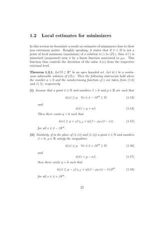
2.3 Local estimates of minimizers
In this section based on the comparison theorem from Section 2.2 we deduce
estimates of minimizers in the problems (Pσ) and (P−σ) in neighbourhoods
of points, which are (or not) points of local extremum. First, we prove that
if ¯x ∈ Ω is not a point of local maximum (minimum) of a solution ¯u(·) to
the problem (Pσ) (respectively, (P−σ)) then the deviation of ¯u(·) from the
extremal level can be controlled near ¯x by a solution ω±
γ to the respective
problem suggested by Theorem 2.1.1.
Theorem 2.3.1. Let Ω ⊂ Rn
, the gauge set F ⊂ Rn
and the function
f : R+
→ R+
∪ {+∞} satisfy our standing assumptions.
59](https://image.slidesharecdn.com/tesefinal-160412170430/85/Tese-Final-net-60-320.jpg)
![(i) Given a solution ¯u(·) to the problem (P−σ) let us assume that a point
¯x ∈ Ω is such that for some real k and β > 0
¯u(x) ≥ k ∀x ∈ ¯x − βF0
⊂ Ω, (2.15)
and
¯u(¯x) > k +
n
σ
f∗ σ
n
β . (2.16)
Then for all x ∈ ¯x − βF0
the inequality
¯u(x) ≥ k +
n
σ
f∗ σ
n
β − f∗ σ
n
ρF0 (¯x − x)
holds.
(ii) Similarly, if ¯u(·) is a solution to (Pσ) and a point ¯x ∈ Ω satisfies for
some k and β > 0 the conditions
¯u(x) ≤ k ∀x ∈ ¯x + βF0
⊂ Ω, (2.17)
and
¯u(¯x) < k −
n
σ
f∗ σ
n
β (2.18)
then
¯u(x) ≤ k −
n
σ
f∗ σ
n
β − f∗ σ
n
ρF0 (x − ¯x)
for all x ∈ ¯x + βF0
⊂ Ω.
Proof. (i) By continuity of ¯u(·) we find α ∈ (0, β) such that
¯u(x) > k +
n
σ
f∗ σ
n
β − f∗ σ
n
α (2.19)
for all x, ρF0 (¯x − x) ≤ α. It is obvious that the conjugate function f∗
(·) is
uniformly continuous on the segment I := [0, β + η] for some small η > 0.
So, fixed ε > 0 we can choose δ > 0 such that
|f∗
(t) − f∗
(s)| ≤
σε
2n
(2.20)
whenever t, s ∈ I with |t − s| ≤ δ. Combining (2.20) with (2.19) we have
that
¯u(x) > k − ε +
n
σ
f∗ σ
n
β + δ − f∗ σ
n
α + δ (2.21)
60](https://image.slidesharecdn.com/tesefinal-160412170430/85/Tese-Final-net-61-320.jpg)
![where γ = (x0, ¯u(x0)).
Similarly, let ¯u(·) be a continuous solution to (Pσ), x0 ∈ Ω be a point of
its local maximum, and δ > 0 be such that
¯u(x) ≤ ¯u(x0)
whenever x ∈ x0 − δF0
⊂ Ω. Then
¯u(x) ≥ ω−
γ (x)
for all x ∈ x0 − δ
F F0 +1
F0
with the same γ = (x0, ¯u(x0)).
Proof. Let us prove the first part of theorem. Assume, on the contrary, that
for some ¯x ∈ Ω with ρF0 (¯x − x0) ≤ δ
F F0 +1
the strict inequality
¯u(¯x) > k +
n
σ
f∗ σ
n
ρF0 (¯x − x0)
takes place with k := ¯u(x0). Let us choose ε > 0 so small that
( F F0
+ 1)ρF0 (¯x − x0) + ε F F0
< δ (2.27)
and
¯u(¯x) > k +
n
σ
f∗ σ
n
[ρF0 (¯x − x0) + ε] .
Seting β = ρF0 (¯x − x0) + ε we have
¯u(¯x) > k +
n
σ
f∗ σ
n
β . (2.28)
We claim now that ¯x − βF0
⊂ x0 + δF0
. Indeed, given y ∈ ¯x − βF0
by (1.3)
we have
ρF0 (y − ¯x) ≤ F F0
ρF0 (¯x − y) ≤ F F0
(ρF0 (¯x − x0) + ε),
and by (2.27)
ρF0 (y − x0) ≤ ρF0 (y − ¯x) + ρF0 (¯x − x0) < δ.
In particular, due to the condition (2.26) we have ¯u(x) ≥ k. Then by Theo-
rem 2.3.1 (see also the condition (2.28))
¯u(x) ≥ k +
n
σ
f∗ σ
n
β − f∗ σ
n
ρF0 (¯x − x)
63](https://image.slidesharecdn.com/tesefinal-160412170430/85/Tese-Final-net-64-320.jpg)
![Chapter 3
Rotationally invariant
lagrangeans with a nonlinear
term depending on u
In this Chapter we are interested in proving SMP for functionals which are
rotationally invariant with respect to the gradient and contain a nonlinear
additive term depending on the state variable. Namely, we consider the
minimization problem
min
Ω
[f( u(x) ) + g(u(x))] dx : u(·) ∈ u0
(·) + W1,1
0 (Ω) (Pg)
where f, g : R+
→ R+
are convex with f(0) = g(0) = 0.
Here we use the same notions of Convex Analysis as in the previous
chapters. Let us notice only that if a convex function f : R → R ∪ {+∞} is
differentiable at some point t then, in particular, the Fenchel identity
f(t) + f∗
(s) = ts ∀s ∈ ∂f(t)
can be written as
f∗
(f (t)) = tf (t) − f(t). (3.1)
If the functions f(·) and g(·) in (Pg) are sufficiently regular then we can
associate to (Pg) the Euler-Lagrange equation
div (f ◦ · )( u(x)) = g (u(x)),
65](https://image.slidesharecdn.com/tesefinal-160412170430/85/Tese-Final-net-66-320.jpg)
![which is a particular case of elliptic partial differential equations studied by
P. Pucci, J. Serrin and H. Zou (see [52, 54, 53]). In our terms the authors
assumed that
• f : R+
→ R+
, f(0) = 0, admits a strictly increasing continuous deriva-
tive on (0, +∞) such that limt→0+ f (t) = 0;
• g : R+
→ R+
has non-decreasing continuous derivative g (t), g (0) = 0,
on some interval [0, δ), δ > 0.
Under these standing hypotheses they gave the necessary and sufficient con-
ditions for validity of the SMP in the following form:
• either g(s) = 0 on [0, δ) or
• g(s) > 0 on (0, δ], and the (Riemann) improper integral
δ
0
ds
(f∗ ◦ f )−1(g(s))
(3.2)
diverges.
To obtain their results the authors used the comparison technique, where
the (auxiliary) comparison function, being itself a solution of the partial dif-
ferential equation, is constructed as a fixed point of some nonlinear compact
operator in the space of continuous functions.
We do not suppose the function g(·) to be continuously differentiable that
does not allow us to refer directly to the results obtained in the context of
Partial Differential Equations. However, we try to adapt the technique by
P. Pucci and J. Serrin to the case of the multivalued subdifferential. In par-
ticular, we are lead to consider a set-valued upper semicontinuous operator
in the functional space and to prove a parametrized version of the Kakutani
theorem. It turns out that a fixed point of the so constructed multifunction
satisfies all the properties announced in the works by P. Pucci and J. Ser-
rin and can be used as a comparison function in the variational technique
developed by A. Cellina for the functionals depending only on the gradient
(see Chapter 1). Thus, in the last section of this chapter we conclude the
proof of the variational SMP for the problem (Pg). It is interesting to ob-
serve that despite of the essentially multivalued character of the proof (that,
in our opinion, can not be avoided), the final sufficient condition forvalidity
66](https://image.slidesharecdn.com/tesefinal-160412170430/85/Tese-Final-net-67-320.jpg)
![of the SMP is obtained, exactly, in the form above (including divergence of
the integral (3.2)) by exploiting the fact that the convex function g(·) admits
derivative at almost each point.
3.1 Construction of the auxiliary operator
Similarly as in the works by P. Pucci and J. Serrin ([53, 54]) we search a
comparison function ω : C([0, β − α], R) → R such as
ω(t) = m −
β−α
t
(f )−1 1
(β − s)n−1
×
× λ −
β−α
s
(β − τ)n−1
p(τ) dτ ds, (3.3)
where p(·) is a measurable selection of t → ∂g(ω(t)) and λ > 0 is such that
ω(0) = 0. In order to prove the existence of such a function we make some
constructions as follows.
Let us denote by F the class of all strictly convex functions f : R+
→ R+
,
f(0) = 0, admitting continuous derivative f (·) on (0, +∞) with limt→0+ f (t) =
0, and by G the family of functions g : R+
→ R+
, g(0) = 0, which are convex
on some interval [0, δ), δ > 0, such that ∂g(0) = {0}.
For our convenience we extend the functions f (·) and g(·) to the whole
real line by setting f (s) = −f (−s) and g(s) = 0 for s < 0. Also choosing an
arbitrary m ∈ (0, δ) (the exact sense of this constant will be clarified later)
we redefine g(z) for z ≥ m by affine way.
Choose also α, β with 0 < α < β and set ¯p := sup{z : z ∈ ∂g(u), u ∈
[0, m]} and
¯λ := βn−1
f
σm
β − α
+ ¯p(β − α) . (3.4)
Given ω(·) ∈ C([0, β − α], R) and σ ∈ [0, 1] let us consider the multifunction
Pω,σ : [0, ¯λ] → R defined by
Pω,σ(λ) = σm −
β−α
0
(f )−1
((β − s)1−n
[λ −
−σ
β−α
s
(β − τ)n−1
∂g(ω(τ)) dτ]) ds. (3.5)
67](https://image.slidesharecdn.com/tesefinal-160412170430/85/Tese-Final-net-68-320.jpg)
![We claim that Pω,σ(·) is upper semicontinuous. Indeed, for each λ ∈ [0, ¯λ]
and u ∈ Pω,σ(λ) we have
u = σm −
β−α
0
(f )−1
((β − s)1−n
[λ −
−σ
β−α
s
(β − τ)n−1
p(τ) dτ]) ds (3.6)
for some measurable selection p(·) of t → ∂g(ω(t)) on [0, β − α]. By (3.4)
and monotonicity of the derivative f (·), on one hand, the number (3.6) is
not smaller than
−
β−α
0
(f )−1 βn−1
(β − s)n−1
f
m
β − α
+ ¯p(β − α) ds ≥
≥ −
β−α
0
(f )−1 β
α
n−1
f
m
β − α
+ ¯p(β − α) ds =
= −(β − α)(f )−1 β
α
n−1
f
m
β − α
+ ¯p(β − α) ,
while, on the other hand,
u ≤ σm −
β−α
0
(f )−1
−
β
α
n−1
¯p(β − α) ds =
= σm + (β − α)(f )−1 β
α
n−1
¯p(β − α) .
Therefore the values of Pω,σ(·) are contained in [C1, C2] for some real C1, C2,
and we need to prove only that Pω,σ(·) has closed graph. Consider a sequence
of elements (λk, vk) ∈ graph Pω,σ that converges to some (λ, v) ∈ [0, ¯λ] ×
[C1, C2]. We can represent
vk = σm −
β−α
0
(f )−1 1
(β − α)n−1
×
× λk − σ
β−α
t
(β − τ)n−1
pk(τ) dτ ds
for some measurable selection pk(·) of t → ∂g(ω(t)), k = 1, 2, .... It follows
from the upper semicontinuity of the latter multifunction that the sequence
68](https://image.slidesharecdn.com/tesefinal-160412170430/85/Tese-Final-net-69-320.jpg)
![(pk(·))k is bounded and by the Dunford - Pettis theorem we may assume
without loss of generality that it converges weakly to some p(t) ∈ ∂g(ω(t))
(the subdifferential admits convex values). Then for each t ∈ [0, β − α] the
integrals
β−α
t
(β − τ)n−1
pk(τ) dτ
converge to
β−α
t
(β − τ)n−1
p(τ) dτ,
and using continuity of the functions (f )−1
(·), Lebesgue dominated conver-
gence theorem and unicity of the limit we conclude that
v = σm −
β−α
0
(f )−1 1
(β − α)n−1
λ − σ
β−α
t
(β − τ)n−1
p(τ) dτ ds,
i.e., (λ, v) ∈ graph Pω,σ. Hence Pω,σ(·) is upper semicontinuous.
Now we prove existence of c ∈ [0, ¯λ] such that 0 ∈ Pω,σ(c). Let us start
by observing that Pω,σ(0) ⊂ [0, +∞) and Pω,σ(¯λ) ⊂ (−∞, 0]. Indeed, let
z1 ∈ Pω,σ(0). This means that for some measurable selection p1(t) ∈ ∂g(ω(t))
accordingly to our convention
z1 = σm −
β−α
0
(f )−1 −σ
(β − s)n−1
×
×
β−α
s
(β − τ)n−1
p1(τ) dτ ds ≥ σm ≥ 0,
Similarly, if z2 ∈ P(¯λ) then there exists a measurable selection p2(t) ∈
∂g(ω(t)) with
z2 = σm −
β−α
0
(f )−1
((β − s)1−n
)[βn−1
f (σm/(β − α))+
+¯pβn−1
(β − α) − σ
β−α
s
(β − τ)n−1
p2(τ) dτ]) ds ≤
≤ σm −
β−α
0
(f )−1
f
σm
β − α
ds = 0.
69](https://image.slidesharecdn.com/tesefinal-160412170430/85/Tese-Final-net-70-320.jpg)
![Let us choose a sequence of continuous approximate selections (fk)k of
the mapping λ → Pω,σ(λ), i.e., such that
graph fk ⊂ graph Pω,σ +
1
k
¯B, (3.7)
k = 1, 2, ... (see [4]). These selections, clearly can be chosen passing through
some fixed points of graph Pω,σ, say fk(0) = u0 ≥ 0 and fk(¯λ) = u¯λ ≤
0. By Bolzano theorem there exists a sequence (ck)k in (0, ¯λ) such that
fk(ck) = 0. Without loss of generality we assume that ck converges to some
c ∈ [0, ¯λ]. Therefore, by (3.7) there exist sequences (λk)k ⊂ [0, ¯λ] and (uk)k,
uk ∈ Pω,σ(λk) such that |uk| + |ck − λk| → 0, or, in other words, λk → c and
uk → 0 as k → ∞. Consequently, 0 ∈ Pω,σ(c) as required.
Let us consider now the set of all zeros
Λ(ω, σ) := {c ∈ [0, ¯λ] : 0 ∈ Pω,σ(c)}
and show that the mapping (ω, σ) → Λ(ω, σ) defined on C([0, β−α], R)×[0, 1]
has closed graph. To this end, we choose sequences (ωk(·))k ⊂ C([0, β−α], R),
(σk)k ⊂ [0, 1] and (ck)k ⊂ [0, ¯λ] such that
σkm =
β−α
0
(f )−1 1
(β − s)n−1
×
× ck − σk
β−α
s
(β − τ)n−1
pk(τ) dτ ds (3.8)
for some measurable selections pk(t) ∈ ∂g(ωk(t)), t ∈ [0, β − α], converging,
respectively, to a function ω(·) ∈ C([0, β − α], R), to σ ∈ [0, 1] and to some
c ∈ [0, ¯λ]. Due to the upper semicontinuity of the subdifferential, given
k = 1, 2, .... we choose ik ≥ 1 such that
∂g(ωik
(t)) ⊂ ∂g(ω(t)) +
1
k
¯B (3.9)
for all t ∈ [0, β − α]. Notice that ik does not depend on t by the uniform
convergence of functions. It follows from (3.9) that there exist measurable
selections qik
(t) ∈ ∂g(ω(t)) such that pik
(t)−qik
(t) → 0 as k → +∞ uniformly
in t ∈ [0, β − α]. Choosing if necessary a subsequence from (qik
(·))k we may
suppose that (qik
(·))k and, consequently, (pik
(·))k converges weakly to some
measurable selection p(t) ∈ ∂g(ω(t)). This implies the weak convergence of
70](https://image.slidesharecdn.com/tesefinal-160412170430/85/Tese-Final-net-71-320.jpg)
![the integrals
β−α
s
(β − τ)n−1
pik
(τ) dτ for each s ∈ [0, β − α]. Passing now to
the limit in the equality (3.8) we conclude that c ∈ Λ(ω, σ).
Let us denote by H(ω, σ) the set of continuous mappings
t → σm −
β−α
t
(f )−1 1
(β − s)n−1
×
× λ − σ
β−α
t
(β − τ)n−1
p(τ) dτ ds (3.10)
for all measurable selections p(t) ∈ ∂g(ω(t)) and all λ ∈ Λ(ω, σ). In the next
section we prove existence of a function satisfying (3.3) through fixed points
of the one-parametric family of the multivalued mappings ω → H(ω, σ).
3.2 Existence of a fixed point
We preface the proof of existence theorem with several lemmas.
Lemma 3.2.1. The multivalued mapping
H : C([0, β − α], R) × [0, 1] → C([0, β − α], R)
defined above (see (3.10)) has closed graph.
Proof. Let (ωk)k ⊂ C([0, β−α], R), (σk)k ⊂ [0, 1] and (vk)k ⊂ C([0, β−α], R),
vk(·) ∈ H(ωk, σk), k = 1, 2, ..., be sequences converging, respectively, to ω(·),
to σ ∈ [0, 1] and to v(·). Representing each function vk(·) as
vk(t) = σm −
β−α
t
(f )−1 1
(β − s)n−1
×
× λk − σk
β−α
t
(β − τ)n−1
pk(τ) dτ ds (3.11)
for some λk ∈ Λ(ωk, σk) and some measurable selection pk(t) ∈ ∂g(ωk(t)),
t ∈ [0, β−α], we assume without loss of generality that λk → λ ∈ Λ(ω, σ) (see
Section 3.1) and that the sequence (pk)k converges weakly to a measurable
71](https://image.slidesharecdn.com/tesefinal-160412170430/85/Tese-Final-net-72-320.jpg)
![function p(t) ∈ ∂g(ω(t)), t ∈ [0, β − α]. Passing now to the (pointwise) limit
in (3.11), we conclude that
v(t) = σm −
β−α
t
(f )−1 1
(β − s)n−1
λ − σ
β−α
t
(β − τ)n−1
p(τ) dτ ds,
t ∈ [0, β − α]. Thus, (ω(·), σ, v(·)) belongs to graph H, and the statement is
proved.
Lemma 3.2.2. Given C > 0 there exists a compact set KC ⊂ C([0, β−α], R)
such that H(ω, σ) ⊂ KC for all ω(·) ∈ C([0, β − α], R) with w(t) ≤ C,
t ∈ [0, β − α], and for all σ ∈ [0, 1].
Proof. Since the subdifferential ∂g(·) is bounded on the ball C ¯B, the set of
functions t →
β−α
t
(β − τ)n−1
p(τ) dτ for all p(t) ∈ ∂g(ω(t)), ω(t) ≤ C,
t ∈ [0, β − α], is relatively compact in C([0, β − α], R). Furthermore, since
the function (f )−1
is continuous, the expression under the first integral in
(3.10) is contained in some ball RC
¯B. Therefore, H(ω, σ) ⊂ KC for all
ω(·) ∈ C([0, β − α], R) with ω(t) ≤ C, where
KC := {x(·) ∈ C1
([0, β − α], R) : ˙x(t) ≤ RC ∀t ∈ [0, β − α]},
is relatively compact in C([0, β − α], R) by Ascoli-Arzel`a theorem.
Lemma 3.2.3. The set
A := {(ω, σ) ∈ C([0, β − α], R) × [0, 1] : ω ∈ H(ω, σ)}.
is nonempty and bounded.
Proof. Nonemptiness of A is obvious ((0, 0) ∈ A ). In order to show the
boundedness let us represent each ω(·) with ω ∈ H(ω, σ) in the form
ω(t) = σm −
β−α
t
(f )−1 1
(β − s)n−1
×
× λ − σ
β−α
s
(β − τ)n−1
p(τ) dτ ds, (3.12)
with some λ ∈ Λ(ω, σ) ⊂ [0, ¯λ], and some measurable selection p(t) ∈
∂g(ω(t)). Since the subdifferential ∂g(z) is bounded on [0, m] and single-
valued for z ≥ m, we immediately obtain boundedness of the right-hand side
of (3.12).
72](https://image.slidesharecdn.com/tesefinal-160412170430/85/Tese-Final-net-73-320.jpg)
![Now we are ready to prove a fixed point theorem. For this we adopt the
Leray-Schauder theorem (see, e.g., [36]) to multivalued operators by using
one of the versions of Kakutani theorem, proved by Bohnenblust and Karlin
(see, e.g., [5]).
Theorem 3.2.1. The multivalued mapping ω → H(ω, 1) has a fixed point
ω(·) such that ω(0) = 0.
Proof. In accordance with Lemma 3.2.3, there exists M > 0 such that ω ≤
M whenever (ω, σ) ∈ A, σ ∈ [0, 1]. Consider the linear space
B = {ω ∈ C([0, β − α], R) : ω(0) = 0}
and given ε > 0 define the multivalued operator Fε : B → B,
Fε(ω) =
H Mω
M−ε
, 1 ∩ B if ω ≤ M − ε,
H Mω
ω
, M− ω
ε
∩ B if M − ε < ω < M,
{0} if ω ≥ M.
Due to upper semicontinuity of (ω, σ) → H(ω, σ), by the construction it
follows that the set-valued mapping Fε : B → B is upper semicontinuous as
well. Moreover, it admits nonempty values due to the definition of Λ(ω, σ).
The values of Fε(·) are, obviously, closed and by Lemma 3.2.2 contained
in the compact set KM . Then, applying Bohnenblust-Karlin theorem (see
[5]) we find a fixed point ωε(·) ∈ B, ωε(·) ∈ Fε(ωε).
Setting ε = 1
k
, k = 1, 2, ..., and denoting by
σk =
1 if ω1
k
≤ M − 1
k
,
k(M − ω 1
m
) if M − ε < ω1
k
< M,
0 if ω1
k
≥ M,
we observe first that
ω1
k
∈ H(ω1
k
, σk) (3.13)
for each k = 1, 2, ..., and, consequently, (ω1
k
, σk) ∈ A. Since ω1
k
(·) ∈ KM
and σk ∈ [0, 1], without loss of generality we can assume that the sequence
(ω1
k
)k converges uniformly to some ω(·) ∈ B, ω(0) = 0, and σk → σ ∈ [0, 1].
Passing to the limit in (3.13) as k → ∞, by closedness of graph H we obtain
ω ∈ H(ω, σ).
73](https://image.slidesharecdn.com/tesefinal-160412170430/85/Tese-Final-net-74-320.jpg)
![Let us show finally that σ = 1. Assuming σ < 1, we have σk < 1 for all
k ≥ 1 large enough and consequently ω1
k
> M − 1
k
. Passing to the limit we
obtain ω ≥ M, contradicting the choice of M > 0. Theorem is proved.
Thus, there exist λ ∈ Λ(ω, 1) ⊂ [0, ¯λ] and a measurable selection p(·) of
the mapping t → ∂g(ω(t)) on [0, β − α], such that
ω(t) = m −
β−α
t
(f )−1 1
(β − s)n−1
×
× λ −
β−α
s
(β − τ)n−1
p(τ) dτ ds
and ω(0) = 0.
3.3 Properties of the comparison function
In the previous section we proved existence of a function ω(·) ∈ C([0, β −
α], R) such that for some measurable selection p(t) ∈ ∂g(ω(t)) the equality
(3.3) holds. Fixed such a function we study now some of its properties.
Lemma 3.3.1. The function ω(·) is continuously differentiable on [0, β − α]
and
(a) ω(t) ≥ 0 ∀t ∈ [0, β − α];
(b) ω (t) ≥ 0 ∀t ∈ [0, β − α];
(c) there exists ¯t ∈ [0, β − α) such that ω(t) ≡ 0 on [0, ¯t] and ω(t) > 0,
ω (t) > 0 on (¯t, β − α].
Proof. The continuous differentiability of ω(·) follows from (3.3) and conti-
nuity of (f )−1
((f )−1
is continuous since f is continuous and strictly in-
creasing).
If the statement (a) is not true then, taking into account that ω(0) = 0
and ω(β −α) = m > 0, one can choose two different points t0, t1 ∈ [0, β −α),
74](https://image.slidesharecdn.com/tesefinal-160412170430/85/Tese-Final-net-75-320.jpg)
![t0 < t1, such that ω(t0) = ω(t1) = 0 and ω(t) < 0 for t ∈ (t0, t1). It follows
from (3.3) that
[(β − t)n−1
f (ω (t))] = (β − t)n−1
p(t) (3.14)
for all t ∈ [0, β − α]. Multiplying both sides of (3.14) by ω(t) and integrating
by parts on [t0, t1] yields
t1
t0
(β − t)n−1
f (ω (t))ω (t) dt = −
t1
t0
(β − t)n−1
p(t)ω(t) dt.
Since p(t) ∈ ∂g(ω(t)), ω(t) < 0 for t ∈ [t0, t1], and by the convention g(s) = 0
for s ≤ 0, we have p(t) = 0 for all t ∈ [t0, t1]. Hence,
t1
t0
(β − t)n−1
f (ω (t))ω (t) dt = 0. (3.15)
Recall that xf (x) > 0 for all x = 0. Then the equality (3.15) means that
ω (t) ≡ 0 on [t0, t1], and, hence, ω(t) ≡ 0 because ω(t0) = ω(t1) = 0, which
is a contradiction.
In order to prove items (b) and (c), let us define the set
J = {t ∈ (0, β − α) : ω (t) > 0},
which is nonempty (because ω(0) = 0 and ω(β − α) = m > 0), and open by
continuity of the derivative ω (·).
Set ¯t = infJ ∈ [0, β − α). Then ω(t) =
t
¯0
ω (s) ds ≤ 0 for each t ∈ [0, ¯t].
Consequently, by (a) we conclude that ω ≡ 0 on [0, ¯t]. Furthermore, for each
t ∈ (¯t, β −α] there exists ˆt, ¯t < ˆt < t such that ˆt ∈ J. Then, by monotonicity
of the function s → (f )−1
(s) we have
ω (t) = (f )−1 1
(β − t)n−1
λ −
β−α
t
(β − τ)n−1
p(τ) dτ ≥
≥ (f )−1 1
(β − ˆt)n−1
λ −
β−α
ˆt
(β − τ)n−1
p(τ) dτ = ω (ˆt) > 0.
Thus, ω (t) > 0 and
ω(t) =
t
¯t
ω (s) ds > 0
for all t ∈ (¯t, β − α].
75](https://image.slidesharecdn.com/tesefinal-160412170430/85/Tese-Final-net-76-320.jpg)
![The important step in proving the validity of SMP consists in the estab-
lishment of a connection between properties of the function ω(·) and diver-
gence of the improper integral (3.2). Namely, through the following estimates
we prove that this divergence implies that ω (0) > 0. In other words, in terms
of the previous lemma ˆt = 0.
Lemma 3.3.2. Assuming that ω (0) = 0, the inequality
f (ω (t)) ≤
p(t)
(β − t)n−1
βn
n
−
(β − t)n
n
(3.16)
holds for t ∈ [0, β − α].
Proof. By integrating the equality (3.14) (which is equivalent to the repre-
sentation of ω(·), see (3.3)) on a segment [τ, t], 0 ≤ τ ≤ t ≤ β − α, we
have
(β − t)n−1
f (ω (t)) − (β − τ)n−1
f (ω (τ)) =
t
τ
(β − s)n−1
p(s) ds.
Letting τ → 0+
, due to monotonicity of the function ω(·) and of the subd-
ifferential ∂g(·), taking into account that f (·) and ω (·) are continuous and
ω (0) = 0, we obtain that
(β − t)n−1
f (ω (t)) ≤ p(t)
t
0
(β − s)n−1
ds,
and the estimate (3.16) follows.
In the lemma above we proved an estimate on f along with ω (·). Now
we treat the same property for the composed function f∗
◦ f .
Lemma 3.3.3. Assume that ω(·) is such as in Lemma 3.3.2 . Then,
f∗
(f (ω (t))) ≤ L(t)
t
0
p(s)ω (s) ds
for all t ∈ [0, β − α] where
L(t) := 1 +
n − 1
n
β
β − t
n
− 1 . (3.17)
76](https://image.slidesharecdn.com/tesefinal-160412170430/85/Tese-Final-net-77-320.jpg)
![Proof. By (3.1) we find
f∗
(f (ω (t))) = ω (t)f (ω (t)) − f(ω (t)) =
= ω (t)f (ω (t)) −
ω (t)
0
f (s) ds, (3.18)
t ∈ [0, β − α]. Integrating (3.18) by parts, we obtain that
f∗
(f (ω (t))) =
ω (t)
0
s df (s). (3.19)
Since f (·) is strictly increasing, we can make the change of variables y = f (s)
in the Stieltjes integral (3.19) and arrive at the formula
f∗
(f (ω (t))) =
f (ω (t))
0
(f )−1
(y) dy. (3.20)
It follows from (3.20) that the function f∗
◦ (f ◦ ω ) is almost everywhere
differentiable on [0, β − α], and
[f∗
(f (ω (t)))] = ω (t)[f (ω (t))] (3.21)
for a.e. t ∈ [0, β − α]. Derivating in the left-hand side we can rewrite the
equality (3.14) in the form
(f (ω (t)) =
n − 1
β − t
f (ω (t)) + p(t).
Then, substituting to (3.21) and integrating on the segment [0, t] we have
f∗
(f (ω (t))) =
t
0
n − 1
β − s
f (ω (s))ω (s) ds +
t
0
p(s)ω (s) ds.
Hence, applying the estimate (3.16), we obtain
f∗
(f (ω (t))) ≤
t
0
n − 1
β − s
·
p(s)
(β − s)n−1
×
×
βn
n
−
(β − s)n
n
ω (s) + p(s)ω (s) ds =
=
t
0
1 +
n − 1
(β − s)n
βn
n
−
(β − s)n
n
p(s)ω (s) ds ≤
≤ L(t)
t
0
p(s)ω (s) ds,
and Lemma is proved.
77](https://image.slidesharecdn.com/tesefinal-160412170430/85/Tese-Final-net-78-320.jpg)
![We are ready now to establish the main property of the function ω(·),
which will be used in the sequel.
Theorem 3.3.1. Assume that g ∈ G is strictly increasing. If ω (0) = 0 then
for each δ > 0 the integral
δ
0
ds
(f∗ ◦ f )−1(g(s))
converges.
Proof. By Lemma 3.3.1 there exists ¯t ∈ [0, β − α) such that ω(t) = 0 for
t ∈ [0, ¯t] while ω(t) > 0 in (¯t, β − α). By the monotonicity of f and f∗
the
limit (finite or infinite)
D := limt→+∞f∗
(f (t))
exists. Observe that the derivative f (·) can be upper bounded by a constant
µ ∈ domf∗
, and the latter domain not necessarily coincides with R. Due to
this fact the limit D can be finite as well. Let us fix now δ > 0 and t1 and
t2, 0 < ¯t < t1 < t2 < β − α such that
ω(t1)L(t2) < δ
and
ω(t1)L(t2)
0
p(ω−1
(y)) dy < D,
where p(·) is the measurable selection of ∂g(ω(·)) associated to ω(·), and L(·)
is defined by (3.17).
By Lemma 3.3.3,
f∗
(f (ω (t))) ≤ L(t)
t
0
p(s)ω (s) ds ≤
≤ L(t2)
t
¯t
p(s)ω (s) ds (3.22)
for all t ∈ [¯t, t2] (notice that the function L(·) is nondecreasing). Taking into
account the strict monotonicity of the function ω(·) on [¯t, t2] we can apply
to the integral in (3.22) the change of variables y = L(t2)ω(s) and obtain
t
¯t
p(s)ω (s) ds =
1
L(t2)
L(t2)ω(t)
0
p ω−1 y
L(t2)
dy. (3.23)
78](https://image.slidesharecdn.com/tesefinal-160412170430/85/Tese-Final-net-79-320.jpg)
![Theorem 3.4.1. If Ω = Aα,β(x0
) and ω(·) ∈ C([0, β − α], R) satisfies the
equality (3.3) for some (fixed) measurable p(t) ∈ [0, β − α] then the function
V : Ω → R, V (x) = ω(β − x − x0
) is a solution to (Pg) with u0
(x) = V (x).
Proof. Denoting by q(x) := p(β − x − x0
) and taking arbitrary u(·) ∈
V (·) + W1,1
0 (Ω), we sucessively obtain
Ω
(f( u(x) ) + g(u(x)) − [f( V (x) ) + g(V (x))]) dx ≥
≥
Ω
[ (f ◦ · )( V (x)), u(x) − V (x) +
+ q(x)(u(x) − V (x))] dx =
Ω
[f ( V (x) ) −(x − x0
)/ x − x0
,
u(x) − V (x) + q(x)(u(x) − V (x))] dx. (3.27)
Here we used the definition of the subdifferential ∂g(·) and convexity of the
function f.
Let us recall the definition of ω(·) (see (3.3)), which can be written in the
form
f (ω (t)) =
1
(β − t)n−1
λ −
β−α
t
(β − τ)n−1
p(τ) dτ , (3.28)
or
f (−v (r)) =
1
rn−1
λ +
α
r
sn−1
p(β − s) ds , (3.29)
where v(r) := ω(β − r), α ≤ r ≤ β. Pass now to the polar coordinates r =
x − x0
and θ = x−x0
x−x0 in (3.27), taking into account that V (x) = v (r)θ
and V (x) = −v (r). So, we can represent the last integral in (3.27) as
θ =1
dθ
β
α
−f (−v (r))
d
dr
(u(θ, r) − v(r)) rn−1
dr +
+
β
α
[p(β − r)(u(θ, r) − v(r))] rn−1
dr . (3.30)
Further, substituting the value of f (−v (r)) from (3.29) and integrating by
parts the first integral in (3.30) with respect to the variable r ∈ [α, β], we
80](https://image.slidesharecdn.com/tesefinal-160412170430/85/Tese-Final-net-81-320.jpg)
![reduce (3.30) to
θ =1
−
β
α
((u(r, θ) − v(r))rn−1
p(β − r) dr+
+
β
α
((u(r, θ) − v(r))rn−1
p(β − r) dr dθ = 0. (3.31)
We used here the fact that the functions u(·) and v(·) admit the same values
on the boundary of Ω. Combining (3.31) and (3.27) we conclude
Ω
[f( V (x) ) + g(V (x))] dx ≤
Ω
[f( u(x) ) + g(u(x))] dx,
and Theorem is proved.
We know from the results of the previous section that ω(t) > 0 on (0, β−α]
and ω (t) > 0 on [0, β − α] under the assumption (3.2) . In order to prove
the Srong Maximum Principle we need the following comparison result.
Theorem 3.4.2. Let Ω ⊂ Rn
be an open bounded connected region, x0
∈ Ω
and α, β, 0 < α < β, be such that Aα,β(x0
) ⊂ Ω, and ω(·) be a continuous
function defined by (3.3). Set v(r) := ω(β − r), r ∈ [α, β], and suppose that
u(·) is a continuous solution of (Pg) with
u(x) ≥ v( x − x0
) ∀x ∈ ∂Aα,β(x0
).
Then the same inequality holds for all x ∈ Aα,β(x0
).
Proof. Let us denote V (x) = v( x − x0
) and assume, on contrary, that the
(open) set
E−
= {x ∈ Aα,β(x0
) : u(x) < V (x)}
is non empty. Define the function η−
(x) equal to
min{u − V, 0} =
u(x) − V (x) if x ∈ E−
,
0 if x ∈ Aα,β(x0
) E−
,
and to zero on Ω Aα,β(x0
). Clearly, η−
(·) ∈ W1,1
0 (Ω) is continuous,
(u − η−
)(x) =
V (x) if x ∈ E−
,
u(x) if x ∈ Ω E−
,
(3.32)
81](https://image.slidesharecdn.com/tesefinal-160412170430/85/Tese-Final-net-82-320.jpg)
![and (see [41])
(u − η−
)(x) =
V (x) for a.e. x ∈ E−
,
u(x) for a.e. x ∈ Ω E−
.
(3.33)
Since u(·) is a solution of (Pg), it follows from (3.32) and (3.33) that
0 ≥
Ω
(f( u(x) ) + g(u(x)) −
− [f( (u − η−
)(x) ) + g((u − η−
)(x))]) dx =
=
E−
[f( u(x) ) − f( V (x) ) + g(u(x)) − g(V (x))] dx ≥
≥
E−
[ (f ◦ · )( V (x)), u(x) − V (x) + q(x)(u(x) − V (x))] dx =
=
E−
[f ( V (x) ) −(x − x0
)/ x − x0
, u(x) − V (x) +
+ q(x)(u(x) − V (x))] dx, (3.34)
where q(x) := p(β − x − x0
), and p(t) as usual is the measurable selection
of t → ∂g(ω(t)), associated to ω(·). Introducing the polar coordinates r =
x−x0
and θ = x−x0
x−x0 similarly as in the proof of Theorem 3.4.1 we reduce
the last integral in (3.34) to
θ =1 lθ
f (−v (r))
d
dr
(u(θ, r) − v(r)) rn−1
dr+
+
lθ
p(β − r)(u(θ, r) − v(r))rn−1
dr dθ, (3.35)
where lθ := {r ∈ (α, β) : (r, θ) ∈ E−
}.
Recalling (3.29), integrating (3.35) by parts and taking into account that
the functions u(θ, r) and v(r) coincide on the boundary of the linear set lθ,
θ ∈ [α, β], similarly as in the proof of Theorem 3.4.1, we we deduce from
(3.34) that
E−
[f( u(x) ) − f( V (x) ) + g(u(x)) − g(V (x))] dx = 0. (3.36)
It follows also (see (3.34)) that
E−
[ (f ◦ · )( V (x)), u(x) − V (x) +
+ q(x)(u(x) − V (x))] dx = 0. (3.37)
82](https://image.slidesharecdn.com/tesefinal-160412170430/85/Tese-Final-net-83-320.jpg)
![On the other hand, the integral
E−
[f( u(x) ) − f( V (x) ) + q(x)(u(x) − V (x))] dx
is contained between the integrals (3.36) and (3.37), and so it is equal to zero
as well. Hence,
E−
[f( u(x) ) − f( V (x) ) −
− (f ◦ · )( V (x)), u(x) − V (x) dx = 0. (3.38)
By convexity, the integrand in (3.38) is nonnegative for a.e. x ∈ E−
and we
have the pointwise equality
f( u(x) ) = f( V (x) ) +
+ (f ◦ · )( V (x)), u(x) − V (x)
for a.e. x ∈ E−
. In other words, ( u(x), f( u(x) )) belongs to the same
face of the epigraph of the convex function z → f( z ) as ( V (x), f( V (x) )).
Since f is strictly convex, we conclude that u(x) = V (x) a.e. in E−
, i.e.
η−
= 0 on Ω, which is a contradiction.
Finally, the following theorem gives sufficient conditions for the validity
of the Strong Maximum Principle.
Theorem 3.4.3. In addition to our standing assumptions let us suppose that
either g(s) = 0, s ∈ [0, δ], for some δ > 0, or g(s) > 0 near zero and for
some δ > 0 the Riemann improper integral (3.2) diverges. Then the Strong
Maximum Principle holds for the problem (Pg).
Proof. In the first case (g(s) = 0 ∀s ∈ (0, δ]) the Strong Maximum Principle
is proved in [16].
Let us consider the second hypothesis, i.e.,
δ
0
ds
(f∗ ◦ f )−1(g(s))
= +∞.
Let Ω ⊂ Rn
be any open bounded connected domain and u(·) be a continuous
nonnegative solution of (Pg). Suppose that both sets
E = {x ∈ Ω : u(x) = 0} and Ω E = {x ∈ Ω : u(x) > 0}
83](https://image.slidesharecdn.com/tesefinal-160412170430/85/Tese-Final-net-84-320.jpg)
![are nonempty. Due to connectedness of Ω there exists x∗
∈ E ∩ Ω E.
Choose β > 0 such that the ball ¯B2β(x∗
) ⊂ Ω, and let x0
∈ Ω E be
such that x∗
− x0
< β. From continuity of u(·) one can find m ∈ (0, δ)
and α ∈ (0, x∗
− x0
) such that u(x) ≥ m on ¯Bα(x0
). We associate to the
numbers α, β and m a function ω(·) ∈ C([0, β−α], R) studied in the previous
sections, which is defined by the formula (3.3) with some measurable selection
p(t) ∈ ∂g(ω(t)), and consider the annulus
Aα,β(x0
) := {x ∈ Rn
: α < x − x0
< β}.
Let us set v(r) = ω(β − r), r ∈ [α, β], and apply the comparison theorem.
Namely, by the choice of the constants m and α we obviously have u(x) ≥
v( x − x0 ) whenever x − x0 is equal to α or to β. By Theorem 2.4.2
the same inequality holds also inside the annulus Aα,β(x0
). In particular,
u(x∗
) ≥ v( x∗
−x0 ). But by Lemma 2.3.1 and Theorem 2.3.1 the derivative
v (r) is negative on [α, β], i.e., the function v(·) is strictly decreasing. Then
u(x∗
) ≥ v( x∗
− x0 ) > v(β) = 0, which is a contradiction.
Example 5. Consider the problem of minimizing the integral functional
Ω
[ u(x) p
+ (u(x))p
] dx
with p > 1. Here f(ξ) = ξp
for ξ > 0, its derivative f (ξ) = pξp−1
, and
f∗
(v) = v
v
p
1
p−1
−
v
p
p
p−1
.
Thus,
(f∗
◦ f )(t) = (p − 1)tp
;
(f∗
◦ f )−1
(t) =
t
p − 1
1
p
,
and
δ
0
ds
(f∗ ◦ f )−1(g(s))
=
δ
0
ds
sp
p−1
1
p
= +∞.
So, the Strong Maximum Principle holds by the above theorem.
84](https://image.slidesharecdn.com/tesefinal-160412170430/85/Tese-Final-net-85-320.jpg)
![Bibliography
[1] R. Adams, Sobolev Spaces, Academic Press, NY (1975).
[2] M. Almahameed, Maximum principles for problems of general parabolic
partial differential equations, Scientia, Series A, Math. Sc., Vol 16, 61-69
(2008).
[3] D.G. Aronson; J. Serrin, A maximum principle for nonlinear parabolic
equations, Ann. della Sc. Norm. Sup. di Pisa, Classe di Scienze, 3 Serie,
Vol 21, no 2, 291-305 (1967).
[4] J.P. Aubin; A. Cellina, Differential Inclusions, Springer-Verlag (1984).
[5] C. Avramescu, A fixed point theorem for multivalued mappings, Elect.
Jour. of Qual. Th. of Diff. Eq., no 17, 1-10 (2004)
[6] M. Bardi; F. da Lio, On the strong maximum principle for fully nonlin-
ear degenerate elliptic equations, Arch. Math., Vol 73, 276-285 (1999).
[7] H. Berestycki; L. Nirenberg, On the method of moving planes and sliding
method, Bol. Soc. Brasil. Mat. (N.S.), Vol 22 , no 1, 1-37 (1991).
[8] G. Bonfanti, M. Mazzola, On the validity of the Euler-Lagrange equation
in a nonlinear case, Nonlin. Anal.:Th., Meth. and Appl., Vol 73, no 1
(2010).
[9] M. Bouchekif, H. Serag, F. de Th´elin, On maximum principle and ex-
istence of solutions for some nonlinear elliptic systems, Rev. Mat. Apl.
16, 1-16 (1995).
[10] H. Br´ezis; F. Browder, Partial Differential Equations in the 20th century,
Adv. in Math. 135, 76-144 (1998).
87](https://image.slidesharecdn.com/tesefinal-160412170430/85/Tese-Final-net-88-320.jpg)
![[11] P. Cardaliaguet, B. Dacorogna, W. Gangbo and N. Georgy, Geomet-
ric restrictions for the existence of viscosity solutions, Ann. Inst. Henri
Poincar´e 16 (1999), 189-220.
[12] A. Cellina, C. Mariconda, G. Treu, Comparison results without strict
convexity, Disc. and Cont. Dynam. Syst., Series B 11, 57-65 (2009).
[13] A. Cellina, Uniqueness and comparison results for functionals depending
on u and on u, SIAM J. on Optimization 18 , no 3, 711-716 (2007).
[14] A. Cellina, Comparison results and estimates on the gradient without
strict convexity, SIAM J. on Control and Optim. Vol. 46 , Issue 2, 738-
749 (2007).
[15] A. Cellina, Solutions to variational problems and the strong maximum
principle, Comm. in Part. Diff. Eq., Vol 31, no 5, 701-733 (2006).
[16] A. Cellina, On the Strong Maximum Principle, Proc. Amer. Math. Soc.
130, no. 2, 413-418 (2002).
[17] A. Cellina, On the bounded slope condition and the validity of the Euler-
Lagrange equation, SIAM J. Control. Optim., Vol. 40, no 4, 1270-1279
(2001).
[18] A. Cellina, On the validity of the Euler-Lagrange equation, J. Diff. Eq.,
Vol 171, no 2, 430-442 (2001).
[19] A. Cellina, On minima of a functional of the gradient: sufficient condi-
tions, Nonlin. Anal.: Theory, Meth. and Appl. 20, 343-347 (1993).
[20] F.H. Clarke, Optimization and Nonsmooth Analysis, Wiley, New York
(1983).
[21] G. Colombo, P. Wolenski, Variational anlaysis for a class of minimal
time functions in Hilbert spaces, J. Conv. Anal. 11, 335-361 (2004).
[22] B. Dacorogna, Direct Methods in the Calculus of Variations, Appl. Math.
Sciences 78, Springer-Verlag (1989)
[23] E. N. Dancer, Some notes on the method of moving planes, Bull. Austral.
Math Soc., Vol 46, 425-434 (1992).
88](https://image.slidesharecdn.com/tesefinal-160412170430/85/Tese-Final-net-89-320.jpg)
![[24] J.I. Diaz, Nonlinear partial differential equations and free boundaries,
Pitman Research Notes in Mathematics, Vol. 106 (1985).
[25] P. Felmer, M. Montenegro, A. Quaas, A note on the strong maximum
principle and the compact support principle, J. Diff. Eq., Vol 246, 39-49
(2009).
[26] L. C. Evans, Partial differential Equations, (Graduate Studies in Math-
ematics, Vol. 19), American Mathematical Society (1998).
[27] P. Felmer, A. Quaas, On the strong maximum principle for quasilinear
elliptic equations and systems, Adv. in Diff. Eq., Vol 7, no 1, 25-46
(2002).
[28] J. Fergunson, A Brief Survey of the History of the Calculus of Varia-
tions, History and Overview (2004).
[29] D. G. Figueiredo, E. Mitidieri, A maximum principle for an elliptic
system and applications to semilinear problems, SIAM J. of Math. Anal.,
Vol 17, 836-849 (1986).
[30] D. G. Figueiredo, E. Mitidieri, Maximum principles for cooperative el-
liptic systems, Comptes Rend. Acad. Sc. Paris, Vol 310, 49-52 (1990).
[31] J. Fleckinger, J. Hernnadez, F. de Th´elin, On maximum principle and
existence of positive solutions for some cooperative elliptic systems, J.
Diff. and Int. Eq., Vol 8, 69-85 (1995).
[32] J. Fleckinger, H. Serag, On maximum principle and existence of solu-
tions for elliptic systems on Rn
, J. Egypt. Math. Soc., Vol 2, 45-51
(1994).
[33] L. E. Fraenkel, An introduction to maximum principles and symmetry
in elliptic problems, Cambridge University Press (2000).
[34] A. Friedman, Remarks on the maximum principle for parabolic equations
and its applications, Pacif. J. of Math., Vol 8, no 2, 201-211 (1958).
[35] B. Gidas, W.-M. Ni, L. Nirenberg, Symmetry and related properties via
the maximum principle, Comm. Math. Phys., Vol 68, 209-243 (1979).
89](https://image.slidesharecdn.com/tesefinal-160412170430/85/Tese-Final-net-90-320.jpg)
![[36] D. Gilbarg, N. Trudinger, Elliptic Partial Differential Equations of Sec-
ond Order, Springer-Verlag, 2nd Edition (1983).
[37] V. V. Goncharov, T. J. Santos, Local estimates for minimizers of some
integral functional and the strong maximum principle, Set-Valued and
Var. Anal., Vol 19, 179-202 (2011).
[38] V. V. Goncharov, T. J. Santos, Extremal properties of inf and sup
convolutions, Proceedings of the 8th
ISAAC Congress, August 2011,
Moscow, submitted.
[39] V. V. Goncharov, T. J. Santos, Variational Strong Maximum Principle
for lagrangeans depending on u and u via fixed points, in preparation.
[40] E. Hopf, Elementare Bemerkungen ¨uber die L¨osungen partieller Dif-
ferentialgleichungen zweiter Ordnung vom elliptischen Typus, Sitzung-
berichte Preussiche Akademie Wissenschaften, Berlin, 147-152 (1927).
[41] D. Kindelehrer, G. Stampacchia, An introduction to variational inequal-
ities and their applications, Academic Press, New York (1980).
[42] J. Leray; J.P. Schauder, Topologie et ´equations fonctionnelles, Ann. Sci.
Ec. Norm. Sup. 51, 43-78 (1934).
[43] C. Mariconda, G. Treu, Existence and Lispchitz regularity for minima,
Proc. of AMS, Vol 130, no 2, 395-404 (2001).
[44] C. Mariconda, G. Treu, Lipschitz regularity for minima without strict
convexity of the lagrangean, J. Diff. Eq., Vol 243, no 2, 388-413 (2007).
[45] C. Mariconda, G. Treu, A Haar-Rado type theorem for minimizers in
Sobolev spaces, ESAIM:COCV (2010).
[46] C. Mariconda, The lack of strict convexity and the validity of the com-
parison principle for a simple class of minimizers, Non. Anal.: Theory,
Meth. and Appl., Vol 73, no 4, 828-834 (2010).
[47] M. Montenegro, Strong maximum principles for supersolutions of quasi-
linear elliptic equations, Nonlin. Anal., Vol 37, 431-448 (1999).
[48] L. Nirenberg, On nonlinear elliptic partial differential equations and
H¨older continuity, Comm. Pure Appl. Math., Vol 6, 103-156 (1953).
90](https://image.slidesharecdn.com/tesefinal-160412170430/85/Tese-Final-net-91-320.jpg)
![[49] R.R. Phelps, Convex functions, monotone operators and differentiability,
Lect. Notes in Math. 1364, Springer, New York (1989).
[50] G. Porru, S. Serra, Maximum principles for parabolic equations, J. Aus-
tral. Math. Soc. (series A), Vol 56, 41-52 (1994).
[51] M. Protter, H. Weinberger, Maximum principles in differential equa-
tions, Prentice-Hall, Englewood Cliffs (1967).
[52] P. Pucci, J. Serrin, H. Zou, A strong maximum principle and a compact
support principle for singular elliptic inequalities, J. Math. Pures Appl.,
Vol 78, 769-789 (1999).
[53] P. Pucci, J. Serrin, The Strong Maximum Principle, Progress in Nonlin-
ear Differential Equations and Their Applications, Birkhauser (2007).
[54] P. Pucci, J. Serrin, The Strong Maximum Principle revisited, Journal of
Diff. Eq. 196, 1-66 (2004).
[55] P. Pucci, J. Serrin, A note on the strong maximum principle for elliptic
differential inequalities, J. Math. Pures Appl., Vol 79, 57-71 (2000).
[56] V. Radulescu, Qualitative Analysis of Nonlinear Elliptic Partial Dif-
ferential Equations: Monotonicity, Analytic and Variational Methods,
Hindawi Publishing Corporation, New York (2008).
[57] R. T. Rockafellar, Convex Analysis, Princeton University Press, Prince-
ton (1970).
[58] H. Serag, E. El-Zahrani, Maximum principle and existence of positive
solutions for nonlinear systems on Rn
, Elect. J. of Diff. Eq., Vol 2005,
no 85, 1-12 (2005).
[59] J. Serrin, A symmetry problem in potential theory, Arch. Rat. Mech. and
Anal., Vol 43, no 4, 304-318 (1971).
[60] S.L. Sobolev, On a Theorem of Functional Analysis, American Math.
Soc. Trans., Vol 2, no 34, 39-68 (1963).
[61] S.L. Sobolev, Applications of Functional Analysis in Mathematical
Physics , Trans. Math. Monographs, Vol. 7, Amer. Math. Soc., Provi-
dence (1963).
91](https://image.slidesharecdn.com/tesefinal-160412170430/85/Tese-Final-net-92-320.jpg)
![[62] R. Sperb, Maximum principles and their applications, Math. in Sc. and
Eng., Vol 157, Academic Press (1981).
[63] L. Tonelli, Sur une m´ethode directe du calcul des variations, Rend. Circ.
Mat. Palermo 39, 233-264 (1915).
[64] N. Trudinger, Comparison Principles and pointwise estimates for vis-
cosity solutions of nonlinear elliptic equations, Rev. Mat. Iberoam., Vol
4, 453-468 (1988).
[65] J.L. Vazquez, A strong maximum principle for some quasilinear elliptic
equations, Appl. Math. Optim. 12, no 3, 191-202 (1984).
92](https://image.slidesharecdn.com/tesefinal-160412170430/85/Tese-Final-net-93-320.jpg)