1) The document is a dissertation submitted to ETH Zurich that studies invariant manifolds, passage through resonance, stability, and applies these concepts to a synchronous motor model. 2) It first develops theory for a general Hamiltonian system coupled to a linear system by weak periodic perturbations, showing the persistence of invariant manifolds. It then uses averaging techniques to analyze global dynamics, assuming a finite number of resonances. 3) It represents the reduced system in a way suitable for stability analysis, covering both non-degenerate and degenerate cases. 4) The second part applies these methods to explicitly model a miniature synchronous motor, analytically deriving approximations and numerically simulating and confirming the dynamics, showing approach

1. Diss. ETH No. 12744 June 1998
Invariant Manifolds, Passage through Resonance, Stability
and a
Computer Assisted Application to a Synchronous Motor
a Dissertation
submitted to the
Swiss Federal Institute of Technology Zurich
for the degree of
Doctor of Mathematics
presented by
Diego Giuseppe Tognola
Dipl. Math., University of Zurich
born July 3, 1967
citizen of Windisch AG, Switzerland
accepted on the recommendation of
Prof. Dr. U. Kirchgraber, referee
Prof. Dr. E. Zehnder, co–referee
PD Dr. D. Stoffer, co–referee

3. dedicated to all my friends
and
everyone supporting me during this work

5. Contents
Introduction v
1 Reduction to a Planar System 1
2 Averaging and Passage through Resonance in Plane Systems 69
3 The Stability of the Set {h = 0} in Action Angle Coordinates 111
4 Application to a Miniature Synchronous Motor 125
5 Application to Van der Pol’s Equation 229
i

6. Kurzfassung
Ziel dieser Arbeit ist die Untersuchung eines Systems gew¨ohnlicher Differentialgleichungen, welches einen
Miniatur–Synchronmotor modelliert. Dieses System ist ein Spezialfall eines allgemeineren Problems,
welches eigenst¨andig von mathematischem Interesse ist. Aus diesem Grunde wird der erste Teil dieser
Arbeit in einem abstrakter Rahmen durchgef¨uhrt. Der zweite Teil zeigt darauf die Anwendung auf das
physikalische Problem.
Das erste Kapitel behandelt ein hamiltonsches und ein exponentiell stabiles lineares System, welche
durch schwache periodische St¨orungen gekoppelt sind. Das hamiltonsche System mit einem Freiheitsgrad
besitze einen elliptischen Fixpunkt im Ursprung. Im ungest¨orten Fall besitze der Ursprung eine attraktive
Zentrumsmannigfaltigkeit sowie eine stabile Mannigfaltigkeit. Unter Verwendung der Theorie invarianter
Mannigfaltigkeiten weisen wir nach, dass diese Struktur im wesentlichen bestehen bleibt. Die Diskussion
auf die zeitabh¨angige, attraktive invariante Mannigfaltigkeit einschr¨ankend, schliesst das erste Kapitel
mit zwei verschiedenen Darstellungen des resultierenden reduzierten Systems.
Das zweite Kapitel zielt auf eine globale Diskussion des reduzierten Systems ab. Mittelungsmethoden
werden angewendet, um das Problem zu vereinfachen. Wir setzen voraus, dass nur endlich viele Resonan-
zen existieren und teilen den Phasenraum in Nichtresonanz- und Resonanzzonen (sog. ¨aussere und innere
Zonen). Die Nichtresonanzzonen bestehen aus dem ganzen Phasenraum, ausser kleinen Umgebungen
der Resonanzen. In den Resonanzzonen, welche kleine Umgebungen der Resonanzen abdecken, werden
Kriterien f¨ur strikte und fast–strikte Resonanzdurchg¨ange hergeleitet. Fast–strikter Resonanzdurchgang
bedeutet Durchgang aller L¨osungen, mit der m¨oglichen Ausnahme einer asymptotisch kleinen Menge von
L¨osungen, welche in die Resonanz eingefangen werden k¨onnen. Die angewendeten Mittelungsmethoden
in der Nichtresonanzzone sind un¨ublich und erlauben es, die zwei Zonen in einer Weise zu w¨ahlen, sodass
sie ¨uberlappen.
Kapitel drei behandelt die zweite Darstellung des reduzierten Systems und ist f¨ur die Stabilit¨atsdis-
kussion passend. Mit Hilfe der Theorie von Floquet gewinnen wir eine Darstellung, welche es erlaubt,
(In)Stabilit¨at umgehend zu diskutieren. Die Abhandlung deckt auch den degenerierten Fall, in welchem
die (In)Stabilit¨at nicht durch lineare Terme verursacht wird.
Der zweite Teil der Arbeit zeigt die Anwendung der im ersten Teil hergeleiteten Methoden und Resultate.
F¨ur das Problem des Synchronmotors werden explizite N¨aherungen der relevanten Gr¨ossen analytisch
hergeleitet und numerisch ausgewertet. Die theoretischen Schl¨usse auf die Dynamik des Motors werden
durch numerische Simulationen best¨atigt. Es wird gezeigt, dass sich der Motor dem Zustand der stabilen,
synchronen Drehung, moduliert durch die zweite Harmonische, n¨ahert, wenn er gestartet wird. Weitere
Effekte wie der Einfluss mechanischer Reibung and zus¨atzlichem Drehmoment werden diskutiert. Strikter
und fast–strikter Resonanzdurchlauf wird f¨ur gewisse Parameter nachgewiesen.
ii

8. Abstract
The aim of this paper is to study a system of ordinary differential equations, modelling a miniature
synchronous motor. This system is a special case of a more general problem which is of mathematical
interest in itself. Hence an abstract framework is introduced in the first part of this work. The second
part then presents the application to the physical problem.
Chapter one treats a Hamiltonian and an exponentially stable linear system, the two being coupled by
weak periodic perturbations. The Hamiltonian system is of one degree of freedom and admits an elliptic
fixed point at the origin. In the unperturbed case the origin admits an attractive center manifold as well
as a stable manifold. Using invariant manifold theory we establish that this structure essentially persists.
Restricting the discussion to the time–dependant attractive invariant manifold, the first chapter closes
with two different representations of the resulting reduced system.
Chapter two aims at a global discussion of this reduced system. Averaging techniques are applied to
simplify the problem. We assume that there exist finitely many resonances only and split the phase space
into non–resonance and resonance zones (so–called outer and inner zones). The non–resonance zone
consists of the entire phase space except small neighbourhoods of the resonances. In the resonance zone,
which cover small neighbourhoods of the resonances, criteria for strict and almost strict passage through
resonances are deduced. Almost strict passage means passage of all solutions with the possible exception
of an asymptotically small set of solutions which may be captured into the resonance. The averaging
method applied in the non–resonance zone is non–standard and permits to choose the two regions in such
a way that they overlap.
Chapter three deals with the second representation of the reduced system and is suitable for the stability
discussion. Using Floquet’s theory we gain a representation which permits to discuss (in)stability at once.
The treatise covers the degenerate case where (in)stability is not caused by linear terms, as well.
The second part of the paper presents the application of the methods and results derived in part one.
For the problem of the miniature synchronous motor, explicit approximations of the relevant quantities
are deduced analytically and evaluated numerically. The theoretical conclusions on the dynamics of
the motor are confirmed by numerical simulation. The motor is shown to approach the stable state of
synchronous rotation with a small modulation by a second harmonic, when started. Additional effects
such as the influence of mechanical friction and an additional torque are discussed. Strict and almost
strict passage through resonance is established for certain parameters.
iv

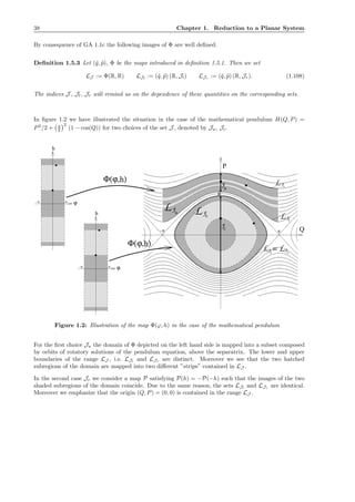
9. Introduction
The aim of this work is to study a particular type of miniature synchronous motor. Conventional syn-
chronous motors are characterized by the property that under working conditions the rotor exhibits a
stable rotation, the frequency being that of the power supply (hence the term ”synchronous”). In or-
der to enter the working conditions after switching on the motor, different techniques are suggested in
electrical engineering. Some of these techniques (such as pony motors, induction cages or electronic con-
trols) are rather complicated. Hence in many papers the transient behaviour upon start and the state
of synchronous rotation are treated separately. By contrast, the type of motor considered here features
a simple mechanism which permits a satisfactory physical modelling covering the entire process. This
model has been used by the manufacturer [12] for numerical studies and was presented in a colloquium
talk in the nineteen 80’s. It is represented by the following non–linear time–periodic system of ordinary
differential equations
d2
dτ2
ϑ = −
λ
J
i2
1 + i2
2 sin(ϕ) − ˜̺
d
dτ
ϑ − ˜m
U0 sin(ωτ) = R i1 + L
d
dτ
i1 + λ
d
dτ
sin(ϑ)
U0 sin(ωτ) = R i2 + L
d
dτ
i2 + λ
d
dτ
cos(ϑ) + u
d
dτ
u = i2/C.
(1)
The quantity ϑ is the angle of the rotor with respect to a fixed axis, i1 i2 correspond to the currents in
two parallel circuits and u describes the voltage of a condenser attached to the second power circuit.
Our approach for a mathematical treatise is based on perturbation theory. After some preliminary
transformations and assumptions on the parameters, the system turns out to be a special case of the
following problem
( ˙q, ˙p) = J∇H(q, p) + F(q, p, η, t, ε)
˙η = A η + G(q, p, t, ε).
(1.1)
This generalized problem consists of a one–degree of freedom Hamiltonian system (corresponding to the
mathematical pendulum in the above set of equations) and a linear system, the two being coupled by
small periodic perturbations. As this system is of interest by itself, we introduce a general framework
which might be of use elsewhere, too. The hypotheses we make reflect some of the features of the original
physical problem, however. As to the Hamiltonian system these assumptions include the existence of an
elliptic fixed point at the origin satisfying a non–resonance condition, as well as the existence of domains
foliated by periodic solutions (such as the oscillatory and rotatory solutions of the pendulum equation).
The matrix A is assumed to be exponentially asymptotically stable and the Fourier series with respect
to time t of the 2 π–periodic perturbations F and G are assumed to be finite.
v

10. vi Introduction
The original physical problem suggests two main questions. The discussion of the state of synchronous
rotation which is related to the existence and stability of a periodic solution near (q, p, η) = 0 and hence
is local in nature. On the other hand, solutions describing the transition from start to stationary rotation
are of upmost interest. They require a more global treatment. In a first part of this work a number of
key results for systems of type (1.1) are derived which prove to be a tool kit for concrete applications. In
a second part these results are applied to the miniature synchronous motor.
The first part is split into three self–contained chapters. In chapter 1 it is shown that the fixed point
(q, p, η) = 0 of the unperturbed system generates a unique 2 π–periodic solution. A discussion of its
stability is postponed until chapter 3. A time–dependant shift of the coordinates first yields a problem
which is again of type (1.1), i.e.
( ˙ˇQ, ˙ˇP) = J∇H( ˇQ, ˇP) + ˇF( ˇQ, ˇP, H, t, ε)
˙H = A H + ˇG( ˇQ, ˇP, t, ε),
(1.16)
but satisfies ˇF(0, 0, 0, t, ε) = 0 and ˇG(0, 0, t, ε) = 0. For ε = 0, the ( ˇQ, ˇP)–plane H = 0 corresponds to
the center manifold of the origin, whereas the H–axis ( ˇQ, ˇP) = (0, 0) represents the stable manifold. For
ε = 0 sufficiently small we establish the existence of an integral manifold ( ˇQ, ˇP) = V(t, H, ε), the so–called
strongly stable manifold. This is achieved by adapting a result of Kelley [8] to our situation. Applying
the transformation ( ˇQ, ˇP) = (Q, P) + V(t, H, ε) then yields a system of the form
( ˙Q, ˙P) = J∇H(Q, P) + ˆF(Q, P, H, t, ε)
˙H = A H + ˆG(Q, P, H, t, ε),
(1.87)
where in particular ˆF vanishes on the new H–axis, i.e.
ˆF(0, 0, H, t, ε) = 0 ˆG(0, 0, 0, t, ε) = 0. (1.88)
In a next step we replace (Q, P) by action–angle coordinates (ϕ, h) ∈ R2
. The transformed system is
equivalent to (1.87) if we restrict (Q, P) to regions of periodic solutions of ( ˙Q, ˙P) = J∇H(Q, P). In view
of (1.88) such a region may be a neighbourhood of the fixed point (Q, P, H) = (0, 0, 0) as well. In this
case, the set (h, H) = (0, 0) corresponds to (Q, P, H) = (0, 0, 0) and is invariant. The stability discussion
of (h, H) = (0, 0) therefore yields information on the stability of (Q, P, H) = (0, 0, 0) which eventually
corresponds to synchronous rotation in the case of our model of a synchronous motor. In action–angle
coordinates the system is of the form
˙ϕ = ω(h) + f(t, ϕ, h, H, ε)
˙h = g(t, ϕ, h, H, ε)
˙H = A H + h(t, ϕ, h, H, ε)
(1.110)
where A still denotes the matrix introduced in (1.1) and f, g, h vanish for ε = 0. The unperturbed
problem corresponding to (1.110) suggests the existence of an attractive invariant manifold near H = 0.
The majority of results on the existence of such manifolds (see e.g. Fenichel [4], Hirsch, Pugh, Shub
[6]) are based on a discussion of Lyapunov type numbers of solutions. For the purpose of this work
an approach based on more easily accessible quantities is more convenient, see Kirchgraber [9]. In this
work we apply an adaption by Nipp/Stoffer [13] where the assumptions are expressed in terms of the
vector field. It is here where the introduction of action–angle coordinates turns out to be advantageous.
The attractive invariant manifold we establish admits the representation H = S(t, ϕ, h, ε) with S = 0
for ε = 0. Since all solutions of (1.110) approach the invariant manifold, the discussion then reduces to
the reduced system, i.e. the restriction of eq. (1.110) to the attractive invariant manifold. This reduced
system is two–dimensional but non-autonomous. It is represented in two different forms, either of which
will be used in chapter 2 and chapter 3, respectively.

11. Introduction vii
The first representation of the reduced system given in chapter 1 is used for the global discussion. Taking
into account some additional properties of the original physical problem, chapter 2 deals with a system
of the form
˙ϕ = ω(h) +
3
j=2
εj
k,n∈Z
fj
k,n(h) ei(kϕ+nt)
+ ε4
f4
(t, ϕ, h, ε)
˙h =
3
j=2
εj
k,n∈Z
gj
k,n(h) ei(kϕ+nt)
+ ε4
g4
(t, ϕ, h, ε)
(2.1)
defined for ϕ, h ∈ R. Given km, nm ∈ Z and hm ∈ R such that gj
km,nm
= 0 (j ∈ {2, 3}) and km ω(hm) +
nm = 0 the value hm is called a resonance. We assume that the set of resonances hm is finite. Moreover,
for every resonance hm we require that d
dh ω(hm) = 0 holds. In order to obtain information on the
qualitative behaviour of (2.1) averaging techniques are applied. More precisely we apply time–dependant
near–identity transformations of the form ¯h = h + O(ε2
). This change of coordinates is defined in a
standard way, see Kirchgraber [11] or Sanders/Verhulst [17]. We use it in a somewhat different way,
however. As the transformation is singular in every resonance, it is applied outside a neighbourhood of
the resonances. In order to keep the higher order terms small, the size of the neighbourhood of each
resonance must be chosen appropriately. We show that the neighbourhoods omitted may be chosen to be
O(ε)–small. More precisely, for fixed δ > 0 and choosing |ε| < εO
(δ) the transformation may be applied
outside |ε|
δ –neighbourhoods of the resonances. In this outer region the transformed system then takes the
form
˙ϕ = ω(¯h) + O(ε)
˙¯h = ε2
g2
0,0(¯h) + ε2
δ2
¯g2
(t, ϕ, ¯h, ε, δ) + O(ε3
).
(2.23)
where ¯g2
is still bounded. If on a subset of the outer region the map g2
0,0 is bounded from below, the
parameters δ and |ε| < εO
(δ) may be chosen such that ˙¯h > 0 and thus all solutions leave this subset.
Away from zeroes of g2
0,0 the qualitative behaviour is therefore determined simply by the sign of g2
0,0.
In the inner region, i.e. if h satisfies |h − hm| < 4 |ε|
δ , a different near–identity change of coordinates is
defined. The resulting system then reads as follows
˙ϕ = ω(¯h) + O(ε2
)
˙¯h = ε2
g2
0,0(¯h) + ε2
l∈N∗
g2
lkm,lnm
(¯h) eil(kmϕ+nmt)
+ O(ε3
). (2.25)
Introducing the inner variables
ε ˜h := const ¯h − hm ∀ ¯h − hm < 4
|ε|
δ
ψ := km ϕ + nm t,
(2.28)
and taking into account again some special features which arise in the application of the synchronous
motor, the system takes the form of a km 2 π–periodically perturbed pendulum with external torque,
i.e. it is given by
˙ψ = ε ˜h + ε2 ˜f2
(t, ψ, ˜h, ε)
˙˜h = ε (a0 + ac
1 cos(ψ) + as
1 sin(ψ)) + ε2
˜g2
(t, ψ, ˜h, ε).
(2.29)
The quantities a0, ac
1 and as
1 are determined by the Fourier coefficients g2
0,0 and g2
km,nm
evaluated at
h = hm.

12. viii Introduction
We then treat the following two situations:
1. |a0| > (ac
1)
2
+ (as
1)
2
: For all solutions of the unperturbed system (i.e. (2.29) with the O(ε2
)–
terms dropped) the quantity
˙˜h is bounded from below. For ε sufficiently small, we conclude that
all solutions of (2.29) leave the region ¯h − hm < 4 |ε|
δ . This behaviour is refered to as passage
through resonance.
2. |a0| < (ac
1)2
+ (as
1)2
: The unperturbed system admits a hyperbolic and an elliptic fixed point on
the axis ˜h = 0, generating periodic solutions for (2.29). It then is possible that solutions starting
near the boundary ¯h − hm = 4 |ε|
δ are caught near ˜h = 0 as t → ∞. This effect is called capture
into resonance. Here it is shown, however, that the set of such solutions has size O(ε).
By consequence, the global qualitative behaviour of most solutions is known, once the values of g2
0,0 and
g2
km,nm
at h = hm are known. In chapter 4 the computation of these quantities will be the main point of
interest.
In chapter 3 we consider a system of the form
˙ϕ = Ω0 + f,0
(t, ϕ, ε) + P(h) f,1
(t, ϕ, ε) + P(h)
2
f,2
(t, ϕ, P(h), ε)
˙h = P(h)
d
dh P(h)
g,1
(t, ϕ, ε) + P(h)2
d
dh P(h)
g,2
(t, ϕ, ε) + P(h)3
d
dh P(h)
g,3
(t, ϕ, P(h), ε),
(3.1)
according to the second representation of the reduced system introduced in chapter 1. The use of an
analytical cutting function P in (3.1) is reminiscent of the way in which action–angle coordinates were
introduced. One may set P(h) = h in a neighbourhood of h = 0. We assume Ω0 ∈ 1
2 Z and that f,0
(t, ϕ, ε),
g,1
(t, ϕ, ε) admit the following Fourier representation with respect to ϕ
f,0
(t, ϕ, ε) = f,0
0 (t, ε) + f,0
c (t, ε) cos(2 ϕ) + f,0
s (t, ε) sin(2 ϕ)
g,1
(t, ϕ, ε) = g,1
0 (t, ε) − f,0
s (t, ε) cos(2 ϕ) + f,0
c (t, ε) sin(2 ϕ).
(3.2)
The maps f,1
, g,2
are assumed to be π–antiperiodic (i.e. f,1
(t, ϕ + π, ε) = −f,1
(t, ϕ, ε)). With the help
of Floquet’s theory we derive a near–identity transformation of the form
ϕ = ψ + u(t, ψ, ε) P(h) = r
v(t, ε)
1 + ∂ψu(t, ψ, ε)
(3.4)
transforming (3.1) to the form
˙ψ = ˜Ω(ε) + O(r)
˙r = r g,1
0,0(ε) + r2
ˆg,2
(t, ψ, ε) + r3
ˆg,3
(t, ψ, r, ε)
(3.20)
where ˜Ω(0) = Ω0. Hence the coefficient g,1
0,0(ε) provides a criterion for {r = 0} (and thus {h = 0})
to be asymptotically stable, or unstable, respectively. The quantity g,1
0,0(ε) will be evaluated in chapter
4, in order to prove asymptotic stability of the periodic solution near (q, p, η) = (0, 0, 0) in case of the
synchronous motor problem.

13. Introduction ix
In the second part, chapter 4, we present the application of part one to the model of a miniature
synchronous motor mentioned before. After some preliminary preparations eq. (1) is transformed into
˙q = p
˙p = −
a
2
2
sin(q) + ε (η1 cos(q + t) − η2 sin(q + t)) − ε2
̺ p − ε2
(m + ̺)
˙η1 = −η1 + ε sin(q + t)
˙η2 = −η2 − 2 η3 + ε cos(q + t)
˙η3 = η2 − ε cos(q + t).
(4.14)
The quantity a is rougly equal to λ
R . For fixed a the perturbation parameter ε is given by a λ
U0
.
Here we assume that the voltage U0 of the power supply and the moment of inertia J of the motor are
proportional. Thus, ε tends to 0 provided U0 (and thus J) increases, while the magnetic dipol λ, and the
resistance R are kept fixed. By consequence, the effect of induction generated by the rotating permanent
magnet and exerted on the coils decreases as ε → 0.
In order to obtain preliminary insight into the features of (4.14) we present the results of various nu-
merical simulations carried out with the help of the package dstool [3]. The results found confirm the
analytical discussion given later in this chapter. In addition, they demonstrate that the behaviour in a
neighbourhood of the separatrix of the unperturbed problem of (4.14) is of no particular interest if a is
large. (Since the techniques introduced in part one rely on regions of periodic solutions of the Hamiltonian
system, the neighbourhood of a separatrix is not covered by our analytical approach.)
The main task in chapter 4 is to apply the tools of part one to system (4.14) and to compute the key
quantities g2
0,0(h), g2
km,nm
(h) and g,1
0,0(ε). Among other things this amounts to explicitely construct
suitable approximations of the invariant manifolds introduced in chapter 1. The introduction of action–
angle coordinates associated with the pendulum equation, is based on Fourier series of Jacobian elliptic
functions. Eventually g2
0,0(h) and g2
km,nm
(h) are represented with the help of convolutions of Fourier
series. The complexity of this procedure requires the use of a software package for symbolic and numerical
computations. The author has chosen the Maple [15] software package. Its synthax is simple and legible
for readers with basic knowledge in programming. Hence the source code listed is comprehensible to a
growing community. For various choices of the parameters the dynamics of the model is discussed in terms
of the physical behaviour of the motor. The influence of a mechanical friction (given by the parameter
˜̺) and an external torque ( ˜m) is considered as well. Both situations considered in chapter 2, i.e. the
case of passage of all solutions up to an O(ε)–set as well as the passage of strictly all solutions through
resonances are established. The periodic solution near the origin, corresponding to the synchronous
rotation of the shaft, is shown to be stable for all choices of the parameters. Moreover additional results
are established: the possibility of asynchronous rotations, the modulation of the synchronous rotation
state by a second harmonic as well as a synchronous rotation with large variation of the angular speed
(caused by a capture into resonance). The overall conclusion is that for sufficiently large a the motor
behaves favouritely, i.e. enters the state of stable synchronous rotation when switched on.
Chapter 4 closes with a result on the separatrix region for sufficiently small values of the parameter
a. In this situation, the existence of a global attractive invariant manifold of (4.14) is established. The
corresponding reduced system then is of periodically perturbed pendulum type. Although an approximate
representation of the reduced system is not available, the construction of an approximate Melnikov
function is feasible. The numerical evaluation of the corresponding formula then confirms the results
found by numerical simulation. More precisely, it is established that solutions starting with a frequency
larger than the frequency of the power supply may either enter the state of synchronous rotation or the
frequency may eventually tend to zero.

15. Chapter 1
Reduction to a Planar System
1.1 The System under Consideration
1.1.1 The Differential Equations
In this chapter we consider autonomous ordinary differential equations with a nonautonomous time–
periodic perturbation. For the unperturbed case we assume two independent subsystems, a Hamiltonian
system of one degree of freedom and a stable linear system. More precisely we will discuss equations of
the form
( ˙q, ˙p) = J∇H(q, p) + F(q, p, η, t, ε)
˙η = A η + G(q, p, t, ε),
(1.1)
where (q, p) ∈ R2
, η ∈ Rd
and J := 0
−1
1
0 represents the symplectic normal form.
We assume that A ∈ Rd×d
has only eigenvalues on the left complex halfplane. The Hamiltonian H is
assumed to be of class Cω
(i.e. analytical), the maps F, G are assumed to be Cω
, 2π–periodic with
respect to the time–variable t and vanishing as ε → 0.
1

16. 2 Chapter 1. Reduction to a Planar System
1.1.2 General Assumptions on the System
In this chapter we assume the following statements to be true
GA 1.1. The unperturbed Hamiltonian system
( ˙q, ˙p) = J∇H(q, p) (1.2)
satisfies the following set of assumptions :
(a) System (1.2) admits an elliptic fixed point in the origin. More precisely we assume that
in this situation ∇H(0, 0) = 0, ∂q∂pH(0, 0) = 0 and ∂2
q H(0, 0), ∂2
pH(0, 0) > 0. Moreover
D3
H(0, 0) = 0 holds and Ω0 := ∂2
q H(0, 0) ∂2
pH(0, 0) ∈ N := {0, 1, 2, . . .}.
(b) There exist an interval J = (Jl, Jr) together with a mapping Ω ∈ Cω
(J , R) such that the
solution (q, p)(t; 0, p0) of (1.2) with initial value (0, p0), p0 ∈ J at time t = 0 is periodic in t
with frequency Ω(p0) > 0.
(c) There is an integer r ≥ 0 such that for every 0 ≤ k ≤ r+7 the limit of ∂k
p0
Ω(p0) for p0 → Jl, Jr
exists and does not vanish for k = 0. If 0 ∈ J then lim
p0→0
∂p0 Ω(p0) = 0.
GA 1.2. The real parts of the eigenvalues of A are all negative, bounded by a suitable constant c0 > 0:
ℜ(σ(A)) ≤ −c0.
Here and in what follows, σ(A) denotes the spectrum, i.e. the set of all eigenvalues of the matrix
A. Moreover we assume that A is diagonalizable.
GA 1.3. Consider the Taylor expansion of order 3 in ε = 0 of the maps F and G, i.e. the representation
F(q, p, η, t, ε) =
3
j=1
εj
Fj
(q, p, η, t) + ε4
F4
(q, p, η, t, ε)
G(q, p, t, ε) =
3
j=1
εj
Gj
(q, p, t) + ε4
G4
(q, p, t, ε).
(1.3)
We assume that the maps Fj
, Gj
, j = 1, 2, 3 in (1.3) admit a representation as finite Fourier series1
of degree N ∈ N with respect to t , i.e.
Fj
(q, p, η, t) =
|n|≤N
Fj
n(q, p, η) eint
Gj
(q, p, t) =
|n|≤N
Gj
n(q, p) eint
. (1.4)
GA 1.4. The map F is affine with respect to η, i.e. ∂k
η F(q, p, η, t, ε) = 0 for all k ≥ 2.
1Note that the functions F j
n, Gj
n, n ∈ {−N, . . . , N}, j = 1, 2, 3 are complex valued functions. As system (1.1) is real, it
is easy to see that F j
n = ¯F j
−n, Gj
n = ¯Gj
−n, i.e. the complex conjugate valued functions.

17. 1.1. The System under Consideration 3
1.1.3 A Short Overview on the Strategy Followed
The aim of this first chapter is to derive a plane (non–autonomous) system which asymptotically de-
termines the qualitative behaviour of system (1.1). Considering (1.1) in the unperturbed case (ε = 0)
we see that due to the stability of the matrix A (as assumed in GA 1.2), all solutions tend towards the
(q, p)–plane η = 0. Hence the asymptotic behaviour in the unperturbed case is determined by the plane
Hamiltonian system (1.2).
In the case of a small perturbation (ε = 0 but small) we aim on a reduction to a plane system as
well. However, it will be necessary to consider different regions of the (q, p) phase space separately in
order to derive appropriate coordinates. Using invariant manifold theory we then show the existence
of an attractive two-dimensional (time–dependent) invariant manifold for the corresponding region and
consider the system restricted to this manifold. Following this way we yield a plane system, representing
the asymptotic behaviour in the corresponding domain for the perturbed case as well.
In sections 1.2–1.4 we deal with regions of periodic solutions of the Hamiltonian system (1.2) near an
elliptic fixed point. (Note that the fixed point itself is not included in such a region). As the plane
Hamiltonian system admits an elliptic fixed point at (q, p) = (0, 0), there exists a periodic solution of
the perturbed 2 + d–dimensional system (1.1) near the origin. This is dealed with in section 1.2. Since
the stability of this periodic solution is essential for the asymptotic behaviour of (1.1), we will perform
changes of coordinates in a way such that the region considered may be extended into this periodic
solution. This will be prepared in section 1.4.
Sections 1.5–1.6 deal with any region of periodic solutions of the Hamiltonian system. Introducing action
angle coordinates in section 1.5 it will be possible to establish the existence of an attractive invariant
manifold in section 1.6 and consider the ”restricted” plane system on the region chosen.
The entire process carried out in chapter 1 and chapter 2 will be presented in a form sufficiently explicit
for application on concrete examples. This requires more work in the theoretical part but on the other
hand leads to a form applicable in many situations. Moreover the author has tried to present the steps
carried out in a ”modular” manner, such that the results of certain sections may be applied independently.

18. 4 Chapter 1. Reduction to a Planar System
1.2 The Periodic Solution
1.2.1 The Existence of a Unique Periodic Solution Near the Origin
As mentioned above, in this section we consider the case where the Hamiltonian system (1.2) admits an
elliptic fixed point at the origin. The aim is to establish the existence of a unique 2π–periodic solution
of system (1.1) (for ε sufficiently small), located near the elliptic fixed point at the origin. This will be
carried out by applying the following general result to our situation.
Lemma 1.2.1 Consider an ordinary differential equation of the form
˙x = εp
(f(x) + g(x, t, ε)) , x ∈ Rm
(1.5)
where p ∈ N and f(0) = 0. Let f and g be of class C ˜r
(˜r ≥ 1 or ˜r = ω) and assume that g is T –
periodic with respect to t and vanishes for ε = 0, i.e. g(x, t, 0) = 0 ∀x ∈ Rm
, ∀t ∈ R. Moreover, let
σ (Df(0)) ∩ i 2π
T Z = ∅ if p = 0 and det Df(0) = 0 if p > 0.
Then there exists an ε1 > 0 and a unique map ˇx ∈ C ˜r
(R × (−ε1, ε1), Rm
) such that ˇx(t, 0) = 0 (∀t ∈ R)
and for every |ε| < ε1, the mapping t → ˇx(t, ε) is a T –periodic solution of system (1.5).
PROOF: We prove this lemma in several steps.
1. First, define the map
˜g(x, t, ε) := f(x) − Df(0) x + g(x, t, ε)
for x ∈ Rm
, t ∈ R and ε ∈ R. Then we see that ˜g is T –periodic with respect to t,
˜g(0, t, 0) = 0 and ∂x˜g(0, t, 0) = ∂xg(0, t, 0) = 0. (1.6)
Using this map ˜g we may write (1.5) as follows:
˙x = εp
(Df(0) x + ˜g(x, t, ε)) . (1.7)
Let x(t; t0, x0, ε) denote the solution of (1.5) with initial value x0 at time t0. By the uniqueness of
solutions we have
x(t; t0, x0, ε) = x(t; t1, x(t1; t0, x0, ε), ε). (1.8)
Since ˜g(x, t, ε) is T –periodic with respect to t, it follows that the flow induced by (1.5) is T –periodic
as well, hence
x(t; t0, x0, ε) = x(t + T ; t0 + T, x0, ε). (1.9)
As g vanishes for ε = 0 we finally note that x = 0 is a solution of (1.5) for ε = 0, hence
x(t; t0, 0, 0) = 0 ∀t, t0 ∈ R. (1.10)

19. 1.2. The Periodic Solution 5
2. In a next step we shall establish the existence of a unique initial value ξ(ε) near x = 0 which
corresponds to a T –periodic solution of (1.5). This will be shown by applying the Implicit Function
Theorem to the following map:
R(ε, ξ) :=
1
εp T
eεp
T Df(0)
− IR 2+d ξ +
1
T
T
0
eεp
(T −s) Df(0)
˜g(x(s; 0, ξ, ε), s, ε) ds.
Under the conditions assumed, R ∈ C ˜r
(R × Rm
, Rm
). By (1.6) and (1.10) we find
R(0, ξ) =
1
T eT Df(0)
− IR 2+d ξ p = 0
Df(0) ξ p > 0
such that R(0, 0) = 0. Taking the partial derivative of R(0, ξ) we find
∂ξR(0, 0) =
1
T eT Df(0)
− IR 2+d p = 0
Df(0) p > 0.
Since by assumption σ (Df(0)) ∩ i 2π
T Z = ∅ (if p = 0) and det Df(0) = 0 (if p > 0), we see that
det(∂ξR(0, 0)) =



1
T det eT Df(0)
− IR 2+d = 1
T
λ∈σ(Df(0))
(eT λ
− 1) = 0 p = 0
det Df(0) = 0 p > 0.
Hence it follows by the Implicit Function Theorem that there exists an ε1 > 0 as well as a unique
map ξ ∈ C ˜r
((−ε1, ε1), Rm
) with ξ(0) = 0 such that for every |ε| < ε1, R(ε, ξ(ε)) = 0.
In accordance with the representation (1.7) we write the solution x(t; 0, ξ0, ε) of (1.5) with initial
value ξ0 at time t0 = 0 using the Variation of Constant formula, i.e.
x(t; 0, ξ0, ε) = eεp
t Df(0)
ξ0 + εp
t
0
eεp
(t−s) Df(0)
˜g(x(s; 0, ξ0, ε), s, ε) ds.
By definition of R we thus find
R(ε, ξ) = 0 ⇔ εp
T R(ε, ξ) = 0 ⇔ ξ = x(T ; 0, ξ, ε). (1.11)
Setting ξ = ξ(ε) therefore yields ξ(ε) = x(T ; 0, ξ(ε), ε).
3. It remains to show that for fixed |ε| < ε1 the initial value ξ(ε) generates a periodic solution of (1.5),
indeed. We therefore define ˇx(t, ε) := x(t; 0, ξ(ε), ε). Applying (1.8), (1.9) and (1.11) we find for
any t ∈ R
ˆx(t + T, ε) = x(t + T ; 0, ξ(ε), ε) = x(t + T ; T, x(T ; 0, ξ(ε), ε), ε)
= x(t; 0, x(T ; 0, ξ(ε), ε), ε) = x(t; 0, ξ(ε), ε)
= ˇx(t, ε).
Hence the solution ˇx(t, ε) with initial value ˇx(0, ε) = ξ(ε) is T –periodic .
Moreover, ξ(0) = 0 together with (1.10) imply
ˇx(t, 0) = x(t; 0, ξ(0), 0) = x(t; 0, 0, 0) = 0.

20. 6 Chapter 1. Reduction to a Planar System
4. With the help of the statements given by the Implicit Function Theorem on the uniqueness, range
and domain of the map ξ, it eventually may be shown that the map t → ˇx(t, ε) is the only T –periodic
solution close to the origin satisfying ˇx(t, 0) = 0.
Therefore the statement given in lemma 1.2.1 is proved.
It now is a simple consequence of the preceeding lemma that system (1.1) admits a unique 2π–periodic
solution (ˇq, ˇp, ˇη) close to the origin. This is carried out in the following lemma.
Lemma 1.2.2 There exists ε1 > 0 as well as a unique map (ˇq, ˇp, ˇη) ∈ Cω
(R × (−ε1, ε1), R2+d
) such
that for fixed |ε| < ε1 the map t → (ˇq, ˇp, ˇη)(t, ε) is a 2π–periodic solution of (1.1) and for ε = 0,
(ˇq, ˇp, ˇη)(t, 0) = 0 ∀t ∈ R.
For simplicity we will omit the parameter a in the notation (ˇq, ˇp, ˇη) unless needed explicitely.
PROOF: For x = (q, p, η) ∈ R2+d
we set
f(x) := f(q, p, η) :=
J∇H(q, p)
A η
g(x, t, ε) := g(q, p, η, t, ε) :=
F(q, p, η, t, ε)
G(q, p, t, ε)
.
By assumption GA 1.1a we have f(0) =
J∇H(0, 0)
A 0
= 0 and
σ(Df(0)) = σ
JD2
H(0, 0) 0
0 A
= σ(JD2
H(0, 0)) ∪ σ(A), (1.12)
such that from σ JD2
H(0, 0) = ± i ∂2
q H(0, 0) ∂2
pH(0, 0) and GA 1.1a together with GA 1.2 we
deduce σ (Df(0)) ∩ i Z = ∅.
Taking into account the assumptions made in section 1.1.1 for F, G and H it is readily seen that we are
in the position to apply lemma 1.2.1 (where m = 2 + d, p = 0, ˜r = ω and T = 2π). Hence the proof of
lemma 1.2.2 is a consequence of lemma 1.2.1.

21. 1.2. The Periodic Solution 7
1.2.2 The Transformation into the Periodic Solution
The purpose of this section is to transform the coordinates of system (1.1) in a way, such that the origin
becomes a fixed point. This may be done by performing a (time–dependent) translation into the periodic
solution (ˇq, ˇp, ˇη).
More precisely we will use the Taylor / Fourier expansions (1.3), (1.4) assumed in GA 1.3 to explicitely
calculate a similar representation of the corresponding vector field in the new coordinates. This will be
prepared in the following lemma:
Lemma 1.2.3 Consider a linear inhomogenous differential equation on R2+d
of the following type
˙x = B x +
|n|≤N
bneint
, (1.13)
where bn ∈ C2+d
for every |n| ≤ N, bn = b−n and σ (B)∩i Z = ∅. Then there exists a unique 2π–periodic
solution given by
x(t) =
|n|≤N
[i n IC 2+d − B]−1
bn eint
. (1.14)
PROOF: Note first that since σ (B) ∩i Z = ∅, the inverse of the matrix i n IC 2+d − B exists. It is evident
that the function x presented in (1.14) is 2π–periodic with respect to t. Moreover
˙x(t) − B x(t) =
|n|≤N
i n [i n IC 2+d − B]
−1
bn eint
− B
|n|≤N
[i n IC 2+d − B]
−1
bn eint
=
|n|≤N
[i n IC 2+d − B] [i n IC 2+d − B]
−1
bn eint
=
|n|≤N
bn eint
,
such that x is a solution of (1.13), indeed.
Consider any further 2π–periodic solution y of (1.13). Writing its Fourier expansion y =
n∈N
cn eint
and
calculating ˙y−B y one then compares the result with
|n|≤N
bn eint
which implies cn = [i n IC 2+d − B]
−1
bn
and thus x = y. Hence x is unique as claimed.
We now are in the position to prove the main result of this section.
Proposition 1.2.4 Let (ˇq, ˇp, ˇη) denote the 2π–periodic solution of system (1.1) for |ε| < ε1, asserted in
lemma 1.2.2 and perform the following change of coordinates in the (q, p, η, t, ε)–space:
(q, p, η, t, ε) = ((ˇq, ˇp, ˇη)(t, ε), 0, 0) + ( ˇQ, ˇP, H, t, ε), (1.15)

22. 8 Chapter 1. Reduction to a Planar System
where2
( ˇQ, ˇP) ∈ R2
, H ∈ Rd
, t ∈ R and |ε| < ε1. Then (1.1) transforms into the system
( ˙ˇQ, ˙ˇP) = J∇H( ˇQ, ˇP) + ˇF( ˇQ, ˇP, H, t, ε)
˙H = A H + ˇG( ˇQ, ˇP, t, ε),
(1.16)
where the following statements hold :
• The mappings ˇF and ˇG are of class Cω
, vanish at the origin ( ˇQ, ˇP, H) = 0 and admit the repre-
sentation3
ˇF( ˇQ, ˇP, H, t, ε) =
3
j=1
εj ˇFj
( ˇQ, ˇP, H, t) + ε4 ˇF4
( ˇQ, ˇP, H, t, ε)
ˇG( ˇQ, ˇP, t, ε) =
3
j=1
εj ˇGj
( ˇQ, ˇP, t) + ε4 ˇG4
( ˇQ, ˇP, t, ε)
(1.17)
where ˇFj
and ˇGj
, (j = 1, . . . , 4) are 2π–periodic with respect to t.
• The map H → ˇF( ˇQ, ˇP, H, t, ε) is affine.
• The mappings ˇF1
, ˇF2
, ˇG1
and ˇG2
may be expressed in terms of the original vector field of system
(1.1):
ˇF1
( ˇQ, ˇP, H, t) = F1
( ˇQ, ˇP, H, t) −
|n|≤N
∆(n, ˇQ, ˇP) F1
n(0, 0, 0) eint
ˇF2
( ˇQ, ˇP, H, t) = F2
( ˇQ, ˇP, H, t) −
|n|≤N
∆(n, ˇQ, ˇP) F2
n(0, 0, 0)eint
+
|n|,|¯n|≤N
1
2 JD3
H( ˇQ, ˇP) α1,1
n,1, α1,1
¯n,1
+ ∂(q,p)F1
n( ˇQ, ˇP, H) − ∆(n + ¯n, ˇQ, ˇP) ∂(q,p)F1
n (0, 0, 0) α1,1
¯n,1
+ ∂ηF1
n( ˇQ, ˇP, H) − ∆(n + ¯n, ˇQ, ˇP) ∂ηF1
n(0, 0, 0) α1,1
¯n,2 ei(n+˜n)t
ˇG1
( ˇQ, ˇP, t) = G1
( ˇQ, ˇP, t) − G1
(0, 0, t)
ˇG2
( ˇQ, ˇP, t) = G2
( ˇQ, ˇP, t) − G2
(0, 0, t) +
|n|,|¯n|≤N
∂(q,p)G1
n( ˇQ, ˇP) − ∂(q,p)G1
n(0, 0) α1,1
¯n,1
(1.18)
where
∆(n, ˇQ, ˇP) := [i n IC 2 − JD2
H( ˇQ, ˇP)] i n IC 2 − JD2
H(0, 0)
−1
α1,1
n,1 = i n IC 2 − JD2
H(0, 0)
−1
F1
n(0, 0, 0)
α1,1
n,2 = [i n IC d − A]
−1
G1
n(0, 0).
(1.19)
2The letter H must be read as ”upper eta”
3for the application in chapter 4 it suffices to consider the expansions including terms of order O(ε2) of ˇF and of order
O(ε) of ˇG. The formulae for O(ε3)–terms are provided in order to enable a more detailed discussion on the capture in
resonance, cf. section 2.3.5.

23. 1.2. The Periodic Solution 9
• Moreover, ˇF1
, ˇF2
, ˇG1
and ˇG2
may be represented as Fourier polynomials in t, similar to the
representation (1.4), i.e.
ˇFj
( ˇQ, ˇP, H, t) =
|n|≤jN
ˇFj
n( ˇQ, ˇP, H, t) eint ˇGj
( ˇQ, ˇP, t) =
|n|≤jN
ˇGj
n( ˇQ, ˇP, t) eint
(1.20)
• The values of the map ˇF3
may be expressed in an analogous way:
ˇF3
( ˇQ, ˇP, H, t) =F3
( ˇQ, ˇP, H, t) −
|n|≤N
∆(n, ˇQ, ˇP) F3
n(0, 0, 0)eint
+
|n|,|¯n|≤N
JD3
H( ˇQ, ˇP) α1,1
n,1, α2,1
¯n,1
+ ∂(q,p)F2
n( ˇQ, ˇP, H) − ∆(n + ¯n, ˇQ, ˇP) ∂(q,p)F2
n(0, 0, 0) α1,1
¯n,1
+ ∂ηF2
n( ˇQ, ˇP, H) − ∆(n + ¯n, ˇQ, ˇP) ∂ηF2
n(0, 0, 0) α1,1
¯n,1
+ ∂(q,p)F1
n( ˇQ, ˇP, H) − ∆(n + ¯n, ˇQ, ˇP) ∂(q,p)F1
n(0, 0, 0) α2,1
¯n,1
+ ∂ηF1
n( ˇQ, ˇP, H) − ∆(n + ¯n, ˇQ, ˇP) ∂ηF1
n(0, 0, 0) α2,1
¯n,1 ei(n+¯n)t
+
|n|,|¯n|,|˜n|≤N
JD3
H( ˇQ, ˇP) α1,1
n,1, α2,2
¯n,˜n,1
+ 1
6 JD4
H( ˇQ, ˇP) − ∆(n + ¯n + ˜n, ˇQ, ˇP) JD4
H(0) α1,1
n,1 α1,1
¯n,1 α1,1
˜n,1
+ 1
2 ∂2
(q,p)F1
n( ˇQ, ˇP, H) − ∆(n + ¯n + ˜n, ˇQ, ˇP) ∂2
(q,p)F1
n(0, 0, 0) α1,1
¯n,1, α1,1
˜n,1
+ 1
2 ∂η∂(q,p)F1
n( ˇQ, ˇP, H) − ∆(n + ¯n + ˜n, ˇQ, ˇP) ∂η∂(q,p)F1
n(0, 0, 0) α1,1
˜n,1, α1,1
¯n,2
+ 1
2 ∂(q,p)∂ηF1
n( ˇQ, ˇP, H) − ∆(n + ¯n + ˜n, ˇQ, ˇP) ∂(q,p)∂ηF1
n(0, 0, 0) α1,1
˜n,2, α1,1
¯n,1
+ ∂(q,p)F1
n( ˇQ, ˇP, H) − ∆(n + ¯n, ˇQ, ˇP) ∂(q,p)F1
n (0, 0, 0) α2,2
¯n,˜n,1
+ ∂ηF1
n( ˇQ, ˇP, H) − ∆(n + ¯n, ˇQ, ˇP) ∂ηF1
n(0, 0, 0) α2,2
¯n,˜n,1 ei(n+¯n+˜n)t
.
(1.21)
where in addition
α2,1
n,1 = i n IC 2 − JD2
H(0, 0)
−1
F2
n(0, 0, 0) α2,1
n,2 = [i n IC d − A]
−1
G2
n(0, 0)
α2,2
n,¯n,1 = i (n + ¯n) IC 2 − JD2
H(0, 0)
−1
∂(q,p)F1
n(0, 0, 0) α1,1
n,1 + ∂ηF1
n(0, 0, 0) α1,1
n,2 .
PROOF: In order to simplify the notation, we use the same abbreviations as introduced in the proof of
lemma 1.2.2:
x := (q, p, η) ˇx(t, ε) :=(ˇq, ˇp, ˇη)(t, ε) y := ( ˇQ, ˇP, H)
f(x) :=
J∇H(q, p)
A η
g(x, t, ε) :=
F(q, p, η, t, ε)
G(q, p, t, ε)
(1.22)
such that system (1.1) defined for x ∈ R2+d
reads
˙x = f(x) + g(x, t, ε). (1.23)

24. 10 Chapter 1. Reduction to a Planar System
In view of assumption GA 1.3 we rewrite g(x, t, ε) as follows:
g(x, t, ε) =
3
j=1
εj
gj
(x, t) + ε4
g4
(x, t, ε) =
3
j=1
εj
|n|≤N
gj
n(x) eint
+ ε4
g4
(x, t, ε) (1.24)
where we have set
gj
n(x) =
Fj
n(q, p, η)
Gj
n(q, p)
∈ Cω
(R2+d
, C2+d
), |n| ≤ N, j = 1, 2, 3
and
g4
(x, t, ε) =
F4
(q, p, η, t, ε)
G4
(q, p, t, ε)
∈ Cω
(R2+d
× R × R, R2+d
).
The transformation defined in (1.15) corresponds to the time–dependent, 2π–periodic translation
x = ˇx(t, ε) + y
defined for t ∈ R and |ε| < ε1. Expressing (1.23) in the new coordinates yields
˙y = f(ˇx(t, ε) + y) + g(ˇx(t, ε) + y, t, ε) − ˙ˇx(t, ε) =: ˜f(y, t, ε). (1.25)
Note that ˜f ∈ Cω
(R2+d
× R × (−ε1, ε1), R2+d
) as f, g and ˇx are of class Cω
. As ˇx(t, ε) is a solution of
(1.1) and hence of (1.23) as well, we find
˜f(0, t, ε) = 0. (1.26)
Moreover, as ˇx and g vanish for ε = 0, it follows at once that
˜f(y, t, 0) = f(y). (1.27)
Since the last d components of
˜f(y, t, ε) − ˜f(y, t, 0) =
J ∇H(ˇq + ˇQ, ˇp + ˇP)
A (ˇη + H)
+
F(ˇq + ˇQ, ˇp + ˇP, ˇη + H, t, ε)
G(ˇq + ˇQ, ˇp + ˇP, t, ε)
−
J ∇H( ˇQ, ˇP)
A H
− ˙ˇx(t, ε)
=
J ∇H(ˇq + ˇQ, ˇp + ˇP) − J ∇H( ˇQ, ˇP) − J∇H(ˇq, ˇp)
A ˇη
+
F(ˇq + ˇQ, ˇp + ˇP, ˇη + H, t, ε) − F(ˇq, ˇp, ˇη, t, ε)
G(ˇq + ˇQ, ˇp + ˇP, t, ε) − G(ˇq, ˇp, t, ε)
(1.28)
do not depend on H, we may split this vector ˜f(y, t, ε) − ˜f(y, t, 0) into a two–dimensional component
which depends on H and a second, d–dimensional component, independent of H. More precisely we are
in the position to introduce the following abbreviations :
ˇF( ˇQ, ˇP, H, t, ε)
ˇG( ˇQ, ˇP, t, ε)
:= ˜f(y, t, ε) − ˜f(y, t, 0)
We continue with the following steps:

25. 1.2. The Periodic Solution 11
1. Consider the Taylor expansion of ˜f at ε = 0, i.e. the representation
˜f(y, t, ε) = ˜f(y, t, 0) + ε ∂ε
˜f(y, t, 0) + 1
2 ε2
∂2
ε
˜f(y, t, 0) + 1
6 ε3
∂3
ε
˜f(y, t, 0) + ε4 ˜f4
(y, t, ε) (1.29)
where ˜f4
(y, t, ε) is of class Cω
(R2+d
× R × (−ε1, ε1), R2+d
) and 2π–periodic with respect to t.
Setting
ˇFj
( ˇQ, ˇP, H, t)
ˇGj
( ˇQ, ˇP, t)
:= 1
j! ∂j
ε
˜f(y, t, 0) j = 1, 2, 3
ˇF4
( ˇQ, ˇP, H, t, ε)
ˇG4
( ˇQ, ˇP, t, ε)
:= ˜f4
(y, t, ε),
(1.30)
and taking into account that (1.26), (1.28) imply
ˇF(0, 0, 0, t, ε)
ˇG(0, 0, t, ε)
= −f(0) = 0
we find the first statement claimed to be proved at once.
2. In order to prove the second statement we note that by (1.28), (1.30)
ˇF( ˇQ, ˇP, H, t, ε) = J ∇H(ˇq + ˇQ, ˇp + ˇP) − J ∇H( ˇQ, ˇP) − J∇H(ˇq, ˇp)
+ F(ˇq + ˇQ, ˇp + ˇP, ˇη + H, t, ε) − F(ˇq, ˇp, ˇη, t, ε)
such that the affinity of F assumed in GA 1.4 implies the affinity of ˇF ( with respect to H).
3. We determine the Taylor coefficients in (1.29).
Using (1.26) we have
∂j
ε
˜f(0, t, 0) = 0 j = 1, 2, 3. (1.31)
On the other hand, from definition (1.25) we derive
∂ε
˜f(y, t, ε) = Df(ˇx(t, ε) + y) ∂ε ˇx(t, ε) + ∂xg(ˇx(t, ε) + y, t, ε) ∂εˇx(t, ε)
+ ∂εg(ˇx(t, ε) + y, t, ε) − ∂ε ˙ˇx(t, ε),
(1.32)
∂2
ε
˜f(y, t, ε) = D2
f(ˇx(t, ε) + y) ∂εˇx(t, ε)[2]
+ Df(ˇx(t, ε) + y) ∂2
ε ˇx(t, ε)
+ ∂2
xg(ˇx(t, ε) + y, t, ε) ∂εˇx(t, ε)[2]
+ ∂xg(ˇx(t, ε) + y, t, ε) ∂2
ε ˇx(t, ε)
+ 2 ∂ε∂xg(ˇx(t, ε) + y, t, ε) ∂εˇx(t, ε) + ∂2
ε g(ˇx(t, ε) + y, t, ε)
− ∂2
ε
˙ˇx(t, ε)
(1.33)
∂3
ε
˜f(y, t, ε) = D3
f(ˇx(t, ε) + y) ∂ε ˇx(t, ε)[3]
+ 3 D2
f(ˇx(t, ε) + y) (∂ε ˇx(t, ε), ∂2
ε ˇx(t, ε)) + Df(ˇx(t, ε) + y) ∂3
ε ˇx(t, ε)
+ ∂3
xg(ˇx(t, ε) + y, t, ε) ∂εˇx(t, ε)[3]
+ 3 ∂2
xg(ˇx(t, ε) + y, t, ε) (∂εˇx(t, ε), ∂2
ε ˇx(t, ε)) + ∂xg(ˇx(t, ε) + y, t, ε) ∂3
ε ˇx(t, ε)
+ 3 ∂ε∂2
xg(ˇx(t, ε) + y, t, ε) ∂εˇx(t, ε)[2]
+ 3 ∂2
ε ∂xg(ˇx(t, ε) + y, t, ε) ∂ε ˇx(t, ε)
+ 3 ∂ε∂xg(ˇx(t, ε) + y, t, ε) ∂2
ε ˇx(t, ε) + ∂3
ε g(ˇx(t, ε) + y, t, ε)
− ∂3
ε
˙ˇx(t, ε)
(1.34)

26. 12 Chapter 1. Reduction to a Planar System
where the notation v[j]
must be understood as applying the corresponding multilinear–form on the
j vectors (v, . . . , v). Taking into account that by (1.24)
∂j
xg(y, t, 0) = 0 j = 1, 2, 3 ∂ε∂j
xg(y, t, 0) = ∂j
xg1
(y, t) j = 0, 1, 2
∂2
ε ∂j
xg(y, t, 0) = 2 ∂j
xg2
(y, t) j = 0, 1 ∂3
ε g(y, t, 0) = 6 g3
(y, t),
we therefore see that setting ε = 0, (1.32), (1.33) and (1.34) reduce to
∂ε
˜f(y, t, 0) = Df(y) ∂ε ˇx(t, 0) + g1
(y, t) − ∂t∂ε ˇx(t, 0)
∂2
ε
˜f(y, t, 0) = D2
f(y) ∂ε ˇx(t, 0)[2]
+ Df(y) ∂2
ε ˇx(t, 0)
+ 2 ∂xg1
(y, t) ∂ε ˇx(t, 0) + 2 g2
(y, t) − ∂t∂2
ε ˇx(t, 0)
∂3
ε
˜f(y, t, 0) = D3
f(y) ∂ε ˇx(t, 0)[3]
+ 6 D2
f(y) (∂ε ˇx(t, 0), 1
2 ∂2
ε ˇx(t, 0)) + Df(y) ∂3
ε ˇx(t, 0)
+ 3 ∂2
xg1
(y, t) ∂ε ˇx(t, 0)[2]
+ 6 ∂xg2
(y, t) ∂ε ˇx(t, 0)
+ 6 ∂xg1
(y, t) 1
2 ∂2
ε ˇx(t, 0) + 6 g3
(y, t)
− ∂t∂3
ε ˇx(t, 0).
(1.35)
4. In a next step we compute the functions ∂ε ˇx(t, 0), ∂2
ε ˇx(t, 0) and ∂3
ε ˇx(t, 0) by solving differential
equations :
Recall that by GA 1.1a D3
H(0, 0) = 0 such that by definition of f, D2
f(0) = 0. Therefore (1.24)
together with (1.31), (1.35) yields the following linear inhomogeneous differential equations
∂t∂ε ˇx(t, 0) = Df(0) ∂εˇx(t, 0) + g1
(0, t) = Df(0) ∂ε ˇx(t, 0) +
|n|≤N
g1
n(0) eint
, (1.36)
∂t∂2
ε ˇx(t, 0) = Df(0) ∂2
ε ˇx(t, 0) + 2 ∂xg1
(0, t) ∂εˇx(t, 0) + 2 g2
(0, t) (1.37)
and
∂t∂3
ε ˇx(t, 0) = Df(0) ∂3
ε ˇx(t, 0) + D3
f(0) ∂ε ˇx(t, 0)[3]
+ 3 ∂2
xg1
(0, t) ∂ε ˇx(t, 0)[2]
+ 6 ∂xg2
(0, t) ∂εˇx(t, 0)
+ 6 ∂xg1
(0, t) 1
2 ∂2
ε ˇx(t, 0) + 6 g3
(0, t).
(1.38)
As we have shown in (1.12) in the proof of lemma 1.2.2, σ (Df(0)) ∩ i Z = ∅. Hence lemma 1.2.3
may be applied to equation (1.36). Therefore the unique 2π–periodic solution ∂ε ˇx(t, 0) of (1.36)
is given by
∂ε ˇx(t, 0) =
|n|≤N
α1,1
n eint
, where α1,1
n := [i n IC 2+d − Df(0)]
−1
g1
n(0). (1.39)
Let us rewrite the differential equation (1.37) using (1.24) and (1.39):
∂t∂2
ε ˇx(t, 0) = Df(0) ∂2
ε ˇx(t, 0) + 2


|n|≤N
Dg1
n(0)eint




|¯n|≤N
α1,1
¯n ei¯nt

 + 2
|n|≤N
g2
n(0) eint
= Df(0) ∂2
ε ˇx(t, 0) + 2
|n|≤N
g2
n(0) eint
+ 2
|n|,|¯n|≤N
Dg1
n(0) α1,1
¯n ei(n+¯n)t
.

27. 1.2. The Periodic Solution 13
Solving this equation with the help of lemma 1.2.3 again we obtain
1
2 ∂2
ε ˇx(t, 0) =
|n|≤N
α2,1
n eint
+
|n|,|¯n|≤N
α2,2
n,¯n ei(n+¯n)t
,
with α2,1
n := [i n IC 2+d − Df(0)]
−1
g2
n(0)
α2,2
n,¯n := [i (n + ¯n) IC 2+d − Df(0)]
−1
Dg1
n(0) α1,1
¯n .
(1.40)
Finally we proceed in an analogous way to obtain
1
6 ∂3
ε ˇx(t, 0) =
|n|,|¯n|,|˜n|≤N
α3,3
n,¯n,˜n ei(n+¯n+˜n)t
+
|n|,|¯n|≤N
α3,2
n,¯n ei(n+¯n)t
+
|n|≤N
α3,1
n eint
(1.41)
where
α3,3
n,¯n,˜n = [i (n + ¯n + ˜n) IC 2+d − Df(0)]
−1 1
6 D3
f(0)(α1,1
n , α1,1
¯n , α1,1
˜n )
+ 1
2 D2
g1
n(0)(α1,1
¯n , α1,1
˜n ) + Dg1
n(0) α2,2
¯n,˜n
α3,2
n,¯n = [i (n + ¯n) IC 2+d − Df(0)]−1
Dg1
n(0)α2,1
¯n + Dg2
n(0)α1,1
¯n
α3,1
n = [i n IC 2+d − Df(0)]−1
g3
n(0).
(1.42)
5. In order to gain expressions for the coefficient maps ∂ε
˜f(y, t, 0), 1
2 ∂2
ε
˜f(y, t, 0) and 1
6 ∂3
ε
˜f(y, t, 0) in
terms of known quantities, we combine the results derived in the first two steps. Let us introduce
the notations
∆(n, ˇQ, ˇP) := [i n IC 2 − JD2
H( ˇQ, ˇP)] i n IC 2 − JD2
H(0, 0)
−1
M(n, ˇQ, ˇP) :=
∆(n, ˇQ, ˇP) 0
0 IC d
= [i n IC 2+d − Df(y)] [i n IC 2+d − Df(0)]
−1
.
(1.43)
Note that ∆(n, 0, 0) = IC 2 and M(n, 0, 0) = IC 2+d . Using the identities (1.24) and (1.39) we rewrite
the first equation in (1.35):
∂ε
˜f(y, t, 0) =
|n|≤N
Df(y) α1,1
n + g1
n(y) − i n α1,1
n eint
=
|n|≤N
g1
n(y) − [i n IC 2+d − Df(y)] α1,1
n eint
=
|n|≤N
g1
n(y) − M(n, ˇQ, ˇP) g1
n(0) eint
. (1.44)
The analogous result for 1
2 ∂2
ε
˜f(y, t, 0) is achieved by substituting (1.24), (1.40) into the second

28. 14 Chapter 1. Reduction to a Planar System
equation of (1.35):
1
2 ∂2
ε
˜f(y, t, 0) = 1
2 D2
f(y)


|n|≤N
α1,1
n eint
,
|¯n|≤N
α1,1
¯n ei¯nt


+
|n|≤N
Df(y) α2,1
n eint
+
|n|,|¯n|≤N
Df(y) α2,2
n,¯n ei(n+¯n)t
+


|n|≤N
Dg1
n(y) eint




|¯n|≤N
α1,1
¯n ei¯nt

 +
|n|≤N
g2
n(y)eint
−
|n|≤N
i n α2,1
n eint
−
|n|,|¯n|≤N
i (n + ¯n) α2,2
n,¯n ei(n+¯n)t
=
|n|≤N
Df(y) α2,1
n + g2
n(y) − i n α2,1
n eint
+
|n|,|¯n|≤N
1
2 D2
f(y) α1,1
n , α1,1
¯n + Df(y) α2,2
n,¯n + Dg1
n(y) α1,1
¯n
−i (n + ¯n) α2,2
n,¯n ei(n+¯n)t
.
Using the abbreviations defined in (1.43) together with the definitions of α2,1
n , α2,2
n,¯n given in (1.40)
we find
1
2 ∂2
ε
˜f(y, t, 0) =
|n|≤N
g2
n(y) − [i n IC 2+d − Df(y)] α2,1
n eint
+
|n|,|¯n|≤N
1
2 D2
f(y) α1,1
n , α1,1
¯n + Dg1
n(y) α1,1
¯n
− [i (n + ¯n) IC 2+d − Df(y)] α2,2
n,¯n ei(n+¯n)t
=
|n|≤N
g2
n(y) − [i n IC 2+d − Df(y)] [i n IC 2+d − Df(0)]
−1
g2
n(0) eint
+
|n|,|¯n|≤N
1
2 D2
f(y) α1,1
n , α1,1
¯n + Dg1
n(y) α1,1
¯n
− [i (n + ¯n) IC 2+d − Df(y)] [i (n + ¯n) IC 2+d − Df(0)]
−1
Dg1
n(0) α1,1
¯n ei(n+¯n)t
hence
1
2 ∂2
ε
˜f(y, t, 0) =
|n|≤N
g2
n(y) − M(n, ˇQ, ˇP) g2
n(0) eint
+
|n|,|¯n|≤N
1
2 D2
f(y) α1,1
n , α1,1
¯n + Dg1
n(y) − M(n + ¯n, ˇQ, ˇP)Dg1
n(0) α1,1
¯n ei(n+¯n)t
. (1.45)
In a similar way we deduce the following representation of 1
6 ∂3
ε
˜f(y, t, 0) from (1.24), (1.41) and the

29. 1.2. The Periodic Solution 15
last equation in (1.35)
1
6 ∂3
ε
˜f(y, t, 0) = 1
6 D3
f(y)
|n|≤N
α1,1
n eint
,
|¯n|≤N
α1,1
¯n ei¯nt
,
|˜n|≤N
α1,1
˜n ei˜nt
+D2
f(y)
|n|≤N
α1,1
n eint
,
|¯n|≤N
α2,1
¯n ei¯nt
+D2
f(y)
|n|≤N
α1,1
n eint
,
|¯n|,|˜n|≤N
α2,2
¯n,˜n ei(¯n+˜n)t
+Df(y)
|n|,|¯n|,|˜n|≤N
α3,3
n,¯n,˜n ei(n+¯n+˜n)t
+
|n|,|¯n|≤N
α3,2
n,¯n ei(n+¯n)t
+
|n|≤N
α3,1
n eint
+1
2
|n|≤N
D2
g1
n(y)eint
|¯n|≤N
α1,1
¯n ei¯nt
,
|˜n|≤N
α1,1
˜n ei˜nt
+
|n|≤N
Dg2
n(y)eint
|¯n|≤N
α1,1
¯n ei¯nt
+
|n|≤N
Dg1
n(y)eint
|¯n|≤N
α2,1
¯n ei¯nt
+
|¯n|,|˜n|≤N
α2,2
¯n,˜n ei(¯n+˜n)t
+
|n|≤N
g3
n(y)eint
−
|n|,|¯n|,|˜n|≤N
i (n + ¯n + ˜n) α3,3
n,¯n,˜n ei(n+¯n+˜n)t
−
|n|,|¯n|≤N
i (n + ¯n) α3,2
n,¯n ei(n+¯n)t
−
|n|≤N
i n α3,1
n eint
,
thus
1
6 ∂3
ε
˜f(y, t, 0) =
|n|≤N
Df(y)α3,1
n + g3
n(y) − i n α3,1
n eint
+
|n|,|¯n|≤N
D2
f(y) α1,1
n , α2,1
¯n + Df(y)α3,2
n,¯n + Dg2
n(y)α1,1
¯n
+Dg1
n(y)α2,1
¯n − i (n + ¯n) α3,2
n,¯n ei(n+¯n)t
+
|n|,|¯n|,|˜n|≤N
1
6 D3
f(y) α1,1
n , α1,1
¯n , α1,1
˜n + D2
f(y) α1,1
n , α2,2
¯n,˜n
+Df(y)α3,3
n,¯n,˜n + 1
2 D2
g1
n(y) α1,1
¯n , α1,1
˜n
+Dg1
n(y)α2,2
¯n,˜n − i (n + ¯n + ˜n)α3,3
n,¯n,˜n ei(n+¯n+˜n)t

30. 16 Chapter 1. Reduction to a Planar System
which by (1.40), (1.42) eventually leads to
1
6 ∂3
ε
˜f(y, t, 0) =
|n|≤N
g3
n(y) − M(n, ˇQ, ˇP) g3
n(0) eint
+
|n|,|¯n|≤N
D2
f(y) α1,1
n , α2,1
¯n + Dg2
n(y) − M(n + ¯n, ˇQ, ˇP) Dg2
n(0) α1,1
¯n
+ Dg1
n(y) − M(n + ¯n, ˇQ, ˇP)Dg1
n(0) α2,1
¯n ei(n+¯n)t
+
|n|,|¯n|,|˜n|≤N
D2
f(y) α1,1
n , α2,2
¯n,˜n
+ 1
6 D3
f(y) − M(n + ¯n + ˜n, ˇQ, ˇP) D3
f(0) α1,1
n , α1,1
¯n , α1,1
˜n
+ 1
2 D2
g1
n(y) − M(n + ¯n + ˜n, ˇQ, ˇP) D2
g1
n(0) α1,1
¯n , α1,1
˜n
+ Dg1
n(y) − M(n + ¯n + ˜n, ˇQ, ˇP) Dg1
n(0) α2,2
¯n,˜n) ei(n+¯n+˜n)t
.
(1.46)
6. In a next step, we split the quantities ∂ε
˜f(y, t, 0), 1
2 ∂2
ε
˜f(y, t, 0) and 1
6 ∂3
ε
˜f(y, t, 0) into two compo-
nents, expressed in terms of the maps Fj
n and Gj
n. This will lead us to the formulae claimed in
(1.18) and (1.21).
Using definitions (1.43), (1.24) we rewrite (1.44) as follows :
∂ε
˜f(y, t, 0) =
|n|≤N
F1
n( ˇQ, ˇP, H) − ∆(n, ˇQ, ˇP) F1
n (0, 0, 0)
G1
n( ˇQ, ˇP) − G1
n(0, 0)
eint
. (1.47)
For convenience we split the vectors αj,1
n , α2,2
n,¯n into two components of dimension 2 and d :
αj,1
n =:
αj,1
n,1
αj,1
n,2
α2,2
n,¯n =:
α2,2
n,¯n,1
α2,2
n,¯n,2
By definition (1.22) we find derivatives of f to be diagonal operators in the following sense :
Df(y) ∼=
JD2
H( ˇQ, ˇP) 0
0 A
D2
f(y)
( ˇQ1, ˇP1)
H1
( ˇQ2, ˇP2)
H2
=
JD3
H( ˇQ, ˇP)( ˇQ1, ˇP1)( ˇQ2, ˇP2)
0
(1.48)
D3
f(y)
( ˇQ1, ˇP1)
H1
( ˇQ2, ˇP2)
H2
( ˇQ3, ˇP3)
H3
=
JD4
H( ˇQ, ˇP)( ˇQ1, ˇP1)( ˇQ2, ˇP2)( ˇQ3, ˇP3)
0
.
Note that by simple consequence,
[i n IC 2+d − Df(y)] =
i n IC 2 − JD2
H( ˇQ, ˇP) 0
0 i n IC d − A
.
Together with the representation of α1,1
n introduced above, we obtain
D2
f(y) α1,1
n , αk,j
¯n =
JD3
H( ˇQ, ˇP) α1,1
n,1, αk,j
¯n,1
0
k, j = 1, 2, (1.49)

31. 1.2. The Periodic Solution 17
and as Gj
n does not depend on η, we have
Dgj
n(y) =
∂(q,p)Fj
n( ˇQ, ˇP, H) ∂ηFj
n( ˇQ, ˇP, H)
∂(q,p)Gj
n( ˇQ, ˇP) 0
. (1.50)
Hence equation (1.45) reads
1
2 ∂2
ε
˜f(y, t, 0) =
|n|≤N
F2
n( ˇQ, ˇP, H)
G2
n( ˇQ, ˇP)
−
∆(n, ˇQ, ˇP) F2
n(0, 0, 0)
G2
n(0, 0)
eint
+
|n|,|¯n|≤N
1
2
JD3
H( ˇQ, ˇP) α1,1
n,1, α1,1
¯n,1
0
(1.51)
+
∂(q,p)F1
n( ˇQ, ˇP, H) − ∆(n + ¯n, ˇQ, ˇP) ∂(q,p)F1
n(0, 0, 0) α1,1
¯n,1
∂(q,p)G1
n( ˇQ, ˇP) − ∂(q,p)G1
n(0, 0) α1,1
¯n,1
+
∂ηF1
n( ˇQ, ˇP, H) − ∆(n + ¯n, ˇQ, ˇP) ∂ηF1
n(0, 0, 0) α1,1
¯n,2
0
ei(n+˜n)t
.
We finally calculate the corresponding representation for 1
6 ∂3
ε
˜f(y, t, 0). Since F is affine with respect
to η (GA 1.4) we have ∂2
ηF1
n( ˇQ, ˇP, H) = 0 such that
D2
g1
n(y)(α1,1
¯n , α1,1
˜n ) =


∂2
(q,p)F1
n( ˇQ, ˇP, H) α1,1
¯n,1, α1,1
˜n,1
∂2
(q,p)G1
n( ˇQ, ˇP) α1,1
¯n,1, α1,1
˜n,1

 (1.52)
+
∂η∂(q,p)F1
n( ˇQ, ˇP, H) α1,1
˜n,1, α1,1
¯n,2 + ∂(q,p)∂ηF1
n ( ˇQ, ˇP, H) α1,1
˜n,2, α1,1
¯n,1
0
and considering (6) we find
D3
f(y)(α1,1
n , α1,1
¯n , α1,1
˜n ) =
JD4
H( ˇQ, ˇP) α1,1
n,1 α1,1
¯n,1 α1,1
˜n,1
0
. (1.53)
Applying (1.49)–(1.53) on (1.46) then yields
1
6 ∂3
ε
˜f(y, t, 0) =
|n|≤N
F3
n( ˇQ, ˇP, H) − ∆(n, ˇQ, ˇP) F3
n(0, 0, 0)
G3
n( ˇQ, ˇP) − G3
n(0, 0)
eint
+
|n|,|¯n|≤N
JD3
H( ˇQ, ˇP) α1,1
n,1, α2,1
¯n,1
0
+
∂(q,p)F2
n( ˇQ, ˇP, H) − ∆(n + ¯n, ˇQ, ˇP) ∂(q,p)F2
n (0, 0, 0) α1,1
¯n,1
∂(q,p)G2
n( ˇQ, ˇP) − ∂(q,p)G2
n(0, 0) α1,1
¯n,2
+
∂ηF2
n( ˇQ, ˇP, H) − ∆(n + ¯n, ˇQ, ˇP) ∂ηF2
n(0, 0, 0) α1,1
¯n,1
0
+
∂(q,p)F1
n( ˇQ, ˇP, H) − ∆(n + ¯n, ˇQ, ˇP) ∂(q,p)F1
n (0, 0, 0) α2,1
¯n,1
∂(q,p)G1
n( ˇQ, ˇP) − ∂(q,p)G1
n(0, 0) α2,1
¯n,2
+
∂ηF1
n( ˇQ, ˇP, H) − ∆(n + ¯n, ˇQ, ˇP) ∂ηF1
n(0, 0, 0) α2,1
¯n,1
0
ei(n+¯n)t
(1.54)

32. 18 Chapter 1. Reduction to a Planar System
+
|n|,|¯n|,|˜n|≤N
JD3
H( ˇQ, ˇP) α1,1
n,1, α2,2
¯n,˜n,1
0
+1
6
JD4
H( ˇQ, ˇP) − ∆(n + ¯n + ˜n, ˇQ, ˇP) JD4
H(0) α1,1
n,1 α1,1
¯n,1 α1,1
˜n,1
0
+1
2


∂2
(q,p)F1
n( ˇQ, ˇP, H) − ∆(n + ¯n + ˜n, ˇQ, ˇP) ∂2
(q,p)F1
n(0, 0, 0) α1,1
¯n,1, α1,1
˜n,1
∂2
(q,p)G1
n( ˇQ, ˇP) − ∂2
(q,p)G1
n(0, 0) α1,1
¯n,1, α1,1
˜n,1


+1
2
∂η∂(q,p)F1
n( ˇQ, ˇP, H) − ∆(n + ¯n + ˜n, ˇQ, ˇP) ∂η∂(q,p)F1
n (0, 0, 0) α1,1
˜n,1, α1,1
¯n,2
0
+1
2
∂(q,p)∂ηF1
n( ˇQ, ˇP, H) − ∆(n + ¯n + ˜n, ˇQ, ˇP) ∂(q,p)∂ηF1
n (0, 0, 0) α1,1
˜n,2, α1,1
¯n,1
0
+
∂(q,p)F1
n( ˇQ, ˇP, H) − ∆(n + ¯n, ˇQ, ˇP) ∂(q,p)F1
n(0, 0, 0) α2,2
¯n,˜n,1
∂(q,p)G1
n( ˇQ, ˇP) − ∂(q,p)G1
n(0, 0) α2,2
¯n,˜n,2
+
∂ηF1
n( ˇQ, ˇP, H) − ∆(n + ¯n, ˇQ, ˇP) ∂ηF1
n (0, 0, 0) α2,2
¯n,˜n,1
0
ei(n+¯n+˜n)t
.
7. Summarizing the identities given in (1.25), (1.29) and (1.27) we consider the transformed system
˙y = ˜f(y, t, ε) = f(y) + ε∂ε
˜f(y, t, 0) + 1
2 ε2
∂2
ε
˜f(y, t, 0) + 1
6 ε3
∂3
ε
˜f(y, t, 0) + ε4 ˜f4
(y, t, ε)
which by (1.22), (1.30) may be represented in the form
( ˙ˇQ, ˙ˇP)
˙H
=
J∇H( ˇQ, ˇP)
A H
+
3
j=1
εj
ˇFj
( ˇQ, ˇP, H, t)
ˇGj
( ˇQ, ˇP, t)
+ ε4
ˇF4
( ˇQ, ˇP, H, t, ε)
ˇG4
( ˇQ, ˇP, t, ε)
.
Thus the identities (1.18) hold as it has been established in (1.47), (1.51) respectively.
8. In order to obtain the formula given in (1.21) one has to consider the first two components of
1
6 ∂3
ε
˜f(y, t, 0), which by (1.30) represents the vector–valued map ˇF3
( ˇQ, ˇP, H, t).
9. It remains to prove the formulae given for the quantities α1,1
n,1, α1,1
n,2 etc. :
From the definition of (1.24) of gj
n(y) we have
gj
n(0) =
Fj
n(0, 0, 0)
Gj
n(0, 0)
j = 1, 2, 3
hence, by definitions (1.39), (1.40) of the vectors αj,1
n ,
αj,1
n =
i n IC 2 − JD2
H(0, 0)
−1
Fj
n(0, 0, 0)
[i n IC d − A]
−1
Gj
n(0, 0)
j = 1, 2.
Together with (1.50) this implies
Dg1
n(y) α1,1
¯n =
∂(q,p)F1
n( ˇQ, ˇP, H) α1,1
¯n,1 + ∂ηF1
n( ˇQ, ˇP, H) α1,1
¯n,2
∂(q,p)G1
n( ˇQ, ˇP) α1,1
¯n,1

33. 1.2. The Periodic Solution 19
such that definition (1.40) reads
α2,2
n,¯n =
i (n + ¯n) IC 2 − JD2
H(0, 0)
−1
∂(q,p)F1
n (0, 0, 0) α1,1
n,1 + ∂ηF1
n (0, 0, 0) α1,1
n,2
[i (n + ¯n) IC d − A]
−1
∂(q,p)G1
n(0, 0) α1,1
n,1
.
We therefore have established all assertions made in proposition 1.2.4.

34. 20 Chapter 1. Reduction to a Planar System
1.3 Some Illustrative Examples
As explained in section 1.1.3, the strategy of this chapter consists in proving the existence of a local,
attractive, two–dimensional invariant manifold. Once this step has been accomplished the qualitative
discussion of (1.1) is reduced to the discussion of a plane, non–autonomous system by considering the
system restricted to the attractive invariant manifold.
However there are a few points to be made when entering this line of attack. The majority of the results
on the existence of attractive invariant manifolds are based on the discussion of Lyapunov type numbers
of solutions, hence set in a more abstract framework4
rather than an applicable form. For the purpose
of this work an approach where assumptions are made on known quantities (as the vector field) is more
convenient.
The general setting for this case can be found in a result by Kirchgraber [9]. It supplies the existence
and additional properties of an attractive invariant manifold for mappings without giving smoothness,
however. In this work we will apply an adaption by Nipp / Stoffer [13] which deals with ODE’s and
establishes smoothness as well. The assumptions on the system made by Nipp / Stoffer are expressed
using certain Lipschitz numbers of the vector field and logarithmic norms of derivatives of the vector
field.
However, we must take into account that theLipschitz numbers of the vector field as well as the logarithmic
norms of the derivatives depend on the choice of coordinates. Hence it is of great interest to find
appropriate coordinates in order to obtain satisfactory results.
Thus the difficulties in discussing the assumptions on the Lyapunov type numbers necessary for the more
”abstract approach” are replaced by the problem of defining suitable coordinates, when aiming at the
setup made in [9] and [13]. The following example illustrates how the choice of ”unnatural” coordinates
may restrict the results obtained in an unsatisfactory way.
1.3.1 Example 1 (disadvantegous cartesian coordinates)
Consider the (unperturbed) system (1.16) in the case of H( ˇQ, ˇP) = ˇP2
/2 − cos( ˇQ) of the mathematical
pendulum,
˙ˇQ = ˇP
˙ˇP = − sin( ˇQ)
˙H = A H,
(1.55)
where A < 0. One of the assumptions made in Nipp / Stoffer [13] includes the existence of constants
γ1 ∈ R, γ2 > 0 such that
µ −JD2
H( ˇQ, ˇP) ≤ γ1, µ (A) ≤ −γ2, γ1 < γ2, (1.56)
uniformly, where µ (M) denotes the logarithmic norm of a matrix M (cf. definition 1.4.5). Choosing the
euclidean norm on R2
one has
µ −JD2
H( ˇQ, ˇP) = 1
2 1 − cos( ˇQ) µ (A) = A,
4as, for instance, given in [4], [6]

35. 1.3. Some Illustrative Examples 21
such that if 1 − cos( ˇQ) ≥ 2 |A|, then (1.56) is not satisfied. Thus the existence of an attractive manifold
may not be established but on a subset of ( ˇQ, ˇP) ∈ R2
1 − cos( ˇQ) < 2 |A| depending on A. Since the
hyperplane H = 0 is a global attractive invariant manifold one expects a result independent of the size of
A. Hence the cartesian coordinates ( ˇQ, ˇP) are ”unnatural” even in the unperturbed case ε = 0. We will
see that using certain action angle coordinates, the domain on which an attractive invariant manifold
may be established is equal to the entire region covered by the action angle coordinates, independent of
A.
The next example illustrates a further reason of more practical nature to introduce action angle coordi-
nates.
1.3.2 Example 2 (further reasons to introduce action angle coordinates)
Let us assume for a moment, that the existence of an invariant manifold Mε has been established on a
sufficiently large domain for a perturbed (autonomous) system of the form
˙ˇQ = ˇP + O(ε)
˙ˇP = − sin( ˇQ) + O(ε)
˙H = A H + O(ε),
(1.57)
(where A < 0 again). As we are interested in an explicit representation of the vector field restricted to
the manifold Mε, it will be necessary to calculate Mε. A possible line of attack consist in writing the
so–called equation of invariance: Assuming that Mε is a graph of a map S, i.e.
Mε = ( ˇQ, ˇP, H) ∈ R3
H = S( ˇQ, ˇP, ε)
we find on one hand ˙H = ∂ ˇQS( ˇQ, ˇP, ε) ˇP − ∂ ˇP S( ˇQ, ˇP, ε) sin( ˇQ) + O(ε), while on the other hand (1.57)
implies ˙H = A S( ˇQ, ˇP, ε) + O(ε). In general this yields a partial differential equation impossible to solve
for S explicitely, even if S is expanded with respect to ε.
Considering any region of the ( ˇQ, ˇP)–space excluding the separatrices and fixed points of the unperturbed
system one may define appropriate action angle coordinates such that equation (1.57) transforms into a
system of the form
˙ϕ = ω(h) + O(ε)
˙h = O(ε)
˙H = A H + O(ε).
(1.58)
The equation of invariance then reads
∂ϕS(ϕ, h, ε) ω(h) + O(ε) = A S(ϕ, h, ε) + O(ε).
Proving that the map S is periodic with respect to ϕ and considering its Fourierseries, an ε–expansion
of S may be found explicitely by comparing Fourier coefficients in the equation of invariance. If the
perturbation in (1.57) is non–autonomous, then one may proceed in a similar way, using the Ansatz
S(t, ϕ, h, ε) =
k,n∈Z
Sk,n(h, ε) ei(kϕ+nt)
.

36. 22 Chapter 1. Reduction to a Planar System
We conclude that it is advantageous to use action angle coordinates, if possible. First since the domain
where the existence of an attractive manifold may be established is expected to be maximal in a certain
sense, second because an expansion of the invariant manifold may be found explicitely.
The third example will illustrate briefly how suitable action angle coordinates are defined. Moreover, it
shows that in the case of 0 ∈ J (cf. 1.97 c and the corresponding paragraph in section 1.1.3), one has to
proceed carefully if extending the domain into the periodic solution near the origin.
1.3.3 Example 3 (extending the domain of action angle coordinates)
Let H( ˇQ, ˇP) = 1
2 ( ˇP2
+ ˇQ2
), A = −1 and the perturbation be given as follows:
˙ˇQ = ˇP + ε ˇP ( ˇP − ε H)
˙ˇP = − ˇQ − 2 ε H
˙H = −H.
(1.59)
For p0 ∈ J = R, the corresponding Hamiltonian system admits the periodic solutions
(q, p)(t; 0, p0) = p0
sin(t)
cos(t)
(1.60)
with frequency Ω(p0) = 1. Using the explicit form (1.60) we introduce action angle coordinates by setting
( ˇQ, ˇP) = Φ(ϕ, h) =: P(h)
sin(ϕ)
cos(ϕ)
ϕ ∈ R, h ∈ J (1.61)
where the map P is chosen appropriate and satisfies P(0) = 0. The formal transformation of system
(1.59) into these new coordinates yields
˙ϕ = 1 + ε cos2
(ϕ) (P(h) cos(ϕ) − ε H) + 2 ε
H
P(h)
sin(ϕ)
˙h = ε P(h)
d
dh P(h)
sin(ϕ) cos(ϕ) (P(h) cos(ϕ) − ε H) − 2 ε
H
P(h)
cos(ϕ)
˙H = −H.
(1.62)
As we are in the situation where 0 ∈ J holds, we have P(0) = 0 such that (1.62) is singular in h = 0.
(Note that by definition (1.61), h = 0 corresponds to ( ˇQ, ˇP) = (0, 0) and therefore the periodic solution
(ˇq(t, ε), ˇp(t, ε)) arising near the elliptic fixed point of the unperturbed system).
The extension of the action angle coordinates into h = 0 therefore may not be performed straightforward,
but requires some preliminary preparations.
More precisely one may see that (1.62) is singular due to the fact that the right hand side of the ( ˇQ, ˇP)–
subsystem in (1.59) does not vanish for ( ˇQ, ˇP) = 0. We therefore prepare (1.59) by applying a suitable
transformation:
As the set
( ˇQ, ˇP) ∈ R2
( ˇQ, ˇP) = (−εH, εH) (1.63)

37. 1.3. Some Illustrative Examples 23
is invariant with respect to (1.59), the transformation
( ˇQ, ˇP) = (−εH, εH) + (Q, P) (1.64)
may be performed, yielding the system
˙Q = P + εP (P + ε H)
˙P = −Q
˙H = −H.
(1.65)
Here the right hand side of the ( ˙Q, ˙P)–equation vanishes for (Q, P) = (0, 0), hence the H–axis is invariant
with respect to (1.65). Applying (1.61) on (1.65) then yields
˙ϕ = 1 + ε cos2
(ϕ) (P(h) cos(ϕ) + ε H)
˙h = ε P(h)
d
dh P(h)
sin(ϕ) cos(ϕ) (P(h) cos(ϕ) + ε H)
˙H = −H.
(1.66)
Following the properties of P assumed in 1.97 a, this system admits a Cr+5
–extension into h = 0.
1.3.4 Example 4 (reasons to introduce the map P)
Let us rewrite transformation (1.61) of example 3 for P(h) =
√
2 h :
( ˇQ, ˇP) =
√
2 h
sin(ϕ)
cos(ϕ)
The solution (q, p)(t; 0,
√
2 h) with initial value (0,
√
2 h) at time t = 0 of the corresponding Hamiltonian
system satisfies H((q, p)(t; 0,
√
2 h)) = h for all t ∈ R. Hence for this choice of P, the action variable h
may be viewed as the ”energy” of the solutions. Although these action angle coordinates appear to be
suitable, the corresponding system is not differentiable in h = 0 :
˙ϕ = 1 + ε cos2
(ϕ)
√
2 h cos(ϕ) + ε H
˙h = ε h sin(ϕ) cos(ϕ)
√
2 h cos(ϕ) + ε H
˙H = −H.
In order to extend the corresponding system in action angle coordinates into h = 0 in a sufficient regular
way, assumption 1.97 b on the map P therefore is essential.
Additionally we will see in what follows, that the region of the phase space on which the result given in
[13] may be applied to, must be invariant. Due to this assumption, it may be necessary to introduce a
”cutting function” in order to change the vector field locally, if dealing with regions having non-invariant
boundaries. This may be achieved by choosing P in a suitable way. However, inside the regions (on
any compact subset) P may be taken as the identity P(h) = h. In the case 0 ∈ J we will see that the
set {h = 0} is invariant with respect to the corresponding system. Hence in this situation P(h) = h is
admissible even for small h ≥ 0.

38. 24 Chapter 1. Reduction to a Planar System
1.4 The Strongly Stable Manifold of the Equilibrium Point
Consider system (1.16) for ε = 0. In this unperturbed case the ( ˇQ, ˇP)–hyperplane {H = 0} is a center
manifold of the fixed point ( ˇQ, ˇP, H) = 0 (cf. figure 1.1 where d = 1).
Similarly we find the H–subspace {( ˇQ, ˇP) = 0} to be an
Q
P
H
Figure 1.1: The center manifold and the
stable manifold in the unperturbed case
invariant manifold of (1.16). It contains all solutions lim-
iting in the origin. Hence the H–space corresponds to the
stable manifold of the origin. More generally it may be con-
sidered as an invariant manifold which contains the origin
and may be represented as the graph of the constant map
Rd
∋ H → 0 ∈ R2
.
The aim of this section is to show that in the perturbed case
where ε = 0 (but small) such an invariant graph containing
the origin exists as well. More precisely we will prove the
existence of an invariant manifold of the perturbed system
which contains the origin and may be written as the graph of a (time–dependent) function
V : R × Rd
× R ∋ (t, H, ε) → V(t, H, ε) ∈ R2
where V(t, H, 0) = 0. As demonstrated in section 1.3.3 such an invariant manifold may be used to prepare
the extension of the domain of action angle coordinates if considering regions close to an elliptic fixed
point (i.e. the case 0 ∈ J considered in 1.97 c).
Although the definition of the stable manifold of the origin is unique in the unperturbed situation, the
notion of a stable manifold in the perturbed case may be generalized in different ways. There are basically
two approaches found in literature, based on different aspects of the unperturbed stable manifold:
• As the unperturbed stable manifold consist of all solutions limiting to the fixed point, the perturbed
stable manifold may equally be defined as the set of all orbits appoaching the origin as t → ∞.
However, since the origin is not hyperbolic in our situation various bifurcation scenarios are possible
if ε = 0. As for instance the origin may become globally attractive such that the stable manifold of
the perturbed system would be given by the entire phase space.
• On the other hand, the spectrum of the linearization of the perturbed system may always be divided
into a subset of eigenvalues with real parts of size O(ε) (i.e. the perturbed ”center”– eigenvalues)
and a part of eigenvalues with real parts of size O(1) (the perturbed ”stable”– eigenvalues). From
this point of view, the stable manifold could be defined via the eigenspace corresponding to the
perturbed ”stable”– eigenvalues. This would yield the invariant manifold which consists of the
solutions with the strongest rates of attraction towards the origin.
The definitions for the stable manifold of the perturbed system found in literature are usually based on
either of these two approaches. For our purpose it will be sufficient to content ourselves to establish the
existence of an invariant graph of a map V. Since this approach corresponds to the second approach
listed above, we will refer to this manifold as to the strongly stable manifold.

39. 1.4. The Strongly Stable Manifold of the Equilibrium Point 25
1.4.1 The Existence of the Strongly Stable Manifold
In this first subsection we will state the existence of the strongly stable manifold of system (1.16) for
small parameters ε. The theory found in various contributions (see [8], [10]), which may be applied to
establish the existence of a strongly stable manifold deals with the special case where the linearization of
the perturbation vanishes at the origin.
Thus we are not in the position to apply these results directly5
. However it is possible to modify the
program carried out in [8] in a way such that the statements needed here may be established. We therefore
will not verify all details but confine ourselves with a sketch of the adapted proof strategy.
The main idea to proceed in the more general case where the linearization of the perturbation does not
vanish at the origin consist in writing the map V using a linear map Vλ in the form
V(t, H, ε) := λ Vλ(t, ε/λ2
, H) H (1.67)
where the existence of Vλ is obtained by a contraction mapping argument and λ is a sufficiently small,
fixed parameter. This will be demonstrated in the proof of the following proposition :
Proposition 1.4.1 Given any ̺ > 0 there exists an ε2 = ε2(r, ̺) as well as a map V defined for t ∈ R,
|H| < ̺, |ε| ≤ ε2 with values in R2
and of class Cr+7
(where all derivatives up to order r+7 are uniformly
bounded by 1) such that the graph
Nε := (t, ( ˇQ, ˇP), H) ∈ R × R2
× Rd
( ˇQ, ˇP) = V(t, H, ε), |H| < ̺ (1.68)
is an invariant set of (1.16). Moreover the map V satisfies the following properties :
1. V(t, 0, ε) = 0
2. V(t, H, 0) = 0
3. V is 2π–periodic with respect to t.
The proof of this proposition is carried out in several steps.
• The first step consist in simplifying the notation as follows : Given any fixed 0 < λ < 1 we set
(x, y) := (H, ( ˇQ, ˇP))
ϑ := (t, ǫ) := (t, ε/λ2
).
(1.69)
Using these abbreviations we will rewrite system (1.16) in autonomous form. The independent
variable will be denoted by s and differentiation with respect to s is marked by a dot again (i.e. ˙ϑ).
• Lemma 1.4.2 There exist maps X0, Y0, Y1 and Y2 defined for t ∈ R, |ǫ| < ε1, |x| < ̺ and y ∈ R2
as well as a matrix B ∈ R2×2
such that (1.16) is equivalent to the (autonomous) system
˙ϑ = a
˙x = A x + λ2
X0(ϑ, y; λ) y
˙y = B y + λ2
Y0(ϑ, y; λ) x + λ2
Y1(ϑ, y; λ) y + Y2(y)(y, y)
(1.70)
5The author of this thesis did not find a way to reproduce an estimate analogous to equation (32) in [8] for the situation
discussed there in section 6, i.e. the perturbed case. (For an illustrative example, consider the system ˙x = −x+ε y, ˙y = ε x.)
This eventually gave rise to the modification introduced here.

40. 26 Chapter 1. Reduction to a Planar System
for |x| < ̺, where a =
1
0
. Moreover the following statements are true :
1.71 a. X0, Y0 and Y1 vanish for ϑ = (t, 0), i.e. ǫ = 0.
1.71 b. X0, Y0 and Y1 are ω := (2π, 0)–periodic with respect to ϑ.
1.71 c. X0, Y0 and Y1 are of class Cω
. Hence there exists a b0 < ∞ such that all derivatives up to
order r + 4 are bounded by b0, uniformly with respect to t ∈ R, |x| < ̺, y ∈ R2
and ǫ < ε1.
1.71 d. ℜ(σ(B)) = 0.
Recall that by A we denote the diagonalizable matrix of system (1.1), satisfying ℜ(σ(A)) ≤ −c0
(cf. GA 1.2).
PROOF: For x = H, y = ( ˇQ, ˇP), ϑ = (t, ε/λ2
) we define the quantities X0, Y0, Y1, Y2 and B as
follows:
X0(ϑ, y; λ) :=
1
λ2
1
0
∂( ˇQ, ˇP )
ˇG(σ y, t, ǫ λ2
) dσ Y0(ϑ, y; λ) :=
1
λ2
∂H
ˇF(y, 0, t, ǫ λ2
)
Y1(ϑ, y; λ) :=
1
λ2
1
0
∂( ˇQ, ˇP )
ˇF(σ y, 0, t, ǫ λ2
) dσ Y2(y) :=
1
0
(1 − σ)JD3
H(σ y) dσ
B := JD2
H(0, 0).
As shown in proposition 1.2.4 the map ˇF vanishes for (x, y) = (0, 0) and is affine with respect to
x = H. Hence taking into account that ∂H
ˇF does not depend on x we have
ˇF(y, x, t, ε) = ˇF(y, x, t, ε) − ˇF(y, 0, t, ε) + ˇF(y, 0, t, ε) − ˇF(0, 0, t, ε)
=
1
0
d
dσ
ˇF(y, σ x, t, ε) dσ +
1
0
d
dσ
ˇF(σ y, t, 0, ε) dσ
=
1
0
∂H
ˇF(y, 0, t, ǫ λ2
) x dσ +
1
0
∂(Q,P )
ˇF(σ y, 0, t, ǫ λ2
) y dσ
= λ2
Y0(ϑ, y; λ) x + λ2
Y1(ϑ, y; λ) y.
Using the integral representation of the Taylor remainder term and taking into account ∇H(0, 0) = 0
we find
J∇H( ˇQ, ˇP) = J∇H(0, 0) + JD2
H(0, 0) ˇQ, ˇP +
1
0
(1 − σ)JD3
H(σ y)(y, y) dσ
= B y + Y2(y)(y, y).
Additionally it follows from ˇG(0, 0, t, ε) = 0 that
ˇG(y, t, ε) =
1
0
d
dσ
ˇG(σ y, t, ε) dσ =
1
0
∂( ˇQ, ˇP)
ˇG(σ y, t, ε) y dσ = λ2
X0(ϑ, y; λ) y.

41. 1.4. The Strongly Stable Manifold of the Equilibrium Point 27
• In a next step we define an appropriate space for the maps V used in the ansatz (1.67) :
Definition 1.4.3 Let Xj
denote the following subspace of Cj
–maps taking values in the space
L(Rd
, R2
) of d × 2–matrices :
Xj
:= V ∈ Cj
(R × (−ε1, ε1) × Rd
, L(Rd
, R2
)) V satisfies (1.73 a)–(1.73 c) , (1.72)
where
1.73 a. V is ω–periodic with respect to ϑ
1.73 b. V (ϑ, x) = 0 if ϑ = (t, 0)
1.73 c. V X j < ∞ with V X j := max
α∈N 2+d
0≤|α|≤j
sup
t∈R
|ǫ|≤ε1
sup
|x|<̺
∂ α
(ϑ,x)V (ϑ, x) .
Note that for any multi–index α ∈ N2+d
, |α| := α1 + · · ·+ α2+d and ∂ α
(ϑ,x) := ∂ α1
t ∂ α2
ǫ ∂ α3
x1
. . . ∂
α2+d
xd .
Then (Xj
, . X j ) is a Banach space.
• For any V ∈ Xr+7
we substitute y = λ V (ϑ, x) x into the perturbation terms of (1.70), i.e. consider
the systems
˙ϑ = a
˙x = A x + λ3
X0(ϑ, λ V (ϑ, x) x; λ) V (ϑ, x) x
(1.74)
and
˙y = B y + λ2
Y0(ϑ, λ V (ϑ, x) x; λ) x + λ3
Y1(ϑ, λ V (ϑ, x) x; λ) V (ϑ, x) x
+ λ2
Y2(λ V (ϑ, x) x)(V (ϑ, x) x, V (ϑ, x) x).
(1.75)
Let (ϑ, x)(s) := (ϑ, x)(s; ϑ0, x0; V ) denote the solution of (1.74) with initial value (ϑ0, x0) at time
s = 0 (where ϑ0 := (t0, ε0)) depending on V . We then will show that there exists a Vλ ∈ Xr+7
,
such that
y(s) := λ Vλ((ϑ, x)(s; ϑ0, x0; Vλ))) x(s)
is a solution of (1.75) for V = Vλ. This, however implies immediately that (ϑ, x, y)(s) is a solution
of (1.70). We will establish the existence of such a Vλ in an analogous way to the process given in
[8]. In particular the rescalation parameter λ is necessary to obtain sufficient regularity.
• For any fixed V ∈ BX r+8 (1) where
BX r+8 (1) := V ∈ Xr+8
V X r+8 ≤ 1
the following lemma presents a result on the fundamental solutions associated with (1.74):
Lemma 1.4.4 For any initial value (ϑ0, x0) and any V ∈ BX r+8 (1) let U(s) = U(s; ϑ0, x0; V )
denote the unique solution of
˙U(s) = A + λ3
X0(ϑ(s), λ V (ϑ(s), x(s)) x(s); λ) V (ϑ(s), x(s)) U(s) (1.76)
satisfying U(0) = IRd . Then x(s; ϑ0, x0; V ) = U(s; ϑ0, x0; V ) x0.
Moreover there exists λ1 > 0 and a polynomial π(s) with positive coefficients such that for 0 < λ <
λ1 and |x0| < ̺,
|U(s; ϑ0, x0; V )| ≤ e−
c0
2 s
∂ α
(ϑ0,x0)U(s; ϑ0, x0; V ) ≤ e−
c0
2 s
λ3
π(s) 0 < |α| ≤ r + 8.

42. 28 Chapter 1. Reduction to a Planar System
This lemma 1.4.4 is proved by induction with respect to the length |α| of the multi–index α. The
induction is carried out using the notion of the logarithmic norm (introduced in the following
definition 1.4.5) and the statement given in lemma 1.4.6 :
Definition 1.4.5 Following Stroem [18] we introduce the so–called logarithmic norm of a matrix
M ∈ Rn×n
by
µ (M) := lim
δ→0+
|IRn + δ M| − 1
δ
,
where |.| denotes the matrix norm based on the norm chosen on Rn
.
As a simple consequence of lemma 2 in [18] we find
Lemma 1.4.6 Consider a solution W(s) of the inhomogenous, non–autonomous linear differential
equation
˙W(s) = M(s) W(s) + N(s)
where M(s), N(s) are time–dependent linear operators on Rd
, the logarithmic norm µ(M(s)) is
uniformly bounded by −c0
2 and |N(s)| ≤ λ3
e−
c0
2 s
˜π(s) (˜π is a polynomial with positive coefficients).
Then
|W(s)| ≤ e−
c0
2 s
|W(0)| + λ3
π(s) s ≥ 0.
where π(s) =
s
0
˜π(t) dt has positive coefficients as well.
• As mentioned above, the existence of a map Vλ defining an invariant manifold (see (1.67), (1.68))
is established using the contraction mapping theorem. The definition of the mapping considered
and the proof of its contracting properties are the subject of the next step in this line:
Lemma 1.4.7 There exists a λ2 := λ2(r, ̺) > 0 such that for every V ∈ BX r+8 (1), 0 < λ < λ2,
the image T V of the map T , given by
T V (ϑ0, x0) = − 1
λ
∞
0
e−sB
λ2
Y0(ϑ, λ V (ϑ, x) x; λ) U
+ λ3
Y1(ϑ, λ V (ϑ, x) x; λ) V (ϑ, x) U
+ λ2
Y2(λ V (ϑ, x) x)(V (ϑ, x) x, V (ϑ, x) U) ds
(1.77)
exists. Recall that (ϑ, x)(s) = (ϑ, x)(s; ϑ0, x0; V ), U(s) = U(s; ϑ0, x0; V ) denote solutions of (1.74),
(1.76) respectively.
Moreover, the map T is a contraction from BX r+8 (1) to BX r+8 (1) with respect to the Xr+7
–topology
induced on Xr+8
, i.e.
1.78 a. T V ∈ BX r+8 (1)
1.78 b. T V1 − T V2 X r+7 ≤ 1
2 V1 − V2 X r+7 for all V1, V2 in BX r+8 (1).
The way followed to establish this statement is similar to the one given in [8], p. 558–561. The
estimates found in lemma 1.4.4 are used repeatedly. Furthermore one has to apply lemma 1.4.6 to
derive the scalar bounds for ∂ α
(ϑ,x)T V , ∂ α
(ϑ,x) (T V1 − T V2), respectively.

43. 1.4. The Strongly Stable Manifold of the Equilibrium Point 29
• In order to complete the proof of proposition 1.4.1, let Vλ ∈ Xr+7
denote the unique fixed point
of T , which exists by the contraction mapping theorem. Then the group property of the flow
(ϑ, x)(s; . , . ; Vλ), i.e.
(ϑ, x)(˜s; (ϑ, x)(s; ϑ0, x0; Vλ); Vλ) = (ϑ, x)(s + ˜s; ϑ0, x0; Vλ)
together with Vλ = T Vλ implies that the function
y(s; ϑ0, x0; Vλ) := λ Vλ((ϑ, x)(s; ϑ0, x0; Vλ)) x(s; ϑ0, x0; Vλ)
satisfies(1.75). Hence it eventually follows that fixing any 0 < λ < λ2 and setting ε2 := ε1 λ2
, the
map
V(t, H, ε) := λ Vλ(t, ε/λ2
, H) H t ∈ R, |H| < ̺, |ε| < ε2 (1.79)
defines an invariant manifold with the properties claimed in proposition 1.4.1.
The following remark on the parametrization V of the strongly stable manifold will help us to find an
appropriate representation of the vector field when performing a transformation into the strongly stable
manifold (see next section).
Remark 1.4.8 The map V asserted in proposition 1.4.1 satisfies the following partial differential equation
∂tV(t, H, ε) = J∇H(V(t, H, ε)) + ˇF(V(t, H, ε), H, t, ε) − ∂HV(t, H, ε) A H + ˇG(V(t, H, ε), t, ε) .
PROOF: Since for any solution ( ˇQ, ˇP) = V(t, H, ε) of (1.16) we have
( ˙ˇQ, ˙ˇP) = J∇H(V(t, H, ε)) + ˇF(V(t, H, ε), H, t, ε)
=
d
dt
V(t, H, ε)
= ∂tV(t, H, ε) + ∂HV(t, H, ε) A H + ˇG(V(t, H, ε), t, ε)
independent of the solution ( ˇQ, ˇP) considered, the statement follows at once.

44. 30 Chapter 1. Reduction to a Planar System
1.4.2 The Transformation into the Strongly Stable Manifold
The aim of this section is to transform the ”H–axis” {( ˇQ, ˇP) = 0} of system (1.16) ”into the strongly
stable manifold” Nε (as motivated in (1.64)). We will denote the new coordinates by (Q, P) and calculate
the transformed vector field of (1.16) with respect to these new coordinates. As seen in section 1.3.3
we then expect the H–axis {(Q, P) = (0, 0)} to be invariant with respect to the transformed system. In
order to prepare the discussions to follow, we are interested in deriving representations of the transformed
vector field, similar to (1.17). Hence we will compute the terms of order O(ε) and O(ε2
) in an explicit
form.
The leading ε–terms of V may be calculated in an easy way using the contraction T introduced in (1.77).
More precisely one has to expand the fixed point equation Vλ(t0, ǫ0, x0) = T Vλ(t0, ǫ0, x0) with respect to
ǫ0. Taking into account that D3
H(0, 0) = 0 (GA 1.1a) one then applies (1.69), (1.79) to (1.77), yielding
the identity
V(t0, H0, ε) = ε V1
(t0)H0 + ε2
V2
(t0, H0) H0 + ε3
V3
(t0, H0, ε) H0 (1.80)
where
V1
(t0) =
0
∞
e−sB
∂H
ˇF1
(0, 0, 0, s + t0) esA
ds
V2
(t0, H0) =
0
∞
e−sB
∂H
ˇF2
(0, 0, 0, s + t0) + ∂( ˇQ, ˇP )
ˇF1
(0, 0, 0, s + t0) V1
(s + t0) esA
+ e−sB
∂H∂( ˇQ, ˇP )
ˇF1
(0, 0, 0, s + t0) V1
(s + t0) H0, esA
ds.
(1.81)
As assumed in GA 1.1a, GA 1.2 the matrices A and B are diagonalizable such that the exponentials esA
,
e−sB
admit the representation
esA
=
λ∈σ(A)
es λ
TA,λ TA,λ ∈ Cd×d
e−sB
=
ω∈σ(B)
e−s ω
TB,ω TB,ω ∈ C2×2
(1.82)
and the eigenvalues λ ∈ σ(A) have all negative real part, the eigenvalues ω ∈ σ(B) purely imaginary. In
a straightforward calculation one therefore obtains from (1.20)
V1
(t0) =
|n|≤N
eint0
V1
n
V2
(t0, H0) = V2
0 (t0) + V2
1 (t0, H0) :=
|n|≤2N
V2
n,0 + V2
n,1(H0) eint0
(1.83)
where V2
1 is linear with respect to H0 and we have set
V1
n :=
λ∈σ(A)
ω∈σ(B)
(in − ω + λ)−1
TB,ω ∂H
ˇF1
n(0, 0, 0) TA,λ (1.84)

45. 1.4. The Strongly Stable Manifold of the Equilibrium Point 31
and
V2
n,0 :=
λ∈σ(A)
ω∈σ(B)
(in − ω + λ)−1
TB,ω ∂H
ˇF2
n(0, 0, 0) TA,λ
+
|¯n|,|˜n|≤N
¯n+˜n=n
λ∈σ(A)
ω∈σ(B)
(i(¯n + ˜n) − ω + λ)−1
TB,ω ∂( ˇQ, ˇP )
ˇF1
¯n(0, 0, 0) V1
˜n TA,λ
V2
n,1(H0) :=
|¯n|,|˜n|≤N
¯n+˜n=n
λ∈σ(A)
ω∈σ(B)
(i(¯n + ˜n) − ω + λ)
−1
TB,ω ∂H∂( ˇQ, ˇP )
ˇF1
¯n(0, 0, 0)(V1
˜n H0, TA,λ).
(1.85)
We now are in the position to introduce the transformation announced and to derive an explicit formula
for the ε–expansion of the transformed vector field.
Proposition 1.4.9 For any ̺ > 0, t ∈ R, |H| < ̺ and ε < ε2(r, ̺) we consider the change of coordinates
given by
(( ˇQ, ˇP), H, t, ε) = ((Q, P) + V(t, H, ε), H, t, ε). (1.86)
Then the following statements are true:
• System (1.16) transforms into
( ˙Q, ˙P) = J∇H(Q, P) + ˆF(Q, P, H, t, ε)
˙H = A H + ˆG(Q, P, H, t, ε),
(1.87)
where the maps ˆF, ˆG are of class Cr+7
, 2π–periodic with respect to t and
ˆF(0, 0, H, t, ε) = 0 ˆG(0, 0, 0, t, ε) = 0
ˆF(Q, P, H, t, 0) = 0 ˆG(Q, P, H, t, 0) = 0.
(1.88)
• The mappings ˆF, ˆG admit a representation6
of the form
ˆF(Q, P, H, t, ε) =
3
j=1
εj ˆFj
(Q, P, H, t) + ε4 ˆF4
(Q, P, H, t, ε)
ˆG(Q, P, H, t, ε) =
2
j=1
εj ˆGj
(Q, P, H, t) + ε3 ˆG3
(Q, P, H, t, ε)
(1.89)
6for the application in chapter 4 it suffices to consider the expansions including terms of order O(ε2) of ˆF and of order
O(ε) of ˆG.

46. 32 Chapter 1. Reduction to a Planar System
and more explicitely
ˆF1
(Q, P, H, t) = J D2
H(Q, P) − D2
H(0, 0) V1
(t) H
+ ˇF1
(Q, P, H, t) − ˇF1
(0, 0, H, t)
ˆF2
(Q, P, H, t) = J D2
H(Q, P) − D2
H(0, 0) V2
(t, H) H
+ 1
2 JD3
H(Q, P)(V1
(t)H)[2]
+ ˇF2
(Q, P, H, t) − ˇF2
(0, 0, H, t)
+ ∂( ˇQ, ˇP )
ˇF1
(Q, P, H, t) − ∂( ˇQ, ˇP )
ˇF1
(0, 0, H, t) V1
(t) H
− V1
(t) ˇG1
(Q, P, t)
(1.90)
as well as
ˆG1
(Q, P, H, t) = ˇG1
(Q, P, t)
ˆG2
(Q, P, H, t) = ˇG2
(Q, P, t) + ∂( ˇQ, ˇP )
ˇG1
(Q, P, t) V1
(t) H.
(1.91)
• The map ˆF3
may be written in the form
ˆF3
(Q, P, H, t) = ˇF3
(Q, P, 0, t) − ˇF3
(0, 0, 0, t)
− V1
(t) ˇG2
(Q, P, t) − ˇG2
(0, 0, t) + ˆF3,1
(Q, P, H, t)H
(1.92)
for a suitable map ˆF3,1
: R2
× Rd
× R → L(Rd
, R2
).
• Finally, ˆF1
, ˆF2
, ˆG1
and ˆG2
may be represented as Fourier polynomials in t, i.e.
ˆFj
(Q, P, H, t) =
|n|≤jN
ˆFj
n(Q, P, H, t) eint ˆGj
(Q, P, H, t) =
|n|≤jN
ˆGj
n(Q, P, H, t) eint
.
(1.93)
Note that although we write H in the arguments of ˆG1
in (1.89) for simplicity, this map does not depend
on H.
PROOF: Taking the time derivative of transformation (1.86) and using (1.16) we find
( ˙Q, ˙P) = J∇H((Q, P) + V(t, H, ε)) + ˇF((Q, P) + V(t, H, ε), H, t, ε)
−∂tV(t, H, ε) − ∂HV(t, H, ε) A H + ˇG((Q, P) + V(t, H, ε), t, ε) .
which together with the identity found for ∂tV(t, H, ε) in remark 1.4.8 yields
( ˙Q, ˙P) = J∇H((Q, P) + V(t, H, ε)) − J∇H(V(t, H, ε))
+ ˇF((Q, P) + V(t, H, ε), H, t, ε) − ˇF(V(t, H, ε), H, t, ε)
−∂HV(t, H, ε) ˇG((Q, P) + V(t, H, ε), t, ε) − ˇG(V(t, H, ε), t, ε) .
Setting
ˆF(Q, P, H, t, ε) := J∇H((Q, P) + V(t, H, ε)) − J∇H(V(t, H, ε)) − J∇H(Q, P)
+ ˇF((Q, P) + V(t, H, ε), H, t, ε) − ˇF(V(t, H, ε), H, t, ε)
− ∂HV(t, H, ε) ˇG((Q, P) + V(t, H, ε), t, ε) − ˇG(V(t, H, ε), t, ε)
(1.94)

47. 1.4. The Strongly Stable Manifold of the Equilibrium Point 33
we find ˆF to be of class Cr+7
(since V ∈ Cr+7
) and
( ˙Q, ˙P) = J∇H(Q, P) + ˆF(Q, P, H, t, ε).
Expanding ˆF with respect to V(t, H, ε) yields
ˆF(Q, P, H, t, ε) = JD2
H(Q, P) − JD2
H(0, 0) V(t, H, ε)
+1
2 JD3
H(Q, P) − JD3
H(0, 0) V(t, H, ε)[2]
+O(V(t, H, ε)[3]
)
+ ˇF(Q, P, H, t, ε) − ˇF(0, 0, H, t, ε)
+ ∂( ˇQ, ˇP )
ˇF(Q, P, H, t, ε) − ∂( ˇQ, ˇP )
ˇF(0, 0, H, t, ε) V(t, H, ε)
+1
2 ∂2
( ˇQ, ˇP )
ˇF(Q, P, H, t, ε) − ∂2
( ˇQ, ˇP )
ˇF(0, 0, H, t, ε) V(t, H, ε)[2]
+O(V(t, H, ε)[3]
)
−∂HV(t, H, ε) ˇG(Q, P, t, ε) − ˇG(0, 0, t, ε)
+ ∂( ˇQ, ˇP )
ˇG(Q, P, t, ε) − ∂( ˇQ, ˇP )
ˇG(0, 0, t, ε) V(t, H, ε)
+1
2 ∂2
( ˇQ, ˇP )
ˇG(Q, P, t, ε) − ∂2
( ˇQ, ˇP )
ˇG(0, 0, t, ε) V(t, H, ε)[2]
+O(V(t, H, ε)[3]
) .
Plugging in the expansion of V(t, H, ε) as given in (1.80), i.e.
V(t, H, ε) = ε V1
(t)H + ε2
V2
(t, H) H + ε3
V3
(t, H, ε),
we conclude
ˆF(Q, P, H, t, ε) = ε JD2
H(Q, P) − JD2
H(0, 0) V1
(t) H
+ ˇF1
(Q, P, H, t) − ˇF1
(0, 0, H, t)
+ε2
JD2
H(Q, P) − JD2
H(0, 0) V2
(t, H) H
+1
2 JD3
H(Q, P) − JD3
H(0, 0) V1
(t) H
[2]
+ ˇF2
(Q, P, H, t) − ˇF2
(0, 0, H, t)
+ ∂( ˇQ, ˇP )
ˇF1
(Q, P, H, t) − ∂( ˇQ, ˇP )
ˇF1
(0, 0, H, t) V1
(t) H
−V1
(t) ˇG1
(Q, P, t) − ˇG1
(0, 0, t)
+ε3 ˇF3
(Q, P, 0, t) − ˇF3
(0, 0, 0, t) − V1
(t) ˇG2
(Q, P, t) − ˇG2
(0, 0, t)
+ε3
O(H) + O(ε4
).
(Take into account that the terms included in O(V(t, H, ε)[3]
) are of order ε3
or higher and vanish for
H = 0).
Since D3
H(0, 0) = 0, ˇF3
(0, 0, 0, t) = 0 (cf. GA 1.1b, proposition 1.2.4) the formulae (1.90), (1.92) given
in the claim are established. The representation of ˆG(Q, P, H, t, ε) is found in an easier way :
˙H = A H + ˇG( ˇQ, ˇP, t, ε)
= A H + ˇG((Q, P) + V(t, H, ε), t, ε).

48. 34 Chapter 1. Reduction to a Planar System
Define ˆG(Q, P, H, t, ε) := ˇG((Q, P) + V(t, H, ε), t, ε), then ˆG ∈ Cr+7
, ˙H = A H + ˆG(Q, P, H, t, ε) and
ˆG(Q, P, H, t, ε) = ˇG(Q, P, t, ε) + ∂( ˇQ, ˇP)
ˇG(Q, P, t, ε)V(t, H, ε)
+1
2 ∂2
( ˇQ, ˇP )
ˇG(Q, P, t, ε)V(t, H, ε)[2]
+ O(V(t, H, ε)[3]
)
= ε ˇG1
(Q, P, t) + ε2 ˇG2
(Q, P, t) + ∂( ˇQ, ˇP )
ˇG1
(Q, P, t) V1
(t)H + O(ε3
)
which corresponds to (1.91).
The last statement of proposition 1.4.9 is obtained by plugging (1.93) and (1.83) into the representations
(1.90), (1.91) respectively.
Note that since we have used the non–autonomous representation (1.16), the independent variable cor-
responds to t again. Hence ˙Q etc. denote the derivatives with respect to t.
Remark 1.4.10 It may be readily seen that if substituting F, G by ˆF, ˆG system (1.87) fulfills the
assumptions made in GA 1.1–GA 1.3. By consequence of the transformations carried out the identities
(1.88) hold and the vector fields ˆF, ˆG are of class Cr+7
.
In the next section we will consider systems of this type in general and introduce action angle coordinates.

49. 1.5. The Action Angle Coordinates 35
1.5 The Action Angle Coordinates
In this section we present a possible way to introduce action angle coordinates in regions of periodic
solutions of plane Hamiltonian systems. These action angle coordinates will be helpful to establish the
existence of an attractive invariant manifold and to apply averaging methods on (1.87). However the
steps carried out in this section may be applied on any system of the form
( ˙Q, ˙P) = J∇H(Q, P) + ˆF(Q, P, H, t, ε)
˙H = A H + ˆG(Q, P, H, t, ε),
(1.95)
provided that replacing F, G by ˆF, ˆG, the properties assumed in GA 1.1–GA 1.3 are fulfilled, ˆF, ˆG are
of class Cr+7
and
ˆF(0, 0, H, t, ε) = 0 ˆG(0, 0, 0, t, ε) = 0 (1.96)
holds as well (cf. remark 1.4.10).
In the first section 1.5.1 we define the action angle coordinates and discuss some of their properties.
In section 1.5.2 we then introduce a system in action angle coordinates being equivalent to (1.95) in a
sense. As we are interested in considering regions close to the fixed point (Q, P, H) = (0, 0, 0) as well,
we eventually will show that the system introduced provides sufficient information on the qualitative
behaviour of (1.95) in a neighbourhood of the origin. The purpose of the last section 1.5.3 is to give
an alternative representation of the system in action angle coordinates, aiming at the discussion of the
stability of the origin. Moreover we will prove a result on the regularity of this vector field.
1.5.1 The Definition of the Action Angle Coordinates
Consider an interval J as in GA 1.1b such that the solutions (q, p)(t; 0, p0) of (1.2) with initial value
(0, p0), p0 ∈ J at time t = 0 are periodic in t with frequency Ω(p0) > 0. The initial values of these periodic
solutions give rise to the definition of the action–coordinate. However we admit the action–coordinate h
not necessarily to correspond to p0 directly but to be defined via a further transformation, i.e. p0 = P(h).
For instance, such a change of coordinates may consist in mapping the initial values p0 into the energy
H(0, p0) of the corresponding solutions. As seen in section 1.3.4 this possibly causes regularity problems.
If no transformation is performed at all (i.e. P(h) = h) then the domain of the action–coordinates depends
on J . We prefer the domain of the action–coordinate h to be R, thus independent of J . As we will see
in what follows, it is not necessary to fix the transformation any further at all. Therefore we consider
any mapping P which fulfills the following properties:
1.97 a. P ∈ Cω
(R, R)
1.97 b. P : R → J is bijective and d
dh P(h) = 0 for h = 0.
1.97 c. If 0 ∈ J then P(0) = 0.
1.97 d. All the derivatives dk
dhk P(h), 1 ≤ k ≤ r + 5 are bounded uniformly with respect to h.
The angle–coordinate ϕ basically corresponds to the time variable of the periodic solutions of (1.2)
considered. Although the periods Ω of these solutions generally depend on the initial value P(h), the
angle coordinate ϕ is introduced in a way such that it is 2π–periodic, independent of the particular
solution.

50. 36 Chapter 1. Reduction to a Planar System
Using the solutions (q, p)(t; q0, p0) of the Hamiltonian system (1.2) we introduce a map Φ as follows:
Definition 1.5.1 Consider the maps Ω and P as in GA 1.1b, 1.97 a. We define the following quantities:
1. For any ϕ, h ∈ R let (˜q, ˜p) (ϕ, p0) := (q, p)( ϕ
Ω(p0) ; 0, p0) and set
Φ(ϕ, h) := (˜q, ˜p)(ϕ, P(h)). (1.98)
2. In order to shorten the notation we introduce the map
ω(h) := Ω(P(h)). (1.99)
The first lemma in this section gives a summary of a few properties of the map Φ.
Lemma 1.5.2 The following statements on the maps Ω, Φ are true:
1. The map Φ is of class Cω
(R2
, R2
) and 2π–periodic with respect to ϕ ∈ R.
2. If 0 ∈ J then
Φ(ϕ, 0) = 0. (1.100)
3. Let Ω0 denote the quantity introduced in GA 1.1a. Then
Ω(0) = Ω0. (1.101)
4. For all (ϕ, h) ∈ R2
the Jacobian determinant of Φ satisfies
det D Φ(ϕ, h) = ω(h)−1 d
dh H(0, P(h)). (1.102)
For 0 ∈ J this determinant tends towards zero, i.e. det D Φ(ϕ, h) → 0 as h → 0.
PROOF: The first two statements are simple consequences of GA 1.1 and 1.97 a together with the
definition of Φ. We therefore content ourselves with the proof of assertions 3 and 4.
In order to establish (1.101), let us rescale the (q, p)–coordinates of system (1.2) with a parameter λ > 0:
(q, p) = (λ¯q, λ¯p).
We rewrite the right hand side of system (1.2) in the form of a Taylor polynomial using the integral
formula for the remainder term which in addition with ∇H(0, 0) = 0 yields the expression
˙¯q
˙¯p
= JD2
H(0, 0)
¯q
¯p
+ λ
1
0
(1 − σ) J D3
H(σλ¯q, σλ¯p)(¯q, ¯p)[2]
dσ. (1.103)
Let (¯q, ¯p)(t; 0, ¯p0, λ) denote the solution of (1.103) with initial value (0, ¯p0) at time t = 0, where λ may
take any real value. Consider any p0 ∈ J . Then the function (q, p)(t; 0, λ ¯p0) is a solution of (1.2), with

51. 1.5. The Action Angle Coordinates 37
frequency Ω(λ ¯p0), as it follows from GA 1.1b. Since λ (¯q, ¯p)(t; 0, ¯p0, λ) = (q, p)(t; 0, λ ¯p0), (¯q, ¯p)(t; 0, ¯p0, λ)
has frequency Ω(λ ¯p0), too. For λ = 0 we find by (1.103)
¯q(t; 0, ¯p0, 0)
¯p(t; 0, ¯p0, 0)
= et J D2
H(0,0) 0
¯p0
=




cos(Ω0 t)
∂2
pH(0,0)
∂2
q H(0,0) sin(Ω0 t)
−
∂2
q H(0,0)
∂2
pH(0,0) sin(Ω0 t) cos(Ω0 t)




0
¯p0
(1.104)
Here we have used the assumptions made in GA 1.1a. Thus the frequency Ω(λ ¯p0) of (¯q, ¯p)(t; 0, ¯p0, λ)
tends towards Ω0 as λ → 0, i.e. Ω(0) = Ω0 indeed.
Let us establish the last statement claimed. By definition (1.98) of Φ we have to calculate
det DΦ(ϕ, h) = det
∂ϕ ˜q(ϕ, P(h)) d
dh ˜q(ϕ, P(h))
∂ϕ ˜p(ϕ, P(h)) d
dh ˜p(ϕ, P(h))
where
∂ϕ ˜q(ϕ, P(h)) = ω(h)−1
∂tq( ϕ
ω(h) ; 0, P(h)) = ω(h)−1
∂pH(Φ(ϕ, h))
∂ϕ ˜p(ϕ, P(h)) = ω(h)−1
∂tp( ϕ
ω(h) ; 0, P(h)) = −ω(h)−1
∂qH(Φ(ϕ, h)),
(1.105)
hence
det DΦ(ϕ, h) = ω(h)−1
∂pH(Φ(ϕ, h)) d
dh ˜p(ϕ, P(h)) + ∂qH(Φ(ϕ, h)) d
dh ˜q(ϕ, P(h))
= ω(h)−1 d
dh H(Φ(ϕ, h)).
As H is the Hamiltonian of (1.2),
H(Φ(ϕ, h)) = H((q, p)( ϕ
ω(h) ; 0, P(h))) = H((q, p)(0; 0, P(h))) = H(0, P(h)), (1.106)
thus
d
dh H(Φ(ϕ, h)) = d
dh H(0, P(h)), (1.107)
proving (1.102). For 0 ∈ J we have ω(0) = Ω(0) = Ω0 = 0 and since ∇H(0, 0) = 0
lim
h→0
d
dh H(0, P(h)) = lim
h→0
d
dh O(P(h)
2
) = 0.
Hence the proof of lemma 1.5.2 is complete.

52. 38 Chapter 1. Reduction to a Planar System
By consequence of GA 1.1c the following images of Φ are well defined:
Definition 1.5.3 Let (˜q, ˜p), Φ be the maps introduced in definition 1.5.1. Then we set
LJ := Φ(R, R) LJl
:= (˜q, ˜p) (R, Jl) LJr := (˜q, ˜p) (R, Jr). (1.108)
The indices J , Jl, Jr will remind us on the dependence of these quantities on the corresponding sets.
In figure 1.2 we have illustrated the situation in the case of the mathematical pendulum H(Q, P) =
P2
/2 + a
2
2
(1 − cos(Q)) for two choices of the set J , denoted by Ju, Jc.
0000000000000000000000
0000000000000000000000
0000000000000000000000
000000000000000000000000000000000000000000000000000000000000000000
1111111111111111111111
1111111111111111111111
1111111111111111111111
111111111111111111111111111111111111111111111111111111111111111111
000000000000000
000000000000000
000000000000000000000000000000
000000000000000
000000000000000
000000000000000
000000000000000000000000000000
000000000000000
000000000000000000000000000000
000000000000000
000000000000000
111111111111111
111111111111111
111111111111111111111111111111
111111111111111
111111111111111
111111111111111
111111111111111111111111111111
111111111111111
111111111111111111111111111111
111111111111111
111111111111111
00000000000000000000000
0000000000000000000000000000000000000000000000
0000000000000000000000000000000000000000000000
00000000000000000000000
11111111111111111111111
1111111111111111111111111111111111111111111111
1111111111111111111111111111111111111111111111
11111111111111111111111
0
0
00
0
00
1
1
11
1
11
0
0
00
0
00
1
1
11
1
11
a
0000000000
0000000000
00000
00000
1111111111
1111111111
11111
11111
0000000000
0000000000
0000000000
1111111111
1111111111
1111111111
00000
00000
0000000000
00000
11111
11111
1111111111
11111
0011
h
0000
00
1111
11
L
h
0011
J
Φ(ϕ, )00000
00000
0000000000
00000
11111
11111
1111111111
11111
Φ(ϕ, )
u
c
u
J
J L
c−π π
J
P
Q
LJ
−π π
ϕ
h
= LJ
−π π
ϕ
h
LJ
LJ
r
l
l r
Figure 1.2: Illustration of the map Φ(ϕ, h) in the case of the mathematical pendulum
For the first choice Ju the domain of Φ depicted on the left hand side is mapped into a subset composed
by orbits of rotatory solutions of the pendulum equation, above the separatrix. The lower and upper
boundaries of the range LJ , i.e. LJl
and LJr are distinct. Moreover we see that the two hatched
subregions of the domain are mapped into two different ”strips” contained in LJ .
In the second case Jc we consider a map P satisfying P(h) = −P(−h) such that the images of the two
shaded subregions of the domain coincide. Due to the same reason, the sets LJl
and LJr are identical.
Moreover we emphasize that the origin (Q, P) = (0, 0) is contained in the range LJ .

53. 1.5. The Action Angle Coordinates 39
Remark 1.5.4 The study of the last assertion in lemma 1.5.2 reveals the following remarkable facts:
1. As one might be interested in choosing the map P in a way such that the transformation Φ is
canonical, we consider the case det DΦ(ϕ, h) = 1. Then lemma 1.5.2 implies that P must be chosen
in a way such that
H(0, P(h)) =
h
0
ω(σ) dσ + H(0, P(0)) (1.109)
holds for all h ∈ R.
2. Considering the situation 0 ∈ J (hence P(0) = 0) and the special case where H(Q, P) = P2
/2 +
V (Q) and V (0) = 0 we see that (1.109) is equivalent to
P(h) = 2
h
0
ω(σ) dσ h ≥ 0.
Since ω(0) = 0 this P is not differentiable in h = 0 such that the regularity property assumed
in 1.97 a is not fulfilled. Consequently it is impossible to find a canonical transformation into
these action angle coordinates, that may be extended in a C1
–manner for h = 0 (cf. section 1.3.4).
Although it is in general not possible to choose P as to make the transformation Φ canonical, sufficient
information on system (1.1) is still afforded by introducing these coordinates.
1.5.2 The Equivalent System in Action Angle Coordinates
Taking into account that the map Φ(ϕ, h) is 2π–periodic with respect to ϕ together with the result found
on det DΦ for h → 0 in lemma 1.5.2 we see that Φ does not define a proper transformation in all cases.
Hence it would not be correct to set (Q, P) = Φ(ϕ, h) and then transform system (1.87) straightforward
into action angle coordinates, as this would require the inverse Φ−1
of Φ.
Although this direct method is not possible, there exists a convenient way to deal with action angle
coordinates for our purpose. In fact we will consider a system in (ϕ, h)–coordinates which is qualitatively
equivalent to (1.95) ((1.87) respectively). The results found during the qualitative discussion of this new
system then may be ”mapped” into the (Q, P)–coordinates by Φ. As it will be seen, this still provides
sufficient information on the qualitative behaviour of (1.95).
Definition 1.5.5 Let (.| .) denote the euclidean inner product of Rn
. Then we define the maps
F2(t, ϕ, h, H, ε) := ω(h) + ω(h)
d
dh H(0,P(h))
J ∂hΦ(ϕ, h) ˆF(Φ(ϕ, h), H, t, ε)
F3(t, ϕ, h, H, ε) := 1
d
dh H(0,P(h))
∇H(Φ(ϕ, h)) ˆF(Φ(ϕ, h), H, t, ε) .
(1.110)
The following lemma gives a sufficiently precise statement on the qualitative equivalence of (1.95) and a
system in action angle coordinates, defined via the maps F2 and F3:

54. 40 Chapter 1. Reduction to a Planar System
Lemma 1.5.6 Let (t(s), ϕ(s), h(s), H(s)) be any solution of the autonomous system
d
ds (t, ϕ, h) =


1
F2(t, ϕ, h, H, ε)
F3(t, ϕ, h, H, ε)


d
ds H = A H + ˆG(Φ(ϕ, h), H, t, ε).
(1.111)
1. Define
(Q(t), P(t)) := Φ(ϕ(t), h(t)). (1.112)
Then the map t → (Q(t − t(0)), P(t − t(0)), H(t − t(0))) solves (1.95) with initial value
(Φ(ϕ(0), h(0)), H(0)) at time t = t(0) and (Q(t − t(0)), P(t − t(0)), H(t − t(0))) ∈ LJ × Rd
for all
t ∈ R.
2. If 0 ∈ J and lim
t→∞
h(t) = 0 then lim
t→∞
(Q(t), P(t)) = (0, 0).
3. If lim
t→∞
h(t) = ∞ then lim
t→∞
dist ((Q(t), P(t)) , LJr ) = 0 and
if lim
t→∞
h(t) = −∞ then lim
t→∞
dist ((Q(t), P(t)) , LJl
) = 0.
PROOF: It follows from d
ds t(s) = 1 that t(s) = s + t(0) and thus
d
ds
H(t(s) − t(0)) = d
ds H(s) = A H(s) + ˆG(Φ(ϕ(s), h(s)), H(s), t(s), ε)
= A H(t(s) − t(0)) + ˆG(Q(t(s) − t(0)), P(t(s) − t(0)), H(t(s) − t(0)), t(s), ε)
such that
d
dt
H(t − t(0)) = A H(t − t(0)) + ˆG(Q(t − t(0)), P(t − t(0)), H(t − t(0)), t, ε).
On the other hand we have
d
ds
(Q(t(s) − t(0)), P(t(s) − t(0))) =
d
ds
Φ(ϕ(t(s) − t(0)), h(t(s) − t(0)))
= DΦ(ϕ(t(s) − t(0)), h(t(s) − t(0))) d
ds (ϕ(s), h(s))
= DΦ(ϕ(t(s) − t(0)), h(t(s) − t(0)))
F2(t(s), ϕ(s), h(s), H(s), ε)
F3(t(s), ϕ(s), h(s), H(s), ε)
= DΦ(ϕ(t(s) − t(0)), h(t(s) − t(0)))
·
F2(t(s), ϕ(t(s) − t(0)), h(t(s) − t(0)), H(t(s) − t(0)), ε)
F3(t(s), ϕ(t(s) − t(0)), h(t(s) − t(0)), H(t(s) − t(0)), ε)
thus
d
dt
(Q(t − t(0)), P(t − t(0)))
= DΦ(ϕ(t − t(0)), h(t − t(0)))
F2(t, ϕ(t − t(0)), h(t − t(0)), H(t − t(0)), ε)
F3(t, ϕ(t − t(0)), h(t − t(0)), H(t − t(0)), ε)
.

55. 1.5. The Action Angle Coordinates 41
Omitting the argument t − t(0) of ϕ, h, Q, P and H it suffices to show that
F2(t, ϕ, h, H, ε)
F3(t, ϕ, h, H, ε)
= [DΦ(ϕ, h)]
−1
J∇H(Q, P) + ˆF(Q, P, H, t, ε) , (1.113)
as this implies the first claim at once. Since DΦ(ϕ, h) ∈ R2×2
we find
[DΦ(ϕ, h)]
−1
= (det DΦ(ϕ, h))
−1
d
dh ˜p(ϕ, P(h)) − d
dh ˜q(ϕ, P(h))
−∂ϕ ˜p(ϕ, P(h)) ∂ϕ ˜q(ϕ, P(h))
.
Applying (1.102) and (1.105) we find
[DΦ(ϕ, h)]
−1
= ω(h)
d
dh H(0,P(h))
d
dh ˜p(ϕ, P(h)) − d
dh ˜q(ϕ, P(h))
ω(h)−1
∂qH(Φ(ϕ, h)) ω(h)−1
∂pH(Φ(ϕ, h))
= ω(h)
d
dh H(0,P(h))
(J∂hΦ(ϕ, h))T
ω(h)−1
(∇H(Φ(ϕ, h)))T
.
Hence for the first component of (1.113) we have to prove
F2(t, ϕ, h, H, ε) = ω(h)
d
dh H(0,P(h))
J∂hΦ(ϕ, h)| J∇H(Φ(ϕ, h)) + ˆF(Φ(ϕ, h), H, t, ε)
= ω(h)
d
dh H(0,P(h))
(∂hΦ(ϕ, h)| ∇H(Φ(ϕ, h)))
+ ω(h)
d
dh H(0,P(h))
J∂hΦ(ϕ, h)| ˆF(Φ(ϕ, h), H, t, ε) .
Together with the identity (1.107), thus
d
dh H(0, P(h)) = d
dh H(Φ(ϕ, h)) = (∂hΦ(ϕ, h)| ∇H(Φ(ϕ, h)))
this turns out to be equivalent to
F2(t, ϕ, h, H, ε) = ω(h) + ω(h)
d
dh H(0,P(h))
J∂hΦ(ϕ, h)| ˆF(Φ(ϕ, h), H, t, ε) ,
which coincides with the definition of F2 given in (1.110). In much the similar way, for the second
component of (1.113) we have to establish
F3(t, ϕ, h, H, ε) = 1
d
dh H(0,P(h))
(∇H(Φ(ϕ, h))| J∇H(Φ(ϕ, h)))
+ 1
d
dh H(0,P(h))
∇H(Φ(ϕ, h))| ˆF(Φ(ϕ, h), H, t, ε)
= 1
d
dh H(0,P(h))
∇H(Φ(ϕ, h))| ˆF(Φ(ϕ, h), H, t, ε) .
This holds again by (1.110).

56. 42 Chapter 1. Reduction to a Planar System
Eventually, taking into account the properties of P assumed in (1.97 a)–(1.97 d), together with the regu-
larity of Φ, it is easy to verify the remaining two statements of the lemma.
In our study of system (1.95) we will consider initial values (Q0, P0, H0) ∈ R2+d
with (Q0, P0) ∈ LJ .
In the following lemma we show how these initial values may be ”mapped back” into the action angle
coordinates:
Lemma 1.5.7 Consider a point (Q0, P0, H0) ∈ R2+d
with (Q0, P0) ∈ LJ . Then there exists ϕ0 ∈ R and
h0 ∈ R such that (Φ(ϕ0, h0), H0) = (Q0, P0, H0).
If Φ(ϕ0, ¯h0) = (Q0, P0) for any ¯h0 = h0 then H(0, P(h0)) = H(0, P(¯h0)), i.e. h0 is uniquely determined
modulo its ”energy” H(0, P(h0)).
PROOF: Let (Q0, P0) ∈ LJ , H0 ∈ Rd
be as assumed. By definition of LJ and 1.97 b there exists ϕ0 ∈ R
and h0 ∈ R∗
+ such that
(Q0, P0) = Φ(ϕ0, h0).
Taking into account the identity found in (1.106) we have
H(Q0, P0) = H(0, P(h0)). (1.114)
If there is ¯h0 as assumed, then (1.106) immediately implies H(0, P(h0)) = H(0, P(¯h0)). This proves
lemma 1.5.7.
1.5.3 On the Regularity and the Representation of the Equivalent System
In this section we give a statement on the regularity of the maps F2(t, ϕ, h, H, ε), F3(t, ϕ, h, H, ε) and
deduce an expansion with respect to P(h). The latter will be convenient for section 1.6.3 and the
discussion of the stability of the fixed point7
(Q, P, H) = (0, 0, 0). Note that the regularity may not be
deduced from definition 1.5.5 directly as P(0) (and hence d
dh H(0, P(h))) may vanish. In fact P(0) = 0 if
and only if 0 ∈ J , i.e. the region LJ contains the fixed point at the origin. Let us begin by introducing
the following notation.
Definition 1.5.8 In what follows BCr
(X, Y ) shall denote the vector space of all functions f : X → Y
being r–times continuously differentiable and having k–th derivatives (k = 0, . . . , r) of finite supremum–
norm.
Using this notation the main result of this subsection reads as follows:
Proposition 1.5.9 Consider any system of the form (1.95) satisfying (1.96) and GA 1.1–GA 1.3. Let
̺ be as in proposition 1.4.1 and P fulfill the properties assumed in 1.97 a–1.97 d. If in addition 0 ∈ J ,
the interval J is bounded and
∂pH(0,p0)
p0
= 0 for all p0 ∈ ¯J then the following statement is true:
7Recall that if (1.95) is derived from (1.87) deduced in the preceeding sections, then the origin (Q, P, H) = (0, 0, 0)
corresponds to the periodic solution of (1.1).

57. 1.5. The Action Angle Coordinates 43
The mappings F2, F3, of definition 1.5.5 are of class Cr+4
for t, ϕ, h ∈ R, H ∈ BRd (̺) and |ε| ≤ ε2 and
may be represented in the form
F2(t, ϕ, h, H, ε) = Ω0 + 1
ν J Φ,1
(ϕ) ∂(Q,P )
ˆF(0, 0, 0, t, ε) Φ,1
(ϕ)
+ 1
ν J Φ,1
(ϕ) ∂(Q,P )∂H
ˆF(0, 0, 0, t, ε)(H, Φ,1
(ϕ))
+ 1
2 P(h) 1
ν J Φ,1
(ϕ) ∂2
(Q,P )
ˆF(0, 0, 0, t, ε) Φ,1
(ϕ)[2]
+ ˜f,,2
(ϕ, P(h), H, t, ε) H[2]
+ P(h) ˜f,,1
(ϕ, P(h), H, t, ε) H + P(h)
2 ˜f,,0
(ϕ, P(h), H, t, ε) (1.115)
F3(t, ϕ, h, H, ε) = P(h)
d
dh P(h)
1
∂2
pH(0,0) H,1
(ϕ) ∂(Q,P )
ˆF(0, 0, 0, t, ε) Φ,1
(ϕ)
+ P(h)
d
dh P(h)
1
∂2
p H(0,0) H,1
(ϕ) ∂(Q,P )∂H
ˆF(0, 0, 0, t, ε)(H, Φ,1
(ϕ))
+ 1
2
P(h)2
d
dh P(h)
1
∂2
pH(0,0) H,1
(ϕ) ∂2
(Q,P )
ˆF(0, 0, 0, t, ε) Φ,1
(ϕ)[2]
+ P(h)
d
dh P(h)
˜g,,2
(ϕ, P(h), H, t, ε) H[2]
+ P(h)2
d
dh P(h)
˜g,,1
(ϕ, P(h), H, t, ε) H + P(h)3
d
dh P(h)
˜g,,0
(ϕ, P(h), H, t, ε) (1.116)
where ˜f,,j
, ˜g,,j
are Cr+4
, 2π–periodic with respect to t and ϕ and
ν =
∂2
pH(0, 0)
∂2
q H(0, 0)
Φ,1
(ϕ) =
ν sin(ϕ)
cos(ϕ)
H,1
(ϕ) =
Ω0 sin(ϕ)
∂2
pH(0, 0) cos(ϕ)
. (1.117)
Moreover ˆG(Φ(ϕ, h), H, t, ε) is of class Cr+4
as well, admitting a very similar representation:
ˆG(Φ(ϕ, h), H, t, ε) = P(h) ∂(Q,P )
ˆG(0, 0, 0, t, ε) Φ,1
(ϕ) + ∂H
ˆG(0, 0, 0, t, ε) H
+ ˜h,,2
(ϕ, P(h), H, t, ε) H[2]
+ P(h) ˜h,,1
(ϕ, P(h), H, t, ε) H + P(h)
2 ˜h,,0
(ϕ, P(h), H, t, ε). (1.118)
PROOF: We begin this proof by recalling that due to GA 1.1b and lemma 1.5.2 the maps Ω and Φ are
of class Cω
on J , R2
respectively. However we recall that the vector fields ˆF and ˆG are of class Cr+7
only. In the following steps we will loose some of this differentiability as we perform expansions in order
to yield the expressions (1.115)–(1.118).
1. Using (1.101) together with GA 1.1c, the Taylor formula yields
Ω(p0) = Ω0 + p0
2
1
0
∂2
p0
Ω(σ p0) (1 − σ) dσ
hence setting A0(p0) :=
1
0
∂2
p0
Ω(σ p0) (1 − σ) dσ we have
ω(h) = Ω0 + P(h)
2
A0(P(h)). (1.119)

58. 44 Chapter 1. Reduction to a Planar System
2. As (Q, P) = (0, 0) is a fixed point of the Hamiltonian system (cf. GA 1.1a) we have (˜q, ˜p) (ϕ, 0) =
(0, 0), thus
(˜q, ˜p) (ϕ, p0) = p0 (∂p0 ˜q, ∂p0 ˜p)(ϕ, 0) + 1
2 p0
2
(∂2
p0
˜q, ∂2
p0
˜p)(ϕ, 0)
+ 1
2 p0
3
1
0
(∂3
p0
˜q, ∂3
p0
˜p)(ϕ, σ p0) (1 − σ)2
dσ.
(1.120)
Recall that (˜q, ˜p) is 2π–periodic with respect to ϕ.
In order to find an alternative form for (∂p0 ˜q, ∂p0 ˜p)(ϕ, 0) we take derivatives with respect to ϕ in
(1.120) obtaining
∂ϕ (˜q, ˜p) (ϕ, p0) = p0 ∂ϕ(∂p0 ˜q, ∂p0 ˜p)(ϕ, 0) + 1
2 p0
2
∂ϕ(∂2
p0
˜q, ∂2
p0
˜p)(ϕ, 0) + O(p3
0). (1.121)
On the other hand, the definition of (˜q, ˜p) implies
∂ϕ (˜q, ˜p) (ϕ, p0) = 1
Ω(p0) ∂t(q, p)( ϕ
Ω(p0) ; 0, p0) = 1
Ω(p0) J∇H ((˜q, ˜p) (ϕ, p0))
= 1
Ω(p0) JD2
H(0, 0) ((˜q, ˜p) (ϕ, p0)) + 1
2 JD3
H(0, 0) ((˜q, ˜p) (ϕ, p0))
[2]
+ 1
2
1
0
JD4
H (σ (˜q, ˜p) (ϕ, p0)) (1 − σ)2
dσ ((˜q, ˜p) (ϕ, p0))
[3]
.
(1.122)
Plugging (1.120) into (1.122) and comparing coefficients of equal powers of p0 in (1.121) one obtains
∂ϕ(∂p0 ˜q, ∂p0 ˜p)(ϕ, 0) = 1
Ω0
JD2
H(0, 0)(∂p0 ˜q, ∂p0 ˜p)(ϕ, 0)
∂ϕ(∂2
p0
˜q, ∂2
p0
˜p)(ϕ, 0) = 1
Ω0
JD2
H(0, 0)(∂2
p0
˜q, ∂2
p0
˜p)(ϕ, 0)
+JD3
H(0, 0) ((∂p0 ˜q, ∂p0 ˜p)(ϕ, 0))
[2]
.
Differentiating the initial condition (˜q, ˜p) (0, p0) = (0, p0) with respect to p0 and evaluating these
derivatives for p0 = 0 yields the following initial conditions :
(∂p0 ˜q, ∂p0 ˜p)(0, 0) = (0, 1)
(∂2
p0
˜q, ∂2
p0
˜p)(0, 0) = (0, 0).
Taking into account D3
H(0, 0) = 0 we eventually find
(∂p0 ˜q, ∂p0 ˜p)(ϕ, 0) = e
ϕ
Ω0
JD2
H(0,0) 0
1
(∂2
p0
˜q, ∂2
p0
˜p)(ϕ, 0) = 0.
The formula for etJD2
H(0,0)
found in (1.104), i.e.
etJD2
H(0,0)
=




cos(Ω0 t)
∂2
pH(0,0)
∂2
q H(0,0) sin(Ω0 t)
−
∂2
q H(0,0)
∂2
p H(0,0) sin(Ω0 t) cos(Ω0 t)





59. 1.5. The Action Angle Coordinates 45
implies
(∂p0 ˜q, ∂p0 ˜p)(ϕ, 0) =


∂2
p H(0,0)
∂2
q H(0,0) sin(ϕ)
cos(ϕ)

 .
Thus setting ν :=
∂2
p H(0,0)
∂2
q H(0,0) and Φ,1
(ϕ) :=
ν sin(ϕ)
cos(ϕ)
together with
A1(ϕ, p0) := 1
2
1
0
(∂3
p0
˜q, ∂3
p0
˜p)(ϕ, σ p0) (1 − σ)2
dσ
we conclude from (1.120)
Φ(ϕ, h) = (˜q, ˜p)(ϕ, P(h)) = P(h) Φ,1
(ϕ) + P(h)
3
A1(ϕ, P(h)). (1.123)
3. The identities ∇H(0, 0) = 0 and D3
H(0, 0) = 0 imply together with (1.123)
∇H(Φ(ϕ, h)) = D2
H(0, 0) Φ(ϕ, h) + 1
2
1
0
D4
H (σ Φ(ϕ, h)) (1 − σ)2
dσ (Φ(ϕ, h))
[3]
= P(h) D2
H(0, 0) Φ,1
(ϕ) + P(h)
3
D2
H(0, 0) A1(ϕ, P(h))
+P(h)
3 1
2
1
0
D4
H (σ Φ(ϕ, h)) (1 − σ)2
dσ Φ,1
(ϕ) + P(h)
2
A1(ϕ, P(h))
[3]
such that when setting H,1
(ϕ) :=
Ω0 sin(ϕ)
∂2
pH(0, 0) cos(ϕ)
,
A2(ϕ, p0) := D2
H(0, 0) A1(ϕ, p0) + 1
2
1
0
D4
H (σ (˜q, ˜p) (ϕ, p0)) (1 − σ)2
dσ Φ,1
(ϕ) + p0
2
A1(ϕ, p0)
[3]
we obtain
∇H(Φ(ϕ, h)) = P(h)
∂2
q H(0, 0) 0
0 ∂2
pH(0, 0)
ν sin(ϕ)
cos(ϕ)
+ P(h)
3
A2(ϕ, P(h))
= P(h) H,1
(ϕ) + P(h)
3
A2(ϕ, P(h)). (1.124)
The map A2 is 2π–periodic with respect to ϕ.
4. In a similar way we may write
∂pH(0, P(h)) = P(h) ∂2
pH(0, 0) + 1
2 P(h)3
1
0
∂4
pH(0, σ P(h)) (1 − σ)2
dσ
= P(h)

∂2
pH(0, 0) + 1
2 P(h)
2
1
0
∂4
pH(0, σ P(h)) (1 − σ)2
dσ


= P(h) A3(P(h)),

60. 46 Chapter 1. Reduction to a Planar System
where A3(p0) := ∂2
pH(0, 0) + 1
2 p0
2
1
0
∂4
pH(0, σ p0) (1 − σ)2
dσ satisfies A3(0) = ∂2
pH(0, 0).
Hence we conclude
d
dh H(0, P(h)) = ∂pH(0, P(h)) d
dh P(h) = d
dh P(h) P(h) A3(P(h)). (1.125)
5. Since by assumption A3(P(h)) =
∂pH(0,P(h))
P(h) = 0 the map h → 1
A3(P(h)) is of class Cω
. This
together with 1.97 a implies that the function P(h)
d
dh P(h) A3(P(h))
is of class Cω
for h ∈ R.
6. As ˆF(0, 0, H, t, ε) = 0 (cf. (1.96), (1.88) respectively), we find ∂k
H
ˆF(0, 0, H, t, ε) = 0 for all 0 ≤ k ≤
r + 7, hence the Taylor expansion of ˆF(Q, P, H, t, ε) is of the form
ˆF(Q, P, H, t, ε) = ∂(Q,P )
ˆF(0, 0, 0, t, ε) (Q, P)
+∂(Q,P )∂H
ˆF(0, 0, 0, t, ε)(H, (Q, P)) + 1
2 ∂2
(Q,P )
ˆF(0, 0, 0, t, ε) (Q, P)
[2]
+A4,1((Q, P) , H, t, ε)(H[2]
, (Q, P)) + A4,2((Q, P) , H, t, ε)(H, (Q, P)
[2]
)
+A4,3((Q, P) , H, t, ε) (Q, P)
[3]
where the maps A4,1, A4,2 and A4,3 are of class Cr+4
and 2π–periodic with respect to ϕ. Hence
we rewrite ˆF(Φ(ϕ, h), H, t, ε) as follows:
ˆF(Φ(ϕ, h), H, t, ε) = ∂(Q,P )
ˆF(0, 0, 0, t, ε) Φ(ϕ, h) (1.126)
+∂(Q,P )∂H
ˆF(0, 0, 0, t, ε)(H, Φ(ϕ, h)) + 1
2 ∂2
(Q,P )
ˆF(0, 0, 0, t, ε) Φ(ϕ, h)[2]
+A4,1(Φ(ϕ, h), H, t, ε)(H[2]
, Φ(ϕ, h)) + A4,2(Φ(ϕ, h), H, t, ε)(H, Φ(ϕ, h)
[2]
)
+A4,3(Φ(ϕ, h), H, t, ε) Φ(ϕ, h)[3]
.
7. With ˆG(0, 0, 0, t, ε) = 0, a similar representation is found for ˆG(Φ(ϕ, h), H, t, ε):
ˆG(Φ(ϕ, h), H, t, ε) = ∂(Q,P )
ˆG(0, 0, 0, t, ε) Φ(ϕ, h) + ∂H
ˆG(0, 0, 0, t, ε) H (1.127)
+A5,0(Φ(ϕ, h), H, t, ε) H[2]
+ A5,1(Φ(ϕ, h), H, t, ε)(H, Φ(ϕ, h))
+A5,2(Φ(ϕ, h), H, t, ε) Φ(ϕ, h)
[2]
where the maps A5,2, A5,1 and A5,0 are 2π–periodic with respect to ϕ.
8. Summarizing the representations (1.119), (1.123), (1.125) and (1.126) we rewrite the term presented
in (1.110) as follows
ω(h)
d
dh
H(0,P(h))
J ∂hΦ(ϕ, h) ˆF (Φ(ϕ, h), H, t, ε) =
Ω0 + P(h)2 A0(P(h))
d
dh
P(h) P(h) A3(P(h))
J d
dh
P(h) Φ
,1
(ϕ) + 3 d
dh
P(h) P(h)
2
A1(ϕ, P(h)) + d
dh
P(h) P(h)
3
∂p0 A1(ϕ, P(h)) · · ·
· · · P(h) ∂(Q,P )
ˆF (0, 0, 0, t, ε) Φ
,1
(ϕ) + P(h)
2
A1(ϕ, P(h)) + P(h) ∂(Q,P )∂H
ˆF (0, 0, 0, t, ε) H, Φ
,1
(ϕ) + P(h)
2
A1(ϕ, P(h))
+ P(h)
2 1
2
∂
2
(Q,P )
ˆF (0, 0, 0, t, ε) Φ
,1
(ϕ) + P(h)
2
A1(ϕ, P(h))
[2]
+ P(h) A4,1(Φ(ϕ, h), H, t, ε) H
[2]
, Φ
,1
(ϕ) + P(h)
2
A1(ϕ, P(h))
+ P(h)
2
A4,2(Φ(ϕ, h), H, t, ε) H, Φ
,1
(ϕ) + P(h)
2
A1(ϕ, P(h))
[2]
+ P(h)
3
A4,3(Φ(ϕ, h), H, t, ε) Φ
,1
(ϕ) + P(h)
2
A1(ϕ, P(h))
[3]
=:
Ω0
A3(0)
· · ·
· · · JΦ
,1
(ϕ) ∂(Q,P )
ˆF (0, 0, 0, t, ε) Φ
,1
(ϕ) + ∂(Q,P )∂H
ˆF (0, 0, 0, t, ε) H, Φ
,1
(ϕ) + A4,1(Φ(ϕ, h), H, t, ε) H
[2]
, Φ
,1
(ϕ)
+ P(h) JΦ
,1
(ϕ) 1
2
∂
2
(Q,P )
ˆF (0, 0, 0, t, ε) Φ
,1
(ϕ)
[2]
+ A4,2(Φ(ϕ, h), H, t, ε) H, Φ
,1
(ϕ)
[2]
+ P(h)
2
A6(ϕ, P(h), H, t, ε)

61. 1.5. The Action Angle Coordinates 47
which eventually leads to the representation claimed in (1.115). As a further consequence of this
form we conclude that the map F2 is of class Cr+4
with respect to h.
9. Summarizing the representations (1.124), (1.125) and (1.126) we rewrite F3 defined in (1.110) as
follows
1
d
dh
H(0,P(h))
∇H(Φ(ϕ, h)) ˆF (Φ(ϕ, h), H, t, ε) =
1
d
dh
P(h) P(h) A3(P(h))
P(h) H
,1
(ϕ) + P(h)
3
A2(ϕ, P(h)) · · ·
· · · P(h) ∂(Q,P )
ˆF (0, 0, 0, t, ε) Φ
,1
(ϕ) + P(h)
2
A1(ϕ, P(h)) + P(h) ∂(Q,P )∂H
ˆF (0, 0, 0, t, ε) H, Φ
,1
(ϕ) + P(h)
2
A1(ϕ, P(h))
+ P(h)
2 1
2
∂
2
(Q,P )
ˆF (0, 0, 0, t, ε) Φ
,1
(ϕ) + P(h)
2
A1(ϕ, P(h))
[2]
+ P(h) A4,1(Φ(ϕ, h), H, t, ε) H
[2]
, Φ
,1
(ϕ) + P(h)
2
A1(ϕ, P(h))
+ P(h)
2
A4,2(Φ(ϕ, h), H, t, ε) H, Φ
,1
(ϕ) + P(h)
2
A1(ϕ, P(h))
[2]
+ P(h)
3
A4,3(Φ(ϕ, h), H, t, ε) Φ
,1
(ϕ) + P(h)
2
A1(ϕ, P(h))
[3]
=:
P(h)
d
dh
P(h) A3(0)
H
,1
(ϕ) ∂(Q,P )
ˆF (0, 0, 0, t, ε) Φ
,1
(ϕ) + ∂(Q,P )∂H
ˆF (0, 0, 0, t, ε)(H, Φ
,1
(ϕ)) + A4,1(Φ(ϕ, h), H, t, ε) H
[2]
, Φ
,1
(ϕ)
+
P(h)2
d
dh
P(h) A3(0)
H,1(ϕ) 1
2
∂2
(Q,P )
ˆF (0, 0, 0, t, ε) Φ,1(ϕ)[2] + A4,2(Φ(ϕ, h), H, t, ε) H, Φ,1(ϕ)[2]
+
P(h)3
d
dh
P(h) A3(0)
A7(ϕ, P(h), H, t, ε).
This implies the identity claimed in (1.116). Following the same way as for F2 one finds F3 to be
of class Cr+4
h as well.
The proof of (1.118) is carried out in a very similar way (using (1.127)) and therefore omitted.
It remains to establish that the maps F2, F3 are of class Cr+4
with respect to the remaining arguments
t, ϕ, H and ε. This however may be deduced from the formulae in definition 1.5.5 directly.
Let us conclude this section with the following remark on the situation where 0 ∈ J :
Remark 1.5.10 Consider the case 0 ∈ J . Then (1.96) implies that the representations (1.116), (1.118)
simplify to
F3(t, ϕ, 0, H, ε) = 0 ˆG(Φ(ϕ, 0), 0, t, ε) = 0. (1.128)
In this case the set {h = 0, H = 0} is therefore invariant with respect to (1.111).

62. 48 Chapter 1. Reduction to a Planar System
1.6 The Attractive Invariant Manifold
1.6.1 The Existence of an Attractive Invariant Manifold
In this section we establish the existence of a unique attractive invariant manifold for system (1.111) by
applying the following result by Nipp / Stoffer [13]:
Lemma 1.6.1 Consider a system of the form
d
ds x = f(x, y, ϑ)
d
ds y = g(x, y, ϑ)
(1.129)
where the maps f and g satisfy the following set of assumptions:
1.130 a. In the domain x ∈ Rn
, y ∈ Rm
, ϑ ∈ E ⊂ R the map f is of class BCr
(r > 0) and g has bounded
derivatives of order k = 1, . . . , r. There exists y0 ∈ Rm
such that the mapping (x, ϑ) → g(x, y0, ϑ)
is bounded uniformly. Moreover the following Lipschitz conditions hold:
|f(x, y1, ϑ1) − f(x, y2, ϑ2)| ≤ L1,2 |y1 − y2| + L1,3 |ϑ1 − ϑ2|
|g(x1, y, ϑ1) − g(x2, y, ϑ2)| ≤ L2,1 |x1 − x2| + L2,3 |ϑ1 − ϑ2| .
1.130 b. There exist constants γ1 ∈ R, γ2 > 0 such that
µ (−∂xf(x, y, ϑ)) ≤ γ1 µ (∂yg(x, y, ϑ)) ≤ −γ2,
where µ (.) denotes the logarithmic norm.
1.130 c. 2 L1,2 L2,1 < γ2 − γ1
1.130 d. L1,2 L < γ2
1.130 e. (r + 1) L1,2 L < γ2 − r γ1
where L :=
2L2,1
γ2−γ1+
√
(γ2−γ1)2−4 L1,2 L2,1
.
Then for every ϑ ∈ E, system (1.129) admits a unique manifold Mϑ which may be respresented as a
graph of a mapping S, i.e.
Mϑ := (x, y) ∈ Rn+m
y = S(x, ϑ)
such that the following assertions hold:
1.131 a. S ∈ BCr
(Rn
× E, Rm
) and S ∞ := sup {|S(x, ϑ)| | x ∈ Rn
, ϑ ∈ E} < ̺.
1.131 b. Mϑ is invariant with respect to system (1.129) in the following sense:
For every initial condition (x0, y0) ∈ Mϑ the corresponding solution satisfies
(x, y)(s; x0, y0, ϑ) ∈ Mϑ ∀s ∈ R.

63. 1.6. The Attractive Invariant Manifold 49
1.131 c. Mϑ is attractive, i.e. there exist constants c0, c1 > 0 such that every solution of (1.129) with initial
value (x0, y0) ∈ Rm
satisfies
|y(s; x0, y0, ϑ) − S(x(s; x0, y0, ϑ), ϑ)| ≤ c0 e−c1 s
|y0 − S(x0, ϑ)|
for all s ≥ 0.
1.131 d. If f and g are ω ∈ Rn
–periodic with respect to x, then the map S is ω–periodic with respect to x.
1.131 e. Moreover if there exists a subset X ∈ Rn
such that X × {0} is invariant with respect to (1.129),
then S(x, ϑ) = 0 for all x ∈ X, ϑ ∈ E.
Using this result we will be in the position to establish the existence of an attractive invariant manifold
for system (1.111). We continue with the following remark on logarithmic norms :
Remark 1.6.2 Recall definition 1.4.5 of the logarithmic norm. Let us quote the following properties of
logarithmic norms, as found in [18] (Lemmata 1a, 1b and Corollary 2):
1. If the matrix M ∈ Rn×n
is diagonalizable then there exists a norm on Rn
such that the corresponding
logarithmic norm of M is given by the spectral abscissa, i.e.
µ (M) = max
i=1...n
{ℜ(λ) | λ ∈ σ(M)} .
2. Choosing the maximum norm on Rn
the logarithmic norm may be expressed as follows:
µ (M) = max
i=1...n



[M]i,i +
n
j=1
j=i
[M]i,j



. (1.132)
3. Choosing the euclidean norm on Rn
one has
µ (M) = max
|x|≤1
(x| M x) . (1.133)
4. µ(M + N) ≤ µ(M) + µ(N) for M, N ∈ Rn×n
.
5. µ(λ M) = λ µ(M) for any λ > 0, M ∈ Rn×n
.
Using these explicit representations of the logarithmic norms in particular cases and taking into ac-
count that (1.111) decouples if the perturbation parameter ε is zero, we prove a slight modification of
lemma 1.6.1: proposition 1.6.3 states this invariant manifold result in a form which is more convenient
for application in our situation.

64. 50 Chapter 1. Reduction to a Planar System
Proposition 1.6.3 Consider a system of the form
d
ds ξ = f0
(ξ) + f1
(ξ, y, ε)
d
ds y = g0
(y) + g1
(ξ, y, ε)
(1.134)
defined for ξ ∈ Rn
, y ∈ Rm
and |ε| < ε2 where the functions f0
, f1
, g1
are of class BCr
(r > 0) and g0
has bounded derivatives of order k = 1, . . . , r. We assume that f1
, g1
vanish for ε = 0 and either of the
following two assumptions holds:
1. There exists a permutation matrix P ∈ Rn×n
such that for N := ∂xj f0
i ∞ i,j=1...n
the matrix
P−1
N P is of upper triangular form and r max
i=1...n
ξ∈Rn
− ∂xi f0
i (ξ) < − max
|y|≤̺
µ Dg0
(y) > 0.
2. There exists an invertible matrix P ∈ Rn×n
such that the estimate
r max
|ξ|≤1
¯ξ∈Rn
− ξ| P−1
Df0
(¯ξ) P ξ < − max
|y|≤̺
µ Dg0
(y) > 0
is fulfilled.
Then there exists ε3 > 0 such that for any |ε| < ε3 the result of lemma 1.6.1 applies to system (1.134)
(where ε plays the role of ϑ).
PROOF: We proceed in several steps:
1. Given any constant κ > 0 and the matrix P as assumed, let ∆ denote the diagonal matrix
diag(κ, κ2
, . . . , κn
) ∈ Rn×n
. We introduce rescaled coordinates x defined via ξ = P ∆ x and set
ϑ := ε. It then follows that (1.134) transforms to
d
ds x = ∆−1
P−1
f0
(P∆ x) + ∆−1
P−1
f1
(P∆ x, y, ε) =: f(x, y, ϑ)
d
ds y = g0
(y) + g1
(P∆ x, y, ε) =: g(x, y, ϑ).
(1.135)
Calculating the derivative of f(x, y, ϑ) for ϑ = 0 yields
∂xf(x, y, 0) = ∆−1
P−1
Df0
(P ∆ x) P ∆ = κj
κi P−1
Df0
(P ∆ x) P i,j i,j=1...n
.
2. If the first assumption is fulfilled, we define
b0 := − max
|y|≤̺
µ Dg0
(y) , b1 := max
i,j=1...n
P−1
N P i,j
, b2 := max
i=1...n
ξ∈Rn
−∂xi f0
i (ξ).
Note that since P is a permutation matrix b1 ≥ 0. Considering the max–norm on Rn
in this case,

65. 1.6. The Attractive Invariant Manifold 51
eq. (1.132) implies
µ (−∂xf(x, y, 0)) = max
i=1...n



ℜ [−∂xf(x, y, 0)]i,i +
n
j=1
j=i
[−∂xf(x, y, 0)]i,j



= max
i=1...n
−
κi
κi
P−1
Df0
(P ∆ x) P i,i
+ max
i=1...n
n
j=1
j=i
κj
κi
P−1
Df0
(P ∆ x) P i,j
≤ max
i=1...n
− P−1
Df0
(P ∆ x) P i,i
+ max
i=1...n
n
j=1
j=i
κj−i
P−1
N P i,j
and as P is a permutation matrix and P−1
N P is assumed to be of upper triangular form,
= max
i=1...n
− Df0
(P ∆ x) i,i
+ max
i=1...n
n
j=i+1
κj−i
P−1
N P i,j
≤ b2 + κ max
i=1...n
n
j=i+1
b1
≤ b2 + κ n b1.
3. If the second assumption is fulfilled, one may proceed in a similar way. Define
b0 := − max
|y|≤̺
µ Dg0
(y) , b1 := 0, b2 := max
|ξ|≤1
¯ξ∈Rn
− ξ| P−1
Df0
(¯ξ) P ξ .
Considering the euclidean norm on Rn
the representation (1.133) implies
µ (−∂xf(x, y, 0)) = max
|ξ|≤1
− ξ| P−1
Df0
(P x) P ξ
≤ max
|ξ|≤1
¯ξ∈Rn
− ξ| P−1
Df0
(¯ξ) P ξ
= b2.
4. Thus the inequalities
µ (−∂xf(x, y, 0)) ≤ b2 + κ n b1,
µ (∂yg(x, y, 0)) = µ Dg0
(y) ≤ max
|y|≤̺
µ Dg0
(y) = −b0
(1.136)
hold uniformly with respect to x ∈ Rn
, y ∈ Rm
and in both situations dealed with. Recall that
by assumption b0 > r b2.
5. Choose 0 < κ < min b0
r+1 , b0−r b2
2(r+1+r n b1) and define
γ1 := max {0, b2 + κ n b1} + κ γ2 := b0 − κ.
Then γ2 > 0 since 0 < κ < b0 and
µ (−∂xf(x, y, 0)) ≤ b2 + κ n b1 < max {0, b2 + κ n b1} + κ = γ1

66. 52 Chapter 1. Reduction to a Planar System
as well as
µ (∂yg(x, y, 0)) ≤ −b0 ≤ −b0 + κ = −γ2.
Considering the two cases
• b2 + κ n b1 ≤ 0: where
γ2 − r γ1 = b0 − κ − r max {0, b2 + κ n b1} − r κ = b0 − (r + 1) κ > 0
• b2 + κ n b1 > 0: implying
γ2 − r γ1 = b0 − r b2 − κ (r + 1 + r n b1) > b0−r b2
2 > 0,
we see that γ2 − r γ1 is always positive.
6. As the maps f and g are of class BCr
where in particular r ≥ 1, it follows immediately that there
exist Lipschitz numbers L1,2, L1,3, L2,1 and L2,3 such that (1.130 a) holds uniformly with respect
to x ∈ Rn
, y ∈ Rm
. Taking into account that f1
vanishes for ε = 0 we find L1,2 to be of size O(ε).
We conclude from the previous step that setting y0 = 0 the assumptions (1.130 b) – (1.130 e) are
satisfied for ε = 0. As L1,2 depends continuously on ε there exists an ε3(γ1, γ2, r) > 0 such that for
all |ε| < ε3 the assumptions (1.130 b) – (1.130 e) are fulfilled as well. Therefore lemma 1.6.1 may
be applied on (1.134) proving the statement of proposition 1.6.3.
Since the perturbations in (1.111) are not bounded uniformly, we are not in the position to apply propo-
sition 1.6.3 to (1.111). However if we modify the vector field for |h| > ̺ and |H| > ̺ in a way such
that it becomes bounded, the existence of a global attractive invariant manifold Mϑ for this modified
vector field may be proved via proposition 1.6.3. If the modified vector field is left identical to (1.111)
for |h| < ̺, |H| < ̺ this implies the existence of a set M ̺
which is invariant with respect to (1.111) in
a sense. We define the modified vector field with the help of a ”cutting function” X as follows:
Given any large ̺ > 0 let χ denote a map of class BCr+4
satisfying
1.137 a. χ(s) = 1 for s < ̺
1.137 b. χ(s) = 0 for s > 2 ̺.
With the help of this map we then define the cutting function by
X(h, H) := χ(h) χ ((H| H) /̺)
such that X(h, H) = 1 if |h| ≤ ̺ and |H| ≤ ̺, and X(h, H) = 0 if |h| ≥ 2 ̺ or |H| ≥ 2 ̺. The modified
vector field of (1.111) then is introduced as follows:
F(t, ϕ, h, H, ε) :=


1
ω(h)
0

 + X(h, H)


0
F2(t, ϕ, h, H, ε) − ω(h)
F3(t, ϕ, h, H, ε)


G(t, ϕ, h, H, ε) := A H + X(h, H) ˆG(Φ(ϕ, h), H, t, ε).
(1.138)
Note that in the case 0 ∈ J the set {h = 0, H = 0} is invariant with respect to the modified vector field
(1.138) (cf. the similar statement given remark 1.5.10).

67. 1.6. The Attractive Invariant Manifold 53
Corollary 1.6.4 Given r ∈ N as in proposition 1.4.9 there exists a positive constant ε3 such that for
every |ε| < ε3 the system
d
ds (t, ϕ, h) = F(t, ϕ, h, H, ε)
d
ds H = G(t, ϕ, h, H, ε).
(1.139)
defined for (t, ϕ, h) ∈ R3
, H ∈ Rd
admits a unique, attractive invariant manifold
Mε := (t, ϕ, h, H) ∈ R3+d
H = S(t, ϕ, h, ε) .
More precisely the manifold Mε fulfills the following properties:
1.140 a. S ∈ BCr+4
(R3
× (−ε3, ε3), Rd
).
1.140 b. Mε is invariant with respect to the system (1.139).
1.140 c. Mε is uniformly attractive.
1.140 d. The map S is 2π–periodic with respect to the variables t and ϕ.
1.140 e. For ε = 0, S(t, ϕ, h, 0) = 0 and if 0 ∈ J , then S(t, ϕ, 0, ε) = 0.
Moreover the set M ̺
:= Mε ∩ (t, ϕ, h, H) ∈ R3+d
|h| < ̺, |H| < ̺ is invariant with respect to (1.111)
in the following sense:
Given a solution (t, ϕ, h, H) of (1.111) together with a set I ⊂ R such that for s0 ∈ I, H(s0) =
S((t, ϕ, h)(s0), ε) and |h(s)| < ̺ for s ∈ I the identity
H(s) = S((t, ϕ, h)(s), ε) s ∈ I
holds.
PROOF: In order to establish the assumptions made in proposition 1.6.3 we set
ξ := (t, ϕ, h), y := H
f0
(ξ) :=


1
ω(h)
0

 f1
(ξ, y, ε) := X(h, H)


0
F2(t, ϕ, h, H, ε) − ω(h)
F3(t, ϕ, h, H, ε)

 (1.141)
g0
(y) := A H g1
(ξ, y, ε) := G(t, ϕ, h, H, ε) − A H.
From proposition 1.5.9 we find that f0
, f1
, g1
are of class BCr+4
for x ∈ R3
, y ∈ Rd
and |ε| ≤ ε2. As g0
is linear all derivatives of order k = 1, . . . , r are bounded. Due to GA 1.3, definition 1.5.5 and (1.6.1) the
maps f1
and g1
vanish for ε = 0.
Since
Df0
(ξ) =


0 0 0
0 0 d
dh ω(h)
0 0 0

 ,

68. 54 Chapter 1. Reduction to a Planar System
the matrix ∂xj f0
i ∞ i,j=1...n
is already in upper triangular form, such that we may set P := IR3 and
max
i=1...n
ξ∈Rn
−∂xi f0
i (ξ) = 0.
Therefore the first case considered in proposition 1.6.3 applies.
Choosing a suitable norm in the y–space Rd
(in fact the same norm as one needs to establish the results
given in section 1.4.1) it is a consequence of the fact that A is diagonalizable (cf. GA 1.2) and remark 1.6.2
that the logarithmic norm of A is equal to the maximal realpart of the spectrum σ(A), hence bounded
by −c0 (cf. GA 1.2). This implies
− max
|y|≤̺
µ Dg0
(y) = −µ (A) ≥ c0.
Since c0 > 0 we have established the second assumption made in proposition 1.6.3. Hence we may apply
proposition 1.6.3 to system (1.139).
For ε = 0 we see that the subspace (t, ϕ, h, H) ∈ R3+d
H = 0 is attractive (GA 1.2) and invariant with
respect to (1.111). As the map S is defined for ε = 0 and unique on R3
× BRd (̺), S(t, ϕ, h, 0) = 0 must
therefore hold.
In an analogous way the results found in remark 1.5.10 imply that (t, ϕ, h, H) ∈ R3+d
h = 0, H = 0 is
invariant if 0 ∈ J . Hence in this situation we deduce from (1.131 e) that S(t, ϕ, 0, ε) = 0.
As for |h| < ̺, |H| < ̺ the vector fields (1.111) and (1.139) are identical the last statement on M ̺
follows at once.

69. 1.6. The Attractive Invariant Manifold 55
1.6.2 An Explicit Representation of the Attractive Invariant Manifold
The purpose of this section is to derive a sufficiently explicit representation of the map S given by
corollary 1.6.4. Expanding this map S in a Taylor series with respect to the perturbation parameter ε
we give explicit formulae for the corresponding coefficient maps of the ε and ε2
terms. This is the subject
of the main result, proposition 1.6.7 of this section.
Before claiming this result let us first introduce some abbreviations:
Definition 1.6.5 Consider the vector valued maps F, G introduced in definition 1.5.5. Since ˆF, ˆG were
assumed to admit a representation of the form GA 1.3, we are in the position to define the mappings
• Fj,0
2 : R3
→ R via
Fj,0
2 (t, ϕ, h) := ω(h)
d
dh H(0,P(h))
J ∂hΦ(ϕ, h)| ˆFj
(Φ(ϕ, h), 0, t) ,
• Fj,1
2 : R3
→ L(Rd
, R) via
Fj,1
2 (t, ϕ, h)H := ω(h)
d
dh H(0,P(h))
J ∂hΦ(ϕ, h)| ∂H
ˆFj
(Φ(ϕ, h), 0, t) H ,
• Fj,2
2 : R3
→ L(Rd
× Rd
, R) via
Fj,2
2 (t, ϕ, h)(H, ¯H) := ω(h)
d
dh H(0,P(h))
J ∂hΦ(ϕ, h)| ∂2
H
ˆFj
(Φ(ϕ, h), 0, t) H, ¯H ,
where j = 1, 2, 3. In a most similar way we define the maps Fj,0
3 , Fj,1
3 , Fj,2
3 (j = 1, 2, 3) by
• Fj,0
3 : R3
→ R via
Fj,0
3 (t, ϕ, h) := 1
d
dh H(0,P(h))
∇H(Φ(ϕ, h)) ˆFj
(Φ(ϕ, h), 0, t) ,
• Fj,1
3 : R3
→ L(Rd
, R) via
Fj,1
3 (t, ϕ, h)H := 1
d
dh H(0,P(h))
∇H(Φ(ϕ, h)) ∂H
ˆFj
(Φ(ϕ, h), 0, t) H ,
• Fj,2
3 : R3
→ L(Rd
× Rd
, R) via
Fj,2
3 (t, ϕ, h)(H, ¯H) := 1
d
dh H(0,P(h))
∇H(Φ(ϕ, h)) ∂2
H
ˆFj
(Φ(ϕ, h), 0, t) H, ¯H ,
For completeness we finally set Fj,0
1 , Fj,1
1 , Fj,2
1 := 0 (j = 1, 2, 3) and F0
(h) =


1
ω(h)
0

.

70. 56 Chapter 1. Reduction to a Planar System
Remark 1.6.6 It then follows that the m–th component (m = 1, 2, 3) of F may be written in the form
Fm(t, ϕ, h, H, ε) = F0
m(h) +
j=1,2,3
l=0,1,2
εj
Fj,l
m (t, ϕ, h) H[l]
+ O(ε4
) + O(ε H[3]
).
Taking into account that the maps Φ and ˆF are 2π–periodic with respect to ϕ (and t), we see that the
same must be true for the maps Fj,l
m (t, ϕ, h) defined above. Thus we may consider the Fourier series of
these maps. As shown in (1.93) the Fourier expansions of ˆFj
, ˆGj
with respect to the time t are finite8
and more specifically,
Fm(t, ϕ, h, H, ε) = F0
m(h) +
j=1,2,3
l=0,1,2
|n|≤N
k∈Z
εj
Fj,l
k,n,m(h) H[l]
ei(kϕ+nt)
+ O(ε4
) + O(ε H[3]
). (1.142)
A similar process may be carried out for the map G yielding
G(t, ϕ, h, H, ε) = A H +
j=1,2
l=0,1
|n|≤N
k∈Z
εj
Gj,l
k,n(h) H[l]
ei(kϕ+nt)
+ O(ε3
) + O(ε H[2]
). (1.143)
These representations (1.142), (1.143) will be used in section 1.6.4 as well. It now is possible to derive a
sufficiently explicit representation for the map S in terms of the quantities Gj,l
k,n(h). This is the subject
of the following proposition.
Proposition 1.6.7 The map S given by corollary 1.6.4 may be written in the following form:
S(t, ϕ, h, ε) =
2
j=1 |n|≤jN
k∈Z
εj
Sj
k,n(h) ei(kϕ+nt)
+ ε3
S3
(t, ϕ, h, ε). (1.144)
The map S3
is 2π–periodic with respect to the variables t and ϕ and of class BCr+1
. The maps Sj
k,n are
of class BCr+1
as well and given by the following identities9
:
S1
k,n(h) = [i(k ω(h) + n)IRd − A]
−1
G1,0
k,n(h)
S2
k,n(h) = [i(k ω(h) + n)IRd − A]
−1
G2,0
k,n(h) +
k1,k2∈Z
k1+k2=k
|n1|,|n2|≤N
n1+n2=n
G1,1
k1,n1
(h) S1
k2,n2
(h)
−
k1,k2∈Z
k1+k2=k
|n1|,|n2|≤N
n1+n2=n
i k1 S1
k1,n1
(h) F1,0
k2,n2,2(h) + ∂hS1
k1,n1
(h) F1,0
k2,n2,3(h) .
PROOF: As the maps S ∈ BCr+4
(R3
× (−ε3, ε3), Rd
) are (at least) of class C4
with respect to ε, we
may write S in the form
S(t, ϕ, h, ε) =
2
j=1
εj
Sj
(t, ϕ, h) + ε3
S3
(t, ϕ, h, ε), (1.145)
8For simplicity let us denote the limit of the indices n arising in GA 1.3 when considering ˆF instead of F by N again.
9For the application in chapter 4 it suffices to consider the explicit formula given for S1
k,n(h).

71. 1.6. The Attractive Invariant Manifold 57
with Sj
∈ BC1
(j = 1, 2) where we have used (1.140 e) and
S3
(t, ϕ, h, ε) := 1
2
1
0
(1 − σ)2
∂3
ε S(t, ϕ, h, σ ε) dσ.
Note that since S is 2π–periodic with respect to t and ϕ, the same must be true for the functions Sj
,
j = 1, 2, 3. Furthermore the boundedness of ∂3
ε S implies the boundedness of S3
.
Consider any solution (t, ϕ, h, H) of system (1.111) contained in the invariant manifold Mε, i.e. satisfying
H(s) = S((t, ϕ, h)(s), ε) ∀s ∈ R.
Taking the derivative of this last equation with respect to the independent variable s yields
d
ds H = ∂(t,ϕ,h)S(t, ϕ, h, ε) d
ds (t, ϕ, h)
= ∂(t,ϕ,h)S(t, ϕ, h, ε) F(t, ϕ, h, H, ε)
= ∂(t,ϕ,h)S(t, ϕ, h, ε) F(t, ϕ, h, S(t, ϕ, h, ε), ε)
On the other hand, as H(s) solves (1.111)
d
ds H = G(t, ϕ, h, S(t, ϕ, h, ε), ε) (1.146)
Using these two representations for d
ds H we find the so–called equation of invariance :
∂(t,ϕ,h)S(t, ϕ, h, ε) F(t, ϕ, h, S(t, ϕ, h, ε), ε) = G(t, ϕ, h, S(t, ϕ, h, ε), ε). (1.147)
Plugging in the representation found in (1.142), (1.143) and (1.145) yields


2
j=1
εj
∂(t,ϕ,h)Sj
(t, ϕ, h) + O(ε3
)

 F0
(h) + ε F1,0
(t, ϕ, h) + O(ε2
)
= A


2
j=1
εj
Sj
(t, ϕ, h) + O(ε3
)

 +
2
j=1 |n|≤N
k∈Z
εj
Gj,0
k,n(h) ei(kϕ+nt)
+ ε2
|n|≤N
k∈Z
G1,1
k,n(h) S1
(t, ϕ, h) ei(kϕ+nt)
+ O(ε3
)
such that by comparing the coefficients of εj
(j = 1, 2) we obtain the differential equations
∂(t,ϕ,h)S1
(t, ϕ, h) F0
(h) = A S1
(t, ϕ, h) +
|n|≤N
k∈Z
G1,0
k,n(0) ei(kϕ+nt)
,
∂(t,ϕ,h)S2
(t, ϕ, h) F0
(h) = A S2
(t, ϕ, h) +
|n|≤N
k∈Z
G2,0
k,n(h) ei(kϕ+nt)
+
|n|≤N
k∈Z
G1,1
k,n(h) S1
(t, ϕ, h) ei(kϕ+nt)
−∂(t,ϕ,h)S1
(t, ϕ, h) F1,0
(t, ϕ, h).

72. 58 Chapter 1. Reduction to a Planar System
By definition of F0
(h) and (1.142) this is equivalent to
∂tS1
(t, ϕ, h) + ∂ϕS1
(t, ϕ, h) ω(h) = A S1
(t, ϕ, h) +
|n|≤N
k∈Z
G1,0
k,n(0) ei(kϕ+nt)
, (1.148)
∂tS2
(t, ϕ, h) + ∂ϕS2
(t, ϕ, h) ω(h) = A S2
(t, ϕ, h) +
|n|≤N
k∈Z
G2,0
k,n(h) ei(kϕ+nt)
+
|n|≤N
k∈Z
G1,1
k,n(h) S1
(t, ϕ, h) ei(kϕ+nt)
−∂tS1
(t, ϕ, h)
|n|≤N
k∈Z
F1
k,n,1(h)ei(kϕ+nt)
−∂ϕS1
(t, ϕ, h)
|n|≤N
k∈Z
F1
k,n,2(h)ei(kϕ+nt)
−∂hS1
(t, ϕ, h)
|n|≤N
k∈Z
F1
k,n,3(h)ei(kϕ+nt)
. (1.149)
In an analogous way as proved in lemma 1.2.3 we find the unique periodic solutions of (1.148), (1.149)
to be given by
Sj
(t, ϕ, h) =
|n|≤jN
k∈Z
Sj
k,n(h) ei(kϕ+nt)
, j = 1, 2
where Sj
k,n(h) are as claimed in proposition 1.6.7. (Recall again that by assumption GA 1.2 the matrix
A satisfies σ (A) ∩ i Z = ∅ such that i(k ω(h) + n)IRd − A is invertible, indeed.)
1.6.3 An Alternative Representation of the Attractive Invariant Manifold
In order to prepare considerations to follow in chapter 3, we will give an alternative representation of
the parametrization S of the invariant manifold M (as given by corollary 1.6.4). In contrast to the
representation (1.144) we consider an expansion with respect to the action–variable h. However, since
all dependencies on h of the quantities which determine S are in fact dependencies on P(h), we are in
the position to express S in powers of P(h). This is the subject of the following lemma.
Lemma 1.6.8 If 0 ∈ J then the parametrization S given by corollary 1.6.4 admits a representation of
the form
S(t, ϕ, h, ε) = P(h) S,1
(t, ϕ, ε) + P(h)
2
S,2
(t, ϕ, P(h), ε), (1.150)
where the maps S,1
, S,2
are of class Cr+2
, 2π–periodic with respect to t, ϕ. Moreover S,1
satisfies the
partial differential equation
∂tS,1
(t, ϕ, ε) + ∂ϕS,1
(t, ϕ, ε) Ω0 + 1
ν J Φ,1
(ϕ) ∂(Q,P )
ˆF(0, 0, 0, t, ε) Φ,1
(ϕ)
= A + ∂H
ˆG(0, 0, 0, t, ε) S,1
(t, ϕ, ε) + ∂(Q,P )
ˆG(0, 0, 0, t, ε) Φ,1
(ϕ) (1.151)

73. 1.6. The Attractive Invariant Manifold 59
where Φ,1
(ϕ) denotes the map defined in (1.117).
PROOF: Since 0 ∈ J we have P(0) = 0 and therefore
S(t, ϕ, h, ε) = S(t, ϕ, P−1
(P(h)) , ε) = S(t, ϕ, 0, ε) + S(t, ϕ, P−1
(P(h)) , ε) − S(t, ϕ, P−1
(0) , ε)
= 0 +
1
0
d
dσ
S(t, ϕ, P−1
(σ P(h)) , ε) dσ
=
1
0
∂hS(t, ϕ, P−1
(0) , ε) d
dh P−1
(0) dσ P(h)
+
1
0
∂hS(t, ϕ, P−1
(σ P(h)) , ε) d
dh P−1
(σ P(h)) − ∂hS(t, ϕ, P−1
(0) , ε) d
dh P−1
(0) dσ P(h)
= ∂hS(t, ϕ, P−1
(0) , ε) d
dh P−1
(0) P(h)
+
1
0
1
0
d
d¯σ
∂hS(t, ϕ, P−1
(¯σ σ P(h)) , ε) d
dh P−1
(¯σ σ P(h)) d¯σ dσ P(h)
= P(h) ∂hS(t, ϕ, P−1
(0) , ε) d
dh P−1
(0)
+P(h)2
1
0
1
0
∂2
hS(t, ϕ, P−1
(¯σ σ P(h)) , ε) d
dh P−1
(¯σ σ P(h))
2
d¯σ σ dσ
+
1
0
1
0
∂hS(t, ϕ, P−1
(¯σ σ P(h)) , ε) d2
dh2 P−1
(¯σ σ P(h)) d¯σ σ dσ
then setting
S,1
(t, ϕ, ε) := ∂hS(t, ϕ, P−1
(0) , ε) d
dh P−1
(0)
S,2
(t, ϕ, P(h), ε) :=
1
0
1
0
∂2
hS(t, ϕ, P−1
(¯σ σ P(h)) , ε) d
dh P−1
(¯σ σ P(h))
2
d¯σ σ dσ
+
1
0
1
0
∂hS(t, ϕ, P−1
(¯σ σ P(h)) , ε) d2
dh2 P−1
(¯σ σ P(h)) d¯σ σ dσ
yields (1.150) at once. Since S and P are Cr+4
, S,1
, S,2
are of class Cr+2
indeed. Substituting the
representation (1.150) into the equations (1.115) and (1.116) yields
F2(t, ϕ, h, S(t, ϕ, h, ε), ε) = Ω0 + 1
ν J Φ,1
(ϕ) ∂(Q,P )
ˆF(0, 0, 0, t, ε) Φ,1
(ϕ)
+ P(h) 1
ν J Φ,1
(ϕ) ∂(Q,P )∂H
ˆF(0, 0, 0, t, ε) S,1
(t, ϕ, ε), Φ,1
(ϕ)
+ P(h)
2 1
ν J Φ,1
(ϕ) ∂(Q,P )∂H
ˆF(0, 0, 0, t, ε) S,2
(t, ϕ, P(h), ε), Φ,1
(ϕ)

74. 60 Chapter 1. Reduction to a Planar System
+ 1
2 P(h) 1
ν J Φ,1
(ϕ) ∂2
(Q,P )
ˆF(0, 0, 0, t, ε) Φ,1
(ϕ)[2]
+ P(h)2 ˜f,,2
(ϕ, P(h), S(t, ϕ, h, ε), t, ε) S,1
(t, ϕ, ε) + P(h) S,2
(t, ϕ, P(h), ε)
[2]
+ P(h)
2 ˜f,,1
(ϕ, P(h), S(t, ϕ, h, ε), t, ε) S,1
(t, ϕ, ε) + P(h) S,2
(t, ϕ, P(h), ε)
+ P(h)2 ˜f,,0
(ϕ, P(h), S(t, ϕ, h, ε), t, ε),
as well as
F3(t, ϕ, h, S(t, ϕ, h, ε), ε) = P(h)
d
dh P(h)
1
∂2
p H(0,0) H,1
(ϕ) ∂(Q,P )
ˆF(0, 0, 0, t, ε) Φ,1
(ϕ)
+ P(h)2
d
dh P(h)
1
∂2
pH(0,0) H,1
(ϕ) ∂(Q,P )∂H
ˆF(0, 0, 0, t, ε)(S,1
(t, ϕ, ε), Φ,1
(ϕ))
+ P(h)3
d
dh P(h)
1
∂2
p H(0,0) H,1
(ϕ) ∂(Q,P )∂H
ˆF(0, 0, 0, t, ε)(S,2
(t, ϕ, P(h), ε), Φ,1
(ϕ))
+ 1
2
P(h)2
d
dh P(h)
1
∂2
p H(0,0) H,1
(ϕ) ∂2
(Q,P )
ˆF(0, 0, 0, t, ε) Φ,1
(ϕ)[2]
+ P(h)3
d
dh P(h)
˜g,,2
(ϕ, P(h), S(t, ϕ, h, ε), t, ε) S,1
(t, ϕ, ε) + P(h) S,2
(t, ϕ, P(h), ε)
[2]
+ P(h)3
d
dh P(h)
˜g,,1
(ϕ, P(h), S(t, ϕ, h, ε), t, ε) S,1
(t, ϕ, ε) + P(h) S,2
(t, ϕ, P(h), ε)
+ P(h)3
d
dh P(h)
˜g,,0
(ϕ, P(h), S(t, ϕ, h, ε), t, ε).
In much the same way, (1.118) reads
ˆG(Φ(ϕ, h), S(t, ϕ, h, ε), t, ε) = P(h) ∂(Q,P )
ˆG(0, 0, 0, t, ε) Φ,1
(ϕ)
+ P(h) ∂H
ˆG(0, 0, 0, t, ε) S,1
(t, ϕ, ε) + P(h)
2
∂H
ˆG(0, 0, 0, t, ε) S,2
(t, ϕ, P(h), ε)
+ P(h)
2 ˜h,,2
(ϕ, P(h), S(t, ϕ, h, ε), t, ε) S,1
(t, ϕ, ε) + P(h) S,2
(t, ϕ, P(h), ε)
[2]
+ P(h)
2 ˜h,,1
(ϕ, P(h), S(t, ϕ, h, ε), t, ε) S,1
(t, ϕ, ε) + P(h) S,2
(t, ϕ, P(h), ε)
+ P(h)2 ˜h,,0
(ϕ, P(h), S(t, ϕ, h, ε), t, ε).
Sorting these expressions by powers of P(h) yields
F2(t, ϕ, h, S(t, ϕ, h, ε), ε) = Ω0 + 1
ν J Φ,1
(ϕ) ∂(Q,P )
ˆF(0, 0, 0, t, ε) Φ,1
(ϕ)
+ P(h) 1
ν J Φ,1
(ϕ) ∂(Q,P )∂H
ˆF(0, 0, 0, t, ε) S,1
(t, ϕ, ε), Φ,1
(ϕ)
+ 1
2
1
ν J Φ,1
(ϕ) ∂2
(Q,P )
ˆF(0, 0, 0, t, ε) Φ,1
(ϕ)[2]
+ O(P(h)
2
) (1.152)
F3(t, ϕ, h, S(t, ϕ, h, ε), ε) = P(h)
d
dh P(h)
1
∂2
p H(0,0) H,1
(ϕ) ∂(Q,P )
ˆF(0, 0, 0, t, ε) Φ,1
(ϕ)
+ P(h)2
d
dh P(h)
1
∂2
pH(0,0) H,1
(ϕ) ∂(Q,P )∂H
ˆF(0, 0, 0, t, ε)(S,1
(t, ϕ, ε), Φ,1
(ϕ)) + O(P(h)
3
) (1.153)

75. 1.6. The Attractive Invariant Manifold 61
as well as
ˆG(Φ(ϕ, h), S(t, ϕ, h, ε), t, ε) = P(h) ∂H
ˆG(0, 0, 0, t, ε) S,1
(t, ϕ, ε) + ∂(Q,P )
ˆG(0, 0, 0, t, ε) Φ,1
(ϕ)
+ O(P(h)
2
). (1.154)
As shown in proposition 1.6.7, the map S satisfies the equation of invariance (1.147), which in accordance
to definition 1.5.5 may be rewritten in the form
∂tS(t, ϕ, h, ε) + ∂ϕS(t, ϕ, h, ε) F2(t, ϕ, h, S(t, ϕ, h, ε), ε)
+ ∂hS(t, ϕ, h, ε) F3(t, ϕ, h, S(t, ϕ, h, ε), ε) =
A S(t, ϕ, h, ε) + ˆG(Φ(ϕ, h), S(t, ϕ, h, ε), t, ε).
Plugging the expansion (1.150) into this last equation using (1.152)–(1.154) and comparing powers of
P(h) then yields (1.151) at once.

76. 62 Chapter 1. Reduction to a Planar System
1.6.4 The System Restricted to the Attractive Invariant Manifold
Taking into account that Mε is globally attractive (cf. (1.140 c). of corollary 1.6.4) we see that the
discussion of system (1.111) on the invariant manifold Mε is essential for the understanding of the
asymptotic behaviour. By definition of Mε, solutions of (1.111) on Mε satisfy the equation
H(s) = S((t(s), ϕ(s), h(s), ) , ε).
Hence on this manifold it suffices to consider the reduced system, i.e. the system (1.111) restricted to the
attractive invariant manifold Mε :
d
ds (t, ϕ, h) = F(t, ϕ, h, S(t, ϕ, h, ε), ε). (1.155)
From the regularity of F, S respectively it is evident that this system is of class BCr+4
. By consequence
of the representations (1.142), (1.144) the expansion with respect to ε up to order O(ε4
)10
reads
˙ϕ = ω(h) + ε F1,0
k1,n1,2(h) ei(k1ϕ+n1t)
+ ε2
F1,1
k1,n1,2(h) S1
k2,n2
(h) ei((k1+k2)ϕ+(n1+n2)t)
+ ε2
F2,0
k1,n1,2(h) ei(k1ϕ+n1t)
+ ε3
F2,1
k1,n1,2(h) S1
k2,n2
(h) + F1,1
k1,n1,2(h) S2
k2,n2
(h) ei((k1+k2)ϕ+(n1+n2)t)
+ ε3
F3,0
k1,n1,2(h) ei(k1ϕ+n1t)
+ ε4
F4
2 (t, ϕ, h, ε)
˙h = ε F1,0
k1,n1,3(h) ei(k1ϕ+n1t)
+ ε2
F1,1
k1,n1,3(h) S1
k2,n2
(h) ei((k1+k2)ϕ+(n1+n2)t)
+ ε2
F2,0
k1,n1,3(h) ei(k1ϕ+n1t)
+ ε3
F2,1
k1,n1,3(h) S1
k2,n2
(h) + F1,1
k1,n1,3(h) S2
k2,n2
(h) ei((k1+k2)ϕ+(n1+n2)t)
+ ε3
F3,0
k1,n1,3(h) ei(k1ϕ+n1t)
+ ε4
F4
3 (t, ϕ, h, ε)
(1.156)
where the sums are over all |n1| , |n2| ≤ N, 2N respectively and k1, k2 ∈ Z.
In a similar way, an expansion of the reduced system with respect to P may be achieved by combining
10for the application in chapter 4 it suffices to consider the expansions of order O(ε2).

77. 1.6. The Attractive Invariant Manifold 63
the representations (1.152) and (1.153)
˙ϕ = Ω0 + 1
ν J Φ,1
(ϕ) ∂(Q,P )
ˆF(0, 0, 0, t, ε) Φ,1
(ϕ)
+ P(h) 1
ν J Φ,1
(ϕ) ∂(Q,P )∂H
ˆF(0, 0, 0, t, ε) S,1
(t, ϕ, ε), Φ,1
(ϕ)
+ 1
2
1
ν J Φ,1
(ϕ) ∂2
(Q,P )
ˆF(0, 0, 0, t, ε) Φ,1
(ϕ)[2]
+ P(h)
2
f,2
(t, ϕ, P(h), ε)
˙h = P(h)
d
dh P(h)
1
∂2
p H(0,0) H,1
(ϕ) ∂(Q,P )
ˆF(0, 0, 0, t, ε) Φ,1
(ϕ)
+ P(h)2
d
dh P(h)
1
∂2
p H(0,0) H,1
(ϕ) ∂(Q,P )∂H
ˆF(0, 0, 0, t, ε)(S,1
(t, ϕ, ε), Φ,1
(ϕ))
+ 1
2
1
∂2
pH(0,0) H,1
(ϕ) ∂2
(Q,P )
ˆF(0, 0, 0, t, ε) Φ,1
(ϕ)[2]
+ P(h)3
d
dh P(h)
g,3
(t, ϕ, P(h), ε).
(1.157)
Here we have use the representation ω(h) = Ω0 + O(P(h)
2
) as derived in (1.119).
Let us summarize these results in the following lemma:
Lemma 1.6.9 The reduced system (1.155) may be written in the form
˙ϕ = ω(h) + f(t, ϕ, h, ε)
˙h = g(t, ϕ, h, ε)
(1.158)
and admits the epsilon / Fourier–expansion
˙ϕ = ω(h) +
3
j=1
εj
|n|≤3N
k∈Z
fj
k,n(h) ei(kϕ+nt)
+ ε4
f4
(t, ϕ, h, ε)
˙h =
3
j=1
εj
|n|≤3N
k∈Z
gj
k,n(h) ei(kϕ+nt)
+ ε4
g4
(t, ϕ, h, ε)
(1.159)
as well as the h–expansion
˙ϕ = Ω0 + f,0
(t, ϕ, ε) + P(h) f,1
(t, ϕ, ε) + P(h)
2
f,2
(t, ϕ, P(h), ε)
˙h = P(h)
d
dh P(h)
g,1
(t, ϕ, ε) + P(h)2
d
dh P(h)
g,2
(t, ϕ, ε) + P(h)3
d
dh P(h)
g,3
(t, ϕ, P(h), ε),
(1.160)
where the maps fj,l
, gj,l
are of class BCr
with respect to all arguments.
In the next two chapters we will discuss systems of this general form. We complete this first chapter by
stating some additional properties of the systems (1.159), (1.160) respectively.

78. 64 Chapter 1. Reduction to a Planar System
1.6.5 Additional Properties of the Reduced System
The results given in this final section of chapter 1 will be of interest in chapter 2 where we discuss the
global behaviour of (1.158) as well as in chapter 3 where the stability of the invariant set {h = 0} (if
existing) is discussed.
The following remark deals with the bounds of the quantitites arising on the right hand side of (1.159).
Remark 1.6.10 As we concluded above, the right hand side of (1.155) is of class BCr
, r ≥ 6 and 2π–
periodic with respect to t and ϕ. It is a well known result that if we write down the Fourier expansion
presented in (1.159), there exists a map ˜g such that for every k ∈ Z, the inequality gj
k,n(h) , d
dh gj
k,n(h) ≤
˜g(h)
max{1,|k|3
}max{1,|n|3
}
holds for all h ∈ R. Taking into account that the maps gj
k,n are bounded, we conclude
that there exists an upper bound g∞ < ∞ such that these estimates hold uniformly with respect to h, i.e.
gj
k,n(h) , d
dh gj
k,n(h) ≤
g∞
max 1, |k|
3
max 1, |n|
3
. (1.161)
Without loss of generality we assume that the constant g∞ is chosen sufficiently large to bound the
derivatives of the map g4
up to order r as well. Finally it may be shown in a very similar way that there
exists a constant f∞ which satisfies the analogous estimates for the maps fj
k,n, f4
, respectively.
In view of the application considered in chapter 4 we add the following note :
Remark 1.6.11 By consequence of the explicit representations given in (1.18), (1.90) and definition 1.6.5
it follows that if F1
(q, p, 0, t) = 0 for all q, p, t ∈ R then F1,0
k1,n1,2 = 0 and F1,0
k1,n1,3 = 0 everywhere. In
view of the notation introduced in (1.159) this corresponds to f1
k,n(h) = 0 and g1
k,n(h) = 0 for all h ∈ R.
In chapter 4 we will be in the situation where remark 1.6.11 applies. Hence in this example the sums over
j in (1.159) will for j = 2, 3 only. Due to this fact the discussions carried out in the following chapter 2
are carried out for this slightly more special case as well (cf. the representation considered in (2.1)).
We continue with an even more explicit representation of the mappings f,l
, g,l
as given in (1.157) :
Lemma 1.6.12 The maps f,0
, f,1
, g,1
and g,2
may be represented as the following Fourier polynomials
in ϕ :
f,0
(t, ϕ, ε) = 1
2 −ν ∂Q
ˆFp(0, 0, 0, t, ε) + 1
ν ∂P
ˆFq(0, 0, 0, t, ε)
+ cos(2 ϕ) 1
2
1
ν ∂P
ˆFq(0, 0, 0, t, ε) + ν ∂Q
ˆFp(0, 0, 0, t, ε)
+ sin(2 ϕ) 1
2 ∂Q
ˆFq(0, 0, 0, t, ε) − ∂P
ˆFp(0, 0, 0, t, ε)
g,1
(t, ϕ, ε) = 1
2 ∂Q
ˆFq(0, 0, 0, t, ε) + ∂P
ˆFp(0, 0, 0, t, ε)
− cos(2 ϕ) 1
2 ∂Q
ˆFq(0, 0, 0, t, ε) − ∂P
ˆFp(0, 0, 0, t, ε)
+ sin(2 ϕ) 1
2
1
ν ∂P
ˆFq(0, 0, 0, t, ε) + ν ∂Q
ˆFp(0, 0, 0, t, ε)
(1.162)

79. 1.6. The Attractive Invariant Manifold 65
f,1
(t, ϕ, ε) = cos2
(ϕ) 1
ν ∂P ∂H
ˆFq(0, 0, 0, t, ε) − sin2
(ϕ) ν ∂Q∂H
ˆFp(0, 0, 0, t, ε)
+ cos(ϕ) sin(ϕ) ∂Q∂H
ˆFq(0, 0, 0, t, ε) − ∂P ∂H
ˆFp(0, 0, 0, t, ε) S,1
(t, ϕ, ε)
+ 1
2 cos3
(ϕ) 1
ν ∂2
P
ˆFq(0, 0, 0, t, ε) − 1
2 sin3
(ϕ) ν2
∂2
Q
ˆFp(0, 0, 0, t, ε)
+ cos2
(ϕ) sin(ϕ) ∂Q∂P
ˆFq(0, 0, 0, t, ε) − 1
2 ∂2
P
ˆFp(0, 0, 0, t, ε)
+ ν cos(ϕ) sin2
(ϕ) 1
2 ∂2
Q
ˆFq(0, 0, 0, t, ε) − ∂Q∂P
ˆFp(0, 0, 0, t, ε)
(1.163)
g,2
(t, ϕ, ε) = cos2
(ϕ) ∂P ∂H
ˆFp(0, 0, 0, t, ε) + sin2
(ϕ) ∂Q∂H
ˆFq(0, 0, 0, t, ε)
+ cos(ϕ) sin(ϕ) 1
ν ∂P ∂H
ˆFq(0, 0, 0, t, ε) + ν ∂Q∂H
ˆFp(0, 0, 0, t, ε) S,1
(t, ϕ, ε)
+ 1
2 cos3
(ϕ) ∂2
P
ˆFp(0, 0, 0, t, ε) + 1
2 ν sin3
(ϕ) ∂2
Q
ˆFq(0, 0, 0, t, ε)
+ cos2
(ϕ) sin(ϕ) ν ∂Q∂P
ˆFp(0, 0, 0, t, ε) + 1
2
1
ν ∂2
P
ˆFq(0, 0, 0, t, ε)
+ cos(ϕ) sin2
(ϕ) 1
2 ν2
∂2
Q
ˆFp(0, 0, 0, t, ε) + ∂Q∂P
ˆFq(0, 0, 0, t, ε) .
(1.164)
PROOF: As we will, for convenience, write
ˆF(Q, P, H, t, ε) =
ˆFq(Q, P, H, t, ε)
ˆFp(Q, P, H, t, ε)
,
it then is found that for any vectors
x
y
∈ R2
, H ∈ Rd
,
∂(Q,P )
ˆF(0, 0, 0, t, ε)
x
y
=
x ∂Q
ˆFq(0, 0, 0, t, ε) + y ∂P
ˆFq(0, 0, 0, t, ε)
x ∂Q
ˆFp(0, 0, 0, t, ε) + y ∂P
ˆFp(0, 0, 0, t, ε)
∂(Q,P )∂H
ˆF(0, 0, 0, t, ε) H,
x
y
=


x ∂Q∂H
ˆFq(0, 0, 0, t, ε) + y ∂P ∂H
ˆFq(0, 0, 0, t, ε) H
x ∂Q∂H
ˆFp(0, 0, 0, t, ε) + y ∂P ∂H
ˆFp(0, 0, 0, t, ε) H


∂2
(Q,P )
ˆF(0, 0, 0, t, ε)
x
y
[2]
=
x2
∂2
Q
ˆFq(0, 0, 0, t, ε) + 2 x y ∂Q∂P
ˆFq(0, 0, 0, t, ε) + y2
∂2
P
ˆFq(0, 0, 0, t, ε)
x2
∂2
Q
ˆFp(0, 0, 0, t, ε) + 2 x y ∂Q∂P
ˆFp(0, 0, 0, t, ε) + y2
∂2
P
ˆFp(0, 0, 0, t, ε)
.

80. 66 Chapter 1. Reduction to a Planar System
Hence by (1.117), (1.157)
f,0
(t, ϕ, ε) =
1
ν
cos(ϕ)
−ν sin(ϕ)
ν sin(ϕ) ∂Q
ˆFq(0, 0, 0, t, ε) + cos(ϕ) ∂P
ˆFq(0, 0, 0, t, ε)
ν sin(ϕ) ∂Q
ˆFp(0, 0, 0, t, ε) + cos(ϕ)∂P
ˆFp(0, 0, 0, t, ε)
= sin(ϕ) cos(ϕ) ∂Q
ˆFq(0, 0, 0, t, ε) + 1
ν
cos2
(ϕ) ∂P
ˆFq(0, 0, 0, t, ε)
−ν sin2
(ϕ) ∂Q
ˆFp(0, 0, 0, t, ε) − sin(ϕ) cos(ϕ)∂P
ˆFp(0, 0, 0, t, ε)
= cos2
(ϕ) 1
ν
∂P
ˆFq(0, 0, 0, t, ε) − sin2
(ϕ) ν ∂Q
ˆFp(0, 0, 0, t, ε)
+1
2
sin(2 ϕ) ∂Q
ˆFq(0, 0, 0, t, ε) − ∂P
ˆFp(0, 0, 0, t, ε)
= 1
2
−ν ∂Q
ˆFp(0, 0, 0, t, ε) + 1
ν
∂P
ˆFq(0, 0, 0, t, ε)
+ cos(2 ϕ) 1
2
ν ∂Q
ˆFp(0, 0, 0, t, ε) + 1
ν
∂P
ˆFq(0, 0, 0, t, ε)
+ sin(2 ϕ) 1
2
∂Q
ˆFq(0, 0, 0, t, ε) − ∂P
ˆFp(0, 0, 0, t, ε)
g,1
(t, ϕ, ε) = 1
∂2
pH(0,0)
Ω0 sin(ϕ)
∂2
pH(0, 0) cos(ϕ)
ν sin(ϕ) ∂Q
ˆFq(0, 0, 0, t, ε) + cos(ϕ) ∂P
ˆFq(0, 0, 0, t, ε)
ν sin(ϕ) ∂Q
ˆFp(0, 0, 0, t, ε) + cos(ϕ)∂P
ˆFp(0, 0, 0, t, ε)
= sin2
(ϕ) ∂Q
ˆFq(0, 0, 0, t, ε) + 1
ν
sin(ϕ) cos(ϕ) ∂P
ˆFq(0, 0, 0, t, ε)
+ν sin(ϕ) cos(ϕ) ∂Q
ˆFp(0, 0, 0, t, ε) + cos2
(ϕ)∂P
ˆFp(0, 0, 0, t, ε)
= 1
2
∂Q
ˆFq(0, 0, 0, t, ε) + ∂P
ˆFp(0, 0, 0, t, ε)
− cos(2 ϕ) 1
2
∂Q
ˆFq(0, 0, 0, t, ε) − ∂P
ˆFp(0, 0, 0, t, ε)
+ sin(2 ϕ) 1
2
1
ν
∂P
ˆFq(0, 0, 0, t, ε) + ν ∂Q
ˆFp(0, 0, 0, t, ε)
and
f,1
(t, ϕ, ε) =
1
ν
cos(ϕ)
−ν sin(ϕ)


ν sin(ϕ) ∂Q∂H
ˆFq(0, 0, 0, t, ε) + cos(ϕ) ∂P ∂H
ˆFq(0, 0, 0, t, ε) S,1
(t, ϕ, ε)
ν sin(ϕ) ∂Q∂H
ˆFp(0, 0, 0, t, ε) + cos(ϕ) ∂P ∂H
ˆFp(0, 0, 0, t, ε) S,1
(t, ϕ, ε)


+ 1
2
1
ν
cos(ϕ)
−ν sin(ϕ)
. . .
. . .
(ν sin(ϕ))2
∂2
Q
ˆFq(0, 0, 0, t, ε) + 2 ν sin(ϕ) cos(ϕ) ∂Q∂P
ˆFq(0, 0, 0, t, ε) + cos(ϕ)2
∂2
P
ˆFq(0, 0, 0, t, ε)
(ν sin(ϕ))2
∂2
Q
ˆFp(0, 0, 0, t, ε) + 2 ν sin(ϕ) cos(ϕ) ∂Q∂P
ˆFp(0, 0, 0, t, ε) + cos(ϕ)2
∂2
P
ˆFp(0, 0, 0, t, ε)
,
g,2
(t, ϕ, ε) = 1
∂2
pH(0,0)
Ω0 sin(ϕ)
∂2
pH(0, 0) cos(ϕ)
. . .
. . .


ν sin(ϕ) ∂Q∂H
ˆFq(0, 0, 0, t, ε) + cos(ϕ) ∂P ∂H
ˆFq(0, 0, 0, t, ε) S,1
(t, ϕ, ε)
ν sin(ϕ) ∂Q∂H
ˆFp(0, 0, 0, t, ε) + cos(ϕ) ∂P ∂H
ˆFp(0, 0, 0, t, ε) S,1
(t, ϕ, ε)


+ 1
2
1
∂2
pH(0,0)
Ω0 sin(ϕ)
∂2
pH(0, 0) cos(ϕ)
. . .
. . .
(ν sin(ϕ))2
∂2
Q
ˆFq(0, 0, 0, t, ε) + 2 ν sin(ϕ) cos(ϕ) ∂Q∂P
ˆFq(0, 0, 0, t, ε) + cos(ϕ)2
∂2
P
ˆFq(0, 0, 0, t, ε)
(ν sin(ϕ))2
∂2
Q
ˆFp(0, 0, 0, t, ε) + 2 ν sin(ϕ) cos(ϕ) ∂Q∂P
ˆFp(0, 0, 0, t, ε) + cos(ϕ)2
∂2
P
ˆFp(0, 0, 0, t, ε)
.
which eventually implies the identities (1.162).

81. 1.6. The Attractive Invariant Manifold 67
Using the equation (1.151) asserted in lemma 1.6.8 we are in the position to establish an additional result
on the coefficient map S,1
in (1.150). More precisely we consider a particular property of 2π–periodic
functions, introduced in the following definition.
Definition 1.6.13 Let f : R → Rn
be any 2π–periodic function. Then f is called π–anti–periodic if
f(ψ + π) = −f(ψ) for all ψ ∈ R.
Given any 2π–periodic function f = 0 the maps
f+(ψ) := 1
2 (f(ψ) + f(ψ + π))
f−(ψ) := 1
2 (f(ψ) − f(ψ + π))
(1.165)
are called the π–periodic, π–anti–periodic part of f respectively.
Remark 1.6.14 The proof of the following statements on π–periodic and π–anti–periodic functions is
straightforward and hence left to the reader:
1. It easily may be seen that every 2π–periodic function f may be decomposed as f = f+ + f−, where
the π–periodic ( π–anti–periodic) part f+ (f−) of f is given by the formula (1.165), indeed.
2. Given a Fourier series f(ψ) =
k∈Z
fk eikψ
the π–periodic, π–anti–periodic part of f are equal to
the series
f+(ψ) =
k∈Z
even
fk eikψ
f−(ψ) =
k∈Z
odd
fk eikψ
.
3. For the pointwise multiplication of π–periodic, π–anti–periodic functions respectively the following
table holds:
· π–periodic π–anti–periodic
π–periodic π–periodic π–anti–periodic
π–anti–periodic π–anti–periodic π–periodic
4. Let F : R → R be arbitrary, f+ a π–periodic and f− a π–anti–periodic map. Then
F(x) = F(−x) ∀x ⇒ F ◦ f+ and F ◦ f− are π–periodic
F(x) = −F(−x) ∀x ⇒ F ◦ f+ is π–periodic and F ◦ f− is π–anti–periodic.
5. The mean value 1
2π
2π
0
f−(ψ) dψ of the π–anti–periodic part of a 2π–periodic function f is zero.
In the last lemma of this chapter we finally show that by consequence of (1.151) the map S,1
and therefore
by (1.163), (1.164) the maps f,1
, g,2
are π–anti–periodic.

82. 68 Chapter 1. Reduction to a Planar System
Lemma 1.6.15 The maps f,1
, g,2
are π–anti–periodic with respect to ϕ.
PROOF: The proof is carried out in two steps :
1. We first show that S,1
is π–anti–periodic with respect to ϕ. Consider the identity (1.151):
∂tS,1
(t, ϕ, ε) + ∂ϕS,1
(t, ϕ, ε) Ω0 + f,0
(t, ϕ, ε)
= A + ∂H
ˆG(0, 0, 0, t, ε) S,1
(t, ϕ, ε) + ∂(Q,P )
ˆG(0, 0, 0, t, ε) Φ,1
(ϕ). (1.166)
As the map S describing the invariant manifold M is 2π–periodic with respect to ϕ (cf. corol-
lary 1.6.4, (1.140 d)), the same must be true for S,1
. Thus we may decompose S,1
into a π–
periodic and a π–anti–periodic part ( with respect to ϕ, see remark 1.6.14) :
S,1
(t, ϕ, ε) = S,1
+ (t, ϕ, ε) + S,1
− (t, ϕ, ε).
Plugging this representation into (1.166) we have
∂tS,1
+ (t, ϕ, ε) + ∂tS,1
− (t, ϕ, ε) + ∂ϕS,1
+ (t, ϕ, ε) Ω0 + f,0
(t, ϕ, ε) + ∂ϕS,1
− (t, ϕ, ε) Ω0 + f,0
(t, ϕ, ε)
= A + ∂H
ˆG(0, 0, 0, t, ε) S,1
+ (t, ϕ, ε) + A + ∂H
ˆG(0, 0, 0, t, ε) S,1
− (t, ϕ, ε)
+ ∂(Q,P )
ˆG(0, 0, 0, t, ε) Φ,1
(ϕ). (1.167)
As the functions sin(2 ϕ), cos(2 ϕ) are π–periodicwith respect to ϕ, the map f,0
is π–periodicwith
respect to ϕ (cf. (1.162)). By consequence of definition (1.117) we see immediately that on the
other hand, Φ,1
(ϕ) is π–anti–periodic.
As the π–periodic parts of the left and right hand side of (1.167) have to coincide, we apply the
statements given in remark 1.6.14 to compare the two corresponding quantities:
∂tS,1
+ (t, ϕ, ε) + ∂ϕS,1
+ (t, ϕ, ε) Ω0 + f,0
(t, ϕ, ε) = A + ∂H
ˆG(0, 0, 0, t, ε) S,1
+ (t, ϕ, ε). (1.168)
Since (1.168) admits a unique bounded, 2π–periodic ( with respect to t and ϕ) solution11
and
S,1
+ := 0 solves (1.168), we find
S,1
(t, ϕ, ε) = S,1
− (t, ϕ, ε),
i.e. S,1
(t, ϕ, ε) is π–anti–periodic.
2. Using the representations (1.163), (1.164) of f,1
and g,2
together with the multiplication table of
remark 1.6.14 it follows at once that f,1
and g,2
are π–anti–periodic.
11this may be seen by applying similar arguments as used in section 4.7.2.

83. Chapter 2
Averaging and Passage through
Resonance in Plane Systems
2.1 The System under Consideration
2.1.1 The Differential Equations
The aim of this chapter is to discuss systems of the form
˙ϕ = ω(h) +
3
j=2 k,n∈Z
εj
fj
k,n(h) ei(kϕ+nt)
+ ε4
f4
(t, ϕ, h, ε)
˙h =
3
j=2 k,n∈Z
εj
gj
k,n(h) ei(kϕ+nt)
+ ε4
g4
(t, ϕ, h, ε).
(2.1)
The mappings fj
k,n and gj
k,n are assumed to be of class BCr
where r ≥ 3. In order to give a precise list
of the assumptions made on (2.1) we present the setup of this chapter in a first step:
69

84. 70 Chapter 2. Averaging and Passage through Resonance in Plane Systems
2.1.2 General Assumptions on the System
In this chapter we assume the following statements to be true
GA 2.1. ω ∈ BCr
(R, R) (r ≥ 3) and there exist constants ωmin, ωmax such that
0 < ωmin ≤ ω(h) ≤ ωmax < ∞ h ∈ R.
GA 2.2. Defining the set Z of relevant indices via
Z := (k, n) ∈ Z2
g2
k,n = 0 or g3
k,n = 0
we assume that the subset R ⊂ Q of resonant frequencies, i.e.
R :=
−n
k
(k, n) ∈ Z, ωmin ≤
−n
k
≤ ωmax
as well as the set H := ω−1
(R) are finite. More explicitely we let H admit the representation
H = {hm}
M
m=1 ⊂ R. (In case where R = H = ∅, let M := 0). We will refer to H to as the set of
resonances.
GA 2.3. The infimum
inf ωmin +
n
k
, ωmax +
n
k
(k, n) ∈ Z
is positive.
GA 2.4. lim
|h|→∞
ω(h) exists and is not contained in R.
GA 2.5. d
dh ω(hm) = 0 for all 1 ≤ m ≤ M
GA 2.6. There exists a constant b∞ such that the estimates
fj
k,n(h) , d
dh fj
k,n(h) , gj
k,n(h) , d
dh gj
k,n(h) ≤
b∞
max 1, |k|
3
max 1, |n|
3
(2.2)
are fulfilled for all h ∈ R. Moreover we assume without loss of generality that the maps f4
, g4
are
bounded uniformly by b∞.
Remark 2.1.1 Following the statements given in remark 1.6.9 and remark 1.6.11, the reduced system
derived in chapter 1 is of the form (2.1) (where fj
k,n := 0, gj
k,n := 0 for |n| > 3 N), provided that
F1
(q, p, 0, t) = 0 identically.
As the sum over the index n in (1.159) is finite, it is a simple consequence of the definition of R that
for the reduced system (1.159) the set R of resonant frequencies is finite. This bound for n implies the
property assumed in GA 2.3 as well. Moreover we conclude from remark 1.6.10 that the reduced system
(1.159) fulfills GA 2.6.
Hence the reduced system satifies GA2 provided that the maps Ω, P of chapter 1 are appropriate to satisfy
the additional assumptions made in GA2.

85. 2.2. Near Identity Transformations, Small Denominators and Averaging 71
2.2 Near Identity Transformations, Small Denominators and
Averaging
In this section we will discuss the possibility to apply near identity transformations on the action variable
h such that the resulting representation of (2.1) is easier to discuss qualitatively. We will see that it is
possible to remove the Fourier coefficient maps gj
k,n for all ”frequencies” −n
k up to at most one resonant
frequency. Due to small denominators in the transformations applied, it will not be possible to remove
the terms corresponding to this resonant frequency on the entire domain h ∈ R but only outside an
O(ε)–neighbourhood of the corresponding resonance.
The process carried out to remove the non–resonant terms is inspired by the standard way of averaging.
However we will not drop higher order terms but consider the entire transformed system. Hence we will
not have to discuss the error made by approximating the original system by the averaged system (see
e.g. section 11.3.1 in [11]). On the other hand, it will be necessary to work out these terms of the vector
field which determine the qualitative behaviour and to control the size of the remaining ”perturbation”
terms.
2.2.1 On Resonances and Small Denominators
In this first section we define the notion of resonance and prepare the procedure of averaging by giving
crucial estimates on small denominators.
Lemma 2.2.1 Define the distance d(h) between the frequency ω(h) and the set R of resonant frequencies
by
d(h) := dist(ω(h), R) = min
1≤m≤M
|ω(h) − ω(hm)| . (2.3)
Then d ∈ C(R, R) and d(h) = 0 for all h ∈ H. Moreover there exists a constant c1 ∈ (0, 1] such that
d(h) ≥ c1 min
1≤m≤M
{1, |h − hm|} (2.4)
for all h ∈ R.
h
ωmax
ωmin
ω( )h
hm
m
h
d(h)
ω( )
❂ ❂❂❂
ω( )
ωmax
h
m
ω( )
h
hm
minω
❂ ❂ ❂ ❂❂ ❂ ❂ h
d(h)
❂
Figure 2.1: Two examples for the map ω together with sets R, H and the plot of d(h).

86. 72 Chapter 2. Averaging and Passage through Resonance in Plane Systems
PROOF: Since the absolute value is a continuous map, it follows at once by definition of d that d ∈
C(R, R) and d(h) = 0 for all h ∈ R. It therefore remains to prove (2.4).
Recall that by GA 2.5 d
dh ω(hm) = 0 such that b0 := min
1≤m≤M
d
dh ω(hm) is positive. Moreover it is assumed
in GA 2.1 that b1 := max 1, sup
h∈R
d2
dh2 ω(h) is finite. Since H is maximal and finite and lim
|h|→∞
ω(h) ∈ R
(GA 2.4) we conclude that d(h) = 0 ⇔ h ∈ H and lim
|h|→∞
d(h) = 0. We proceed in the following three
steps:
1. The map d(h) is bounded from below for large h, i.e. there exist positive constants b2 and b3 ≥ b0/b1
such that
d(h) = min
1≤m≤M
|ω(h) − ω(hm)| ≥ b2 ∀ |h| ≥ b3.
2. The set I := h ∈ R min
1≤m≤M
|h − hm| ≥ b0
b1
, |h| ≤ b3 is compact and contains no zeroes of the
function d. Thus the continuous map d
I
is bounded uniformly from below by some constant b4 > 0:
d(h) ≥ b4 ∀h ∈ I.
3. Given any |h| ≤ b3 with min
1≤m≤M
|h − hm| ≤ b0
b1
, there exists an integer 1 ≤ ¯m ≤ M such that
d(h) = |ω(h) − ω(h ¯m)| .
Then
ω(h) − ω(h ¯m) − d
dh ω(h ¯m) (h − h ¯m) ≤ 1
2 b1 |h − h ¯m|
2
≤ 1
2 b0 |h − h ¯m| ,
hence
d(h) = |ω(h) − ω(h ¯m)|
≥ d
dh ω(h ¯m) (h − h ¯m) − ω(h) − ω(h ¯m) − d
dh ω(h ¯m) (h − h ¯m)
≥ d
dh ω(h ¯m) |h − h ¯m| − 1
2 b0 |h − h ¯m|
≥ 1
2 b0 |h − h ¯m|
≥ 1
2 b0 min
1≤m≤M
|h − hm| .
Summarizing the estimates found in these three cases we complete the proof by setting
c1 := min 1, 1
2 b0, b2, b4 .
In the next lemma we give some important bounds for particular denominators appearing in what follows.

87. 2.2. Near Identity Transformations, Small Denominators and Averaging 73
Lemma 2.2.2 There exist constants ̺ ∈ (0, 1] , c2 ≥ 1 such that the open balls BR(hm, ̺), 1 ≤ m ≤ M
are disjoint and for every (k, n) ∈ Z (k = 0) the following estimates are true:
2.5 a. If −n
k ∈ R, h ∈ R, then
1
|k ω(h) + n|
≤ c2
2.5 b. If −n
k ∈ R, h ∈ R H, then
1
|k ω(h) + n|
≤
c2
d(h)
2.5 c. If for 1 ≤ m ≤ M fixed, −n
k ∈ R {ω(hm)} and h ∈ BR(hm, ̺) then
1
|k ω(h) + n|
≤ c2.
(i.e. if h is near a resonance hm and −n
k
is a resonant frequency corresponding to a different resonance
then the denominator |k ω(h) + n| is bounded uniformly from below.)
PROOF:
a) Since −n
k ∈ R it follows from the definition of R that either of the following two cases apply:
1.) −n
k < ωmin: using GA 2.3 we have
ω(h) +
n
k
= ω(h) −
−n
k
≥ ωmin −
−n
k
= ωmin +
n
k
≥ inf ωmin +
n
k
, ωmax +
n
k
(k, n) ∈ Z =: b0 > 0
and hence
|k ω(h) + n| = |k| ω(h) +
n
k
≥ ω(h) +
n
k
≥ b0.
2.) ωmax < −n
k : in a very similar way we find
|k ω(h) + n| ≥ ω(h) +
n
k
=
−n
k
− ω(h) ≥
−n
k
− ωmax = ωmax +
n
k
≥ b0.
b) If −n
k ∈ R then there exists hm ∈ H such that −n
k = ω(hm), hence
|k ω(h) + n| = |k| ω(h) +
n
k
= |k| |ω(h) − ω(hm)| ≥ d(h).
By assumption h ∈ H hence d(h) = 0 which implies
1
|k ω(h) + n|
≤
1
d(h)
.
c) Setting
˜̺ := 1
3 min {|hm − h ¯m| |1 ≤ m, ¯m ≤ M, m = ¯m}
the open balls BR(hm, ˜̺) are disjoint. Using this quantity ˜̺ we define
1
b3
:= min {|q − ¯q| | q, ¯q ∈ R, q = ¯q}
̺ := min 1, ˜̺,
1
2 b3 max d
dh ω(h) h ∈ BR(hm, ˜̺), 1 ≤ m ≤ M
.

88. 74 Chapter 2. Averaging and Passage through Resonance in Plane Systems
For 1 ≤ m ≤ M fixed, let km, nm be integers such that ω(hm) = −nm
km
and write
|k ω(h) + n| = |k| ω(h) +
n
k
≥ ω(h) − ω(hm) +
−nm
km
+
n
k
≥
−nm
km
−
−n
k
− |ω(h) − ω(hm)| .
(2.6)
Let −n
k be as assumed, then −n
k = −nm
km
. Moreover as −n
k , −nm
km
∈ R it follows immediately that
−nm
km
−
−n
k
≥
1
b3
.
Given any h ∈ BR(hm, ̺) ⊂ BR(hm, ˜̺) we find
|ω(h) − ω(hm)| ≤ max d
dh ω(¯h) ¯h ∈ BR(hm, ˜̺) |h − hm|
≤ max d
dh ω(¯h) ¯h ∈ BR(hm, ˜̺), 1 ≤ m ≤ M ̺
≤
1
2 b3
.
From (2.6) we therefore conclude
|k ω(h) + n| ≥
−nm
km
−
−n
k
− |ω(h) − ω(hm)| ≥
1
2 b3
.
We complete the proof of lemma 2.2.2 by setting
c2 := max {1/b0, 1, 2 b3} .
We continue the preparations by proving the following result on the existence and boundedness of the
h–dependent Fourier series being used in the definition of the transformations applied below.
Lemma 2.2.3 There exists a constant c3 > 0 such that for any J ⊂ Z2
the following bounds hold :
(k,n)∈J
gj
k,n(h) ,
(k,n)∈J
d
dh gj
k,n(h)
(k,n)∈J
n gj
k,n(h) ,
(k,n)∈J
k gj
k,n(h)



≤ c3 (2.7)
for j = 2, 3.
PROOF: Set
c3 :=
k,n∈Z
b∞
max {1, k2} max {1, n2}
(2.8)

89. 2.2. Near Identity Transformations, Small Denominators and Averaging 75
and apply GA 2.6 :
(k,n)∈J
dk
dhk gj
k,n(h) ≤
(k,n)∈J
b∞
max 1, |k|3
max 1, |n|3
≤ c3 for k = 0, 1. In a
similar way,
(k,n)∈J
n gj
k,n(h) ≤
(k,n)∈J
b∞
max 1, |k|
3
max {1, n2}
≤ c3 and eventually
(k,n)∈J
k gj
k,n(h) ≤ c3.
Lemma 2.2.4 Let I ⊂ R be open, J ⊂ Z and b > 0 be given such that for every (k, n) ∈ J the map
h → 1
k ω(h)+n is bounded uniformly:
1
|k ω(h) + n|
≤ b ∀ h ∈ I.
Then the maps uj
defined by
uj
(t, ϕ, h) :=
(k,n)∈J
−gj
k,n(h)
i(k ω(h) + n)
ei(kϕ+nt)
j = 2, 3 (2.9)
satisfy the estimates:
2.10 a. uj
(t, ϕ, h) , ∂tuj
(t, ϕ, h) , ∂ϕuj
(t, ϕ, h) ≤ c4 b
2.10 b. ∂huj
(t, ϕ, h) ≤ c4 b (1 + b)
uniformly with respect to t, ϕ ∈ R and h ∈ I, where c4 := c3 max 1, sup
h∈R
d
dh ω(h) .
PROOF: Defining c4 as in the claim it follows from the assumptions together with the estimates (2.7)
given in lemma 2.2.3 that for j = 2, 3
uj
(t, ϕ, h) =
(k,n)∈J
−gj
k,n(h)
i(k ω(h) + n)
ei(kϕ+nt)
≤
(k,n)∈J
gj
k,n(h)
i(k ω(h) + n)
≤
(k,n)∈Z
b gj
k,n(h) ≤ c4 b.
Using the formal series
∂tuj
(t, ϕ, h) =
(k,n)∈J
in
−gj
k,n(h)
i(k ω(h) + n)
ei(kϕ+nt)
∂ϕuj
(t, ϕ, h) =
(k,n)∈J
ik
−gj
k,n(h)
i(k ω(h) + n)
ei(kϕ+nt)

90. 76 Chapter 2. Averaging and Passage through Resonance in Plane Systems
we show in a very similar way that ∂tuj
and ∂ϕuj
exist and
∂tuj
(t, ϕ, h) , ∂ϕuj
(t, ϕ, h) ≤ c4 b.
This proves (2.10 a). In order to establish (2.10 b) we first recall that by GA 2.1 sup
h∈R
d
dh ω(h) is finite.
Taking the derivative of (2.9) with respect to h yields
∂huj
(t, ϕ, h) =
(k,n)∈J
− d
dh gj
k,n(h)
i(k ω(h) + n)
+ ik d
dh ω(h)
gj
k,n(h)
(i(k ω(h) + n))
2 ei(kϕ+nt)
.
Using GA 2.6 and lemma 2.2.3, the same estimates carried out for uj
(t, ϕ, h) lead to
(k,n)∈J
− d
dh gj
k,n(h)
i(k ω(h) + n)
ei(kϕ+nt)
≤ c4 b.
The second series may be bounded as follows:
(k,n)∈J
i k d
dh ω(h)
gj
k,n(h)
(i(k ω(h) + n))
2 ei(kϕ+nt)
≤ sup
h∈R
d
dh ω(h)
(k,n)∈J
i k gj
k,n(h) b2
≤ sup
h∈R
d
dh ω(h) c3 b2
and hence
∂huj
(t, ϕ, h) ≤ c4 b + c4 b2
≤ c4 b (1 + b)
as claimed.
We close this section with a general result implied by the inverse mapping theorem.
Lemma 2.2.5 Consider a finite union I =
L
l=1
Il of open intervals Il ⊂ R where the closures Il are
disjoint. Define
cI := 1
3 min
1≤l,¯l≤L
l=¯l
dist(Il, I¯l) (2.11)
(in the case L = 1 set cI := 1). Assume that we are given a map u ∈ C1
(R2
× I, R) such that
|u(t, ϕ, h)| ≤ cI, |∂hu(t, ϕ, h)| ≤ 1
2 ∀(t, ϕ, h) ∈ R2
× I
and assume that u is 2π–periodic with respect to t and ϕ. Let U ⊂ R3
denote the image of the mapping
R2
× I −→ R3
: (t, ϕ, h) → (t, ϕ, h + u(t, ϕ, h)) . (2.12)
Then there exists a map v ∈ C1
(U, R) such that the following assertions hold:

91. 2.2. Near Identity Transformations, Small Denominators and Averaging 77
2.13 a. v is 2π–periodic with respect to t and ϕ and bounded by u∞ := sup {|u(t, ϕ, h)| | t, ϕ ∈ R, h ∈ I}.
2.13 b. For every (t, ϕ, h) ∈ R2
× I, the identity
h = h + u(t, ϕ, h) + v(t, ϕ, h + u(t, ϕ, h))
holds.
h
cI
h
c
cI
I
cI
u
v
8
u
h
h
U
I
cI
Figure 2.2: Illustration of the situation discussed in lemma 2.2.5 (where (t, ϕ) are fixed)
Note that setting ¯h := h + u(t, ϕ, h), the statement (2.13 b) reads h = ¯h + v(t, ϕ, ¯h). Hence for (t, ϕ)
fixed, v defines the inverse mapping of h + u(t, ϕ, h) (cf. figure 2.2). From this point of view it is evident
that applying the inverse mapping theorem leads to the assertion of lemma 2.2.5 in a routine manner.
The statement given in lemma 2.2.5 is a general result and will ensure that the change of coordinates
introduced in the next section is well defined. Taking into account the possibility of small denominators,
we will see that the crucial point of averaging consist in verifying the assumptions of lemma 2.2.5.

92. 78 Chapter 2. Averaging and Passage through Resonance in Plane Systems
2.2.2 The Application of Particular Near Identity Transformations
We now are in the position to introduce the change of coordinates announced and to calculate the
transformed vector field. The following lemma summarizes the results found in section 2.2.1 and provides
the tools needed to prove an important result of this chapter given in proposition 2.2.7.
Lemma 2.2.6 Assume we are given an integer p ∈ {0, 1}, a constant c5 > 0, a set J ⊂ Z and a family
Iε,δ of subsets of R where (ε, δ) are in a subset of [−1, 1] × R∗
+ and assume that there exists a function
b(ε, δ) such that the following statements are true:
2.14 a. For all (k, n) ∈ J, h ∈ Iε,δ the estimate 1
|k ω(h)+n| ≤ b(ε, δ) applies.
2.14 b. Iε,δ is a finite union of open intervals Il,ε,δ, l = 1, . . . , L where the closures Il,ε,δ are disjoint.
For cI(ε, δ) as defined in (2.11) the estimates 2 ε2
c4 b(ε, δ) ≤ cI(ε, δ) and
2 ε2
c4 b(ε, δ) (1 + b(ε, δ)) ≤ 1
2 are true.
2.14 c. The quantities |ε|
δ
2 (1−p)
b(ε, δ) (1 + b(ε, δ)), |ε|
δ
1−p
b(ε, δ) and δ |ε|
δ
p
are bounded by c5.
Then the map u(t, ϕ, h, ε) := ε2
u2
(t, ϕ, h) + ε3
u3
(t, ϕ, h) where
uj
(t, ϕ, h) :=
(k,n)∈J
−gj
k,n(h)
i(k ω(h) + n)
ei(kϕ+nt)
j = 2, 3 (2.15)
satisfies all assumptions made in lemma 2.2.5. The near identity change of coordinates ¯h = h+u(t, ϕ, h, ε)
defined as in (2.12) transforms (2.1) into the system
˙ϕ = ω(¯h + v(t, ϕ, ¯h, ε)) +
3
j=2 k,n∈Z
εj
fj
k,n(¯h) ei(kϕ+nt)
+ ε3+p
δ1−p ¯f3
(t, ϕ, ¯h, ε, δ) + ε4 ¯f4
(t, ϕ, ¯h, ε)
˙¯h =
3
j=2 (k,n)∈Jc
εj
gj
k,n(¯h) ei(kϕ+nt)
+ ε2 (1+p)
δ2 (1−p)
¯g2
(t, ϕ, ¯h, ε, δ)
+ ε3+p
δ1−p
¯g3
(t, ϕ, ¯h, ε, δ) + ε4
¯g4
(t, ϕ, ¯h, ε),
(2.16)
where v is the map satisfying h = ¯h + v(t, ϕ, ¯h, ε) (cf. lemma 2.2.5) and Jc
= {(k, n) ∈ Z | (k, n) ∈ J}.
The functions fj
k,n, ¯fj
, gj
k,n and ¯gj
are bounded by a constant B∞(b∞, c3, c4, c5), uniformly with respect
to t, ϕ, ¯h ∈ U.
Finally, the following special cases apply:
2.17 a. if f2
k,n = 0 for all (k, n) ∈ Z2
then ¯f3
= 0
2.17 b. if g2
k,n = 0 for all (k, n) ∈ J then ¯g2
= 0.

93. 2.2. Near Identity Transformations, Small Denominators and Averaging 79
PROOF: It is evident that for every 1 ≤ l ≤ L, lemma 2.2.4 may be applied on the open interval Il,ε,δ.
Hence for the maps uj
defined by (2.15) the estimate given in (2.10 a) applies. Consequently
|u(t, ϕ, h, ε)| ≤ ε2
u2
(t, ϕ, h) + |ε|
3
u3
(t, ϕ, h) ≤ ε2
c4 b(ε, δ) + |ε|
3
c4 b(ε, δ)
≤ 2 ε2
c4 b(ε, δ) =: u∞(ε, δ).
(2.18)
By assumption (2.14 b) we then have u∞(ε, δ) ≤ cI(ε, δ). In a very similar way (2.10 b) implies
|∂hu(t, ϕ, h, ε)| ≤ 2 ε2
c4 b(ε, δ) (1 + b(ε, δ)) ≤ 1
2 .
This establishes the assumptions made in lemma 2.2.5. By consequence of this lemma the map defined
in (2.12) is bijective and therefore defines a change of coordinates:
¯h = h +
3
j=2
εj
uj
(t, ϕ, h). (2.19)
Taking the derivative with respect to t we obtain
˙¯h = ˙h +
3
j=2
εj
∂tuj
(t, ϕ, h) + ∂ϕuj
(t, ϕ, h) ˙ϕ + ∂huj
(t, ϕ, h) ˙h
= ˙h − ε4
g4
(t, ϕ, h, ε) +
3
j=2
εj
∂tuj
(t, ϕ, h) + ∂ϕuj
(t, ϕ, h) ω(h)
+
3
j=2
εj
∂ϕuj
(t, ϕ, h) ( ˙ϕ − ω(h)) + ∂huj
(t, ϕ, h) ˙h + ε4
g4
(t, ϕ, h, ε). (2.20)
By definition (2.15) of uj
we find
∂tuj
(t, ϕ, h) + ∂ϕuj
(t, ϕ, h) ω(h) =
(k,n)∈J
i(k ω(h) + n)
−gj
k,n(h)
i(k ω(h) + n)
ei(kϕ+nt)
=
(k,n)∈J
−gj
k,n(h) ei(kϕ+nt)
such that plugging in the equation for ˙h in (2.1) yields
˙h − ε4
g4
(t, ϕ, h, ε) +
3
j=2
εj
∂tuj
(t, ϕ, h) + ∂ϕuj
(t, ϕ, h) ω(h)
=
3
j=2 (k,n)∈Z
εj
gj
k,n(h) ei(kϕ+nt)
+
3
j=2
εj
(k,n)∈J
−gj
k,n(h) ei(kϕ+nt)
=
3
j=2 (k,n)∈Jc
εj
gj
k,n(h) ei(kϕ+nt)
.

94. 80 Chapter 2. Averaging and Passage through Resonance in Plane Systems
Plugging this result into (2.20) then yields
˙¯h =
3
j=2 (k,n)∈Jc
εj
gj
k,n(h) ei(kϕ+nt)
+
3
j=2
εj
∂ϕuj
(t, ϕ, h) ( ˙ϕ − ω(h)) + ∂huj
(t, ϕ, h) ˙h
+ε4
g4
(t, ϕ, h, ε)
=
3
j=2 (k,n)∈Jc
εj
gj
k,n(¯h) ei(kϕ+nt)
+
3
j=2 (k,n)∈Jc
εj
gj
k,n(h) − gj
k,n(¯h) ei(kϕ+nt)
+
3
j=2
εj
∂ϕuj
(t, ϕ, h) ( ˙ϕ − ω(h)) + ∂huj
(t, ϕ, h) ˙h
+ε4
g4
(t, ϕ, h, ε).
=
3
j=2 (k,n)∈Jc
εj
gj
k,n(¯h) ei(kϕ+nt)
(2.21)
+ε2 (1+p)
δ2 (1−p) 1
ε2p δ2 (1−p)
∂hu2
(t, ϕ, h) ˙h
+ε3+p
δ1−p 1
εp δ1−p
∂hu3
(t, ϕ, h) ˙h +
1
ε1+p δ1−p
∂ϕu2
(t, ϕ, h) ( ˙ϕ − ω(h))
+
1
ε1+p δ1−p
(k,n)∈Jc
g2
k,n(h) − g2
k,n(¯h) ei(kϕ+nt)
+ε4 1
ε
∂ϕu3
(t, ϕ, h) ( ˙ϕ − ω(h)) +
1
ε
(k,n)∈Jc
g3
k,n(h) − g3
k,n(¯h) ei(kϕ+nt)
+ g4
(t, ϕ, h, ε) .
Let v be the map given by lemma 2.2.5 such that h = h + u(t, ϕ, h, ε) + v(t, ϕ, h + u(t, ϕ, h), ε), hence
h = ¯h + v(t, ϕ, ¯h) for every t, ϕ, ¯h ∈ U. We then define the abbreviations
¯g2
(t, ϕ, ¯h, ε, δ) :=
1
ε2p δ2 (1−p)
∂hu2
(t, ϕ, h) ˙h
¯g3
(t, ϕ, ¯h, ε, δ) :=
1
εp δ1−p
∂hu3
(t, ϕ, h) ˙h +
1
ε1+p δ1−p
∂ϕu2
(t, ϕ, h) ( ˙ϕ − ω(h))
+
1
ε1+p δ1−p
(k,n)∈Jc
g2
k,n(h) − g2
k,n(¯h) ei(kϕ+nt)
¯g4
(t, ϕ, ¯h, ε) :=
1
ε
∂ϕu3
(t, ϕ, h) ( ˙ϕ − ω(h)) +
1
ε
(k,n)∈Jc
g3
k,n(h) − g3
k,n(¯h) ei(kϕ+nt)
+ g4
(t, ϕ, h, ε).
In this definition, the expressions ˙ϕ, ˙h must be substituted according to the identities given in (2.1) and
h has to be replaced by h = ¯h + v(t, ϕ, ¯h).

95. 2.2. Near Identity Transformations, Small Denominators and Averaging 81
Then (2.21) simplifies to
˙¯h =
3
j=2 (k,n)∈Jc
εj
gj
k,n(¯h) ei(kϕ+nt)
+ ε2 (1+p)
δ2 (1−p)
¯g2
(t, ϕ, ¯h, ε, δ)
+ε3+p
δ1−p
¯g3
(t, ϕ, ¯h, ε, δ) + ε4
¯g4
(t, ϕ, ¯h, ε).
Note that by definitions of u2
, ¯g2
respectively the statement given in (2.17 b) follows at once.
In a next step we prove that the maps ¯g2
, ¯g3
and ¯g4
are bounded uniformly. We substitute ˙ϕ, ˙h using
(2.1) in definition (2.2.2):
¯g2
(t, ϕ, ¯h, ε, δ) =
1
ε2p δ2 (1−p)
∂hu2
(t, ϕ, h)


3
j=2 (k,n)∈Z
εj
gj
k,n(h) ei(kϕ+nt)
+ ε4
g4
(t, ϕ, h, ε)


¯g3
(t, ϕ, ¯h, ε, δ) =
1
εp δ1−p
∂hu3
(t, ϕ, h)


3
j=2 (k,n)∈Z
εj
gj
k,n(h) ei(kϕ+nt)
+ ε4
g4
(t, ϕ, h, ε)


+
1
ε1+p δ1−p
∂ϕu2
(t, ϕ, h)


3
j=2 (k,n)∈Z
εj
fj
k,n(h) ei(kϕ+nt)
+ ε4
f4
(t, ϕ, h, ε)


+
1
ε1+p δ1−p
(k,n)∈Jc
g2
k,n(h) − g2
k,n(¯h) ei(kϕ+nt)
¯g4
(t, ϕ, ¯h, ε) =
1
ε
∂ϕu3
(t, ϕ, h)


3
j=2 (k,n)∈Z
εj
fj
k,n(h) ei(kϕ+nt)
+ ε4
f4
(t, ϕ, h, ε)


+
1
ε
(k,n)∈Jc
g3
k,n(h) − g3
k,n(¯h) ei(kϕ+nt)
+ g4
(t, ϕ, h, ε).
Taking into account that u∞(ε, δ) is a bound of v (cf. (2.13 a)), we deduce
(k,n)∈Jc
gj
k,n(h) − gj
k,n(¯h) ei(kϕ+nt)
≤
(k,n)∈Jc
sup
h∈R
d
dh gj
k,n(h) h − ¯h ≤ c3 h − ¯h
= c3 v(t, ϕ, ¯h) ≤ c3 u∞(ε, δ)

96. 82 Chapter 2. Averaging and Passage through Resonance in Plane Systems
for j = 2, 3. This enables us to find a bound for ¯g2
. Using lemma 2.2.3 and lemma 2.2.4 together with
(2.14 c) we have
¯g2
(t, ϕ, ¯h, ε, δ) ≤ ε2 1
ε2p δ2 (1−p)
∂hu2
(t, ϕ, h)


3
j=2 (k,n)∈Z
gj
k,n(h) ei(kϕ+nt)
+ g4
(t, ϕ, h, ε)


≤ ε2 1
ε2p δ2 (1−p)
c4 b(ε, δ) (1 + b(ε, δ)) (2 c3 + b∞)
=
|ε|
δ
2 (1−p)
b(ε, δ) (1 + b(ε, δ)) (2 c3 + b∞) c4
≤ c5 (2 c3 + b∞) c4 =: b1.
(Recall that b∞ denotes the bound of f4
, g4
in GA 2.6). In an analogous way we determine a bound for
¯g3
as well:
¯g3
(t, ϕ, ¯h, ε, δ) ≤ ε2 1
εp δ1−p
∂hu3
(t, ϕ, h)


3
j=2 (k,n)∈Z
gj
k,n(h) ei(kϕ+nt)
+ g4
(t, ϕ, h, ε)


+ε2 1
ε1+p δ1−p
∂ϕu2
(t, ϕ, h)


3
j=2 k,n∈Z
fj
k,n(h) ei(kϕ+nt)
+ f4
(t, ϕ, h, ε)


+
1
ε1+p δ1−p
(k,n)∈Jc
g2
k,n(h) − g2
k,n(¯h) ei(kϕ+nt)
≤ ε2 1
εp δ1−p
c4 b(ε, δ) (1 + b(ε, δ)) (2 c3 + b∞) + ε2 1
ε1+p δ1−p
c4 b(ε, δ) (2 c3 + b∞)
+
1
ε1+p δ1−p
c3 u∞(ε, δ)
= δ
|ε|
δ
p
|ε|
δ
2 (1−p)
b(ε, δ) (1 + b(ε, δ)) (2 c3 + b∞) c4
+
|ε|
δ
1−p
b(ε, δ) ((2 c3 + b∞) c4 + 2 c3 c4)
≤ (c5)
2
(2 c3 + b∞) c4 + c5 ((2 c3 + b∞) c4 + 2 c3 c4) =: b2.
Finally, a bound for ¯g4
is obtained as follows:
¯g4
(t, ϕ, ¯h, ε) ≤ ε2 1
ε
∂ϕu3
(t, ϕ, h)


3
j=2 k,n∈Z
fj
k,n(h) ei(kϕ+nt)
+ f4
(t, ϕ, h, ε)


+
1
|ε|
(k,n)∈Jc
g2
k,n(h) − g2
k,n(¯h) ei(kϕ+nt)
+ g4
(t, ϕ, h, ε)
≤ |ε| c4 b(ε, δ) (2 c3 + b∞) +
1
|ε|
c3 u∞(ε, δ) + b∞

97. 2.2. Near Identity Transformations, Small Denominators and Averaging 83
≤ δ
|ε|
δ
p
|ε|
δ
1−p
b(ε, δ) ((2 c3 + b∞) c4 + 2 c3 c4) + b∞
≤ (c5)
2
((2 c3 + b∞) c4 + 2 c3 c4) + b∞ =: b3.
Therefore the maps gj
k,n and ¯gj
are bounded uniformly with respect to t, ϕ, ¯h ∈ U by the constant
G∞ := max {b1, b2, b3, b∞}.
The statement on the ˙ϕ–equation and the corresponding transformed right hand side is proved in a similar
way:
˙ϕ = ω(h) +
3
j=2 k,n∈Z
εj
fj
k,n(¯h) ei(kϕ+nt)
+
3
j=2 k,n∈Z
εj
(fj
k,n(h) − fj
k,n(¯h)) ei(kϕ+nt)
+ ε4
f4
(t, ϕ, h, ε)
= ω(¯h + v(t, ϕ, ¯h, ε)) +
3
j=2 k,n∈Z
εj
fj
k,n(¯h) ei(kϕ+nt)
+ε3+p
δ1−p ¯f3
(t, ϕ, ¯h, ε, δ) + ε4 ¯f4
(t, ϕ, ¯h, ε)
where
¯f3
(t, ϕ, ¯h, ε, δ) :=
1
ε1+p δ1−p
k,n∈Z
(f2
k,n(h) − f2
k,n(¯h)) ei(kϕ+nt)
¯f4
(t, ϕ, ¯h, ε) :=
1
ε
k,n∈Z
(f3
k,n(h) − f3
k,n(¯h)) ei(kϕ+nt)
+ f4
(t, ϕ, h, ε).
One then shows again that fj
k,n and ¯fj
are bounded uniformly by a constant F∞. In view of the definition
of ¯f3
we eventually find the statement given in (2.17 a) to be true.
We complete the proof by setting B∞ := max {F∞, G∞}.

98. 84 Chapter 2. Averaging and Passage through Resonance in Plane Systems
2.2.3 Splitting the System into Inner and Outer Regions
We apply the result deduced in the preceeding section for appropriate choice of the sets I, J. The
following proposition shows that the majority of the terms on the right hand side of (2.1) have no
influence on the qualitative behaviour. Depending on the range of h considered, it suffices to focus on the
”constant” Fourier coefficients gj
0,0 and, O(ε)–close to the resonances, in addition the Fourier coefficients
corresponding to the resonant frequencies. The influence of the remaining terms may be controlled by
choosing an appropriate size for the neighbourhood of the resonance considered.
We will split the h–axis into O(1)–neighbourhoods of the resonances (i.e. the ”Inner Regions”) and the
remaining regions, reaching O(ε)–close to the resonances (i.e. the ”Outer Regions”). We emphasize that
the regions considered overlap. This is achieved by choosing the parameter δ (determining the size of the
O(ε)–neighbourhoods) appropriately.
Proposition 2.2.7 The following statements are true:
1. Averaging on the ”outer region”
There exists a constant δ∞ > 0 such that for any 0 < δ ≤ δ∞, there is εO
(δ) > 0 satisfying the
following statement:
Choosing |ε| ≤ εO
(δ) and setting
IO
ε,δ = R
M
m=1
BR(hm, |ε|
δ ), JO
= Z {(0, 0)} (2.22)
the assumptions of lemma 2.2.6 are satisfied with p = 0, Iε,δ = IO
ε,δ and J = JO
. Thus the
transformation defined in (2.12) may be applied to (2.1). This yields the transformed system
˙ϕ = ω(¯h + vO
(t, ϕ, ¯h, ε)) +
3
j=2 k,n∈Z
εj
fj
k,n(¯h) ei(kϕ+nt)
+ ε3
δ ¯f3
(t, ϕ, ¯h, ε, δ) + ε4 ¯f4
(t, ϕ, ¯h, ε)
˙¯h = ε2
g2
0,0(¯h) + ε2
δ2
¯g2
(t, ϕ, ¯h, ε, δ) + ε3
g3
0,0(¯h) + ε3
δ ¯g3
(t, ϕ, ¯h, ε, δ) + ε4
¯g4
(t, ϕ, ¯h, ε)
(2.23)
defined for t, ϕ, ¯h ∈ UO
:= t, ϕ, ¯h ∈ R3 ¯h = h + uO
(t, ϕ, h, ε), h ∈ IO
ε,δ . The maps gj
0,0, ¯gj
are
bounded by a constant B∞(b∞, c1, c2, c3, c4).
2. Removing non–resonant terms on the ”inner region”
Let ̺ denote the constant given in lemma 2.2.2. Then there exists a constant εI
> 0 such that for
any |ε| ≤ εI
and any resonance hm ∈ H the sets
II
ε,δ = BR(hm, ̺), JI
= (k, n) ∈ Z (k, n) = (0, 0),
−n
k
= ω(hm) (2.24)
satisfy the assumptions of lemma 2.2.6 with p = 1, Iε,δ = II
ε,δ and J = JI
. The corresponding

99. 2.2. Near Identity Transformations, Small Denominators and Averaging 85
transformed system takes the form
˙ϕ = ω(¯h + vI
(t, ϕ, ¯h, ε)) +
3
j=2 k,n∈Z
εj
fj
k,n(¯h) ei(kϕ+nt)
+ ε4 ¯f3
(t, ϕ, ¯h, ε) + ε4 ¯f4
(t, ϕ, ¯h, ε)
˙¯h = ε2
g2
0,0(¯h) + ε2
l∈N∗
g2
lkm,lnm
(¯h) eil(kmϕ+nmt)
+ ε3
g3
0,0(¯h) + ε3
l∈N∗
g3
lkm,lnm
(¯h) eil(kmϕ+nmt)
+ ε4
¯g2
(t, ϕ, ¯h, ε) + ε4
¯g3
(t, ϕ, ¯h, ε) + ε4
¯g4
(t, ϕ, ¯h, ε),
(2.25)
where the integers nm < 0 < km have no common divisor and −nm
km
= ω(hm).
The function uI
in the transformation ¯h = h + uI
(t, ϕ, h, ε) is of size O(ε2
). More precisely there
exists a constant c6 > 0 such that the ”inverse mapping” vI
of uI
satisfies
vI
(t, ϕ, ¯h, ε) ≤ ε2
c6 (2.26)
uniformly with respect to t, ϕ, ¯h ∈ UI
:= t, ϕ, ¯h ∈ R3 ¯h = h + uI
(t, ϕ, h, ε), h ∈ II
ε,δ . The
functions fj
k,n, ¯fj
, gj
k,n and ¯gj
are of class C2
with respect to t, ϕ ∈ R and h ∈ BR(hm, ̺).
Moreover we recall the following statement proved in lemma 2.2.6 which is true in both situations:
if f2
k,n = 0 for all (k, n) ∈ Z2
then ¯f3
= 0 and similarly
if g2
k,n = 0 for all (k, n) ∈ Jj, then ¯g2
= 0.
Note however, that the functions ¯fj
, ¯gj
in the two situations listed above are not identical.
PROOF: Without loss of generality we may assume that ε = 0. (In the case were ε = 0 system (2.1)
may be discussed directly). In a first step we consider the two cases listed in the statement separately:
1. p = 0, IO
ε,δ = R
M
m=1
BR(hm, |ε|
δ ) and JO
= Z {(0, 0)} :
Let ̺, c1 ∈ (0, 1], c2 ≥ 1 and c4 denote the constants introduced in lemmata 2.2.1, 2.2.2 and 2.2.4
and define δ∞ := min 1, c1
3 c2 c4
, c1√
8 c4 c2
, εO
(δ) := min 1, 1
4 δ ̺ as well as bO
(ε, δ) := c2
c1
δ
|ε| . We
establish the assumptions made in lemma 2.2.6:
(a) The estimate (2.4) together with |ε|
δ ≤ 1
4 ̺ < 1 yields
d(h) ≥ c1 min
1≤m≤M
{1, |h − hm|} ≥ c1 min 1,
|ε|
δ
= c1
|ε|
δ
(2.27)
for every h ∈ IO
ε,δ. Since (0, 0) ∈ JO
and 1 < δ
|ε| ̺ ≤ δ
|ε| ≤ δ
|ε|
1
c1
we find by lemma 2.2.2
1
|k ω(h) + n|
≤ c2 max 1,
1
d(h)
≤ c2 max 1,
δ
|ε| c1
=
c2
c1
δ
|ε|
= bO
(ε, δ).
This verifies assumption (2.14 a).

100. 86 Chapter 2. Averaging and Passage through Resonance in Plane Systems
(b) Since |ε|
δ <
1
4 δ ̺
δ = 1
4 ̺ it is easy to see that the components of the set IO
ε,δ are disjoint. From
definition (2.11) of cIO (ε, δ) we find cIO (ε, δ) = 2 |ε|
3 δ . By consequence of the estimate
2 ε2
c4 bO
(ε, δ) = 2 ε2
c4
c2
c1
δ
|ε|
= 2
c2 c4
c1
δ |ε| ≤ 2
c2 c4
c1
δ2
∞
|ε|
δ
≤
2 |ε|
3 δ
= cIO (ε, δ)
as well as
2 ε2
c4 bO
(ε, δ) (1 + bO
(ε, δ)) = 2 ε2
c4
c2
c1
δ
|ε|
1 +
c2
c1
δ
|ε|
≤
2 |ε|
3 δ
+ 2 c4
c2 δ
c1
2
≤ 2
3
1
4 ̺ + 2 c4
c2
c1
2
δ2
∞ ≤ 1
2
(2.14 b) is proved at once.
2. p = 1, II
ε,δ = BR(hm, ̺) and JI
= (k, n) ∈ Z | (k, n) = (0, 0), −n
k = ω(hm) :
In this case where p = 1, the parameter δ does not appear in the assumptions of lemma 2.2.6
explicitely. The quantities ¯fj
, ¯gj
as in lemma 2.2.6 therefore do not depend on δ either.
(a) εI
:= min 1, 1√
8 c4 c2
and bI
(ε, δ) := c2. It then follows from (2.5 c) that 1
|k ω(h)+n| ≤ bI
(ε, δ)
for all h ∈ II
ε,δ, (k, n) ∈ JI
. This corresponds to assumption (2.14 a).
(b) Since II
ε,δ consist of a single open interval, the first assumption made in (2.14 b) is trivial. For
this choice of II
ε,δ the integer L in lemma 2.2.5 equals 1 and hence cII = 1. Thus the estimates
2 ε2
c4 bI
(ε, δ) = 2 ε2
c4 c2 ≤ 2 ε2
c4 (c2)
2
≤ 1
4 < cII
and
2 ε2
c4 bI
(ε, δ) (1 + bI
(ε, δ)) ≤ 4 ε2
c4 (c2)
2
≤ 1
2
prove (2.14 b) at once.
In order to establish the last assumption (2.14 c) we first note that in both situations considered, b(ε, δ)
may be represented as
b(ε, δ) = c2
δ
c1 |ε|
1−p
implying
|ε|
δ
2 (1−p)
b(ε, δ) (1 + b(ε, δ)) =
|ε|
δ
2 (1−p)
c2
δ
c1 |ε|
1−p
+
|ε|
δ
2 (1−p)
(c2)
2 δ
c1 |ε|
2 (1−p)
=
|ε|
δ
1−p
c2
(c1)1−p +
c2
(c1)1−p
2
≤
c2
(c1)1−p +
c2
(c1)1−p
2
≤ 2
c2
c1
2
and
|ε|
δ
1−p
b(ε, δ) =
|ε|
δ
1−p
c2
δ
c1 |ε|
1−p
=
c2
(c1)
1−p ≤ 2
c2
c1
2
.

101. 2.2. Near Identity Transformations, Small Denominators and Averaging 87
Together with
δ
|ε|
δ
p
≤ 1
assumption (2.14 b) may be established by setting
c5 := max 1, 2
c2
c1
2
.
It remains to prove the explicit representations given for the transformed right–hand side. In the first
situation it is easy to see that (JO
)c
= {(0, 0)} and by consequence of the statements given in lemma 2.2.6
the transformed system takes the form (2.23). In the second situation we take into account that
(JI
)
c
= {(k, n) ∈ Z | (k, n) ∈ JI
}
= (k, n) ∈ Z | (k, n) = (0, 0) or
−n
k
= ω(hm)
= {(k, n) ∈ Z | k ω(hm) + n = 0} .
Hence (JI
)
c
may be represented in the form
{(k, n) ∈ Z | ∃ l ∈ Z : (k, n) = l (km, nm)}
where the integers nm < 0 < km have no common divisor. Applying lemma 2.2.6 we see that (2.16) takes
the form stated in (2.25).
In the second situation, the denominators arising in (2.15) are bounded uniformly by c2. Thus the map
uI
is of class Cr
. As r ≥ 3 the regularity of order C2
claimed may be shown in a straightforward proof.
We eventually recall the estimate (2.18) which in this case of bI
(ε, δ) = c2 implies |u(t, ϕ, h, ε)| = O(ε2
)
at once. The corresponding claim on v follows by lemma 2.2.5.
Remark 2.2.8 Note that choosing any 0 < δ ≤ δ∞ and ε ∈ R such that |ε|
δ < ̺, the outer and inner
regions IO
ε,δ = R
M
m=1
BR(hm, |ε|
δ ) and II
ε,δ = BR(hm, ̺) are overlapping. However, for the discussion of
system (2.25) it is sufficient to consider an appropriate O(ε)–neighbourhood of the resonance hm. More
precisely we will aim on the discussion of solutions of (2.25) with initial values h(t0) ∈ BR(hm, 2 |ε|
δ ).
Due to some technical reasons the discussion in section 2.3.2 starts with BR(hm, 4 |ε|
δ ), however. The
parameter δ first will be fixed in the discussion of the outer region (cf. section 2.3.1).
Systems of the form (2.1) considered here may be understood as systems with two angle coordinates (t, ϕ)
where d
dt t = 1 and there exist only finitely many resonances. In this special case we have just shown, that
a simple transformation reduces the discussion of the entire system to the analysis of the leading Fourier
coefficients of the vector field.
Following this way it is not necessary to calculate an approximation of the solutions, using the inner,
outer and inner–outer asymptotic expansions and matching these expansions as proposed in many works
(cf. e.g. [17]).

102. 88 Chapter 2. Averaging and Passage through Resonance in Plane Systems
2.3 The Discussion of the Transformed Systems
Depending on the size and the sign of the Fourier–coefficient maps g2
0,0, g2
lkm,lnm
in the systems (2.23)
and (2.25) it is possible to draw conclusions on the asymptotic behaviour of solutions. These results then
may be carried over to system (2.1).
2.3.1 The Behaviour in the Outer Regions
In this subsection we treat system (2.23) on the ”outer regions” which are at most O(ε)–close to a
resonance. The following proposition considers the case of an existing ”minimal drift” on the set IO
ε,δ:
Proposition 2.3.1 Assume that there exists a constant c7 > 0 and that for ˇIε,δ ⊂ IO
ε,δ the estimate
g2
0,0(¯h) ≥ c7 holds for all h ∈ ˇIε,δ. Then δ > 0 may be choosen sufficiently small such that for
|ε| ≤ εO
(δ), every solution of (2.23) with initial value in ˇIε,δ tends towards the border ∂ ˇIε,δ.
More precisely if (ϕ, ¯h)(t; t0, ϕ0, ¯h0) denotes the solution of (2.23) with initial value (ϕ0, ¯h0) at time t = t0
where ¯h0 ∈ ˇIε,δ then
¯h(t; t0, ϕ0, ¯h0) − ¯h0 ≥ ε2 1
2 c7 (t − t0)
for all t ≥ t0 such that ¯h(s; t0, ϕ0, ¯h0) s ∈ [t0, t] ⊂ ˇIε,δ.
PROOF: Let B∞ denote the uniform bound of the maps ¯gj
, g3
0,0 given by lemma 2.2.6. Since |ε| ≤
min 1, 1
4 δ ̺ the estimate
ε2
δ2
¯g2
(t, ϕ, ¯h, ε, δ) + ε3
g3
0,0(¯h) + ε3
δ ¯g3
(t, ϕ, ¯h, ε, δ) + ε4
¯g4
(t, ϕ, ¯h, ε)
≤ ε2
δ2
B∞ + ε3
B∞ + ε3
δ B∞ + ε4
B∞ ≤ ε2
δ B∞ δ∞ + 1
4 ̺ + 1 + 1
4 ̺
≤ ε2
δ B∞ (δ∞ + 3)
hold. Hence for 0 < δ ≤ min δ∞, c7
2 B∞ (δ∞+3) , ˙¯h is bounded from below :
˙¯h ≥ ε2
g2
0,0(¯h) − ε2
δ ¯g2
(t, ϕ, ¯h, ε, δ) + ε3
g3
0,0(¯h) + ε3
δ ¯g3
(t, ϕ, ¯h, ε, δ) + ε4
¯g4
(t, ϕ, ¯h, ε)
≥ ε2
c7 − ε2
δ B∞ (δ∞ + 3) ≥ 1
2 ε2
c7.
Thus for all t ≥ t0 such that (ϕ, ¯h)(s; t0, ϕ0, ¯h0) exists for all s ∈ [t0, t] we find ˙¯h(t; t0, ϕ0, ¯h0) = 0 and
therefore
¯h(t; t0, ϕ0, ¯h0) − ¯h0 =
t
t0
˙¯h(s; t0, ϕ0, ¯h0) ds =
t
t0
˙¯h(s; t0, ϕ0, ¯h0) ds
≥
t
t0
1
2 ε2
c7 ds = ε2 1
2 c7 (t − t0).

103. 2.3. The Discussion of the Transformed Systems 89
2.3.2 The Variables in the Inner Regions
Fixing any resonance hm ∈ H we now consider (2.25) in some neighbourhood of hm. More precisely we
perform a ”blow–up” of the resonance region BR(hm, 4 |ε|
δ ) of the ¯h–variables. Replacing the variable ϕ
by the so–called resonance angle in the same step, this transforms (2.25) into a system where the leading
terms are of order O(ε) and autonomous. In these ”Inner Variables” it then will be possible to discuss
the existence of solutions passing through the inner region. This will be carried out in section 2.3.3 and
section 2.3.4.
In this section as well as in section 2.3.3 and in section 2.3.4 the parameter δ is fixed according to
propositions 2.2.7, 2.3.1 and such that some additional conditions are met. These conditions will be
pointed out later and are independent of ε.
In order to make sure that the results obtained in proposition 2.2.7 may be applied we have to consider
values for ε such that in addition to |ε| ≤ εI
the estimate
4
|ε|
δ
≤ ̺
applies.
Definition 2.3.2 Fixing any hm ∈ H, let km, nm denote the integers given by proposition 2.2.7. We
introduce the Inner Variables for system (2.25) in the inner region BR(hm, 4 |ε|
δ ) as follows:
ε ˜h := km
d
dh ω(hm) ¯h − hm ∀ ¯h − hm < 4
|ε|
δ
ψ := km ϕ + nm t.
(2.28)
The angle ψ is usually refered to as the resonance angle.
Note that d
dh ω(hm) may be negative but does not vanish (cf. GA 2.5)
The following lemma gives an explicit representation of the O(ε) terms of the system corresponding to
(2.25) in the new coordinates (ψ, ˜h). This form may be sufficient for a qualitative discussion near the
resonance hm, provided that at least one of the maps g2
0,0, g2
lkm,lnm
does not vanish in hm.
Lemma 2.3.3 Applying transformation (2.28), system (2.25) may be represented in the more conven-
tional form
˙ψ = ε ˜h + ε2 ˜f2
(t, ψ, ˜h, ε)
˙˜h = ε a0 +
l∈N∗
ac
l cos(lψ) + as
l sin(lψ) + ε2
˜g2
(t, ψ, ˜h, ε)
(2.29)
defined for ˜h < 4 |αm|
δ where αm := km
d
dh ω(hm) and
a0 := g2
0,0(hm) αm
ac
l := 2 ℜ(g2
lkm,lnm
(hm)) αm as
l := −2 ℑ(g2
lkm,lnm
(hm)) αm.
(2.30)
The maps ˜f, ˜g are of class BC2
for t, ψ ∈ R, ˜h ∈ 4 |αm|
δ and km 2π–periodic with respect to t and ψ.

104. 90 Chapter 2. Averaging and Passage through Resonance in Plane Systems
PROOF: Let (ϕ, ¯h)(t) be a solution of (2.25) and consider (ψ, ˜h)(t) as defined by (2.28). Applying the
identity km ω(hm) + nm = 0 we then find
˙ψ = km ω(¯h + vI
(t, ϕ, ¯h, ε)) − ω(hm) + km ω(hm) + nm
+ km
3
j=2 k,n∈Z
εj
fj
k,n(¯h) ei(kϕ+nt)
+ ε4
km
¯f3
(t, ϕ, ¯h, ε) + ε4
km
¯f4
(t, ϕ, ¯h, ε)
= km
d
dh ω(hm) ¯h + vI
(t, ϕ, ¯h, ε) − hm
+
1
0
(1 − σ) d2
dh2 ω hm + σ ¯h + vI
(t, ϕ, ¯h, ε) − hm dσ ¯h + vI
(t, ϕ, ¯h, ε) − hm
2
+ km
3
j=2 k,n∈Z
εj
fj
k,n(¯h) ei(kϕ+nt)
+ ε4
km
¯f3
(t, ϕ, ¯h, ε) + ε4
km
¯f4
(t, ϕ, ¯h, ε).
Hence with ¯h + vI
(t, ϕ, ¯h, ε) − hm = ε ˜h/ km
d
dh ω(hm) + vI
(t, ϕ, ¯h, ε) we find
˙ψ = ε ˜h + km
d
dh ω(hm) vI
(t, ϕ, ¯h, ε)
+
1
0
(1 − σ) d2
dh2 ω hm + σ ¯h + vI
(t, ϕ, ¯h, ε) − hm dσ ε ˜h/ km
d
dh ω(hm) + vI
(t, ϕ, ¯h, ε)
2
+km
3
j=2 k,n∈Z
εj
fj
k,n(¯h) ei(kϕ+nt)
+ ε4
km
¯f3
(t, ϕ, ¯h, ε) + ε4
km
¯f4
(t, ϕ, ¯h, ε).
We proceed in a similar way to obtain the result claimed for the ˜h equation:
˙˜h
km
d
dh ω(hm)
=
1
ε
˙¯h = ε g2
0,0(hm) + ε
1
0
d
dh g2
0,0 hm + σ ¯h − hm dσ ¯h − hm
+ε
l∈N∗
g2
lkm,lnm
(hm)eilψ
+ε
l∈N∗
1
0
d
dh g2
lkm,lnm
hm + σ ¯h − hm dσ ¯h − hm eilψ
+ε2
g3
0,0(¯h) + ε2
l∈N∗
g3
lkm,lnm
(¯h)eilψ
+ ε3
¯g2
(t, ϕ, ¯h, ε) + ε3
¯g3
(t, ϕ, ¯h, ε)
+ε3
¯g4
(t, ϕ, ¯h, ε).
Recall that the right hand side of the equations for ˙ψ and ˙˜h is 2π–periodic with respect to t and ϕ. Hence
replacing the argument ϕ by (ψ − nm t) /km (cf. (2.28)) the resulting expressions are km 2π–periodic with
respect to t and ψ. Moreover as we have proved in (2.26), vI
(t, ϕ, ¯h, ε) ≤ ε2
c6 and therefore we are able
to rewrite (2.25) in the form
˙ψ = ε ˜h + ε2 ˜f2
(t, ψ, ˜h, ε)
˙˜h = ε g2
0,0(hm) +
l∈N∗
g2
lkm,lnm
(hm)eilψ
km
d
dh ω(hm) + ε2
˜g2
(t, ψ, ˜h, ε).
(2.31)

105. 2.3. The Discussion of the Transformed Systems 91
In view of the uniform boundedness of the maps d
dh gj
k,n and taking into account that ˜h ≤ 4 |αm|
δ is a
compact domain of ˜h, it then follows at once that the maps ˜f, ˜g are bounded uniformly.
As the right hand side of (2.1) has to be real, it follows that g2
lkm,lnm
(hm) = g2
−lkm,−lnm
(hm) (i.e. the
complex conjugate value). Then the representation as sine / cosine–series given in (2.29) follows at once.
In the discussion to follow we will consider the case where
ac
l = as
l = 0 for l ≥ 2. (2.32)
This will be sufficient to apply the results obtained here in many situations, as for instance in the
example of a synchronous motor, presented in chapter 4. However, the reader will be able to deal
with the more general case by carrying over the process given here.
Note that in this case of (2.32) the equations (2.29) found in a neighbourhood of the resonances are of
perturbed ”pendulum type”: the quantity a0 corresponds to ”the torque” of the pendulum and ac
1, as
1
are defined by the ”acceleration of gravity”.

106. 92 Chapter 2. Averaging and Passage through Resonance in Plane Systems
2.3.3 The Case of Complete Passage through the Inner Regions
The aim of this section is to show that in the case where |a0| < (ac
1)
2
+ (as
1)
2
, all solutions (up to a set
of size O(ε)) pass through the inner region. For simplicity we consider the case where (2.32) holds.
Lemma 2.3.4 Assume that in a resonance hm ∈ H the ”mean value” dominates the ”resonant terms”,
i.e.
|a0| > (ac
1)2
+ (as
1)2
. (2.33)
Then the perturbation parameter ε may be choosen sufficiently small such that all solutions of (2.29) pass
the resonance region within finite time (of size O(1/ε2
)).
Note that the statement of lemma 2.3.4 together with the definition of the coordinate ˜h in (2.28) implies
that the solutions of (2.25) starting in BR(hm, 2 |ε|
δ ) pass the resonance region BR(hm, 2 |ε|
δ ).
PROOF: By assumption we have |a0| > (ac
1)
2
+ (as
1)
2
and hence |a0| > |ac
1 cos(ψ) + as
1 sin(ψ)|. The
constant Fourier term a0 thus dominates the remaining terms in (2.29) if ε is choosen small and the proof
may be carried out in a very similar way as given in the proof of proposition 2.3.1.
The following figure illustrates the phase portrait of (2.29) when omitting O(ε2
)–terms in this situation
of passage through the inner region.
Figure 2.3: |a0| > (ac
1)
2
+ (as
1)
2
: no fixed points on resonance ˜h = 0 hence passage through the inner
region for all solutions.

107. 2.3. The Discussion of the Transformed Systems 93
2.3.4 The Case of Passage for all Solutions up to a O(ε)–Set
For simplicity we consider the case where (2.32) holds.
We continue the qualitative discussion of system (2.29) by considering the case where the resonant terms
dominate the mean value a0. Without loss of generality we assume that
sgn(a0) = −1.
The following plot illustrates the phase portrait of the O(ε)–terms of (2.29) in this case.
Figure 2.4: a0 < 0 and |a0| < (ac
1)
2
+ (as
1)
2
: hyperbolic and elliptic fixed point on resonance ˜h = 0.
It may be seen that omitting O(ε2
) terms in (2.29) there exist hyperbolic equilibria at (ψ∗
+ j 2π, 0),
j ∈ Z. Hence the complete system (2.29) admits a collection of hyperbolic, km 2π–periodic solutions
near (ψ∗
+ j 2π, 0). In a next step we will apply a time dependent translation on (2.29) such that these
periodic solutions become equilibria again. This is the subject of the following lemma:

108. 94 Chapter 2. Averaging and Passage through Resonance in Plane Systems
Lemma 2.3.5 Consider system (2.29) and assume that |a0| < (ac
1)2
+ (as
1)2
. Then there exists ψ∗
∈
[0, 2π), ε1 > 0 and a map Φ ∈ C2
(R×R×(−ε1, ε1), R2
) satisfying Φ(t, ψ, 0) = 0 which is km 2π–periodic
with respect to t and ψ such that the following statement is true:
The equation
ξ = (ξ1, ξ2) = (ψ, ˜h) − Φ(t, ψ, ε) (2.34)
defines a change of coordinates for ψ ∈ R, ˜h < 4 |αm|
δ . It transforms system (2.29) to a system of the
form
˙ξ = ε J∇ ˆH(ξ) + ε2
∆(t, ξ, ε) (2.35)
defined for ξ ∈ R×[−αδ,m, αδ,m] where αδ,m := 3 |αm|
δ and ˆH(ξ) := 1
2 ξ2
2 −(a0 ξ1 +ac
1 sin(ξ1)−as
1 cos(ξ1)).
In particular there exists a set ξj
H j ∈ Z of hyperbolic fixed points ξj
H = (ψ∗
+ j 2π, 0) of (2.35). The
map ∆ is of class BC1
and km 2π–periodic with respect to t and ξ1.
Finally, the transformation defined via (2.34) maps the region ˜h < 2 |αm|
δ into the ”strip” |ξ2| < αδ,m.
PROOF: We content ourselves here with a sketch of the proof.
1. Existence of ψ∗
: It is elementary that by consequence of |a0| < (ac
1)
2
+ (as
1)
2
there exists a zero
of the function ψ → a0 + ac
1 cos(ψ) + as
1 sin(ψ) such that the derivative in ψ∗
is positive, i.e.
−ac
1 sin(ψ∗
) + as
1 cos(ψ∗
) > 0. (2.36)
2. Existence of periodic solutions of (2.29): Fixing any 0 ≤ j ≤ km − 1 we set x = (x1, x2) =
(ψ − ψ∗
− j 2π, ˜h),
f(x) :=
x2
a0 + ac
1 cos(ψ∗
+ x1) + as
1 sin(ψ∗
+ x2)
g(x, t, ε) :=
ε ˜f2
(t, ψ∗
+ x1, x2, ε)
ε ˜g2
(t, ψ∗
+ x1, x2, ε)
.
Then f(0) = 0, det Df(0) = ac
1 sin(ψ∗
) − as
1 cos(ψ∗
) = 0 and (2.29) is equivalent to
˙x = ε (f(x) + g(x, t, ε)) . (2.37)
Together with the properties of ˜f2
, ˜g2
proved in lemma 2.3.3, the assumptions of lemma 1.2.1 may
be verified for (2.37) with p = 1, ˜r = 2 and T = km 2π. Hence it is a consequence of lemma 1.2.1
that for |ε| sufficiently small, there exists a km 2π–periodic solution ˇxj
(t, ε) of system (2.37) of class
C2
, satisfying ˇxj
(t, 0) = 0.
As we chose 0 ≤ j ≤ km − 1 arbitrary and the vector field in (2.29) is km 2π–periodic with respect
to ψ it follows that there exists a family ˇψj
, ˇhj
j ∈ Z of km 2π–periodic solutions of (2.29)
where ˇψj+km
, ˇhj+km
(t, ε) − ˇψj
, ˇhj
(t, ε) = (km 2π, 0) and ˇψj
, ˇhj
(t, 0) = (ψ∗
+ j 2π, 0).

109. 2.3. The Discussion of the Transformed Systems 95
3. Existence of the transformation Φ: Consider a function χ ∈ BC2
(R, R) with the following properties
• χ(s) = 1 if |s| ≤ 2π/3
• χ(s) = 0 if |s| ≥ 4 π/3
• χ(s) + χ(s − 2π) = 1 for all s ∈ [0, 2π] 2π
3
4π
3
2π
3
4π
3
s
2π0--
and define
Φ(t, ψ, ε) :=
j∈Z
χ(ψ − ψ∗
− j 2π) ˇψj
, ˇhj
(t, ε) − (ψ∗
+ j 2π, 0) .
Note that this definition implies
Φ(t, ˇψj
(t, ε), ε) = ˇψj
, ˇhj
(t, ε) − (ψ∗
+ j 2π, 0) ∀j ∈ Z. (2.38)
It then is straightforward to establish the statement claimed on the existence of the transformation
(2.34) and the form of the transformed vector field, as presented in (2.35).
4. Hyperbolicity of the fixed points: By consequence of (2.38) we find (ψ, ˜h)(t) = ˇψj
, ˇhj
(t, ε) to be
equivalent to
ξ(t) = ˇψj
, ˇhj
(t, ε) − Φ(t, ˇψj
(t, ε), ε) = (ψ∗
+ j 2π, 0) ∀t ∈ R
and thus ξj
H := (ψ∗
+j 2π, 0) to be a fixed points of (2.35). Expanding the characteristic exponents
of the linearization of (2.35) at ξ = ξj
H with respect to ε yields
±ε −ac
1 sin(ψ∗ + j 2π) + as
1 cos(ψ∗ + j 2π) + O(ε2
).
Thus by (2.36) there exists ε1 > 0 such that for 0 = |ε| < ε1 these eigenvalues have non–zero real
values and are of opposite sign.
Recall that by lemma 2.3.3, system (2.29) is defined for ˜h ≤ 4 |αm|
δ . Hence we may choose ε1 sufficiently
small such that the images of the region ˜h < 2 |αm|
δ applying the transformation (2.34) are contained in
the ”strip” |ξ2| < αδ,m = 3 |αm|
δ . Without loss of generality we furthermore may assume that the image
of ˜h ≤ 4 |αm|
δ contains the set 3 |αm|
δ such that the map ∆(t, ξ, ε) is defined for |ξ2| ≤ αδ,m. This proves
the statements given in lemma 2.3.5.
Note that by consequence of lemma 2.3.5 every solution of (2.25) with initial value ¯h − hm < 2 |ε|
δ
corresponds to a unique solution of (2.35) with initial value |ξ2| < αδ,m. This makes it possible to obtain
qualitative results on (2.25) by discussing system (2.35).
Definition 2.3.6 For technical reason we define regions Cj
δ , j ∈ Z together with their upper bound-
aries Aj
δ in the strip |ξ2| ≤ αδ,m using the (un)stable manifolds of the hyperbolic fixed points ξj
H of the
”unperturbed” autonomous Hamiltonian system
˙ξ = ε J∇ ˆH(ξ)
as illustrated in the following figure:

110. 96 Chapter 2. Averaging and Passage through Resonance in Plane Systems
δ
C
j
δ
α
H H
δ
A
ξ
j+1
ξ
j
j
0
0
0
0
0
0
1
1
1
1
1
1
0
0
0
0
0
0
0
0
0
0
0
0
0
0
0
0
0
0
0
0
0
0
0
0
0
0
0
0
0
0
1
1
1
1
1
1
1
1
1
1
1
1
1
1
1
1
1
1
1
1
1
1
1
1
1
1
1
1
1
1
● ● ξ1
,m
Figure 2.5: Definition of the sets Aj
δ and Cj
δ , illustrated in the case of a0 < 0.
(Without any loss of generality we assume that in the beginning of section 2.3.2 the quantity δ has been
chosen sufficiently small such that the strip |ξ2| ≤ αδ,m covers the homoclinic orbits and the situation is
as depicted here, indeed.)
Lemma 2.3.7 There exists a constant ¯∆ > 0 such that
|∆(t, ξ, ε)| ≤ ¯∆ ∇ ˆH(ξ)
holds for ξ ∈
j∈Z
Cj
δ .
PROOF: Note first that by definition of ˆH, the map ξ → D3 ˆH(ξ) does not depend on ξ2 explicitely and
is 2π–periodic with respect to ξ1. Hence
sup



D3 ˆH(ξ) ξ ∈
j∈Z
Cj
δ



≤ sup
ξ∈R2
D3 ˆH(ξ) = b1 < ∞
where b1 > 0. As the Hessian matrix D2 ˆH(ξj
H ) =
ac
1 sin(ψ∗
) − as
1 cos(ψ∗
) 0
0 1
is regular (cf. (2.36)) we
find b2 := 1/ 2 b1 D2 ˆH(ξj
H )−1
< ∞, independent of j. By definition of the sets Cj
δ ,
∇ ˆH(ξ) = 0, ξ ∈
j∈Z
Cj
δ ⇐⇒ ξ ∈
j∈Z
{ξj
H}. (2.39)
Thus b3 := inf ∇ ˆH(ξ) ξ ∈
j∈Z
Cj
δ , ξ − ξj
H ≥ b2 ∀j ∈ Z is positive. We consider two cases:
1. Let ξ ∈
j∈Z
Cj
δ with ξ − ξj
H ≥ b2 for all j ∈ Z. Since ∆ is periodic in t, ψ we have
|∆(t, ξ, ε)| ≤ b4 := sup



|∆(t, ξ, ε)| t ∈ R, ξ ∈
j∈Z
Cj
δ , |ε| ≤ ε1



< ∞,

111. 2.3. The Discussion of the Transformed Systems 97
hence by definition of b3 |∆(t, ξ, ε)| ≤ b4
b3
∇ ˆH(ξ) .
2. On the other hand, if for j ∈ Z fixed, ξ ∈
j∈Z
Cj
δ satisfies ξ − ξj
H ≤ b2, then
b5 := sup



|∂ξ∆(t, ξ, ε)| t ∈ R, ξ ∈
j∈Z
BR2 (ξj
H , b2), |ε| ≤ ε1



< ∞.
Since ∇ ˆH(ξj
H ) = 0, for every ξ ∈
j∈Z
Cj
δ there exists an ˜ξ(ξ, ξj
H ) such that
∇ ˆH(ξ) = D2 ˆH(ξj
H ) ξ − ξj
H + D3 ˆH(˜ξ(ξ, ξj
H)) ξ − ξj
H
[2]
≥ D2 ˆH(ξj
H) ξ − ξj
H − D3 ˆH(˜ξ(ξ, ξj
H)) ξ − ξj
H
[2]
≥ 1/ D2 ˆH(ξj
H)−1
− b1 ξ − ξj
H ξ − ξj
H
≥ 1/ D2 ˆH(ξj
H)−1
− b1 b2 ξ − ξj
H
= ξ − ξj
H / 2 D2 ˆH(ξj
H )−1
.
Using ∆(t, ξj
H, ε) = 0 (lemma 2.3.5) we obtain the inequality
|∆(t, ξ, ε)| ≤ b5 ξ − ξj
H ≤ b5 2 D2 ˆH(ξj
H )−1
∇ ˆH(ξ) .
Setting ¯∆ := max b4
b3
, 2 b5 D2 ˆH(ξj
H )−1
the claim is established.
Lemma 2.3.8 Let ˆH denote the Hamiltonian introduced in lemma 2.3.5 and ¯∆ be the constant given by
lemma 2.3.7. Setting
w(ξ, ε) :=
¯∆
√
1 − ε2 ¯∆2
∇ ˆH(ξ) for 0 < ε < 1/ ¯∆, (2.40)
the following statements hold for all1
t ∈ R, ξ ∈
j∈Z
Cj
δ , 0 < ε ≤ ε2 := min ε1, 1
2 ¯∆
and any fixed Λ > 0
2.41 a. ε J∇ ˆH(ξ) + ε2
∆(t, ξ, ε) ∧ ε J∇ ˆH(ξ) + ε2
(1 + Λ) w(ξ, ε) ≥ ε3 1
2 Λ ¯∆ ∇ ˆH(ξ)
2
2.41 b. ε J∇ ˆH(ξ) + ε2
∆(t, ξ, ε) ∧ ε J∇ ˆH(ξ) − ε2
(1 + Λ) w(ξ, ε) ≤ −ε3 1
2 Λ ¯∆ ∇ ˆH(ξ)
2
.
PROOF: It easily may be found that for any fixed ξ ∈
j∈Z
Cj
δ , the vectors ε J∇ ˆH(ξ)+ε2
w(ξ, ε) correspond
to the tangents as illustrated in the figure 2.6:
1For simplicity we will consider non–negative ε in what follows. The procedure given here may be carried over to the
case of ε < 0 by appropriately adapting the signs during the discussion.

112. 98 Chapter 2. Averaging and Passage through Resonance in Plane Systems
ξ ε
ε
2
∆ ξ
w( , )
H( )+
Jε
∆
ξH( )Jε
ε2
∆
ξ
ξ ε
w( , )
H( )-
Jε
ε2
ξ εw( , )
∆ξ
ε
2H()
∆
∆
ξH( )+ε
ε2
∆(t, , )ξ ε
J
Figure 2.6: Illustration of the tangents ε J∇ ˆH(ξ) ± ε2
w(ξ, ε) on the circle of radius ε2 ¯∆ ∇ ˆH(ξ)
centered at ε J∇ ˆH(ξ).
By definition of w(ξ, ε) we then see that
ε J∇ ˆH(ξ) + ε2
w(ξ, ε) = εJ∇ ˆH(ξ)
2
+ |ε2 w(ξ, ε)|
2
=
ε
√
1 − ε2 ¯∆2
∇ ˆH(ξ) . (2.42)
Let us establish the first statement (2.41 a):
ε J∇ ˆH(ξ) + ε2
∆(t, ξ, ε) ∧ ε J∇ ˆH(ξ) + ε2
(1 + Λ) w(ξ, ε)
= ε J∇ ˆH(ξ) ∧ ε J∇ ˆH(ξ) + ε J∇ ˆH(ξ) ∧ ε2
(1 + Λ) w(ξ, ε)
+ ε2
∆(t, ξ, ε) ∧ ε J∇ ˆH(ξ) + ε2
w(ξ, ε) + ε2
∆(t, ξ, ε) ∧ ε2
Λ w(ξ, ε)
= ε J∇ ˆH(ξ) ∧ ε2
(1 + Λ) ¯∆/ 1 − ε2 ¯∆2 ∇ ˆH(ξ)
+ ε2
∆(t, ξ, ε) ∧ ε J∇ ˆH(ξ) + ε2
w(ξ, ε) + ε2
∆(t, ξ, ε) ∧ ε2
Λ w(ξ, ε)
≥ ε3
(1 + Λ) ¯∆/ 1 − ε2 ¯∆2 ∇ ˆH(ξ)
2
− ε2
∆(t, ξ, ε) ε J∇ ˆH(ξ) + ε2
w(ξ, ε) − ε2
∆(t, ξ, ε) ∧ ε2
Λ w(ξ, ε) .
Considering points ξ ∈
j∈Z
Cj
δ we may use the estimate proved in lemma 2.3.7. This together with (2.42)
leads to
ε J∇ ˆH(ξ) + ε2
∆(t, ξ, ε) ∧ ε J∇ ˆH(ξ) + ε2
(1 + Λ) w(ξ, ε)
≥ ε3
(1 + Λ)
¯∆
√
1 − ε2 ¯∆2
∇ ˆH(ξ)
2
− ε2 ¯∆ ∇ ˆH(ξ)
ε
√
1 − ε2 ¯∆2
∇ ˆH(ξ)
−ε4
Λ ¯∆ ∇ ˆH(ξ)
¯∆
√
1 − ε2 ¯∆2
∇ ˆH(ξ)
= ε3
Λ
¯∆
√
1 − ε2 ¯∆2
1 − ε ¯∆ ∇ ˆH(ξ)
2
≥ ε3 1
2 Λ ¯∆ ∇ ˆH(ξ)
2
.
The second statement (2.41 b) is proved in an analogous way.

113. 2.3. The Discussion of the Transformed Systems 99
We continue with our task by considering the autonomous systems
2.43 a. ˙ξ = ε J∇ ˆH(ξ) + ε2
(1 + Λ) w(ξ, ε)
2.43 b. ˙ξ = ε J∇ ˆH(ξ) − ε2
(1 + Λ) w(ξ, ε)
It may easily be checked that ξj
H, j ∈ Z are hyperbolic fixed points of (2.43 a), (2.43 b) respectively. Thus
there exist the stable manifold Uj+1,+
+,ε and the unstable manifold Uj+1,−
+,ε of ξj+1
H for system (2.43 a) as
well as the stable manifold Uj,+
−,ε and the unstable manifold Uj,−
−,ε of ξj
H for system (2.43 b). With the help
of these manifolds we now define the strip of passage Dj
ε,δ, bounded by Uj,±
−,ε and Uj+1,±
+,ε as illustrated in
figure 2.7.
Q ( )
Q ( )
000000000000000000000000000000000000000000000000111111111111111111111111111111111111111111111111
A
P( )1 0
P( )1 ε
H
ε
0
−,ε
δ
ξ00
00
000
000
00
0000
0000
0000
0000
00
11
11
111
111
11
1111
1111
1111
1111
11
1
j
1
j
j,-
H
j+1
000000
0000
111111
1111
U
ξ● ●
j
D
αδ,m
ξ1
ε,δ
U
j,+
−,ε
U
j+1,-
j+1,+
U+,ε
+,ε
●
●
●
●
Figure 2.7: Definition of the set Dj
ε,δ using the invariant manifolds of ξj
H, ξj+1
H with respect to systems
(2.43 a), (2.43 b) respectively (in the case a0 < 0). The curves plotted light grey depict level curves of ˆH.
By consequence of lemma 2.3.8 the vector field ε J∇ ˆH(ξ) + ε2
∆(t, ξ, ε) of system (2.35) evaluated on
the boundaries Uj+1,±
+,ε and Uj,±
−,ε of Dj
ε,δ points strictly into Dj
ε,δ for all t ∈ R. Hence Dj
ε,δ is positively
invariant with respect to (2.35). This is proved via the following general result.
Lemma 2.3.9 Assume that we are given constants δ0, δ1 > 0, maps F ∈ C1
(Q, R2
) and G ∈ C1
(R ×
Q, R2
) (where Q := (−δ1, δ1) × (−δ1, δ1)) as well as s+
0 , s−
0 ∈ C1
((−δ1, δ1), (−δ1, δ1)) together with a
family sα ⊂ C1
((−δ1, δ1), (−δ1, δ1)), α ∈ (0, δ0] satisfying sα(0) = α such that the following statements
are true.

114. 100 Chapter 2. Averaging and Passage through Resonance in Plane Systems
1. The system
˙ξ = F(ξ), ξ ∈ Q (2.44)
admits a hyperbolic fixed point at ξ = 0. The stable manifold U+
0 and the unstable manifold U−
0 of
ξ = 0 are identical to graph(s+
0 ), graph(s−
0 ), respectively. The graph Uα := graph(sα) is invariant
with respect to (2.44) for every 0 < α ≤ δ0.
2. The system
˙ξ = F(ξ) + G(t, ξ), ξ ∈ Q (2.45)
admits a hyperbolic fixed point at ξ = 0. We denote the corresponding local stable manifold at time
t0
by ˆU+
t0 .
3. Let2
U+
0,r := U+
0 ∩ R+ × R, U−
0,l := U−
0 ∩ R− × R and S := U+
0,r ∪ U−
0,l ∪
α∈(0,δ0]
Uα. For every t ∈ R,
ξ ∈ S {0} the inequality
F(ξ) ∧ G(t, ξ) < 0 (2.46)
applies. Finally the first component of the vector F(ξ) is not positive for all ξ ∈ S.
Then the local stable manifold of the hyperbolic fixed point ξ = 0 of system (2.45) lies outside the set S
for every t0
, i.e.
ˆU+
t0 ∩ S = {0}
for all t0
in R.
1
δ1
U
+
t
δ
δ0
U
0
U
+
^
α
ξ1
ξ2
F( )+G(t, )ξ ξ
ξ
0
U
+
0 U
,r
0
F( )
−
0,l
−
U
α
Q
S
Figure 2.8: Illustration of the situation considered in lemma 2.3.9.
2where R− := {t ∈ R | t ≤ 0}

115. 2.3. The Discussion of the Transformed Systems 101
PROOF: The proof of this lemma is carried out in two steps. We first establish that for every 0 < α ≤ δ0
the set
Mα := {(t, ξ1, ξ2) ∈ R × Q | ξ2 ≥ sα(ξ1)}
is positive invariant with respect to the system (2.45) (written in autonomous form). This is shown by
applying theorem (16.9) in [1]. In a first step we fix any 0 < α ≤ δ0 and define the set X := R × Q as
well as the map
Φ(t, ξ) := sα(ξ1) − ξ2
for (t, ξ) ∈ X. It then is evident that Mα = Φ−1
((−∞, 0]) and Φ ∈ C1
(X, R). As the gradient of Φ is
given by
∇Φ(t, ξ) =


0
∂ξ1 sα(ξ1)
−1


it does not vanish on X. Since Φ−1
({0}) = R×Uα and the vector F(ξ1, sα(ξ1)) is tangent to Uα for every
|ξ1| < δ1 we have
∇Φ(t, ξ)
0
F(ξ)
= 0 ∀(t, ξ) ∈ R × Uα.
Taking into account that the first component of F(ξ) is not positive on Uα we conclude
|F(ξ)| ∇Φ(t, ξ) = |∇Φ(t, ξ)|
0
−JF(ξ)
∀(t, ξ) ∈ R × Uα.
Hence we find by (2.46)
|F(ξ)| ∇Φ(t, ξ)
1
F(ξ) + G(t, ξ)
= |∇Φ(t, ξ)|
0
−JF(ξ)
1
F(ξ) + G(t, ξ)
= |∇Φ(t, ξ)| F(ξ) ∧ G(t, ξ) < 0
for all (t, ξ) ∈ R × Uα = ∂Mα. Hence theorem (16.9) in [1] may be applied here and implies the positive
invariance of Mα with respect to the autonomous system
d
dt
(t, ξ) = f(t, ξ) = (1, F(ξ) + G(t, ξ)) (2.47)
defined on X. Since α ∈ (0, δ0] was chosen arbitrary this is true for all α ∈ (0, δ0].
In a second step we prove the claim made in lemma 2.3.9 by contradiction. Assume that there exists
t0
∈ R and ξ0
∈ ˆU+
t0 ∩ S with ξ0
= 0. If on one hand ξ0
∈ U+
0,r ∪ U−
0,l then
F(ξ0
) ∧ F(ξ0
) + G(t0, ξ0
) = F(ξ0
) ∧ G(t0, ξ0
) < 0
i.e. the tangent vector at (t0
, ξ0
) on the orbit of the solution ξ(t; t0
, ξ0
) with initial value (t0
, ξ0
) of (2.47)
points strictly into the set
M0 := (t, ξ1, ξ2) ∈ X ξ2 ≥ max s+
0 (ξ1), s−
0 (ξ1) .

116. 102 Chapter 2. Averaging and Passage through Resonance in Plane Systems
Hence there exist t1
> t0
, α ∈ (0, δ0] such that ξ1
:= ξ(t1
; t0
, ξ0
) ∈ Mα. However, as ξ0
∈ ˆU+
t0 we find
ξ1
∈ ˆU+
t1 ∩ Mα. If on the other hand ξ0
∈ U+
0,r ∪ U−
0,l then ξ0
∈
α∈(0,δ0]
Uα. Hence there exists α ∈ (0, δ0]
such that ξ1
:= ξ0
is an element of ˆU+
t1 ∩ Mα at time t1
:= t0
.
For every point ξ1
∈ ˆU+
t1 ∩ Mα the limit of ξ(t; t1
, ξ1
) for t → ∞ exists and corresponds to the origin. As
α = 0 and sα is continuous the set Mα is bounded away from the origin and thus the solution ξ(t; t1
, ξ1
)
leaves Mα. This contradicts to the positive invariance of Mα proved in the first step.
We apply this result in order to prove that Dj
ε,δ is positively invariant with respect to (2.35).
Lemma 2.3.10 The set Dj
ε,δ is positively invariant with respect to system (2.35). Moreover there exists
ε3 > 0 such that if 0 < ε < ε3, all solutions ξ(t) of (2.35) starting in Aj
δ ∩ Dj
ε,δ eventually cross the set
ξ2 = −αδ,m i.e. pass the resonance region.
PROOF: Let us first introduce the abbreviations
F(ξ, ε) := ε J∇ ˆH(ξ) + ε2
(1 + Λ) w(ξ, ε) and G(t, ξ, ε) := ε2
∆(t, ξ, ε) − ε2
(1 + Λ) w(ξ, ε).
Calculating
ε J∇ ˆH(ξ) + ε2
∆(t, ξ, ε) ∧ ε J∇ ˆH(ξ) + ε2
(1 + Λ) w(ξ, ε)
= − − ε J∇ ˆH(ξ) ∧ ε2
(1 + Λ) w(ξ, ε) + ε J∇ ˆH(ξ) ∧ ε2
∆(t, ξ, ε) + ε2
(1 + Λ) w(ξ, ε) ∧ ε2
∆(t, ξ, ε)
= − ε J∇ ˆH(ξ) + ε2
(1 + Λ) w(ξ, ε) ∧ ε2
∆(t, ξ, ε) − ε2
(1 + Λ) w(ξ, ε)
= −F(ξ, ε) ∧ G(t, ξ, ε)
it follows from lemma 2.3.8 that
F(ξ, ε) ∧ G(t, ξ, ε)
< 0 ξ ∈ Cj
δ {ξj
H, ξj+1
H }
= 0 ξ ∈ {ξj
H, ξj+1
H }.
(2.48)
Using the abbreviations F, G we rewrite system (2.35) in autonomous form:
˙t = 1, ˙ξ = F(ξ, ε) + G(t, ξ, ε). (2.49)
An outer orthogonal vector to the manifold R × Uj+1,+
+,ε in (t, ξ) is given by
0
−JF(ξ, ε)
whereas the
vector
1
F(ξ, ε) + G(t, ξ, ε)
is tangent to the trajectory of (2.49) through (t, ξ) ∈ R × Uj+1,+
+,ε . Since
0
−JF(ξ, ε)
1
F(ξ, ε) + G(t, ξ, ε)
= F(ξ, ε) ∧ G(t, ξ, ε) ≤ 0 ∀ ξ ∈ Uj+1,+
+,ε
this implies that the vector field of (2.49) does not point outside R× Uj+1,+
+,ε . Using analogous arguments
on Uj+1,−
+,ε , Uj,+
−,ε and Uj,−
−,ε it follows that Dj
ε,δ is positively invariant with respect to system (2.49), (2.35)
respectively.

117. 2.3. The Discussion of the Transformed Systems 103
Q ( )
Q ( )
00000000000000000000000000000000000000000000000001111111111111111111111111111111111111111111111111
m
ε1
−,ε
j,-
U
000
00000
00000
00000
00000
000
0000
111
11111
11111
11111
11111
111
1111
α
α
m
ξ
δ,
j
U
P( )
000
00000
000000
00000
000
00000
000
111
11111
111111
11111
111
11111
111
j
T
δ,
0
ξH
1
H
0
^ j,+
Uε,
t
j+1,-
^ j+1,+
U
1
j
+,ε
ε,3
ε,2
Tε,4
j
Tε,5
j+1
C
P( )
j
j
Tε,1
0
ε1
t
0
000000
000000
111111
111111
A
j
δ
ε,
T
j
δ
● ● ξ1
U
j,+
−,ε
j+1,+
U+,ε
●
●
●
●
β
β
α
Figure 2.9: Illustration of the sets T j
ε,k ⊂ Dj
ε,δ considered in the proof of lemma 2.3.10.
The hyperbolic fixed point solution ξ = ξj+1
H of (2.35) admits a time–dependent local stable manifold
(provided that 0 < ε < ε3 and ε3 is chosen sufficiently small). We denote its intersection with t = t0
by ˆUj+1,+
ε,t0
. In a similar way there exists the intersection ˆUj,+
ε,t0
of the stable manifold of ξj
H with t = t0.
In view of (2.48) it is possible to transform system (2.35) in a neighbourhood of ξj+1
H such that all
assumptions of lemma 2.3.9 are fulfilled. As a very similar transformation will be carried out explicitely
below we refer the reader to the proof of proposition 2.3.11. By consequence of lemma 2.3.9 the sets
Uj+1,+
+,ε and ˆUj+1,+
ε,t0
at any time t0 are locally situated as depicted in figure 2.9. Using the same arguments
it is possible to establish the arrangement of the curve ˆUj,+
ε,t0
of ξj
H as depicted in figure 2.9. In particular
we find the curves ˆUj,+
ε,t0
and ˆUj+1,+
ε,t0
to intersect the positively invariant set Dj
ε,δ in {ξj
H, ξj+1
H } solely.
Let α ∈ (ξj
H,1, ξj+1
H,1 ) be the unique number such that ∇ ˆH(α, 0) = 0 (i.e. (α, 0) corresponds to the elliptic
fixed point of ˙ξ = ε J∇ ˆH(ξ) situated between ξj
H and ξj+1
H ). In addition there exists a constant β > 0
such that the regions
T j
ε,1 := Dj
ε,δ ∩ [ξj+1
H,1 − β, ξj+1
H,1 ) × R and T j
ε,2 := Dj
ε,δ ∩ (−∞, α) × [−β, 0)
are contained in the neighbourhoods where lemma 2.3.9 is applied and that the qualitative behaviour
inside T j
ε,1, T j
ε,2 is determined by the linearization of (2.35) in ξj
H , ξj+1
H respectively. It then may be seen
that due to the position of the curves ˆUj,+
ε,t0
, ˆUj+1,+
ε,t0
every solution of (2.35) with initial value ξ0
∈ T j
ε,1
(ξ0
∈ T j
ε,2 respectively) leaves T j
ε,1 (T j
ε,2) within finite time.
We show that the same statement is true for the sets
T j
ε,3 := Dj
ε,δ ∩ (−∞, α] × R+ T j
ε,4 := Dj
ε,δ ∩ [α, ξj+1
H,1 − β] × R T j
ε,5 := Dj
ε,δ ∩ (−∞, α] × (−∞, −β].

118. 104 Chapter 2. Averaging and Passage through Resonance in Plane Systems
We start with T j
ε,3. It is easy to see that there exists a constant 0 < b0 < ∞ such that for every
ξ ∈ Cj
δ,3 := Cj
δ ∩ (−∞, α] × R+ the estimate ξ − ξj
H ≤ b0 ξ2 holds. Hence from lemma 2.3.7
|∆(t, ξ, ε)| ≤ ¯∆ ∇ ˆH(ξ) ≤ ¯∆ sup
ξ0∈Cj
δ,3
D2 ˆH(ξ0
) b0 ξ2 =: b1 ξ2
such that when plugging in the definition of ˆH (cf. lemma 2.3.5) the first component of (2.35) is bounded
from below, i.e.
(F(ξ, ε) + G(t, ξ, ε))1 = ε ξ2 + ε2
∆2(t, ξ, ε) ≥ ε ξ2 (1 − ε b1) ≥ ε 1
2 ξ2
provided that ε is sufficiently small and 0 < ε < ε3. Hence for ξ ∈ T j
ε,3 ⊂ Cj
δ,3 we have
(F(ξ, ε) + G(t, ξ, ε))1 ≥ ε 1
2 dist Uj,+
−,ε, ξj
H > 0.
By consequence every solution of (2.35) starting in T j
ε,3 reaches the border T j
ε,3 ∩ {α} × R within finite
time. A very similar argument leads to
(F(ξ, ε) + G(t, ξ, ε))1 < −ε 1
2 β
in T j
ε,5 such that solutions starting in T j
ε,5 leave this set at ξ2 = −αδ,m within finite time (after possibly
having passed the region T j
ε,2). As
sup (F(ξ, ε) + G(t, ξ, ε))2 ξ ∈ T j
ε,4 < 0
we conclude that every solution in T j
ε,4 reaches T j
ε,5 within finite time (after possibly having passed through
T j
ε,1).
Summarizing these results on T j
ε,k, k = 1, . . . , 5 we conclude that every solution ξ(t) of (2.35) starting in
Aj
δ ∩ Dj
ε,δ eventually crosses the set ξ2 = −αδ,m indeed.
As mentioned before, the aim of this section is to show that in the case where |a0| < (ac
1)2
+ (as
1)2
the set of solutions of (2.25) not passing the inner region is at most of size O(ε). Using the notation
introduced before we now are in the position to formulate this statement in a precise way. This is the
subject of the following main result.

119. 2.3. The Discussion of the Transformed Systems 105
Proposition 2.3.11 There exists ε4 > 0 such that for every 0 < ε < ε4 the following statement holds:
The (Lebesgue) measure of the set Aj
δ Aj
δ ∩ Dj
ε,δ is of size O(ε). Thus the set of initial values for
which the corresponding solutions of (2.35) are possibly captured in the inner region |ξ2| ≤ αδ,m (and
therefore near the resonance ¯h = hm of (2.25)) tends towards zero as ε → 0.
PROOF: In order to prove the statement given, one shows that the point P1(ε) of intersection of Uj,+
−,ε
with Aj
δ and Q1(ε) of Uj+1,+
+,ε with Aj
δ are O(ε)–close to the points P1(0), Q1(0) i.e. the border of Aj
δ
(cf. figure 2.7). By definition of the sets Aj
δ, Dj
ε,δ this establishes the claim made in proposition 2.3.11.
We will give the proof for the more delicate situation of P1(ε). The analogous result on Q1(ε) then may
be proved using the same arguments.
Let us begin by recalling definition 2.40 of the vector field w. Plugging this into (2.43 b) yields
˙ξ = ε J∇ ˆH(ξ) − ε2
(1 + Λ)
¯∆
√
1 − ε2 ¯∆2
∇ ˆH(ξ).
Since (2.43 b) is autonomous, we may rescale the time variable t without any consequences on the stable
manifold Uj,+
−,ε of ξj
H. Thus let us consider the system
d
dτ
ξ = J∇ ˆH(ξ) − α(ε) ∇ ˆH(ξ) (2.50)
where α(ε) := ε (1 + Λ)
¯∆√
1−ε2 ¯∆2
and τ = ε t.
Let T ∈ R2×2
denote the matrix such that T −1
JD2 ˆH(ξj
H ) T is diagonal and set ξ − ξj
H = T ˜x. Then
(2.50) is transformed into
d
dτ
˜x = T −1
J∇ ˆH(ξj
H + T ˜x) − α(ε) ∇ ˆH(ξj
H + T ˜x) . (2.51)
We proceed in several steps :
1. For ε sufficiently small, system (2.51) admits (un)stable manifolds ˜U+
ε , ˜U−
ε of the hyperbolic fixed
point ˜x = 0. It is evident that the stable manifold ˜U+
ε of ˜x = 0 with respect to (2.51) corresponds
to the stable manifold Uj,+
−,ε of ξj
H with respect to (2.43 b).
2. Following the general results on the existence of invariant manifolds of hyperbolic fixed points it is
possible to locally represent the (un)stable manifolds ˜U±
ε as graphs over a subset of the ˜x1, ˜x2–axis
respectively. More precisely there exist δ1 > 0, ε4 and functions s+
, s−
in C1
([−δ1, δ1] × [0, ε4], R)
such that for any 0 ≤ ε ≤ ε4 the following holds:
(˜x1, ˜x2) | ˜x2 = s+
(˜x1, ε), |˜x1| ≤ δ1 ⊂ ˜U+
ε
(˜x1, ˜x2) | ˜x1 = s−
(˜x2, ε), |˜x2| ≤ δ1 ⊂ ˜U−
ε .
3. Given a number 0 < δ2 ≤ 1
2 δ1 which will be fixed in step 5 we consider the intersection
Qδ2,ε := (˜x1, ˜x2) ˜x1 − s−
(˜x2, ε) ≤ δ2, ˜x2 − s+
(˜x1, ε) ≤ δ2
of the δ2–neighbourhoods of the graphs of s+
and s−
. As depicted in figure 2.10 we then define
the points ˜P2(ε), ˜P3(ε) of intersection of ∂Qδ2,ε with ˜U+
ε as well as the (upper) point ˜P4(ε) of
intersection of ˜U−
ε with ∂Qδ2,ε.

120. 106 Chapter 2. Averaging and Passage through Resonance in Plane Systems
4. For ε = 0 there exists a homoclinic orbit which we will denote by ˜xh
. Let τ0 denote the real number
such that the second coordinate ˜xh
(τ0)2 of ˜xh
(τ0) is equal to δ2. Then the distance of the manifolds
˜U+
ε and ˜U−
ε near ˜xh
(τ0) is given by the expression
− (1 + Λ) ε ¯∆
int ˜xh
trace T −1
D2 ˆH(ξj
H + T ˜x) T
T −1 J∇ ˆH(ξj
H + T ˜xh(τ0))
d˜x + O(ε2
)
(cf. formulae (4.5.6), (4.5.11) and (4.5.15) in [5]). We therefore conclude ˜P3(ε) − ˜P4(ε) = O(ε).
Figure 2.10: The situation considered in the proof of proposition 2.3.11 (˜x–coordinates)

121. 2.3. The Discussion of the Transformed Systems 107
5. For 0 ≤ ε ≤ ε4 (where ε4 is to be chosen sufficiently small) there exists a further change of
coordinates defined via
˜x1
˜x2
=
¯x1
¯x2
+
s−
(˜x2, ε)
s+
(˜x1, ε)
. (2.52)
Let ¯Pj(ε) denote the points corresponding to ˜Pj(ε) in the new coordinates (j = 2, 3, 4). Then
¯P2(ε)1 = −δ2 and ¯P3(ε)2 = δ2. Since ˜P3(ε) − ˜P4(ε) = O(ε) we derive ¯P3(ε) − ¯P4(ε) = O(ε) and
taking into account that ¯P4(ε)1 = 0 therefore find ¯P3(ε)1 to be negative and of size O(ε).
Figure 2.11: The situation considered in the proof of proposition 2.3.11 (¯x–coordinates)
Applying the change (2.52) from ˜x to ¯x coordinates on (2.51) then yields a system of the form
d
dτ
¯x1 = −¯x1 (λ1(ε) + ¯x1 g1(¯x, ε) + ¯x2 g2(¯x, ε))
d
dτ
¯x2 = ¯x2 (λ2(ε) + ¯x1 g3(¯x, ε) + ¯x2 g4(¯x, ε)) ,
(2.53)
where 0 < λ1(0) = λ2(0) =: λ0 and ε4 may be chosen sufficiently small such that λ1(ε), λ2(ε) are
positive for all 0 ≤ ε ≤ ε4. Taking the supremum over |¯x1| ≤ 1
2 δ1, |¯x2| ≤ 1
2 δ1 and 0 ≤ ε ≤ ε4 we
find a bound b1 > 0 of the maps gj (j = 1, . . . , 4).
The aim of this step is to establish that the point ¯P2(ε) satisfies ¯P2(ε)2 = O(ε). The strategy
herefore consist in explicitely finding an appropriate negative invariant set for (2.53) containing
¯P3(ε). This is achieved by considering the orbits of the equation
d
dτ
¯x =
−¯x1 (λ1(ε) − β ¯x1)
¯x2 (λ2(ε) − β ¯x2)
(2.54)

122. 108 Chapter 2. Averaging and Passage through Resonance in Plane Systems
where the constant β is set equal to 10 b1. We then find
−¯x1 (λ1(ε) − β ¯x1)
¯x2 (λ2(ε) − β ¯x2)
∧
−¯x1 (λ1(ε) + ¯x1 g1(¯x, ε) + ¯x2 g2(¯x, ε))
¯x2 (λ2(ε) + ¯x1 g3(¯x, ε) + ¯x2 g4(¯x, ε))
= −¯x1 ¯x2 (λ1(ε) − β ¯x1) (λ2(ε) + ¯x1 g3(¯x, ε) + ¯x2 g4(¯x, ε))
− (λ2(ε) − β ¯x2) (λ1(ε) + ¯x1 g1(¯x, ε) + ¯x2 g2(¯x, ε))
= −¯x1 ¯x2 − ¯x1 (β λ0 + λ0 g1(¯x, ε) − λ0 g3(¯x, ε) + β ¯x1 g3(¯x, ε) + β ¯x2 g4(¯x, ε) + O(ε))
+ ¯x2 (β λ0 + λ0 g4(¯x, ε) − λ0 g2(¯x, ε) + β ¯x2 g2(¯x, ε) + β ¯x1 g1(¯x, ε) + O(ε))
and hence for δ2 := min 1
2 δ1, λ0
10 b1
and −δ2 ≤ ¯x1 ≤ 0, 0 ≤ ¯x2 ≤ δ2
≥ −¯x1 ¯x2 − ¯x1 (β λ0 − 2 λ0 b1 − 2 β δ2 b1 + O(ε)) + ¯x2 (β λ0 − 2 λ0 b1 − 2 β δ2 b1 + O(ε)) .
We therefore obtain
−¯x1 (λ1(ε) − β ¯x1)
¯x2 (λ2(ε) − β ¯x2)
∧
−¯x1 (λ1(ε) + ¯x1 g1(¯x, ε) + ¯x2 g2(¯x, ε))
¯x2 (λ2(ε) + ¯x1 g3(¯x, ε) + ¯x2 g4(¯x, ε))
≥ −¯x1 ¯x2
β λ0
2
(¯x2 − ¯x1) (2.55)
provided that ε4 is chosen suitably small and 0 ≤ ε ≤ ε4.
Solving (2.54) explicitely then implies that the point ˆP2(ε) satisfying ˆP2(ε)1 = −δ2 and lying on
the orbit γ (cf. figure 2.11) through ¯P3(ε) satisfies ˆP2(ε)2 = − ¯P3(ε)1
λ2(0)/λ1(0)
(const +O(ε)) and
due to λ2(0) = λ1(0) therefore is O(ε) close to the ¯x1–axis, indeed. By consequence of (2.55) the
point ¯P2(ε) must be located between the orbit γ and the ¯x1–axis. Thus ¯P2(ε)2 = O(ε).
Changing back to ˜x–coordinates we find dist ˜P2(ε), graph (s+
( . , ε)) = O(ε). As s+
∈ C1
there
exists a constant b2 > 0 such that |s+
(˜x1, ε) − s+
(˜x1, 0)| ≤ b2 ε uniformly with respect to |˜x1| ≤ δ1.
This argument eventually is used to establish that dist ˜P2(ε), graph (s+
( . , 0)) = O(ε) which
together with graph(s+
( . , 0)) ⊂ ˜U+
0 implies dist ˜P2(ε), ˜U+
0 = O(ε).
6. It remains to show that ˜P1(ε) − ˜P1(0) = O(ε), i.e. ˜P1(ε) is O(ε) far of the border of Aj
δ (in ˜x–
coordinates). However, as the vector field is bounded from below on the corresponding domain, this
may be established by comparing the distance of the trajectories of the solutions ˜x(.; 0, ˜P2(ε), ε)
and ˜x(.; 0, ˜P2(ε), 0) of (2.51) passing through ˜P2(ε).
7. Reversing the transformation ξ −ξj
H = T ˜x we see that the points P1(ε), P1(0) depicted in figure 2.7
(in ξ–coordinates) are identical to ˜P1(ε), ˜P1(0) (expressed in ˜x–coordinates). As the transformation
ξ ↔ ˜x applied is affine we eventually obtain |P1(ε) − P1(0)| = O(ε) as it had to be shown.

123. 2.3. The Discussion of the Transformed Systems 109
2.3.5 On the Proof of Existence of Capture in Resonance
In contrast to the preceeding subsections we now aim on the existence of solutions which do not pass the
resonance zones. We will see that the criteria necessary to decide whether such solutions exist or not are
based on the discussion of the O(ε3
)–terms in (2.1). The explicit determination of these terms for the
application considered in chapter 4 requires an extensive amount of preparations and evaluations beyond
the scope of this work, however. Hence we content ourselves with a short sketch of the process necessary
to obtain these terms.
1. Consider the representation (2.29) of system (2.25) in the inner variables. We then are in the
situation dealt with in [14]. In this paper the author shows that the leading term of the Melnikov
function is given by
d1
:=
R
˜hs(s)
a0 +
l∈N∗
ac
l cos(lψs(s)) + as
l sin(lψs(s)) ∧
˜f2
,0(ψs(s), ˜hs(s))
˜g2
,0(ψs(s), ˜hs(s))
ds
where ˜f2
,0(ψ, ˜h), ˜g2
,0(ψ, ˜h) denote the O(1)–terms of the mean values of ˜f2
(t, ψ, ˜h, ε), ˜g2
(t, ψ, ˜h, ε)
with respect to t and (ψs, ˜hs) is the homoclinic solution of the ”unperturbed system”3
. (If system
(2.29) is averaged up to O(ε3
)–terms by using a near–identity transformation of the form ( ¯ψ, ¯h) =
(ψ, ˜h) + ε2
w(t, ψ, ˜h) first, this result may be understood as the well known Melnikov formula of the
resulting system in ( ¯ψ, ¯h)–coordinates.)
2. From the results given in [14] it may be seen at once that if d1
= 0, the sign of d1
determines
the orientation of the (time–dependant) stable and unstable invariant manifolds of the hyperbolic,
km 2π–periodic solutions of (2.29).
3. d1
> 0: ●
If d1
is positive then the every section of the unsta-
ble manifold with t = const lies ”outside” the stable
manifold and no capture into resonance is possible.
4. d1
< 0: ●
If d1
is negative, solutions may be caught in the area
between the (time–dependant) stable and unstable
manifolds, ending inside the ”eye–shaped” region.
Hence a capture into resonance is possible.
5. From definition 2.3.2 and lemma 2.3.3 we see that in order to find explicit formulae for the quantities
˜f2
,0(ψ, ˜h) and ˜g2
,0(ψ, ˜h), a sufficiently explicit representation of the transformation vI
(t, ϕ, ¯h, ε) and
the coefficient maps f2
k,n g3
k,n is needed. From the representation (1.156) of the reduced system
it follows that the deduction of the quantities ˜f2
,0(ψ, ˜h) and ˜g2
,0(ψ, ˜h) requires in particular F2,1
k,n,3,
F3,0
k,n,3 and S2
k,n(h). From definition 1.6.5, proposition 1.6.7 and (1.143), (1.138) we thus see that
the explicit formulae (1.20), (1.21), (1.91), (1.92) must be evaluated when applying the theory to
the example of a miniature synchronous motor in chapter 4.
For the application considered in chapter 4 the procedure corresponding to this last step 5 requires a
significantly more extensive amount of preparations than in section 4.3. Although the questions in relation
to the capture into resonance are of interest, we will omit this discussion in our application.
3i.e. system (2.29) omitting O(ε2)–terms.

125. Chapter 3
The Stability of the Set {h = 0} in
Action Angle Coordinates
3.1 The System under Consideration
3.1.1 The Differential Equations
The systems considered in this chapter are of the general form
˙ϕ = Ω0 + f,0
(t, ϕ, ε) + P(h) f,1
(t, ϕ, ε) + P(h)
2
f,2
(t, ϕ, P(h), ε)
˙h = P(h)
d
dh P(h)
g,1
(t, ϕ, ε) + P(h)2
d
dh P(h)
g,2
(t, ϕ, ε) + P(h)3
d
dh P(h)
g,3
(t, ϕ, P(h), ε).
(3.1)
Hereafter the assumptions listed in the following section are assumed to be true.
3.1.2 General Assumptions on the System
In this chapter we assume the following statements to be true
GA 3.1. Ω0 ∈ 1
2 Z.
GA 3.2. The mappings f,l
, g,l
are of class BCr
(r ≥ 3) with respect to all arguments t, ϕ, r ∈ R, |ε| < ε1,
2π–periodic with respect to t, ϕ and vanish for ε = 0.
GA 3.3. There exist maps f,0
0 , f,0
s , f,0
c and g,1
0 in BCr
(R × (−ε1, ε1), R), 2π–periodic with respect to t such
that the following representation of f,0
, g,1
holds :
f,0
(t, ϕ, ε) = f,0
0 (t, ε) + f,0
c (t, ε) cos(2 ϕ) + f,0
s (t, ε) sin(2 ϕ)
g,1
(t, ϕ, ε) = g,1
0 (t, ε) − f,0
s (t, ε) cos(2 ϕ) + f,0
c (t, ε) sin(2 ϕ).
(3.2)
GA 3.4. The maps f,1
, g,2
are π–anti–periodic1
.
1cf. definition 1.6.13
111

126. 112 Chapter 3. The Stability of the Set {h = 0} in Action Angle Coordinates
GA 3.5. The function P is Cω
on R, d
dh P(h) > 0 for h = 0 and P(0) = 0. The derivatives dk
dhk P(h),
1 ≤ k ≤ 4 are bounded uniformly.
Remark 3.1.1 If the General Assumptions GA1 of chapter 1 are fulfilled, then the reduced system (1.160)
satisfies GA3. In particular lemma 1.6.12 and lemma 1.6.15 imply the properties assumed in GA 3.3 and
GA 3.4.
3.2 Averaging the Linear Term
The aim of this section is to introduce a near–identical transformation for the action angle coordi-
nates (ϕ, h) such that the linearization of the transformed equation of the action–variable is autonomous.
The first proposition provides the result needed in a general form:
Proposition 3.2.1 Consider the following truncated system of (3.1):
˙ϕ = Ω0 + f,0
(t, ϕ, ε)
˙h = P(h)
d
dh P(h)
g,1
(t, ϕ, ε).
(3.3)
Then there exists ε2 > 0 and functions u, v (where u(t, ψ, 0) = 0 and v(t, 0) = 1), 2π–periodic with
respect to t and ψ, such that for every |ε| < ε2 the following statements hold:
1. The change of coordinates given by
ϕ = ψ + u(t, ψ, ε)
P(h) = r
v(t, ε)
1 + ∂ψu(t, ψ, ε)
(3.4)
is well defined and transforms the system (3.3) into
˙ψ = ˜Ω(ε)
˙r = r g,1
0,0(ε)
(3.5)
where the continuous function ˜Ω fulfills ˜Ω(0) = Ω0 and g,1
0,0(ε) is the mean value of the map g,1
in
(3.3) i.e.
g,1
0,0(ε) =
1
(2π)
2
2π
0
2π
0
g,1
(t, ϕ, ε) dt dϕ. (3.6)
2. The map u solves the partial differential equation
∂tu(t, ψ, ε) + (1 + ∂ψu(t, ψ, ε)) ˜Ω(ε) = Ω0 + f,0
(t, ψ + u(t, ψ, ε), ε, a) (3.7)
and v satisfies the linear equation:
d
dt
v(t, ε) = g,1
0 (t, ε) − g,1
0,0(ε) v(t, ε). (3.8)

127. 3.2. Averaging the Linear Term 113
PROOF: The idea of this proof is to derive a system in cartesian coordinates equivalent to (3.3) and
then applying standard results of Floquet theory. As it will be seen such a system may be found due to
the special form of the truncated vector field as assumed in GA 3.3. We proceed in the following steps:
1. Define the time–dependent matrix
M(t, ε) :=


g,1
0 (t, ε) + f,0
s (t, ε) 1
Ω0
f,0
c (t, ε) + f,0
0 (t, ε)
Ω0 f,0
c (t, ε) − f,0
0 (t, ε) g,1
0 (t, ε) − f,0
s (t, ε)


as well as R :=
0 1
−Ω2
0 0
and introduce the cartesian coordinates x := P(h)
1
Ω0
sin(ϕ)
cos(ϕ)
. From
(3.3) it then is found that
˙x =
P(h) 1
Ω0
cos(ϕ) d
dh P(h) 1
Ω0
sin(ϕ)
−P(h) sin(ϕ) d
dh P(h) cos(ϕ)
˙ϕ
˙h
=
P(h) 1
Ω0
cos(ϕ) d
dh P(h) 1
Ω0
sin(ϕ)
−P(h) sin(ϕ) d
dh P(h) cos(ϕ)
Ω0 + f,0
(t, ϕ, ε)
P(h)
d
dh P(h)
g,1
(t, ϕ, ε)
= P(h)
0 1
−Ω2
0 0
1
Ω0
sin(ϕ)
cos(ϕ)
+P(h) f,0
(t, ϕ, ε)
1
Ω0
cos(ϕ)
− sin(ϕ)
+ g,1
(t, ϕ, ε)
1
Ω0
sin(ϕ)
cos(ϕ)
.
Plugging in the representation (3.2) assumed in GA 3.3 yields
f,0
(t, ϕ, ε)
1
Ω0
cos(ϕ)
− sin(ϕ)
+ g,1
(t, ϕ, ε)
1
Ω0
sin(ϕ)
cos(ϕ)
= f,0
0 (t, ε)
1
Ω0
cos(ϕ)
− sin(ϕ)
+ f,0
s (t, ε)
sin(2 ϕ) 1
Ω0
cos(ϕ) − cos(2 ϕ) 1
Ω0
sin(ϕ)
− sin(2 ϕ) sin(ϕ) − cos(2 ϕ) cos(ϕ)
+g,1
0 (t, ε)
1
Ω0
sin(ϕ)
cos(ϕ)
+ f,0
c (t, ε)
cos(2 ϕ) 1
Ω0
cos(ϕ) + sin(2 ϕ) 1
Ω0
sin(ϕ)
− cos(2 ϕ) sin(ϕ) + sin(2 ϕ) cos(ϕ)
= f,0
0 (t, ε)
1
Ω0
cos(ϕ)
− sin(ϕ)
+ f,0
s (t, ε)
1
Ω0
sin(ϕ)
− cos(ϕ)
+g,1
0 (t, ε)
1
Ω0
sin(ϕ)
cos(ϕ)
+ f,0
c (t, ε)
1
Ω0
cos(ϕ)
sin(ϕ)
= M(t, ε)
1
Ω0
sin(ϕ)
cos(ϕ)
hence (3.3) is equivalent to
˙x = (R + M(t, ε)) x. (3.9)
2. For ε = 0 the monodromy operator of (3.9) is given by exp (2πR). The Floquet multipliers µ1(0),
µ2(0) of exp (2πR) are given by µ1,2(0) = e±i 2π Ω0
. Since Ω0 ∈ 1
2 Z (cf. GA 3.1) the multipliers
µ1(0), µ2(0) are therefore non–real, complex conjugate numbers. As the dependence of the mon-
odromy matrix on the parameter ε is continuous it follows that for ε = 0 the corresponding Floquet
multipliers µ1(ε), µ2(ε) of (3.9) are given by two different complex conjugate numbers
µ1,2(ε) = λ(ε) e±i 2π ˜Ω(ε)

128. 114 Chapter 3. The Stability of the Set {h = 0} in Action Angle Coordinates
(provided that |ε| < ε2, ε2 > 0 sufficiently small) where λ, ˜Ω depend continuously on ε and λ(0) = 1,
˜Ω(0) = Ω0.
Hence we are in the position to apply standard results of Floquet theory, as for instance given in
the proof of Lemma 4, p. 270 in [11]. By consequence of this theory there exists a 2π–periodic
transformation T : R × (−ε2, ε2) → R2×2
of class BCr
with T (t, 0) =
1
Ω0
0
0 1
such that setting
x = T (t, ε) y (3.10)
the equation (3.9) is transformed to
˙y = B(ε) y (3.11)
where B(ε) :=
1
2π ln(λ(ε)) ˜Ω(ε)
−˜Ω(ε) 1
2π ln(λ(ε))
.
3. The next step consist in transforming (3.11) back into action angle coordinates: define the coordi-
nates (ψ, r) via y = r
sin(ψ)
cos(ψ)
and calculate
˙ψ
˙r
=
r cos(ψ) sin(ψ)
−r sin(ψ) cos(ψ)
−1
×
1
2π ln(λ(ε)) ˜Ω(ε)
−˜Ω(ε) 1
2π ln(λ(ε))
r sin(ψ)
r cos(ψ)
=
1
2π
ln(λ(ε))
0
r
+ ˜Ω(ε)
1
0
.
Taking into account that by consequence of Liouville’s theorem (e.g. (11.4) in [1])
λ(ε)2
= µ1(ε) µ2(ε) = exp


2π
0
trace (R + M(t, ε)) dt


we find
1
2π
ln(λ(ε)) =
1
2π
2π
0
g,1
0 (t, ε) dt = g,1
0,0(ε) (3.12)
such that
˙ψ = ˜Ω(ε)
˙r = r g,1
0,0(ε)
This corresponds to the representation claimed in (3.5).
4. In order to establish the first statement completely, it remains to show that the change of coordinates
carried out in the first three steps may be expressed as in (3.4).
Summarizing these transformations we have
P(h)
1
Ω0
sin(ϕ)
cos(ϕ)
= r T (t, ε)
sin(ψ)
cos(ψ)
,

129. 3.2. Averaging the Linear Term 115
u(t, , )εψ
εU(t, )
ψ
ϕ
η
●
●
P(h)
r
ξ
Figure 3.1: Illustration of (3.14)
and (left–) multiplication with T −1
(t, 0) =
Ω0 0
0 1
yields
P(h)
sin(ϕ)
cos(ϕ)
= r U(t, ε)
sin(ψ)
cos(ψ)
(3.13)
where U(t, ε) := T −1
(t, 0) T (t, ε) satisfies U(t, 0) = IR2 . As illustrated in figure 3.1 it may be seen
that setting
ξ(t, ψ, ε)
η(t, ψ, ε)
:= U(t, ε)
sin(ψ)
cos(ψ)
the identities
P(h) = r ξ(t, ψ, ε)2 + η(t, ψ, ε)2
ϕ = arg(η(t, ψ, ε) + i ξ(t, ψ, ε))
(3.14)
hold. Taking into account that U(t, 0) = IR2 implies ξ(t, ψ, 0) = sin(ψ) and η(t, ψ, 0) = cos(ψ) we
conclude that there exists a map u ∈ BCr
(R2
× (−ε2, ε2), R) (which is 2π–periodic with respect
to t and ψ) satisfying u(t, ψ, 0) = 0 such that
ϕ = ψ + u(t, ψ, ε). (3.15)
This corresponds to the representation given for ϕ in (3.4). Taking derivatives with respect to ψ it
therefore follows from (3.14) and (3.15) that
1 + ∂ψu(t, ψ, ε) = d
dψ arg(η(t, ψ, ε) + i ξ(t, ψ, ε))
=
1
1 + ξ(t,ψ,ε)
η(t,ψ,ε)
2
∂ψξ(t, ψ, ε) η(t, ψ, ε) − ξ(t, ψ, ε) ∂ψη(t, ψ, ε)
η(t, ψ, ε)2
=
∂ψξ(t, ψ, ε) η(t, ψ, ε) − ξ(t, ψ, ε) ∂ψη(t, ψ, ε)
ξ(t, ψ, ε)2 + η(t, ψ, ε)2
,
hence
ξ(t, ψ, ε)2 + η(t, ψ, ε)2 =
∂ψξ(t, ψ, ε) η(t, ψ, ε) − ξ(t, ψ, ε) ∂ψη(t, ψ, ε)
1 + ∂ψu(t, ψ, ε)
. (3.16)

130. 116 Chapter 3. The Stability of the Set {h = 0} in Action Angle Coordinates
Using
∂ψξ(t, ψ, ε)
∂ψη(t, ψ, ε)
= U(t, ε)
cos(ψ)
− sin(ψ)
= U(t, ε) J
sin(ψ)
cos(ψ)
we find
v(t, ε) := ∂ψξ(t, ψ, ε) η(t, ψ, ε) − ξ(t, ψ, ε) ∂ψη(t, ψ, ε)
= U(t, ε) J
sin(ψ)
cos(ψ)
J U(t, ε)
sin(ψ)
cos(ψ)
= det U(t, ε). (3.17)
Combining (3.14) and (3.16) yields
P(h) = r
v(t, ε)
1 + ∂ψu(t, ψ, ε)
(3.18)
as claimed in (3.4).
5. It remains to establish the identities (3.7) and (3.8) claimed in the second assertion. Taking deriva-
tives of (3.15) with respect to t it follows for every solution (ϕ, r) of (3.3), (ψ, r) of (3.5) respectively
that
Ω0 + f,0
(t, ψ + u(t, ψ, ε), ε, a) = ˙ϕ = ∂tu(t, ψ, ε) + (1 + ∂ψu(t, ψ, ε)) ˜Ω(ε)
hence (3.7). In order to establish (3.8) we derive
˙x = (R + M(t, ε)) T (t, ε) y
from (3.9), (3.10) while on the other hand taking derivatives in (3.10) implies
˙x = (∂tT (t, ε) + T (t, ε) B(ε)) y
leading to
∂tT (t, ε) = R + M(t, ε) − T (t, ε) B(ε) T −1
(t, ε) T (t, ε). (3.19)
By consequence of Liouville’s theorem and (3.12) we have
d
dt
det T (t, ε) = trace R + M(t, ε) − T (t, ε) B(ε) T −1
(t, ε) det T (t, ε)
= (trace (R + M(t, ε)) − traceB(ε)) det T (t, ε)
= 2 g,1
0 (t, ε) − 2
1
2π
ln(λ(ε)) det T (t, ε)
= 2

g,1
0 (t, ε) −
1
2π
2π
0
g,1
0 (t, ε) dt

 det T (t, ε).
Since det T −1
(t, 0) = Ω0 we conclude from (3.8), (3.17) and the definition of U(t, ε) that
d
dt
v(t, ε) =
d
dt det U(t, ε)
2 det U(t, ε)
=
d
dt (Ω0 det T (t, ε))
2 Ω0 det T (t, ε)
= Ω0

g,1
0 (t, ε) −
1
2π
2π
0
g,1
0 (t, ε) dt

 det T (t, ε)
= g,1
0 (t, ε) − g,1
0,0(ε) v(t, ε)
and therefore have established (3.8) as well.

131. 3.2. Averaging the Linear Term 117
This accomplishes the proof of proposition 3.2.1.
In a next step we apply the transformation given by proposition 3.2.1 on the full system (3.1) instead of
the truncated system (3.3) leading to the main result of this section.
Corollary 3.2.2 Applying the change of coordinates (3.4) given by proposition 3.2.1 to
˙ϕ = Ω0 + f,0
(t, ϕ, ε) + P(h) f,1
(t, ϕ, ε) + P(h)
2
f,2
(t, ϕ, P(h), ε)
˙h = P(h)
d
dh P(h)
g,1
(t, ϕ, ε) + P(h)2
d
dh P(h)
g,2
(t, ϕ, ε) + P(h)3
d
dh P(h)
g,3
(t, ϕ, P(h), ε),
(3.1)
yields the system
˙ψ = ˜Ω(ε) + r ˆf,1
(t, ψ, ε) + r2 ˆf,2
(t, ψ, r, ε)
˙r = r g,1
0,0(ε) + r2
ˆg,2
(t, ψ, ε) + r3
ˆg,3
(t, ψ, r, ε)
(3.20)
where
ˆf,1
(t, ψ, ε) = f,1
(t, ψ + u(t, ψ, ε), ε)
v(t, ε)
1 + ∂ψu(t, ψ, ε)
3
ˆf,2
(t, ψ, r, ε) = f,2
(t, ψ + u(t, ψ, ε), r v(t,ε)
√
1+∂ψ u(t,ψ,ε)
, ε)
v(t, ε)2
(1 + ∂ψu(t, ψ, ε))
2
ˆg,2
(t, ψ, ε) = ˆf,1
(t, ψ, ε)
∂2
ψu(t, ψ, ε)
2 (1 + ∂ψu(t, ψ, ε))
+ g,2
(t, ψ + u(t, ψ, ε), ε)
v(t, ε)
1 + ∂ψu(t, ψ, ε)
ˆg,3
(t, ψ, r, ε) = ˆf,2
(t, ψ, r, ε)
∂2
ψu(t, ψ, ε)
2 (1 + ∂ψu(t, ψ, ε))
+ g,3
(t, ψ + u(t, ψ, ε), r v(t,ε)
√
1+∂ψ u(t,ψ,ε)
, ε)
v(t, ε)2
1 + ∂ψu(t, ψ, ε)
(3.21)
are of class BCr−1
.
PROOF: Taking the derivative of the first equation in (3.4) yields
˙ϕ = ∂tu(t, ψ, ε) + (1 + ∂ψu(t, ψ, ε)) ˙ψ,
while on the other hand (3.1) implies
˙ϕ = Ω0 + f,0
(t, ψ + u(t, ψ, ε), ε) + r v(t,ε)
√
1+∂ψ u(t,ψ,ε)
f,1
(t, ψ + u(t, ψ, ε), ε)
+ r2
v(t,ε)2
1+∂ψu(t,ψ,ε) f,2
(t, ψ + u(t, ψ, ε), r v(t,ε)
√
1+∂ψ u(t,ψ,ε)
, ε).
Therefore
˙ψ =
Ω0 + f,0
(t, ψ + u(t, ψ, ε), ε) − ∂tu(t, ψ, ε)
1 + ∂ψu(t, ψ, ε)
+ r v(t,ε)
√
1+∂ψu(t,ψ,ε)
3 f,1
(t, ψ + u(t, ψ, ε), ε)
+ r2
v(t,ε)2
(1+∂ψu(t,ψ,ε))2 f,2
(t, ψ + u(t, ψ, ε), r v(t,ε)
√
1+∂ψu(t,ψ,ε)
, ε)

132. 118 Chapter 3. The Stability of the Set {h = 0} in Action Angle Coordinates
and since (3.7) implies
Ω0 + f,0
(t, ψ + u(t, ψ, ε), ε) − ∂tu(t, ψ, ε)
1 + ∂ψu(t, ψ, ε)
= ˜Ω(ε)
we conclude
˙ψ = ˜Ω(ε) + r v(t,ε)
√
1+∂ψ u(t,ψ,ε)
3 f,1
(t, ψ + u(t, ψ, ε), ε) + r2
v(t,ε)2
(1+∂ψ u(t,ψ,ε))2 f,2
(t, ψ + u(t, ψ, ε), r v(t,ε)
√
1+∂ψ u(t,ψ,ε)
, ε)
= ˜Ω(ε) + r ˆf,1
(t, ψ, ε) + r2 ˆf,2
(t, ψ, r, ε).
Taking the derivative of the second equation in (3.4) yields
˙r = P(h)
d
dt
1 + ∂ψu(t, ψ, ε)
v(t, ε)
+ d
dh P(h)
1 + ∂ψu(t, ψ, ε)
v(t, ε)
˙h
= P(h)
∂t∂ψu(t, ψ, ε) + ∂2
ψu(t, ψ, ε) ˙ψ
2 1 + ∂ψu(t, ψ, ε) v(t, ε)
− P(h)
d
dt v(t, ε)
v(t, ε)
1 + ∂ψu(t, ψ, ε)
v(t, ε)
+ d
dh P(h)
1 + ∂ψu(t, ψ, ε)
v(t, ε)
˙h
= P(h)
d
dψ ∂tu(t, ψ, ε) + ∂ψu(t, ψ, ε) ˜Ω(ε) + ∂2
ψu(t, ψ, ε) r ˆf,1
(t, ψ, ε) + r2 ˆf,2
(t, ψ, r, ε)
2 1 + ∂ψu(t, ψ, ε) v(t, ε)
−P(h)
d
dt v(t, ε)
v(t, ε)
1 + ∂ψu(t, ψ, ε)
v(t, ε)
+ d
dh P(h)
1 + ∂ψu(t, ψ, ε)
v(t, ε)
˙h.
From GA 3.3 we deduce the identity
1
2 ∂ϕf,0
(t, ϕ, ε) = g,1
0 (t, ε) − g,1
(t, ϕ, ε)
which together with (3.7) implies
˙r = P(h)
d
dψ Ω0 − ˜Ω(ε) + f,0
(t, ψ + u(t, ψ, ε), ε)
2 1 + ∂ψu(t, ψ, ε) v(t, ε)
− P(h)
d
dt v(t, ε)
v(t, ε)
1 + ∂ψu(t, ψ, ε)
v(t, ε)
+P(h)
∂2
ψu(t, ψ, ε) r ˆf,1
(t, ψ, ε) + r2 ˆf,2
(t, ψ, r, ε)
2 1 + ∂ψu(t, ψ, ε) v(t, ε)
+ d
dh P(h)
1 + ∂ψu(t, ψ, ε)
v(t, ε)
˙h
= P(h)
∂ϕf,0
(t, ψ + u(t, ψ, ε), ε) (1 + ∂ψu(t, ψ, ε))
2 1 + ∂ψu(t, ψ, ε) v(t, ε)
− P(h)
d
dt v(t, ε)
v(t, ε)
1 + ∂ψu(t, ψ, ε)
v(t, ε)
+P(h)
∂2
ψu(t, ψ, ε) r ˆf,1
(t, ψ, ε) + r2 ˆf,2
(t, ψ, r, ε)
2 1 + ∂ψu(t, ψ, ε) v(t, ε)
+ d
dh P(h)
1 + ∂ψu(t, ψ, ε)
v(t, ε)
˙h
= P(h)
g,1
0 (t, ε) − g,1
(t, ψ + u(t, ψ, ε), ε) (1 + ∂ψu(t, ψ, ε))
1 + ∂ψu(t, ψ, ε) v(t, ε)
− P(h)
d
dt v(t, ε)
v(t, ε)
1 + ∂ψu(t, ψ, ε)
v(t, ε)
+P(h)
∂2
ψu(t, ψ, ε) r ˆf,1
(t, ψ, ε) + r2 ˆf,2
(t, ψ, r, ε)
2 1 + ∂ψu(t, ψ, ε) v(t, ε)
+ d
dh P(h)
1 + ∂ψu(t, ψ, ε)
v(t, ε)
˙h

133. 3.2. Averaging the Linear Term 119
and plugging in the explicit form for ˙h as in (3.1) together with (3.8), (3.18) finally implies
˙r = P(h) g,1
0 (t, ε) − g,1
(t, ψ + u(t, ψ, ε), ε)
1 + ∂ψu(t, ψ, ε)
v(t, ε)
− P(h)
d
dt v(t, ε)
v(t, ε)
1 + ∂ψu(t, ψ, ε)
v(t, ε)
+P(h)
∂2
ψu(t, ψ, ε) r ˆf,1
(t, ψ, ε) + r2 ˆf,2
(t, ψ, r, ε)
2 1 + ∂ψu(t, ψ, ε) v(t, ε)
+P(h)
1 + ∂ψu(t, ψ, ε)
v(t, ε)
g,1
(t, ψ + u(t, ψ, ε), ε)
+
1 + ∂ψu(t, ψ, ε)
v(t, ε)
P(h)
2
g,2
(t, ψ + u(t, ψ, ε), ε) + P(h)
3
g,3
(t, ψ + u(t, ψ, ε), P(h), ε)
= r g,1
0 (t, ε) −
d
dt v(t, ε)
v(t, ε)
+ r2
∂2
ψu(t, ψ, ε) ˆf,1
(t, ψ, ε)
2 (1 + ∂ψu(t, ψ, ε))
+
g,2
(t, ψ + u(t, ψ, ε), ε) v(t, ε)
1 + ∂ψu(t, ψ, ε)
+r3



∂2
ψu(t, ψ, ε) ˆf,2
(t, ψ, r, ε)
2 (1 + ∂ψu(t, ψ, ε))
+
g,3
(t, ψ + u(t, ψ, ε), r v(t,ε)
√
1+∂ψ u(t,ψ,ε)
, ε) v(t, ε)2
1 + ∂ψu(t, ψ, ε)



= r g,1
0 (t, ε) − g,1
0 (t, ε) − g,1
0,0(ε) + r2
ˆg,2
(t, ψ, ε) + r3
ˆg,3
(t, ψ, r, ε).
In view of the definition (3.6) we see that this establishes the claim given in corollary 3.2.2.
Note that since u ∈ BCr
the right hand side of (3.4) is of class BCr−1
provided that |ε| is sufficiently
small. Without any loss of generality we may assume that this is the case if |ε| < ε2. Hence it may be
shown that the maps defined in (3.21) are BCr−1
.
The next corollary deals with the case of linear stability of the invariant set {h = 0} of (3.1).
Corollary 3.2.3 The form (3.20) achieved in this section admits the following conclusion :
1. Assume that there exists a positive constant r∞ such that for all 0 ≤ r ≤ r∞ and any |ε| < ε2 the
inequality
g,1
0,0(ε) > r ˆg,2
(t, ψ, ε) + r ˆg,3
(t, ψ, r, ε) ∀ t, ϕ ∈ R (3.22)
is fulfilled. Then if g,1
0,0(ε) < 0 the invariant set {r = 0} of (3.20) and hence the invariant set
{h = 0} of (3.1) is stable and the set (−r∞, r∞) is contained in the domain of attraction of
{r = 0}. If on the other hand g,1
0,0(ε) > 0 is true then {r = 0} is unstable and every non–trivial
solution in [−r∞, r∞] leaves [−r∞, r∞].
2. Consider the situation where f,j
, g,j
are of order O(ε2
). From (3.7) and (3.8) one then may
conclude that u(t, ψ, ε) = O(ε2
), v = 1+O(ε2
). Together with the identities given in (3.21) we then
find ˆg,2
(t, ψ, ε) = O(ε2
), ˆg,3
(t, ψ, r, ε) = O(ε2
). Hence if g,1
0,0(ε) = 0 then there exists a constant r∞
such that the estimate (3.22) is satisfied. Note that in order to discuss the stability of {h = 0} it
then suffices to consider the sign of the O(ε2
)–terms g2,1
0,0 of g,1
0,0(ε). In particular the mappings u
and v are not needed explicitely.
This result may be established in a similar way as shown in the proof of proposition 2.3.1.

134. 120 Chapter 3. The Stability of the Set {h = 0} in Action Angle Coordinates
3.3 The Mean Value of the Quadratic Term
In this section we show that by consequence of GA 3.3 and GA 3.4 the mean value of ˆg,2
with respect to
ψ is zero.
Lemma 3.3.1 The map u introduced in proposition 3.2.1 is π–periodic with respect to ψ.
PROOF: The proof of this lemma proceeds in a very similar way to the proof of lemma 1.6.15. Taking
the identities (3.2), (3.7) and splitting u into the π–periodic and π–anti–periodic part with respect to
ψ, i.e.
u(t, ψ, ε) = u+(t, ψ, ε) + u−(t, ψ, ε)
yields the equations
∂tu+(t, ψ, ε) + ∂tu−(t, ψ, ε) + 1 + ∂ψu+(t, ψ, ε) + ∂ψu−(t, ψ, ε) ˜Ω(ε)
= Ω0 + f,0
0 (t, ε)
+f,0
c (t, ε) cos(2 (ψ + u+(t, ψ, ε) + u−(t, ψ, ε))) + f,0
s (t, ε) sin(2 (ψ + u+(t, ψ, ε) + u−(t, ψ, ε)))
= Ω0 + f,0
0 (t, ε)
+f,0
c (t, ε) cos(2 ψ) cos(2 u+(t, ψ, ε)) cos(2 u−(t, ψ, ε)) − cos(2 ψ) sin(2 u+(t, ψ, ε)) sin(2 u−(t, ψ, ε))
− sin(2 ψ) sin(2 u+(t, ψ, ε)) cos(2 u−(t, ψ, ε)) − sin(2 ψ) cos(2 u+(t, ψ, ε)) sin(2 u−(t, ψ, ε))
+f,0
s (t, ε) sin(2 ψ) cos(2 u+(t, ψ, ε)) cos(2 u−(t, ψ, ε)) − sin(2 ψ) sin(2 u+(t, ψ, ε)) sin(2 u−(t, ψ, ε))
+ cos(2 ψ) sin(2 u+(t, ψ, ε)) cos(2 u−(t, ψ, ε)) + cos(2 ψ) cos(2 u+(t, ψ, ε)) sin(2 u−(t, ψ, ε)) .
Writing down the π–anti–periodic part one then finds
∂tu−(t, ψ, ε) + ∂ψu−(t, ψ, ε) ˜Ω(ε)
= f,0
c (t, ε) − cos(2 ψ) sin(2 u+(t, ψ, ε)) − sin(2 ψ) cos(2 u+(t, ψ, ε)) sin(2 u−(t, ψ, ε))
+f,0
s (t, ε) − sin(2 ψ) sin(2 u+(t, ψ, ε)) + cos(2 ψ) cos(2 u+(t, ψ, ε)) sin(2 u−(t, ψ, ε))
Since u−(t, ψ, ε) := 0 is the unique solution of this last equation (cf. section 4.7.2), we have
u(t, ψ, ε) = u+(t, ψ, ε),
i.e. u(t, ψ, ε) is π–periodic.

135. 3.3. The Mean Value of the Quadratic Term 121
We now are in the position to prove the main result of this subsection.
Proposition 3.3.2 The map ˆg,2
(as defined in corollary 3.2.2) is π–anti–periodic with respect to ψ and
therefore has the mean value zero.
PROOF: It is easy to see that since u(t, ψ, ε) is π–periodic, the same holds for ∂ψu(t, ψ, ε) and
∂2
ψu(t, ψ, ε). This implies as well that if ε is sufficiently small then the map ψ → (1 + ∂ψu(t, ψ, ε))
α
is defined and π–periodic for α ∈ {−1, −3
2 , −1
2 }.
As u(t, ψ, ε) is π–periodic and f,1
, g,2
are π–anti–periodic (GA 3.4), the maps ψ → f,1
(t, ψ+u(t, ψ, ε), ε),
ψ → g,2
(t, ψ + u(t, ψ, ε), ε) are π–anti–periodic functions as well.
From (3.21) we find ˆf,1
to be π–anti–periodic with respect to ψ. This finally implies that ˆg,2
must be
π–anti–periodic as well.
As the mean value of a π–anti–periodic map is zero (cf. remark 1.6.14) the proof of proposition 3.3.2 is
complete.

136. 122 Chapter 3. The Stability of the Set {h = 0} in Action Angle Coordinates
3.4 Averaging the Quadratic and Cubic Term
In this last section of chapter 3 we consider the situation where g,1
0,0(ε) = 0 in (3.20). Thus the invariant
set r = 0 may not be linearly stable or unstable. Aiming on the discussion of a possible algebraic
(in)stability we will apply a further near–identity transformation on the action variable r. By consequence
of the results found in section 3.3 we will find a representation of (3.20) where the leading r–term of ˙r
is autonomous and of order r3
instead of the non–autonomous representation of order r2
in (3.20). The
transformation applied is constructed by the standard way of averaging techniques. As we have used
these methods in the previous chapter the proofs given here are not carried out in detail.
Lemma 3.4.1 There exist positive constants r∞ and ε3 as well as maps w,2
(t, ψ, ε), w,3
(t, ψ, ε), 2π–
periodic with respect to t, ψ such that for every |ε| < ε3 with ˜Ω(ε) ∈ Q the transformation
¯r = r + r2
w,2
(t, ψ, ε) + r3
w,3
(t, ψ, ε) (3.23)
defined for |r| < r∞ leads
˙ψ = ˜Ω(ε) + r ˆf,1
(t, ψ, ε) + r2 ˆf,2
(t, ψ, r, ε)
˙r = r2
ˆg,2
(t, ψ, ε) + r3
ˆg,3
(t, ψ, r, ε)
(3.20)
into a system of the form
˙ψ = ˜Ω(ε) + ¯r ¯f,1
(t, ψ, ε) + ¯r2 ¯f,2
(t, ψ, ¯r, ε)
˙¯r = ¯r3
ˆg,3
0,0(0, ε) + m0,0(ε) + ¯r4
ˆg,4
(t, ψ, r, ε),
(3.24)
where
ˆg,3
0,0(r, ε) =
1
(2π)
2
2π
0
2π
0
ˆg,3
(t, ψ, r, ε) dt dψ
m0,0(ε) =
1
(2π)
2
2π
0
2π
0
2 ˆg,2
(t, ψ, ε) w,2
(t, ψ, ε) + ∂ψw,2
(t, ψ, ε) ˆf,1
(t, ψ, ε) dt dψ.
(3.25)
PROOF: Since the maps ˆg,2
, ˆg,3
are of class C1
and 2π–periodic with respect to t and ψ, we may
consider the Fourier series
ˆg,2
(t, ψ, ε) =
k,n∈Z
ˆg,2
k,n(ε) ei(kψ+nt)
ˆg,3
(t, ψ, r, ε) =
k,n∈Z
ˆg,3
k,n(r, ε) ei(kψ+nt)
2 ˆg,2
(t, ψ, ε) w,2
(t, ψ, ε) + ∂ψw,2
(t, ψ, ε) ˆf,1
(t, ψ, ε) =
k,n∈Z
mk,n(ε) ei(kψ+nt)
(3.26)

137. 3.4. Averaging the Quadratic and Cubic Term 123
where from proposition 3.3.2 in section 3.3 it follows that ˆg,2
0,0 = 0. It is evident that the identities (3.25)
define the quantities ˆg,3
0,0(r, ε), m0,0(ε) respectively. Setting
w,2
(t, ψ, ε) = −
k,n∈Z
(k,n)=(0,0)
ˆg,2
k,n(ε)
i(k ˜Ω(ε) + n)
ei(kψ+nt)
w,3
(t, ψ, ε) = −
k,n∈Z
(k,n)=(0,0)
ˆg,3
k,n(0, ε) + mk,n(ε)
i(k ˜Ω(ε) + n)
ei(kψ+nt)
(3.27)
we find from (3.23) and (3.20)
˙¯r = ˙r + 2 r ˙r w,2
(t, ψ, ε) + r2
∂tw,2
(t, ψ, ε) + ∂ψw,2
(t, ψ, ε) ˙ψ
+3 r2
˙r w,3
(t, ψ, ε) + r3
∂tw,3
(t, ψ, ε) + ∂ψw,3
(t, ψ, ε) ˙ψ
= r2
ˆg,2
(t, ψ, ε) + r3
ˆg,3
(t, ψ, r, ε)
+2 r r2
ˆg,2
(t, ψ, ε) + r3
ˆg,3
(t, ψ, r, ε) w,2
(t, ψ, ε)
+3 r2
r2
ˆg,2
(t, ψ, ε) + r3
ˆg,3
(t, ψ, r, ε) w,3
(t, ψ, ε)
+r2
∂tw,2
(t, ψ, ε) + ∂ψw,2
(t, ψ, ε) ˜Ω(ε)
+r2
∂ψw,2
(t, ψ, ε) r ˆf,1
(t, ψ, ε) + r2 ˆf,2
(t, ψ, r, ε)
+r3
∂tw,3
(t, ψ, ε) + ∂ψw,3
(t, ψ, ε) ˜Ω(ε)
+r3
∂ψw,3
(t, ψ, ε) r ˆf,1
(t, ψ, ε) + r2 ˆf,2
(t, ψ, r, ε) . (3.28)
Solving (3.23) with respect to r yields an identity of the form r = ¯r + ¯r2
W(t, ψ, ¯r, ε) such that the last
equation may be written in the form
˙¯r = r2
ˆg,2
(t, ψ, ε) + r2
∂tw,2
(t, ψ, ε) + ∂ψw,2
(t, ψ, ε) ˜Ω(ε)
+¯r3
ˆg,3
(t, ψ, 0, ε) + ¯r3
∂tw,3
(t, ψ, ε) + ∂ψw,3
(t, ψ, ε) ˜Ω(ε)
+2 ¯r3
ˆg,2
(t, ψ, ε) w,2
(t, ψ, ε) + ¯r3
∂ψw,2
(t, ψ, ε) ˆf,1
(t, ψ, ε)
+¯r3
ˆg,3
(t, ψ, r, ε) − ˆg,3
(t, ψ, 0, ε) + O(¯r4
).
Plugging in the definition of w,2
(t, ψ, ε), w,3
(t, ψ, ε) respectively yields
˙¯r = r2
ˆg,2
(t, ψ, ε)
−r2
k,n∈Z
(k,n)=(0,0)
i n
ˆg,2
k,n(ε)
i(k ˜Ω(ε) + n)
ei(kψ+nt)
+
k,n∈Z
(k,n)=(0,0)
i k
ˆg,2
k,n(ε)
i(k ˜Ω(ε) + n)
ei(kψ+nt) ˜Ω(ε)
+¯r3
ˆg,3
(t, ψ, 0, ε)
−¯r3
k,n∈Z
(k,n)=(0,0)
i n
ˆg,3
k,n(0, ε) + mk,n(ε)
i(k ˜Ω(ε) + n)
ei(kψ+nt)
+
k,n∈Z
(k,n)=(0,0)
i k
ˆg,3
k,n(0, ε) + mk,n(ε)
i(k ˜Ω(ε) + n)
ei(kψ+nt) ˜Ω(ε)
+2 ¯r3
ˆg,2
(t, ψ, ε) w,2
(t, ψ, ε) + ¯r3
∂ψw,2
(t, ψ, ε) ˆf,1
(t, ψ, ε) + O(¯r4
)

138. 124 Chapter 3. The Stability of the Set {h = 0} in Action Angle Coordinates
= r2
ˆg,2
(t, ψ, ε) − r2
k,n∈Z
(k,n)=(0,0)
ˆg,2
k,n(ε) ei(kψ+nt)
+¯r3
ˆg,3
(t, ψ, 0, ε) − ¯r3
k,n∈Z
(k,n)=(0,0)
ˆg,3
k,n(0, ε) + mk,n(ε) ei(kψ+nt)
+¯r3
2 ˆg,2
(t, ψ, ε) w,2
(t, ψ, ε) + ∂ψw,2
(t, ψ, ε) ˆf,1
(t, ψ, ε) + O(¯r4
)
= r2
ˆg,2
0,0(ε) + ¯r3
ˆg,3
0,0(0, ε) + m0,0(ε) + O(¯r4
)
= ¯r3
ˆg,3
0,0(0, ε) + m0,0(ε) + O(¯r4
)
since ˆg,2
0,0 = 0. This establishes the statement given above.
We complete this chapter on the stability of the invariant set {h = 0} by giving a statement on the case
of non–linear (but ”cubic”) stability :
Corollary 3.4.2 The form (3.24) deduced in this section admits the following conclusion :
1. Assume that there exists a positive constant ¯r∞ such that for all 0 ≤ ¯r < ¯r∞ and any |ε| < ε3 the
inequality
¯r <
ˆg,3
0,0(0, ε) + m0,0(ε)
|ˆg,4(t, ψ, r, ε)|
is fulfilled. Then the invariant set {¯r = 0} of (3.24) and hence the invariant set {h = 0} of (3.1)
is stable if ˆg,3
0,0(0, ε) + m0,0(ε) < 0 and unstable if ˆg,3
0,0(0, ε) + m0,0(ε) > 0.
2. Consider the situation of corollary 3.2.3 again where f,j
, g,j
are of order O(ε2
). By definition
(3.27) we see that w,2
(t, ψ, ε) = O(ε2
) and therefore m0,0(ε) = O(ε4
). Choosing ε sufficiently small
the quantity m0,0(ε) is therefore small compared to ˆg,3
0,0(0, ε). Moreover ˆg,3
0,0(0, ε) may be written in
the form
ˆg,3
0,0(0, ε) =
1
(2π)
2
2π
0
2π
0
g,3
(t, ϕ, 0, ε) dt dϕ + O(ε3
) = ε2
g2,3
0,0 + O(ε3
)
where
g2,3
0,0 =
1
(2π)
2
2π
0
2π
0
1
2 ∂2
ε g,3
(t, ϕ, 0, 0) dt dϕ.
In this situation the algebraic (or ”cubic”) stability therefore may be discussed by considering the
sign of the corresponding quantity g2,3
0,0 given by the original vector field (3.1), omitting the explicit
calculation of the transformation w.

139. Chapter 4
Application to a Miniature
Synchronous Motor
4.1 Introduction
4.1.1 The Physical Model
In this part we will apply the theory of chapters 1–3 to an example which arises in electrical engineering.
000000000000000
0000000000000000000000000
111111111111111
1111111111111111111111111
i1
U
2
0
0000
0000
0000
000000000000
0000
1111
1111
1111
111111111111
1111
i
N
S
R
R
L
L
ϑ
m
λ
u
C
B
ϕ
Figure 4.1: Schematic sketch of the minia-
ture synchronous motor considered
Consider a so–called synchronous motor as sketched
in figure 4.1. The type considered here is driven
by alternating current and has a permanent mag-
net on the rotor. Two coils situated in an 90◦
–
angle are connected parallel to the power supply.
In order to produce a rotating magnetic field, one
of the circuits is supplied with a condenser caus-
ing a phase shift. It is a typical property of syn-
chronous motors that once the rotor is rotating with
an angular frequency close to the one of the power
supplied, it stabilizes to this frequency of the cur-
rent. However there are different ways to acceler-
ate the rotor to this frequency first (pony–motors,
induction–cages, . . . ). A special feature of the mo-
tor considered here is that there are no such addi-
tional mechanisms needed to accelerate the rotor upon
start.
125

140. 126 Chapter 4. Application to a Miniature Synchronous Motor
The simplified physical model of this motor is described
via the following system of ordinary differential equations:
d2
dτ2
ϑ = −
λ
J
i2
1 + i2
2 sin(ϕ) − ˜̺
d
dτ
ϑ − ˜m
U0 sin(ωτ) = R i1 + L
d
dτ
i1 + λ
d
dτ
sin(ϑ)
U0 sin(ωτ) = R i2 + L
d
dτ
i2 + λ
d
dτ
cos(ϑ) + u
d
dτ
u = i2/C
(4.1)
where ϕ = ϑ − arg(i2 + i i1). The physical parameters satisfy
U0 ∈ [5, 50] V
L ∈ [0.25, 0.5] V s/A
C ∈ [5 · 10−6
, 25 · 10−6
] A s/V
λ ∈ [0.01, 1.45] V s
R = 100 V/A
ω = 50 · 2π 1/s
J = 5 · 10−8
kg m2
.
(4.2)
The term ˜̺ d
dτ ϑ corresponds to a linear damping, the parameter ˜m to an external torque as for instance,
caused by a constant load.
4.1.2 Simplifying Transformations and Assumptions on the Parameters
Using the definition of ϕ we calculate
i2
1 + i2
2 sin(ϕ) = |i2 + i i1| sin(ϑ − arg(i2 + i i1))
= |i2 + i i1| cos(arg(i2 + i i1)) sin(ϑ)
− |i2 + i i1| sin(arg(i2 + i i1)) cos(ϑ)
= i2 sin(ϑ) − i1 cos(ϑ)
such that system (4.1) reads
d2
dτ2
ϑ = −
λ
J
(i2 sin(ϑ) − i1 cos(ϑ)) − ˜̺
d
dτ
ϑ − ˜m
U0 sin(ωτ) = R i1 + L
d
dτ
i1 + λ
d
dτ
sin(ϑ)
U0 sin(ωτ) = R i2 + L
d
dτ
i2 + λ
d
dτ
cos(ϑ) + u
d
dτ
u = i2/C.
(4.3)
If the parameter λ equals zero, system (4.3) decouples and the subsystem of the electrical variables i1,

141. 4.1. Introduction 127
i2, u reads
U0 sin(ωτ) = R i1 + L
d
dτ
i1
U0 sin(ωτ) = R i2 + L
d
dτ
i2 + u
d
dτ
u = i2/C.
(4.4)
This system however admits a unique attractive periodic solution ( ˇI1(τ), ˇI2(τ), ˇU(τ)) given by
ˇI1(τ) = −
U0 ( L ω cos( ω τ ) − R sin( ω τ ) )
R2 + ω2 L2
ˇI2(τ) = −
U0 ω C −cos( ω τ ) + L ω2
cos( ω τ ) C − ω sin( ω τ ) R C
R2 C2 ω2 + 1 − 2 ω2 L C + ω4 L2 C2
ˇU(τ) = −
U0 −sin( ω τ ) + L sin( ω τ ) ω2
C + ω cos( ω τ ) R C
R2 C2 ω2 + 1 − 2 ω2 L C + ω4 L2 C2
.
(4.5)
Due to the linear structure of the electrical subsystem of (4.3) we are able to perform a time–dependent
change of coordinates which transforms it into an autonomous system. We introduce such new coordinates
˜I1, ˜I2, ˜U as follows:
(τ, i1, i2, u) = (τ, ˜I1, ˜I2, ˜U) + (0, ˇI1(τ), ˇI2(τ), ˇU(τ)) (4.6)
Then system (4.3) transforms to
d2
dτ2
ϑ = −
λ
J
ˇI2(τ) sin(ϑ) − ˇI1(τ) cos(ϑ) −
λ
J
˜I2 sin(ϑ) − ˜I1 cos(ϑ) − ˜̺
d
dτ
ϑ − ˜m
0 = R ˜I1 + L
d
dτ
˜I1 + λ
d
dτ
sin(ϑ)
0 = R ˜I2 + L
d
dτ
˜I2 + λ
d
dτ
cos(ϑ) + ˜U
d
dτ
˜U = ˜I2/C.
(4.7)
Using the explicit forms (4.5) the equation for d2
dτ2 ϑ may be simplified for a special choice of parameters.
It may be found by (4.5) that
ˇI2(τ) sin(ϑ) − ˇI1(τ) cos(ϑ) =
1
2
U0 ω C − U0 ω3
C2
L
R2 C2 ω2 + 1 − 2 ω2 L C + ω4 L2 C2
−
U0 R
R2 + ω2 L2
sin( ϑ + ω τ )
+
1
2
U0 L ω
R2 + ω2 L2
−
U0 ω2
C2
R
R2 C2 ω2 + 1 − 2 ω2 L C + ω4 L2 C2
cos( ϑ + ω τ )
+
1
2
U0 ω C − U0 ω3
C2
L
R2 C2 ω2 + 1 − 2 ω2 L C + ω4 L2 C2
+
U0 R
R2 + ω2 L2
sin( ϑ − ω τ )
+
1
2
U0 L ω
R2 + ω2 L2
+
U0 ω2
C2
R
R2 C2 ω2 + 1 − 2 ω2 L C + ω4 L2 C2
cos( ϑ − ω τ ).

142. 128 Chapter 4. Application to a Miniature Synchronous Motor
Taking into account that all parameters are positive, the coefficient of cos(ϑ − ωτ) is non–zero. On the
other hand, the coefficients of sin(ϑ + ωτ) and of cos(ϑ + ωτ) vanish if (and only if)
L =
R
ω
C =
1
2 ω R
, (4.8)
which may be fulfilled by the parameters of the system (4.1) considered. Hence in what follows we will
assume that (4.8) holds. For this case, (4.7) simplifies to
ˇI2(τ) sin(ϑ) − ˇI1(τ) cos(ϑ) =
U0
2 R
(sin( ϑ − ω τ ) + cos( ϑ − ω τ ))
=
U0
√
2 R
sin (ϑ − ω τ + π/4)
such that (4.7) can be written as
1
ω2
d2
dτ2
ϑ = −
λ U0
√
2 J R ω2
sin(ϑ − ωτ + π/4) −
λ
J ω2
˜I2 sin(ϑ) − ˜I1 cos(ϑ) −
˜̺
ω2
d
dτ
ϑ −
˜m
ω2
1
ω
d
dτ
R ˜I1 + λ ω sin(ϑ)
U0
= −
R ˜I1
U0
1
ω
d
dτ
R ˜I2 + λ ω cos(ϑ)
U0
= −
R ˜I2 + ˜U
U0
1
ω
d
dτ
˜U
U0
= 2
R ˜I2
U0
.
(4.9)
This representation (4.9) motivates a further change of coordinates in the (ϑ, ˜I1, ˜I2, ˜U)–space. For α > 0
fixed, we introduce the vector η = (η1, η2, η3)T
∈ R3
by
η1 := α
R ˜I1 + λ ω sin(ϑ)
U0
η2 := α
R ˜I2 + λ ω cos(ϑ)
U0
η3 := α
˜U
2 U0
,
(4.10)
and rescale the time variable as follows :
t = ω τ − π/4 (4.11)
One immediately calculates the transformed system of (4.9) in the new coordinates, which unlike (4.9)
contains no terms d
dτ sin(ϑ), d
dτ cos(ϑ) anymore:
d2
dt2
ϑ = −
λ U0
√
2 J R ω2
sin(ϑ − t) +
1
α
λ U0
J R ω2
(η1 cos(ϑ) − η2 sin(ϑ)) −
˜̺
ω
d
dt
ϑ −
˜m
ω2
d
dt
η1 = −η1 + α
λ ω
U0
sin(ϑ)
d
dt
η2 = −η2 − 2 η3 + α
λ ω
U0
cos(ϑ)
d
dt
η3 = η2 − α
λ ω
U0
cos(ϑ).
(4.12)

143. 4.1. Introduction 129
4.1.3 Transformation into the Form as Discussed in Chapter 1
For a fixed magnetic dipol of the rotor one expects, that if the mass and therefore the inertia of rotation
J of the rotor is increased, in order to regain a stable behaviour, the voltage U0 has to be increased as
well. We simulate this fact by a first, linear approximation of the form
U0 = ˜a J
for a suitable constant ˜a > 0. In order to simplify the notation in what follows, we introduce some
abbreviations, fix the parameter α and perform a time–dependent shift of the ϑ–coordinate :
a
2
2
:=
λ U0
√
2 J R ω2
=
λ ˜a
√
2 R ω2
ε :=
λ
√
J R ω
=
λ
√
˜a
√
U0 R ω
α :=
U0
√
J R ω3
= ε−1
√
2
a
2
2
̺ :=
˜̺
ε2 ω
m :=
˜m
ε2 ω2
q := ϑ − t p :=
d
dt
ϑ − 1 (4.13)
Remark 4.1.1 Choosing ε as a perturbation parameter may be understood as follows :
If we increase the voltage U0 of the circuit, the magnetic field B will grow as well. Thus the forces acting
on the magnetic dipol of the rotor will be large. In order to prevent the rotor from overreaction, we have
assumed that the inertia of rotation increases together with the voltage U0. The accelerations of the rotor,
caused by the magnetic field, are then expected to be qualitatively invariant.
However, as the moment of magnetic dipol λ is fixed the influence of the rotating magnet on the coils
remains constant as U0 increases. Hence the voltage of induction from the coils back to the circuit remains
small while U0 increases.
Therefore the limit ε → 0 may be interpreted as taking away the effect of the rotating permanent magnet
on the circuit and considering the influence of the magnetic field (caused by the current in the circuit) on
the rotor solely.
Applying (4.1.3) on (4.12) yields a system of the form (1.1) considered in chapter 1, namely
˙q = p
˙p = −
a
2
2
sin(q) + ε (η1 cos(q + t) − η2 sin(q + t)) − ε2
̺ p − ε2
(m + ̺)
˙η1 = −η1 + ε sin(q + t)
˙η2 = −η2 − 2 η3 + ε cos(q + t)
˙η3 = η2 − ε cos(q + t).
(4.14)
Hence we are in the position to discuss the model under consideration using the theory derived in the
previous chapters.
Note that the ranges of the various parameters as listed in (4.2) imply a = 2 λ U0√
2 J R ω3
∈ [0.54, 20.38].

144. 130 Chapter 4. Application to a Miniature Synchronous Motor
Before entering the discussion of (4.14) we prove the following statements on the relation between the
original ”physical” system (4.1) and the transformed system (4.14):
Lemma 4.1.2
a) Consider the solution (ϑ, i1, i2, u)(τ) of system (4.1) with initial values
ϑ(τ0) = ϑ0,
d
dτ
ϑ(τ0) = 0
i1(τ0) = i2(τ0) = u(τ0) = 0
at time τ0 = π
4 ω . Transforming this solution into (q, p, η)–coordinates, this yields the uniquely
determined solution of (4.14) with initial condition
q(0) = ϑ0, p(0) = −1
η1(0) = ε sin(ϑ0), η2(0) = ε cos(ϑ0) − ε−1 a
2
2
, η3(0) = 0
at t = 0.
b) Assume that there exists a solution (q, p, η)(t) of (4.14) with
|p(t)| ≤ p∞ < ∞ ∀t ≥ t0.
Then the corresponding solution of (4.1) satisfies
d
dτ
ϑ(τ) − ω ≤
p∞
ω
∀τ ≥
t0 + π
4
ω
.
Hence every solution of (4.14) with p(t) bounded (and small) is equivalent to a rotation of the
synchronous motor with the mean frequency ω of the power supply.
PROOF: Let us first symplify the expressions given in (4.5) using (4.8) and (4.11):
ˇI1(τ) = −
U0
2 R
(cos(ω τ) − sin(ω τ)) =
U0
√
2 R
sin(t)
ˇI2(τ) = −
U0
2 R
(− cos(ω τ) − sin(ω τ)) =
U0
√
2 R
cos(t)
ˇU(τ) = −U0 (cos(ω τ) − sin(ω τ)) = U0
√
2 sin(t).
Summarizing the transformations given in (4.6) and (4.10) we then find
i1 =
1
R
U0
α
η1 − λ ω sin(ϑ) +
U0
√
2 R
sin(t)
i2 =
1
R
U0
α
η2 − λ ω cos(ϑ) +
U0
√
2 R
cos(t)
u =
2 U0
α
η3 + U0
√
2 sin(t)

145. 4.1. Introduction 131
By (4.11) we see that τ = π
4 ω ⇔ t = 0, such that by (4.1.3)
ϑ(
π
4 ω
) = ϑ0,
d
dτ
ϑ(
π
4 ω
) = 0 ⇐⇒ q(0) = ϑ0, p(0) = −1.
Moreover we see that α
U0
λ ω = λ ω√
J R ω3
= ε which implies
i1(
π
4 ω
) = 0 ⇔ η1(0) =
α
U0
λ ω sin(ϑ0) = ε sin(ϑ0)
i2(
π
4 ω
) = 0 ⇔ η2(0) =
α
U0
λ ω cos(ϑ0) −
U0
√
2
= ε cos(ϑ0) − ε−1 a
2
2
u(
π
4 ω
) = 0 ⇔ η3(0) = 0,
which proves a). The statement given in b) is a simple consequence of (4.11) and (4.1.3), since
|p| =
d
dt
ϑ(τ) − 1 =
d
dτ
ϑ(τ) − ω /ω ≤
p∞
ω
.
The aim of this chapter is to show that for a large set of initial values ϑ0 ∈ [0, 2π] as considered in a), the
asymptotic behaviour of the solutions of the physical system (4.1) corresponds to a uniform movement
of the rotor as described in b). This will be proved by applying the theory derived in the preceeding
chapters.
Recall that sufficient information on the asymptotic behaviour of (4.14) may be found if the coeffi-
cient maps gj
k,n (as considered in chapter 2) and g,1
0,0 (as in chapter 3) are known. We will apply the
transformations (introduced in chapter one) which lead to the formulae for g2
k,n in the case of system
(4.14). However, since these preparations include intensive algebraic manipulations, we will make use of
the Maple [15] software package for symbolic algebraic computations. The same software will be used
eventually to carry out the numerical calculations necessary to approximate the values g2
k,n(h).
Considering (4.14), we see that this system is of the general form (1.1) considered in chapter 1 where
d = 3 and the matrix A, the Hamiltonian H and the maps F and G are as follows:
A =


−1 0 0
0 −1 −2
0 1 0

 H(q, p) =
p2
2
+
a
2
2
(1 − cos(q))
F(q, p, η, t, ε) = ε
0
η1 cos(q + t) − η2 sin(q + t)
− ε2 0
̺ p + (m + ̺)
(4.15)
G(q, p, t, ε) = ε


sin(q + t)
cos(q + t)
− cos(q + t)

 .

146. 132 Chapter 4. Application to a Miniature Synchronous Motor
4.1.4 Proof of the General Assumptions GA1
It is evident that the functions F and G are of class Cω
, 2π–periodic and fulfill F(q, p, t, η, 0) = 0,
G(q, p, t, 0) = 0 for all q, p, t, η. As a next step we will establish the properties assumed in the General
Assumption of section 1.1.2.
1. The unperturbed Hamiltonian system d
dt (q, p) = J∇H(q, p) corresponds to the pendulum equation
˙q = p
˙p = −
a
2
2
sin(q).
(4.16)
(a) Using the definition of the Hamiltonian H we calculate ∂2
q H(0, 0) ∂2
pH(0, 0) = a
2 . If we
restrict ourselves to parameters a ∈ R∗
+ 2 Z then all assumptions made on the function H are
satisfied.
(b) For any p0 ∈ (−a, a) the solution (q, p)(t; 0, p0) of (4.16) with initial value (0, p0) at time t = 0
corresponds to an oscillatory (or constant) solution of the pendulum equation and may be
expressed by
sin(1
2 q(t; 0, p0)) =
p0
a
sn
a
2
t;
p0
a
p(t; 0, p0) = p0 cn
a
2
t;
p0
a
.
(4.17)
where sn and cn are the Jacobian Elliptic Functions (cf. formula 6.17 in [7]). The frequency
of these solutions is given by
Ω(p0) =
a
2
2π
4 K p0
a
> 0 (4.18)
where K is the Elliptic Integral of the First Kind.
(c) As K is sufficiently regular, we see that choosing any Jr ∈ (0, a) (and setting Jl := −Jr), the
limit dk
dp0
k Ω(p0) for p0 → Jl, Jr exists for all k ∈ N. We will denote the corresponding central
domain of action angle coordinates by JC. Since K(0) = π
2 we eventually find
Ω(0) := lim
p0→0+
Ω(p0) =
a
2
> 0
and the formulae (710.00), (111.02) in [2] imply
d
dp0
Ω(0) = 0.
2. The eigenvalues of the matrix A defined in (4.1.3) are given by −1
2 + i
√
7
2 ,−1
2 − i
√
7
2 and −1 such
that the real parts of these eigenvalues are bounded by −1
2 and A is diagonalizable. This establishes
the assumption GA 1.2.
3. Set Fj
:= 0 (j = 3, 4) and Gj
:= 0 (j = 2, 3, 4) and let
F1
(q, p, η, t) :=
0
η1 cos(q + t) − η2 sin(q + t)
, F2
(q, p, η, t) :=
0
−̺ p − (m + ̺)
G1
(q, p, t) :=


sin(q + t)
cos(q + t)
− cos(q + t)

 .
(4.19)

147. 4.1. Introduction 133
Then F and G may be represented in the form (1.3) assumed in GA 1.3. These functions F1
and
G1
defined above are 2π–periodic with respect to t and may be expanded to a Fourierpolynomial
of degree N = 1. To gain a representation as in (1.4), we define the quantities
M :=
0 0 0
1
2
i
2 0
v :=


− i
2
1
2
−1
2

 . (4.20)
Setting
F1
1 (q, p, η) := eiq
Mη F1
−1(q, p, η) := e−iq
Mη
F2
0 (q, p, η) :=
0
−̺ p − (m + ̺)
G1
1(q, p) := eiq
v G1
−1(q, p) := e−iq
¯v
Fj
n(q, p, η) := 0 Gj
n(q, p) := 0 else,
(4.21)
we find
F1
(q, p, η, t) = F1
1 (q, p, η) eit
+ F1
−1(q, p, η) e−it
F2
(q, p, η, t) = F2
0 (q, p, η)
G1
(q, p, t) = G1
1(q, p) eit
+ G1
−1(q, p) e−it
.
(4.22)
4. The existence of a map P as assumed in 1.97 a–1.97d is evident. Since this map has been introduced
for technical reasons only and does not influence any qualitative statements given, we will need no
particular choice and may therefore consider any function P which satisfies 1.97 a–1.97d.
5. In view of definition (4.1.3) we see that F is affine with respect to the vector η. Thus GA 1.4 holds
as well.
This proves all assumptions made in GA1 for the system considered in (4.14). The assumptions made in
GA2 are established at once. In particular the properties assumed for the map ω are shown by applying
general results on the Elliptic Integral of the First Kind. Hence the theory derived in the preceeding
chapters may be applied on the model of the miniature synchronous motor considered here.

148. 134 Chapter 4. Application to a Miniature Synchronous Motor
For the choice Jl a, Jr = ∞, JU := (Jl, Jr) defining the upper domain or Jl = −∞, Jr a,
JL := (Jl, Jr) defining the lower domain, it may be shown that these assumption are fulfilled as well.
The corresponding discussion then focuses on the regions of rotatory solutions outside the ”eye–shaped
region” formed by the separatrices of the unperturbed pendulum in the (q, p)–space (cf. figure 4.2) . The
additional coordinates η will however, take all values in R3
indepently of the choice of J .
η
q
-p
LJ
JL
C
L
L
x
UJ
3
x
3
R
R
x
3
R
Figure 4.2: The three domains admitting action angle coordinates (η simplified to one dimension)
The process to derive the formulae necessary to execute the calculations of the values g2
k,n(h) for JU and
JL is analogous to the one given here in the case JC and therefore omitted. In section (4.5) we will give
the results for the upper domain and the lower domain as well.
The expression p0
a in (4.17) corresponds to the modulus of the elliptic functions with respect to oscillatory
solutions, i.e. in the central domain JC. For the deduction of the formulae corresponding to the upper
and lower domains JU and Jl the expression in (4.17) must be adapted to the rotary solutions. The
modulus for this case is given by ± a
p0
.

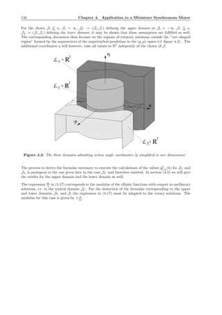
149. 4.2. Preliminary Discussion and Numerical Simulations 135
4.2 Preliminary Discussion and Numerical Simulations
In order to gain a first overview on the qualitative behaviour of (4.14) and its dependence on the parame-
ters, we present a list of results found through numerical simulations of system (4.14). These simulations
were carried out using the dstool–software package [3].
4.2.1 The Role of the Coupling and the Parameters ̺, m
Let us rewrite system (4.14) in the slightly more general form
˙q = p
˙p = −
a
2
2
sin(q) + µ ε (η1 cos(q + t) − η2 sin(q + t)) − ε2
̺ (p + 1) − ε2
m
˙η1 = −η1 + µ ε sin(q + t)
˙η2 = −η2 − 2 η3 + µ ε cos(q + t)
˙η3 = η2 − µ ε cos(q + t)
(4.23)
i.e. by introducing an additional parameter µ which enables us to control the amount of coupling be-
tween the two subsytems of the (q, p) and the η–coordinates. Considering the (q, p)–plane of the phase
space solely, system (4.23) then may be studied for special choices of the parameters µ, ̺ and m. The
corresponding phase portraits are depicted in figure 4.3. The parameter a is fixed to a = 2.33.
● ●
●
ρ
m
µ
●
Figure 4.3: Dependence of the phase portrait of (4.23) on the parameters

150. 136 Chapter 4. Application to a Miniature Synchronous Motor
1. µ = 0, ̺ = 0, m = 0 :
In this case the system considered is given by
˙q = p
˙p = −
a
2
2
sin(q)
hence the standard mathematical pendulum equation. This system is Hamiltonian and the separa-
trices cross the p–axis at p = ±a.
2. µ = 0, ̺ = 0, m = 0 :
The system considered is given by
˙q = p
˙p = −
a
2
2
sin(q) − ε2
m
corresponding to the equation of a mathematical pendulum with a small external torque. This
system is Hamiltonian as well.
3. µ = 0, ̺ = 0, m = 0 :
Then
˙q = p
˙p = −
a
2
2
sin(q) − ε2
̺ (p + 1)
corresponding to the equation of a mathematical pendulum with small constant damping and
external torque. This system is dissipative for ̺ > 0.
4. µ = 0, ̺ = 0, m = 0 :
In this last case we have
˙q = p
˙p = −
a
2
2
sin(q) + µ ε (η1 cos(q + t) − η2 sin(q + t))
˙η1 = −η1 + µ ε sin(q + t)
˙η2 = −η2 − 2 η3 + µ ε cos(q + t)
˙η3 = η2 − µ ε cos(q + t)
corresponding to the mathematical pendulum with a weak coupling to the η system. This system
is non–autonomous and numerical simulation yields a phase portrait which suggest an attractive
periodic solution close to the origin. (Note that q = p = 0, η = 0 does not solve the system).

151. 4.2. Preliminary Discussion and Numerical Simulations 137
4.2.2 The Role of the Parameter a
In order to obtain a first overwiew on the qualitative behaviour of (4.14), (4.23) respectively and in
particular the effect that the coupling of the two subsystems takes, we set ̺ = 0, m = 0 (and µ = 1).
For the parameter a we consider a = 0.54 and a = 20.38, i.e. the lower and upper bound of the domain
considered in (4.14). Since a = 4.0 corresponds to a resonant case (where GA 1.1a is not satisfied, see
section 4.1.4), we consider the value a = 4.1 in addition.
For each choice of the parameter a we depict the following plots: For the solutions (q, p)(t) of (4.14)
considered, the transformation (1.15) into the periodic solution (ˇq, ˇp, ˇη)(t, ε) and hence into the ( ˇQ, ˇP)–
coordinates is approximated numerically. Then the graph of the function t → H(( ˇQ, ˇP)(t)) is shown in a
first figure. The next figure shows the projections of the phase portrait onto the (q, p)–plane. The orbits
of a few solutions are shown near the eye–shaped region. Then the same trajectories are shown with a
large zoom out on the q–axis. This makes it possible to track solutions more globally and to observe the
long time behaviour.
For a = 0.54 the final figure shows a view on the (p, η2)–plane in order to illustrate the behaviour in the
η–space and to demonstrate how solutions approach η ≈ 0. This figure is very similar for a = 4.1 and
a = 20.38 and therefore omitted for these parameters.
Note that due to extreme zoom out, the trajectories plotted may be too tight to be distinguished and
seemingly fill an entire area.
a = 0.54, ̺ = 0, m = 0, (ε = 0.05)
real–world initial values: We first simulate the behaviour of the synchronous motor when switched on.
The corresponding initial values are refered to as the real–world initial values. For a = 0.54 we choose
eight equidistant values for ϑ(0) ∈ [−π, π], d
dτ ϑ(0) = 0 and transform them in accordance to lemma 4.1.2.
The corresponding trajectories then are plotted in black.
As visible in figure 4.4 they limit towards p = −1 which corresponds to d
dt ϑ = 0. The η–components
of these solutions approach a small neighbourhood of η = 0 after some transient behaviour. The corre-
sponding trajectories are shown in figure 4.5. This plot illustrates the existence of an attractive invariant
manifold close to η = 0, as expected by the results found in chapter 1.
We conclude that the power circuit enters some periodic behaviour (cf. transformations (4.6), (4.10)) but
the rotor does not start rotating when the motor is switched on. In figure 4.6 we see that H( ˇQ, ˇP) is
strictly bounded away from zero. As H = 0 is equivalent to ( ˇQ, ˇP) = 0 (modulo 2π in ˇQ) this shows
again that the solutions with real–world initial values remain O(1) away from the periodic solution of
(4.14), i.e. the synchronous rotary behaviour.
reduced system: Secondly we consider initial values with η = 0, i.e. close to the attractive invariant
manifold. This yields a more extensive view of the reduced system. More precisely we show trajectories
corresponding to q(0) = 0, η(0) = 0 and p(0) ∈ [−2, 2]. These trajectories are plotted in grey. The
following result may be seen in figure 4.7 and figure 4.8 best:
For p(0) −0.54 the orbits limit in p = −1. For −0.54 p(0) 0.54 the orbits are caught by the
periodic solution close to the origin (refer also to figure 4.6 where H(( ˇQ, ˇP)(t)) → 0). For p(0) 0.54
some solutions are caught by this periodic solution as well, other solutions pass the q–axis and limit in
p = −1.

152. 138 Chapter 4. Application to a Miniature Synchronous Motor
t
p
Figure 4.4: t ∈ [0, 2000], p ∈ [−2, 2]
η
p
2
Figure 4.5: p ∈ [−2, 2], η2 ∈ [−2, 2]

153. 4.2. Preliminary Discussion and Numerical Simulations 139
H(Q,P)
t
Figure 4.6: t ∈ [0, 2000], H( ˇQ, ˇP) ∈ [0, 1]
q
p
p=-1
Figure 4.7: q ∈ [−4, 4], p ∈ [−2, 2]
q
p
Figure 4.8: q ∈ [−500, 500], p ∈ [−2, 2]

154. 140 Chapter 4. Application to a Miniature Synchronous Motor
a = 4.1, ̺ = 0, m = 0, (ε = 0.05)
real–world initial values: We consider solutions starting with three different values for ϑ(0). In order
to visualize the long time behaviour we have plotted the corresponding trajectories with time–dependent
colour. For t = 0 the orbits are light grey and become black as t → ∞. Two orbits corresponding
to ϑ(0) = −2 and ϑ(0) = −1.1 tend towards the periodic solution close to the origin within the time
0 ≤ t ≤ 2000 integrated numerically. A third orbit corresponding to ϑ(0) = −1.04 is plotted last and
covers the previous two trajectories. Due to some capture in a resonance it is caught in an attractor inside
the eye–shaped region (cf. section 4.5). This is seen in figure 4.11 as the orbit covers itself increasingly
the darker it becomes and the black part of the trajectory therefore corresponds to the ω–limit set. This
ω–limit set inside the attractor has the shape of a circle and intersects the p–axis at p ≈ 1.2.
reduced system: Trajectories corresponding to initial values with q(0) = 0, η(0) = 0 and p(0) ∈ [−6, 6]
are coloured in grey. All these orbits are attracted by the eye–shaped region eventually (figure 4.12).
This is seen in figure 4.10, too, as the energies H( ˇQ, ˇP) become less than 8 as t → ∞ and the set
ˇQ, ˇP H( ˇQ, ˇP) ≤ 8 lies within the eye–shaped region. The plot of H(( ˇQ, ˇP)(t)) versus t illustrates
the capture in the resonance as well: In figure 4.9 this function is evaluated for 20 solutions with initial
values p(0) ∈ [1, 3]. For three of these solutions the energy approaches the value ≈ 0.72 = H(0, 1.2)
indicating a capture in the resonance. (The same is visible for the solution with the real–world initial
value ϑ(0) = −1.04 in figure 4.10.)
H(Q,P)
t
Figure 4.9: t ∈ [0, 6000], H( ˇQ, ˇP) ∈ [0, 2]

155. 4.2. Preliminary Discussion and Numerical Simulations 141
H(Q,P)
t
Figure 4.10: t ∈ [0, 3000], H( ˇQ, ˇP) ∈ [0, 10]
q
p
p=-1
Figure 4.11: q ∈ [−4, 4], p ∈ [−6, 6]
q
p
Figure 4.12: q ∈ [−3000, 3000], p ∈ [−6, 6]

156. 142 Chapter 4. Application to a Miniature Synchronous Motor
In order to illustrate the ε–dependence of the amount of solutions being captured in the resonance
presumed, we plot q(t) over the values
σ = δ t + q(0)
for ten equidistant values q(0) ∈ [−3, −0.5] and three different choices for ε. The result is shown in
figure 4.13 where we have used different shades of grey for colouring and different values for δ according
to the following choices of ε:
black ε = 0.4, δ = 3 · 10−5
⇒ 5 orbits are caught in the resonance
dark grey ε = 0.2, δ = 2 · 10−5
(covers previous plot) ⇒ 3 orbits are caught in the resonance
light grey ε = 0.1, δ = 1 · 10−5
(covers previous plots) ⇒ 2 orbits are caught in the resonance.
σ
q
Figure 4.13: σ ∈ [−3, −0.5], q ∈ [−4, 4]
Hence the number of solutions captured in the resonance decreases as ε → 0. Note that the size of
the attracting periodic solution ˇq(t, ε) decreases as ε → 0 while the maximal q–values of the solutions
captured remains constant in the main as this corresponds to the ε–independent position of the resonance.
a = 20.38, ̺ = 0, m = 0, (ε = 0.1)
The colouring of the plots is processed as for a = 4.1, i.e. time–dependent for the real–world initial values
and grey for trajectories close to the reduced system.
real–world initial values: Since the solutions corresponding to this set of initial values start on the line
p = −1 most trajectories start within the eye–shaped region and are caught by the periodic solution near
the origin. The orbits starting outside the eye–shaped region perform a few shifts in the q–coordinate,
then drift into the eye–shaped region as well (see figure 4.16). No capture into resonance is found. As
the numerical integration is performed over the larger time scale t ∈ [0, 4000] and the orbits are coloured
darker with increasing time again, we see in figure 4.15 that the solutions tend slower towards the periodic
solution at the origin, i.e. the periodic solution is less attractive (compared to the preceeding case a = 4.1).
reduced system: The solutions with initial values corresponding to q(0) = 0, η(0) = 0 and p(0) ∈
[−30, 30] are attracted by the eye–shaped region, too.

157. 4.2. Preliminary Discussion and Numerical Simulations 143
H(Q,P)
t
Figure 4.14: t ∈ [0, 4000], H( ˇQ, ˇP) ∈ [0, 400]
q
p
p=-1
Figure 4.15: q ∈ [−4, 4], p ∈ [−30, 30]
q
p
Figure 4.16: q ∈ [−400, 400], p ∈ [−30, 30]

158. 144 Chapter 4. Application to a Miniature Synchronous Motor
4.3 Explicit Formulae for the Reduced System, Following Chap-
ter 1
The purpose of this section is to carry out the programme of chapter 1 in the specific case of (4.14). Based
on the general formulae for the system after each transformation (transformations were performed into
the periodic solution, the strongly stable manifold, into action angle coordinates and on the attractive
invariant manifold) we eventually will obtain explicit representations of the maps gj
k,n as in lemma 1.6.9.
Although the formulae given in chapter 1 enable the computation of gj
k,n for j = 2 and j = 3, we will
deal with the ε2
–terms only. This will be sufficient to discuss the model under investigation.
4.3.1 The Transformation into the Periodic Solution
Recall the results given in proposition 1.2.4 : For the map F as in (4.1.3) it follows from (4.19)–(4.22)
that (1.18) takes the form
ˇF1
( ˇQ, ˇP, H, t) = ei ˇQ
M H eit
+ e−i ˇQ
M H e−it
(4.24)
ˇF2
( ˇQ, ˇP, H, t) = −
0
̺ ˇP + (m + ̺)
+ ∆(0, ˇQ, ˇP)
0
(m + ̺)
+ e−i ˇQ
M − ∆(−2, ˇQ, ˇP) M α1,1
−1,2 e−i2t
+ e−i ˇQ
M − ∆(0, ˇQ, ˇP) M α1,1
1,2
+ ei ˇQ
M − ∆(0, ˇQ, ˇP) M α1,1
−1,2
+ ei ˇQ
M − ∆(2, ˇQ, ˇP) M α1,1
1,2 ei2t
(4.25)
ˇG1
( ˇQ, ˇP, t) = ei ˇQ
− 1 v eit
+ e−i ˇQ
− 1 ¯v e−it
(4.26)
where
α1,1
1,2 = [i IR3 − A]−1
v α1,1
−1,2 = [−i IR3 − A]−1
¯v.
Defining
B0 :=
0 1
0 0
B1 := B−1 :=
0 0
−a2
8 0
. (4.27)
we write JD2
H( ˇQ, ˇP) =
0 1
− a
2
2
cos( ˇQ) 0
in the form
JD2
H( ˇQ, ˇP) = B0 + ei ˇQ
B1 + e−i ˇQ
B−1
which implies
∆(n, ˇQ, ˇP) = i n IC 2 − JD2
H( ˇQ, ˇP) i n IC 2 − JD2
H(0, 0)
−1
= ∆0(n) + ∆1(n) ei ˇQ
+ ∆−1(n) e−i ˇQ
(4.28)

159. 4.3. Explicit Formulae for the Reduced System, Following Chapter 1 145
where
∆0(n) := i n IC 2 − B0] [i n IC 2 − B0 − B1 − B−1]
−1
∆1(n) := −B1 [i n IC 2 − B0 − B1 − B−1]−1
∆−1(n) := −B−1 [i n IC 2 − B0 − B1 − B−1]−1
.
Using these abbreviations we rewrite (4.25) as
ˇF2
( ˇQ, ˇP, H, t) = −̺
0
ˇP
− (m + ̺) IC 2 − ∆(0, ˇQ, ˇP)
0
1
+ ˜z0
0 + ˜z+
0 ei ˇQ
+ ˜z−
0 e−i ˇQ
+ ˜z0
2 + ˜z+
2 ei ˇQ
+ ˜z−
2 e−i ˇQ
ei2t
+ ˜z0
−2 + ˜z+
−2 ei ˇQ
+ ˜z−
−2 e−i ˇQ
e−i2t
(4.29)
with
˜z0
2 = −∆0(2) M α1,1
1,2, ˜z0
−2 = −∆0(−2) M α1,1
−1,2
˜z+
2 = (IC 2 − ∆1(2)) M α1,1
1,2, ˜z+
−2 = −∆1(−2) M α1,1
−1,2
˜z−
2 = −∆−1(2) M α1,1
1,2, ˜z−
−2 = (IC 2 − ∆−1(−2)) M α1,1
−1,2
˜z0
0 = −∆0(0) M α1,1
1,2 − ∆0(0) M α1,1
−1,2
˜z+
0 = (IC 2 − ∆1(0)) M α1,1
−1,2 − ∆1(0) M α1,1
1,2
˜z−
0 = (IC 2 − ∆−1(0)) M α1,1
1,2 − ∆−1(0) M α1,1
−1,2.
Computations in Maple [15] yield the following results :
α1,1
1,2 := −
1
4
−
1
4
i
3
4
−
1
4
i −
1
4
−
1
4
i
T
α1,1
−1,2 := −
1
4
+
1
4
i
3
4
+
1
4
i −
1
4
+
1
4
i
T
IC 2 − ∆(0, ˇQ, ˇP)
0
1
=
0
1 − cos( ˇQ)
˜z0
2 := 0 4
i
−16 + a2
T
˜z0
−2 := 0 − 4
i
−16 + a2
T
˜z+
2 := 0
1
4
i −
1
8
i a2
−16 + a2
T
˜z−
−2 := 0 −
1
4
i +
1
8
i a2
−16 + a2
T
˜z+
−2 := 0
1
8
i a2
−16 + a2
T
˜z−
2 := 0 −
1
8
i a2
−16 + a2
T

160. 146 Chapter 4. Application to a Miniature Synchronous Motor
˜z0
0 := [ 0 0 ]T
˜z+
0 := 0
1
2
i
T
˜z−
0 := 0 −
1
2
i
T
4.3.2 The Transformation into the Strongly Stable Manifold
In this section we refer to the statement given in proposition 1.4.9. In accordance with (4.24)–(4.30) we
apply (1.90) (note that ˆF2
is evaluated for H = 0):
ˆF1
(Q, P, H, t) = eiQ
− 1 B1 + e−iQ
− 1 B−1 V1
(t) H
+ eiQ
− 1 M H eit
+ e−iQ
− 1 M H e−it
(4.30)
ˆF2
(Q, P, 0, t) = −̺
0
P
− (m + ̺)
0
1 − cos(Q)
+ ˜z0
0 + ˜z+
0 eiQ
+ ˜z−
0 e−iQ
+ ˜z0
2 + ˜z+
2 eiQ
+ ˜z−
2 e−iQ
ei2t
+ ˜z0
−2 + ˜z+
−2 eiQ
+ ˜z−
−2 e−iQ
e−i2t
− V1
(t) eiQ
− 1 v eit
+ e−iQ
− 1 ¯v e−it
.
(4.31)
From (1.91) together with (4.26) we deduce
ˆG1
(Q, P, H, t) = eiQ
− 1 v eit
+ e−iQ
− 1 ¯v e−it
. (4.32)
It remains to compute the linear map V1
(t). We therefore consider the decomposition
esA
=
3
j=1
esλj
TA,λj e−sB
=
2
k=1
e−sωk
TB,ωk
implied by (1.82), where
λ1 := −1, λ2 := −1
2 + i
√
7
2 , λ3 := −1
2 − i
√
7
2 ω1 := i
a
2
, ω2 := −i
a
2
and
TA,λ1 :=


1 0 0
0 0 0
0 0 0


TA,λ2 :=





0 0 0
0
1
14
i
√
7 +
1
2
2
7
i
√
7
0 −
1
7
i
√
7 −
1
14
i
√
7 +
1
2





TA,λ3 :=





0 0 0
0 −
1
14
i
√
7 +
1
2
−
2
7
i
√
7
0
1
7
i
√
7
1
14
i
√
7 +
1
2





TB,ω1 :=



1
2
−
i
a
1
4
i a
1
2


 TB,ω2 :=



1
2
i
a
−
1
4
i a
1
2




161. 4.3. Explicit Formulae for the Reduced System, Following Chapter 1 147
Taking into account (4.24) which implies ∂H
ˇF1
(0, 0, 0, t) = M eit
+ M e−it
, hence ∂H
ˇF1
1 (0, 0, 0, t) = M,
∂H
ˇF1
−1(0, 0, 0, t) = M, we determine V1
(t) in agreement with (1.83), (1.84):
V1
(t) = eit
V1
1 + e−it
V1
−1 (4.33)
where
V1
1 =
3
j=1
2
k=1
(i − ωk + λj)−1
TB,ωk
M TA,λj
V1
−1 =
3
j=1
2
k=1
(−i − ωk + λj)−1
TB,ωk
M TA,λj .
Evaluation of these sums using Maple [15] yields
V1
1 :=




2
−8 i + a2
−24 i + 2 i a2
−32 i − 20 a2 − 8 i a2 + a4
−32 − 16 i
−32 i − 20 a2 − 8 i a2 + a4
−2 + 2 i
−8 i + a2
8 i − 2 i a2
− 8 − 2 a2
−32 i − 20 a2 − 8 i a2 + a4
−4 i a2
+ 16 i + 16
−32 i − 20 a2 − 8 i a2 + a4




V1
−1 :=




2
8 i + a2
24 i − 2 i a2
32 i − 20 a2 + 8 i a2 + a4
−32 + 16 i
32 i − 20 a2 + 8 i a2 + a4
−2 − 2 i
8 i + a2
−8 i + 2 i a2
− 8 − 2 a2
32 i − 20 a2 + 8 i a2 + a4
4 i a2
− 16 i + 16
32 i − 20 a2 + 8 i a2 + a4



 .
Plugging (4.33) into (4.30), (4.31) we obtain a representation for ˆF1
(Q, P, H, t) and ˆF2
(Q, P, H, t) which
is more convenient for the further process:
ˆF1
(Q, P, H, t) = ζ+
1 eiQ
− 1 + ζ−
1 e−iQ
− 1 H eit
+ ζ+
−1 eiQ
− 1 + ζ−
−1 e−iQ
− 1 H e−it
(4.34)
with
ζ+
1 = B1 V1
1 + M ζ−
−1 = B−1 V1
−1 + M
ζ+
−1 = B1 V1
−1 ζ−
1 = B−1 V1
1
and
ˆF2
(Q, P, 0, t) = −̺
0
P
− (m + ̺)
0
1 − cos(Q)
+ z0
0 + z+
0 eiQ
+ z−
0 e−iQ
+ z0
2 + z+
2 eiQ
+ z−
2 e−iQ
ei2t
+ z0
−2 + z+
−2 eiQ
+ z−
−2 e−iQ
e−i2t
(4.35)
where
z0
0 = ˜z0
0 + V1
1 ¯v + V1
−1 v
z+
0 = ˜z+
0 − V1
−1 v
z−
0 = ˜z−
0 − V1
1 ¯v
z0
2 = ˜z0
2 + V1
1 v z0
−2 = ˜z0
−2 + V1
−1 ¯v
z+
2 = ˜z+
2 − V1
1 v z−
−2 = ˜z−
−2 − V1
−1 ¯v
z−
2 = ˜z−
2 z+
−2 = ˜z+
−2.

162. 148 Chapter 4. Application to a Miniature Synchronous Motor
The corresponding explicit formulae are as follows :
ζ+
1 :=



0 0 0
a2
− 16 i
−32 i + 4 a2
−28 i a2
+ i a4
+ 64 + 16 a2
−128 i − 80 a2 − 32 i a2 + 4 a4
4 a2
+ 2 i a2
−32 i − 20 a2 − 8 i a2 + a4



ζ−
−1 :=



0 0 0
a2
+ 16 i
32 i + 4 a2
28 i a2
− i a4
+ 64 + 16 a2
128 i − 80 a2 + 32 i a2 + 4 a4
4 a2
− 2 i a2
32 i − 20 a2 + 8 i a2 + a4



ζ+
−1 :=



0 0 0
−
a2
32 i + 4 a2
−12 i a2
+ i a4
128 i − 80 a2 + 32 i a2 + 4 a4
4 a2
− 2 i a2
32 i − 20 a2 + 8 i a2 + a4



ζ−
1 :=



0 0 0
a2
−32 i + 4 a2
12 i a2
− i a4
−128 i − 80 a2 − 32 i a2 + 4 a4
4 a2
+ 2 i a2
−32 i − 20 a2 − 8 i a2 + a4



z0
0 := −49152 a2
−6144 a4
32768 a2−40 a10+65536+a12+30720 a4−2048 a6+528 a8
32768+36864 a2
−4 a10
−1216 a6
+6656 a4
+96 a8
32768 a2−40 a10+65536+a12+30720 a4−2048 a6+528 a8
z+
0 := −24 i a2
−32 a2
+2 i a4
−128 i
−256−128 i a2−20 a4−64 a2+16 i a4+a6
128+112 a2
−20 i a4
−12 a4
+i a6
−512−256 i a2−40 a4−128 a2+32 i a4+2 a6
z−
0 := 24 i a2
−32 a2
−2 i a4
+128 i
−256+128 i a2−20 a4−64 a2−16 i a4+a6
128+112 a2
+20 i a4
−12 a4
−i a6
−512+256 i a2−40 a4−128 a2−32 i a4+2 a6
z0
2 := 16 i a2
+16 a2
−64−128 i
−256+128 i a2−20 a4−64 a2−16 i a4+a6
−256 a2
−136 i a4
+192 i a2
−2048 i+48 a4
+6 i a6
4096−2048 i a2+768 a2+384 i a4+256 a4−36 a6−16 i a6+a8
z0
−2 := −16 i a2
+16 a2
−64+128 i
−256−128 i a2−20 a4−64 a2+16 i a4+a6
−256 a2
+136 i a4
−192 i a2
+2048 i+48 a4
−6 i a6
4096+2048 i a2+768 a2−384 i a4+256 a4−36 a6+16 i a6+a8
z+
2 := 64−16 i a2
+128 i−16 a2
−256+128 i a2−20 a4−64 a2−16 i a4+a6
i a8
+2048 a2
+1024 i a4
−1792 i a2
+16384 i−512 a4
+16 a6
−68 i a6
32768−16384 i a2+6144 a2+3072 i a4+2048 a4−288 a6−128 i a6+8 a8
z−
−2 := 16 i a2
−16 a2
+64−128 i
−256−128 i a2−20 a4−64 a2+16 i a4+a6
−i a8
+2048 a2
−1024 i a4
+1792 i a2
−16384 i−512 a4
+16 a6
+68 i a6
32768+16384 i a2+6144 a2−3072 i a4+2048 a4−288 a6+128 i a6+8 a8
z−
2 := 0 −
i a2
−128 + 8 a2
z+
−2 := 0
i a2
−128 + 8 a2
4.3.3 The Transformation into Action Angle Coordinates
As mentioned above, the aim of this section 4.3 is to derive explicit formulae for the maps g2
k,n which
appear in the equation for the action variable h of the restricted system (cf. (1.158)). Considering the
definition of these maps g2
k,n via (1.156), i.e.
g2
k,n(h) =
k1,k2∈Z
k1+k2=k
|n1|≤N,|n2|≤2N
n1+n2=n
F1,1
k1,n1,3(h) S1
k2,n2
(h) + F2,0
k,n,3(h)
(4.36)
we see that we need to compute the maps F1,1
k1,n1,3, S1
k2,n2
(h) and F2,0
k1,n1,3. In this subsection we aim
on explicit formulae for F1,1
k1,n1,3 and F2,0
k1,n1,3. The computation of the quantities S1
k,n is related to the
calculation of the attractive invariant manifold, which we postpone until the next subsection. However
we will prepare these computations as well, giving some formulae for G1,0
k,n. Note that by consequence of
remark 1.6.11 we have g1
k,n(h) = 0 for all h ∈ R as the map F1
considered here vanishes for η = 0.
Recall that by (1.98)
Φ(ϕ, h) := (˜q, ˜p)(ϕ, P(h)) := (q, p)( ϕ
Ω(P(h)) ; 0, P(h)) (4.37)

163. 4.3. Explicit Formulae for the Reduced System, Following Chapter 1 149
where (q, p)(t; 0, p0) are the solutions of (4.16) given by (4.17). Using (4.34) and (4.35) derived above
definition 1.6.5 yields
F1,1
3 (t, ϕ, h)H =
1
d
dh H(0,P(h))
∇H(Φ(ϕ, h)) ζ+
1 ei˜q(ϕ,P(h))
− 1 + ζ−
1 e−i˜q(ϕ,P(h))
− 1 H eit
+ 1
d
dh H(0,P(h))
∇H(Φ(ϕ, h)) ζ+
−1 ei˜q(ϕ,P(h))
− 1 + ζ−
−1 e−i˜q(ϕ,P(h))
− 1 H e−it
(4.38)
F2,0
3 (t, ϕ, h) = − ̺ 1
d
dh H(0,P(h))
∇H(Φ(ϕ, h))
0
˜p(ϕ, P(h))
− (m + ̺) 1
d
dh H(0,P(h))
∇H(Φ(ϕ, h))
0
1 − ei˜q(ϕ,P(h))
+ e−i˜q(ϕ,P(h))
/2
+ 1
d
dh H(0,P(h))
∇H(Φ(ϕ, h)) z0
0 + z+
0 ei˜q(ϕ,P(h))
+ z−
0 e−i˜q(ϕ,P(h))
+ 1
d
dh H(0,P(h))
∇H(Φ(ϕ, h)) z0
2 + z+
2 ei˜q(ϕ,P(h))
+ z−
2 e−i˜q(ϕ,P(h))
ei2t
+ 1
d
dh H(0,P(h))
∇H(Φ(ϕ, h)) z0
−2 + z+
−2 ei˜q(ϕ,P(h))
+ z−
−2 e−i˜q(ϕ,P(h))
e−i2t
.
(4.39)
The analogous result may be obtained for G1,0
k,n from (4.26), (1.138) and (1.143)
G1,0
(t, ϕ, h) = ei˜q(ϕ,P(h))
− 1 v eit
+ e−i˜q(ϕ,P(h))
− 1 ¯v e−it
. (4.40)
In a next step we introduce some Fourier series which will enable us to express F1,0
3 , F2,0
3 and G1,0
in
accordance with (1.142), (1.143).
Let (ak)k∈Z, (bk)k∈Z, (αk)k∈Z, (βk)k∈Z, (αβk)k∈Z, (aβk)k∈Z and (bβk)k∈Z be the unique sequences of
maps defined on R, such that
ei˜q(ϕ,P(h))
=
k∈Z
ak(h) eikϕ
˜p(ϕ, P(h)) =
k∈Z
bk(h) eikϕ
ei˜q(ϕ,P(h))
− 1 =
k∈Z
αk(h) eikϕ
∇H(Φ(ϕ, h)) =
k∈Z
βk(h) eikϕ
(4.41)
ei˜q(ϕ,P(h))
− 1 ∇H(Φ(ϕ, h)) =
k∈Z
αβk(h) eikϕ
ei˜q(ϕ,P(h))
∇H(Φ(ϕ, h)) =
k∈Z
aβk(h) eikϕ
˜p(ϕ, P(h)) ∇H(Φ(ϕ, h)) =
k∈Z
bβk(h) eikϕ
hold for all h, ϕ ∈ R. Note that ak(h), bk(h), αk(h) ∈ C, while βk(h), αβk(h), aβk(h), bβk(h) ∈ C2
.
Moreover we use double letters to denote the quantities αβ, aβ which may be unconventional for the
reader. However, we will see in what follows that these sequences may be represented as the convolution of
two sequences (in fact the sequences (αk)k∈Z, (βk)k∈Z and (ak)k∈Z, (βk)k∈Z, respectively). This justifies
the special notation.

164. 150 Chapter 4. Application to a Miniature Synchronous Motor
Taking the complex conjugate of (4.3.3) it is evident that
e−i˜q(ϕ,P(h))
− 1 =
k∈Z
αk(h)e−ikϕ
e−i˜q(ϕ,P(h))
− 1 ∇H(Φ(ϕ, h)) =
k∈Z
αβk(h)e−ikϕ
e−i˜q(ϕ,P(h))
∇H(Φ(ϕ, h)) =
k∈Z
aβk(h)e−ikϕ
.
With the help of these representations we now are in the position to rewrite (4.38)–(4.40) as follows:
F1,1
3 (t, ϕ, h)H := 1
d
dh H(0,P(h))
k∈Z
αβk(h) eikϕ
ζ+
1 H +
k∈Z
αβk(h)e−ikϕ
ζ−
1 H eit
+ 1
d
dh H(0,P(h))
k∈Z
αβk(h) eikϕ
ζ+
−1 H +
k∈Z
αβk(h)e−ikϕ
ζ−
−1 H e−it
hence in correspondance with (1.142)
F1,1
k,1,3(h) H = 1
d
dh H(0,P(h))
αβk(h)| ζ+
1 H + αβ−k(h) ζ−
1 H
F1,1
−k,−1,3(h) H = 1
d
dh H(0,P(h))
αβ−k(h) ζ+
−1 H + αβk(h) ζ−
−1 H
F1,0
k1,n1,3 = 0 else.
(4.42)
In much the same way we find
F2,0
3 (t, ϕ, h) := −̺ 1
d
dh H(0,P(h))
k∈Z
bβk(h) eikϕ 0
1
−(m + ̺) 1
d
dh H(0,P(h))
k∈Z
βk(h) eikϕ 0
1
−
k∈Z
aβk(h) eikϕ 0
1
2
−
k∈Z
aβk(h)e−ikϕ 0
1
2
+ 1
d
dh H(0,P(h))
k∈Z
βk(h) eikϕ
z0
0 +
k∈Z
aβk(h) eikϕ
z+
0 +
k∈Z
aβk(h)e−ikϕ
z−
0
+ 1
d
dh H(0,P(h))
k∈Z
βk(h) eikϕ
z0
2 +
k∈Z
aβk(h) eikϕ
z+
2 +
k∈Z
aβk(h)e−ikϕ
z−
2 ei2t
+ 1
d
dh H(0,P(h))
k∈Z
βk(h) eikϕ
z0
−2 +
k∈Z
aβk(h) eikϕ
z+
−2 +
k∈Z
aβk(h)e−ikϕ
z−
−2 e−i2t

165. 4.3. Explicit Formulae for the Reduced System, Following Chapter 1 151
hence
F2,0
k,2,3(h) = 1
d
dh H(0,P(h))
βk(h)| z0
2 + aβk(h)| z+
2 + aβ−k(h) z−
2
F2,0
−k,−2,3(h) = 1
d
dh H(0,P(h))
β−k(h)| z0
−2 + aβ−k(h) z+
−2 + aβk(h) z−
−2
F2,0
k,0,3(h) = 1
d
dh H(0,P(h))
βk(h)| z0
0 + aβk(h)| z+
0 + aβ−k(h) z−
0
− ̺ bβk(h)
0
1
− (m + ̺) βk(h)
0
1
− aβk(h) + aβ−k(h)
0
1
2
F2,0
k,n(h) = 0 else.
(4.43)
Finally (4.40) and (4.3.3) imply
G1,0
(t, ϕ, h) =
k∈Z
αk(h) v ei(kϕ+t)
+
k∈Z
αk(h) ¯v e−i(kϕ+t)
. (4.44)

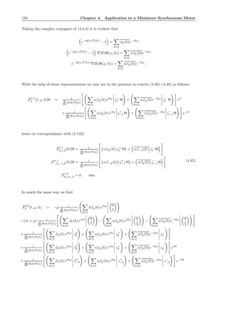
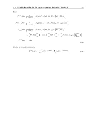
166. 152 Chapter 4. Application to a Miniature Synchronous Motor
4.3.4 The Attractive Invariant Manifold
Using the results found in proposition 1.6.7 together with (4.44) we can immediately write down the
explicit formula for the coefficient maps Sj
k,n :
S1
k,1(h) = [i(k ω(h) + 1)IR3 − A]
−1
αk(h) v
S1
−k,−1(h) = [i(−k ω(h) − 1)IR3 − A]
−1
αk(h) ¯v
S1
k,n(h) = 0 if |n| = 1
(4.45)
where ω(h) = Ω(P(h)) (cf. (1.99)). As mentioned in the introduction of section 4.3.3 we may confine
ourselves to the explicit computation of these coefficients.
In what follows we will list the Maple [15] –procedures corresponding to the quantities discussed in
order to enable the reader to reproduce the results found here. We start with the procedure used to
define S1
k,1, S1
−k,−1 (for |k| smaller than a given integer M):
S1_build := proc(kappa,alpha,alphacc)
local k,SS;
global Omega,M,v,vb,a;
SS[1] := table([seq(k = scalarmul(multiply(inverse(scalarmul(Id3,
I*(k*Omega(kappa,a)+1))-A),v),alpha[k]),k = -M .. M)]);
SS[-1] := table([seq(-k = scalarmul(multiply(inverse(scalarmul(Id3,
I*(-k*Omega(kappa,a)-1))-A),vb),alphacc[k]),k = -M .. M)]);
table([seq((k,-1) = evalm(SS[-1][k]),k = -M .. M),seq((k,1) = evalm(SS[1][k]),
k = -M .. M)])
end
(The variable ”kappa” will be defined in definition 4.3.2. The expression ”alphacc” symbolizes the
conjugate complex of ”alpha”.)

167. 4.3. Explicit Formulae for the Reduced System, Following Chapter 1 153
4.3.5 Main Result of Section 4.3
Combining the results derived in the preceding two subsections we now are in the position to evaluate
the formula given in (4.38) for g2
k,n. We will see that due to the theory deduced in chapter 2 we may
restrict ourselves to the cases where (k, n) = (0, 0) or n < 0 < k.
In a first step we collect the terms in (4.43)–(4.45) which contribute to the sum appearing in (4.36) for
(k, n) = (0, 0):
g2
0,0(h) =
k∈Z
F1,1
k,n,3(h) S1
−k,−1(h) + F1,1
−k,−n,3(h) S1
k,1(h) + F2,0
0,0,3(h)
= 1
d
dh H(0,P(h))
k∈Z
αβk(h)| ζ+
1 S1
−k,−1(h) + αβ−k(h) ζ−
1 S1
−k,−1(h)
+ αβ−k(h) ζ+
−1 S1
k,1(h) + αβk(h) ζ−
−1 S1
k,1(h)
+ β0(h)| z0
0 + aβ0(h)| z+
0 + αβ0(h) z−
0
− ̺ bβ0(h)
0
1
− (m + ̺) β0(h)
0
1
− aβ0(h) + aβ0(h)
0
1
2
. (4.46)
evalG00 := proc(beta, alphabeta, abeta, bbeta, alphabetacc, abetacc, bbetacc, zeta, z, S)
local G00, k;
global apar, M, cutoff, rho, m;
G00 := 0;
for k from -M to M do
G00 := G00
+ evalf(dotprod(alphabeta[k], multiply(zeta[1][1], S[-k, -1]),’orthogonal’))
+ evalf(dotprod(alphabetacc[-k],multiply(zeta[-1][1], S[-k, -1]), ’orthogonal’))
+ evalf(dotprod(alphabeta[-k], multiply(zeta[1][-1], S[k, 1]),’orthogonal’))
+ evalf(dotprod(alphabetacc[k],multiply(zeta[-1][-1], S[k, 1]), ’orthogonal’))
od;
G00 := G00 + normal(dotprod(beta[0], z[0][0], ’orthogonal’), expanded)
+ normal(dotprod(abeta[0], z[1][0], ’orthogonal’),expanded)
+ normal(dotprod(abetacc[0], z[-1][0], ’orthogonal’), expanded);
G00 := G00 - rho*normal(dotprod(bbeta[0], vector([0, 1]), ’orthogonal’), expanded);
G00 := G00 - (m + rho)*normal(dotprod( evalm(beta[0] - 1/2*abeta[0] - 1/2*abetacc[0]),
vector([0, .5]), ’orthogonal’), expanded);
if abs(Im(G00)) < cutoff then G00 := evalc(Re(G00))
else print(‘## E R R O R : ## cutoff too small in evalG00(..) : Im(G00)=‘, Im(G00))
fi;
G00
end

168. 154 Chapter 4. Application to a Miniature Synchronous Motor
Carrying out the same step in the case when k = 0, n < 0, one gets the following expression:
g2
−k,−2(h) =
k1,k2∈Z
k1+k2=k
F1,1
−k1,−1,3(h) S1
−k2,−1(h) + F2,0
−k,−2,3(h)
= 1
d
dh H(0,P(h))
k1,k2∈Z
k1+k2=k
αβ−k1
(h) ζ+
−1 S1
−k2,−1(h) + αβk1
(h) ζ−
−1 S1
−k2,−1(h)
+ β−k(h)| z0
−2 + aβ−k(h) z+
−2 + αβk(h) z−
−2 (4.47)
and g2
k,n = 0 if n < 0 and n = −2.
evalGk2 := proc(k, beta, alphabeta, abeta, alphabetacc, abetacc, zeta, z, S)
local Gk2, k1, k2;
global M, cutoff;
Gk2 := 0;
for k1 from -M to M do
for k2 from -M to M do
if k1 + k2 = k then
Gk2 := Gk2
+ evalf(dotprod(alphabeta[-k1], evalm(multiply(zeta[1][-1],S[-k2, -1])),
’orthogonal’));
+ evalf(dotprod(alphabetacc[k1], evalm(multiply(zeta[-1][-1],S[-k2, -1])),
’orthogonal’))
fi
od;
od;
Gk2 := Gk2 + normal(dotprod(beta[-k], z[0][-2], ’orthogonal’), expanded);
Gk2 := Gk2 + normal(dotprod(abeta[-k], z[1][-2], ’orthogonal’), expanded);
Gk2 := Gk2 + normal(dotprod(abetacc[k], z[-1][-2], ’orthogonal’), expanded);
2*abs(Gk2)
end

169. 4.3. Explicit Formulae for the Reduced System, Following Chapter 1 155
4.3.6 The Calculation of the Fourier Coefficients
We have seen in the preceeding chapters that the maps g2
0,0 and g2
km,−2 play a crucial role in the analysis
of the system under investigation. In order to apply the results derived there we need more information
about the properties of these maps g2
0,0 and g2
−k,−2. Due to the complexity of the explicit formulae (4.46)
and (4.47) we will gain this information by approximating these expressions numerically. Aiming on such
numerical evaluations it is necessary to find a way to compute the values βk(h), αβk(h), aβk(h) and
bβk(h) arising in (4.46) and (4.47). This is the purpose of this last subsection. As we will deal with
various sequences of Fourier–coefficients in what follows, we introduce the following notation.
Definition 4.3.1 The convolution x = (xk)k∈Z of the sequences y = (yk)k∈Z, z = (zk)k∈Z (where yk ∈ C
and zk ∈ Cn
, n ∈ N∗
) is defined as follows:
x = y ∗ z :=




k1,k2∈Z
k1+k2=k
yk1 zk2




k∈Z
. (4.48)
With the help of convolutions it will be possible to express the maps βk(h), αβk(h), aβk(h) and bβk(h)
in an easy way. Let us therefore introduce the following sequences:
Definition 4.3.2 In accordance with the notation found in [2] we introduce the following abbreviations
κ(h) :=
P(h)
a
q(h) := e−π
K(
√
1−κ(h)2
)
K(κ(h)) (4.49)
and define then sequences dn(h) = (dn(h)k)k∈Z, iκsn(h) = (iκsn(h)k)k∈Z and cn(h) = (cn(h)k)k∈Z by
dn(h)k =



π
K(κ(h))
q(h)|k|/2
1 + q(h)|k|
if k even
0 else
iκsn(h)k =



sgn(k)
π
K(κ(h))
q(h)|k|/2
1 − q(h)|k|
if k odd
0 else
cn(h)k =



π
κ(h) K(κ(h))
q(h)|k|/2
1 + q(h)|k|
if k odd
0 else
.
(4.50)
Note that considering the central domain, i.e. J = JC the limit h → ∞ corresponds to P(h) → a hence
κ → 1. If we consider regions in JC close to the border LJr we therefore focus on values κ 1. On
the other hand this border LJr is close to the separatrices of the unperturbed pendulum (cf. figure 1.2).
Hence the values κ 1 correspond to regions close to the separatrices. This is true for the cases J = JL
and J = JU as well.

170. 156 Chapter 4. Application to a Miniature Synchronous Motor
K := LegendreKc q := ( κ, pot ) → e
−
pot π LegendreKc1( κ )
LegendreKc( κ )
Ω := ( κ, a ) → evalf
1
4
π a
K( κ )
dn_build := proc(kappa)
local k,dn;
global K,q,M;
dn := table([seq(k = 0,k = -M .. M)]);
for k from -M to M do
if type(k,even) then
dn[k] := evalf(Pi/K(kappa)*q(kappa,1/2*abs(k))/(1+q(kappa,abs(k))))
fi
od;
table([seq(k = dn[k],k = -M .. M)])
end
iksn_build := proc(kappa)
local k,iksn;
global K,q,M;
iksn := table([seq(k = 0,k = -M .. M)]);
for k from -M to M do
if type(k,odd) then
iksn[k] := evalf(signum(k)*Pi/K(kappa)*q(kappa,1/2*abs(k))/(1-q(kappa,abs(k))))
fi
od;
table([seq(k = iksn[k],k = -M .. M)])
end
cn_build := proc(kappa)
local k,cn;
global K,q,M;
cn := table([seq(k = 0,k = -M .. M)]);
for k from -M to M do
if type(k,odd) then
cn[k] := evalf(Pi/kappa/K(kappa)*q(kappa,1/2*abs(k))/(1+q(kappa,abs(k))))
fi
od;
table([seq(k = cn[k],k = -M .. M)])
end

171. 4.3. Explicit Formulae for the Reduced System, Following Chapter 1 157
In a first step we express the quantities ak(h) :
Lemma 4.3.3 Recall the Fourierseries ei˜q(ϕ,P(h))
=
k∈Z
ak(h) eikϕ
introduced in (4.3.3). The series
a(h) := (ak(h))k∈Z is given by
a(h) = (dn(h) + iκsn(h)) ∗ (dn(h) + iκsn(h)) . (4.51)
PROOF: As explained in (4.17) the solution (q(t; 0, p0), p(t; 0, p0)) of system (4.16) which is used in
(4.37) to define the maps ˜q(ϕ, P(h)), ˜p(ϕ, P(h)) may be expressed using the Jacobian Elliptic Function :
sin(1
2 q(t; 0, p0)) =
p0
a
sn
a
2
t;
p0
a
p(t; 0, p0) = p0 cn
a
2
t;
p0
a
.
On one hand the second equation of (4.16) implies therefore
−
a
2
2
sin(q(t; 0, p0)) =
d
dt
p(t; 0, p0) =
d
dt
p0 cn
a
2
t;
p0
a
BF
=
731.02
−
a
2
p0 sn
a
2
t;
p0
a
dn
a
2
t;
p0
a
.
(Here and in all subsequent sections the notation
BF
=
731.02
refers to the corresponding formula given in [2]).
Taking this last equation and applying (4.37) yields
sin(˜q(ϕ, P(h))) = sin(q( ϕ
Ω(P(h)) ; 0, P(h)))
= 2
a P(h) sn a
2
ϕ
Ω(P(h)) ; P(h)
a dn a
2
ϕ
Ω(P(h)) ; P(h)
a
= 2 κ(h) sn a
2
ϕ
Ω(P(h)) ; P(h)
a dn a
2
ϕ
Ω(P(h)) ; P(h)
a .
Thus by (4.18)
sin(˜q(ϕ, P(h))) = 2 κ(h) sn ϕ
2π 4 K(κ(h)); κ(h) dn ϕ
2π 4 K(κ(h)); κ(h) . (4.52)
On the other hand we use the identity
P(h)
2
2
= H(0, P(h)) = H(q(t; 0, P(h)), p(t; 0, P(h))) =
p(t; 0, P(h))2
2
+
a
2
2
(1 − cos(q(t; 0, P(h))))
to express cos(q(t; 0, P(h))) as follows:
cos(q(t; 0, P(h))) = 1 +
2
a
2
p(t; 0, P(h))2
2
−
P(h)
2
2
= 1 +
2
a
2
P(h)2
2
cn
a
2
t; κ(h)
2
− 1
= 1 + 2 κ(h)
2
cn
a
2
t; κ(h)
2
− 1
BF
=
121.00
1 − 2 κ(h)2
sn
a
2
t; κ(h)
2
,

172. 158 Chapter 4. Application to a Miniature Synchronous Motor
which again by (4.18) implies
cos(˜q(ϕ, P(h))) = 1 − 2 κ(h)
2
sn ϕ
2π 4 K(κ(h)); κ(h)
2
. (4.53)
Using Eulers equation we write (4.52) and (4.53) in complex form :
ei˜q(ϕ,P(h))
= cos(˜q(ϕ, P(h))) + i sin(˜q(ϕ, P(h)))
= 1 − 2 κ(h)2
sn ϕ
2π 4 K(κ(h)); κ(h)
2
+ i 2 κ(h) sn ϕ
2π 4 K(κ(h)); κ(h) dn ϕ
2π 4 K(κ(h)); κ(h)
BF
=
121.00
κ(h)
2
sn ϕ
2π 4 K(κ(h)); κ(h)
2
+ dn ϕ
2π 4 K(κ(h)); κ(h)
2
− 2 κ(h)
2
sn ϕ
2π 4 K(κ(h)); κ(h)
2
+ i 2 κ(h) sn ϕ
2π 4 K(κ(h)); κ(h) dn ϕ
2π 4 K(κ(h)); κ(h)
= dn ϕ
2π 4 K(κ(h)); κ(h) + i κ(h) sn ϕ
2π 4 K(κ(h)); κ(h)
2
such that
ei˜q(ϕ,P(h))/2
= dn ϕ
2π 4 K(κ(h)); κ(h) + i κ(h) sn ϕ
2π 4 K(κ(h)); κ(h) . (4.54)
Since the Fourier Series of the Jacobian Elliptic Functions are known (cf. [2] formulae 908) we are able
to find the corresponding series for ei˜q(ϕ,P(h))/2
. According to the tables given in [2] let therefore q(h) be
as defined in (4.49). Then
dn ϕ
2π 4 K(κ(h)); κ(h)
BF
=
908.03
π
2K(κ(h)) + 2π
K(κ(h))
m≥0
q(h)m+1
1+q(h)2(m+1) cos (m + 1) π
K(κ(h))
ϕ
2π 4 K(κ(h))
= π
2K(κ(h)) + 2π
K(κ(h))
m≥0
q(h)m+1
1+q(h)2(m+1) cos (2(m + 1) ϕ)
= π
2K(κ(h)) + π
K(κ(h))
m≥0
q(h)m+1
1+q(h)2(m+1) ei2(m+1) ϕ
+ e−i2(m+1)ϕ
= π
2K(κ(h)) + π
K(κ(h))
k>0
even
q(h)k/2
1+q(h)k eikϕ
+ e−ikϕ
and in a similar way
i κ(h) sn ϕ
2π 4 K(κ(h)); κ(h)
BF
=
908.01
iκ(h) 2π
κ(h)K(κ(h))
m≥0
q(h)m+1/2
1−q(h)2m+1 sin (2m + 1) π
2K(κ(h))
ϕ
2π 4 K(κ(h))
= i 2π
K(κ(h))
m≥0
q(h)m+1/2
1−q(h)2m+1 sin ((2m + 1) ϕ)
= π
K(κ(h))
m≥0
q(h)m+1/2
1−q(h)2m+1 ei(2m+1) ϕ
− e−i(2m+1)ϕ
= π
K(κ(h))
k>0
odd
q(h)k/2
1−q(h)k eikϕ
− e−ikϕ
.
These identities correspond to definition 4.3.2 of the coefficients dn(h)k and iκsn(h)k. It then follows
from (4.54) that
ei˜q(ϕ,P(h))/2
=
k∈Z
(dn(h) + iκsn(h))k eikϕ
=
k∈Z
(dn(h)k + iκsn(h)k) eikϕ
.

173. 4.3. Explicit Formulae for the Reduced System, Following Chapter 1 159
For the expansion (4.42) we thus find
k∈Z
ak(h) eikϕ
= ei˜q(ϕ,P(h))
= ei˜q(ϕ,P(h))/2
· ei˜q(ϕ,P(h))/2
=
k∈Z
(dn(h) + iκsn(h))k eikϕ
·
k∈Z
(dn(h) + iκsn(h))k eikϕ
=
k1,k2∈Z
(dn(h) + iκsn(h))k1
(dn(h) + iκsn(h))k2
ei(k1+k2)ϕ
such that
ak(h) =
k1,k2∈Z
k1+k2=k
(dn(h) + iκsn(h))k1
(dn(h) + iκsn(h))k2
= ((dn(h) + iκsn(h)) ∗ (dn(h) + iκsn(h)))k
i.e. a = (dn(h) + iκsn(h)) ∗ (dn(h) + iκsn(h)) as claimed. This completes the proof of lemma 4.3.3.
a_build := proc(dn,iksn)
local u,k;
global M;
u :=table([seq(k = dn[k]+iksn[k],k = -M .. M)]);
ComplexFold(u,u)
end
The next lemma provides similar formulae for the Fourier series ˜p(ϕ, P(h)) =
k∈Z
bk(h) eikϕ
.
Lemma 4.3.4 The series b(h) := (b(h)k)k∈Z of Fourier coefficients for ˜p(ϕ, P(h)) =
k∈Z
bk(h) eikϕ
is
given by
b(h) = P(h) cn(h) = a κ(h) cn(h), (4.55)
where cn(h) denotes the sequence defined in (4.51).
PROOF: From the definitions (4.37), (4.3.3) together with (4.17) we have
k∈Z
bk(h) eikϕ
= ˜p(ϕ, P(h)) = p( ϕ
Ω(P(h)) , 0, P(h)) = P(h) cn a
2
ϕ
Ω(P(h)) ; P(h)
a = P(h) cn ϕ
2π 4 K(κ(h)); κ(h) .

174. 160 Chapter 4. Application to a Miniature Synchronous Motor
Rewriting the Fourier series 908.02 in [2] yields
cn ϕ
2π 4 K(κ(h)); κ(h) = 2π
κ(h)K(κ(h))
m≥0
q(h)m+1/2
1+q(h)2m+1 cos (2m + 1) π
2K(κ(h))
ϕ
2π 4 K(κ(h))
= 2π
κ(h)K(κ(h))
m≥0
q(h)m+1/2
1+q(h)2m+1 cos ((2m + 1) ϕ)
=
π
κ(h) K(κ(h))
m≥0
q(h)m+1/2
1+q(h)2m+1 ei(2m+1) ϕ
+ e−i(2m+1)ϕ
=
π
κ(h) K(κ(h))
k>0
odd
q(h)k/2
1+q(h)k eikϕ
+ e−ikϕ
thus for cn(h)k as defined in (4.50), we obtain bk(h) = P(h) cn(h)k as claimed.
b_build := proc(kappa,cn)
local k;
global a,M;
table([seq(k = evalf(a*kappa*cn[k]),k = -M .. M)])
end
With the help of the maps ak(h), bk(h) it now is possible to express βk(h), αβk(h), aβk(h) and bβk(h),
using appropriate convolutions again.
Lemma 4.3.5 The sequences of coefficient maps defined in (4.3.3) are given by the following identities :
α(h) = a(h) − (. . . , 0, 1, 0, . . .) β(h) =
−i a2
2 (iκsn(h) ∗ dn(h))
b(h)
αβ(h) = α(h) ∗ β(h) aβ(h) = a(h) ∗ β(h) bβ(h) = b(h) ∗ β(h). (4.56)
PROOF: Recalling
k∈Z
αk(h) eikϕ
= ei˜q(ϕ,P(h))
− 1 =
k∈Z
ak(h) eikϕ
− 1 =
k=0
ak(h) eikϕ
+ (a0(h) − 1) ,
the first identity follows at once. Using equation (4.52) we write
a
2
2
sin(˜q(ϕ, P(h))) = −2 i a
2
2 i
2 sin(˜q(ϕ, P(h)))
= −2 i a
2
2
i κ(h) sn ϕ
2π 4 K(κ(h)); κ(h) dn ϕ
2π 4 K(κ(h)); κ(h)
= −2 i a
2
2
k∈Z
iκsnk(h) eikϕ
k∈Z
dnk(h) eikϕ
= −2 i a
2
2
k∈Z
(iκsn(h) ∗ dn(h))k eikϕ
,

175. 4.3. Explicit Formulae for the Reduced System, Following Chapter 1 161
implying
k∈Z
βk(h) eikϕ
= ∇H(Φ(ϕ, h)) =
a
2
2
sin(˜q(ϕ, P(h)))
˜p(ϕ, P(h))
=




−2 i a
2
2
k∈Z
(iκsn(h) ∗ dn(h))k eikϕ
k∈Z
bk(h) eikϕ



 .
Thus the second statement follows immediately by comparing coefficients of eikϕ
, k ∈ Z. The proof of
the remaining identities is a simple consequence of (4.3.3) and therefore omitted.
alpha_build := proc(a)
local k,alpha;
global M;
alpha := table([seq(k = a[k],k = -M .. M)]);
alpha[0] := evalf(a[0]-1);
table([seq(k = alpha[k],k = -M .. M)])
end
beta_build := proc(iksn,dn,b)
local iksndn,k;
global M,apar;
iksndn := ComplexFold(iksn,dn);
table([seq(k = vector([evalf(-1/2*I*apar^2*iksndn[k]),b[k]]),k = -M .. M)])
end
alphabeta_build := proc(alpha,beta)
local beta1,beta2,k,bg1,bg2;
global M;
beta1 :=table([seq(k = beta[k][1],k = -M .. M)]);
beta2 :=table([seq(k = beta[k][2],k = -M .. M)]);
bg1 := ComplexFold(alpha,beta1);
bg2 := ComplexFold(alpha,beta2);
table([seq(k = vector([bg1[k],bg2[k]]),k = -M .. M)])
end
abeta_build := proc(a,beta)
local beta1,beta2,k,bg1,bg2;
global M;
beta1 :=table([seq(k = beta[k][1],k = -M .. M)]);
beta2 :=table([seq(k = beta[k][2],k = -M .. M)]);
bg1 := ComplexFold(a,beta1);
bg2 := ComplexFold(a,beta2);
table([seq(k = vector([bg1[k],bg2[k]]),k = -M .. M)])
end

176. 162 Chapter 4. Application to a Miniature Synchronous Motor
bbeta_build := proc(b, beta)
local beta1, beta2, k, bg1, bg2;
global M;
beta1 := table([seq(k = beta[k][1], k = -M .. M)]);
beta2 := table([seq(k = beta[k][2], k = -M .. M)]);
bg1 := ComplexFold(b, beta1);
bg2 := ComplexFold(b, beta2);
table([seq(k = vector([bg1[k], bg2[k]]), k = -M .. M)])
end
alphacc_build := proc(alpha)
local k;
global M;
table([seq(k = conjugate(alpha[k]),k = -M .. M)])
end
alphabetacc_build := proc(alphabeta)
local k;
global M;
table([ seq(k = vector([conjugate(alphabeta[k][1]), conjugate(alphabeta[k][2])]),
k = -M .. M)])
end
abetacc_build := proc(abeta)
local k;
global M;
table([seq(k = vector([conjugate(abeta[k][1]), conjugate(abeta[k][2])]), k = -M .. M)])
end
bbetacc_build := proc(bbeta)
local k;
global M;
table([seq( k = vector([conjugate(bbeta[k][1]), conjugate(bbeta[k][2])]), k = -M .. M)])
end

177. 4.4. Preliminary Remarks on Numerical Evaluation 163
4.4 Preliminary Remarks on Numerical Evaluation
4.4.1 The Choice of the Parameters ε and a
Let us recall that the maps g2
0,0 and g2
km,−2 do not depend on the perturbation parameter ε but on the
single parameter a.
We therefore will not find ourselves in the position to discuss the choice for ε under which the numerical
and theoretical results match. The results found here are independent on ε and valid provided that ε is
chosen sufficiently small for the theoretical considerations carried out in the first three chapters.
By way of contrast the computations carried out numerically depend strongly on the value chosen for the
parameter a. We therefore will present results for a variety of choices of this parameter. As the parameter
a varies in [0.54, 20.38] in technical considerations we will choose the values a = 0.54 and a = 20.38 when
performing the actual numerical evaluation. As we have found an interesting behaviour of the solutions
for a = 4.1 in the numerical simulations described in section 4.2.2 we will examine this value for a as
well.
4.4.2 The Independence on the Map P
The qualitative behaviour of system (1.158) does not depend on the choice of the map P considered in
1.97 a–1.97 d. (The main reason for introducing P was to handle regularity problems hence a technical
matter (cf. section 1.3.4).) For the numerical results to be independent of P we proceed as follows:
Recalling the formulae (4.45)–(4.47) for g2
0,0, g2
km,−2 and S1
±k,±1 we see that the quantities
d
dh H(0, P(h)) g2
0,0(h) and d
dh H(0, P(h)) g2
km,−2(h)
may be expressed in terms of ω(h), constant matrices and vectors as well as the Fourier coefficient maps
αk(h), βk(h), αβk(h), aβk(h) and bβk(h). Moreover it follows from the formulae found in section 4.3.6
and particularly (4.49), (4.50) that these coefficient maps depend on h via the function q(h), hence via
κ(h) = P(h)
a . Therefore there exist maps G0,0 and G−k,−2, independent on P and defined for κ ∈ [0, 1),
satisfying
G0,0(κ(h)) = d
dh H(0, P(h)) g2
0,0(h) and G−k,−2(κ(h)) = 2 d
dh H(0, P(h)) g2
km,−2(h) . (4.57)
We therefore will compute the values of G0,0, G−k,−2, avoiding to fix a map P. Note that in a res-
onance h = hm it follows from the last identities together with (2.30) that the inequalities |a0| >
(ac
1)
2
+ (as
1)
2
(cf. lemma 2.3.4) and |a0| < (ac
1)
2
+ (as
1)
2
(cf. lemma 2.3.5) respectively are equiv-
alent to |G0,0(κ(hm))| > G−k,−2(κ(hm)) and |G0,0(κ(hm))| < G−k,−2(κ(hm)). Thus the comparison of
|G0,0(κ(hm))| with G−k,−2(κ(hm)) enables us to decide if either of the situations discussed in section 2.3.3
and section 2.3.4 applies, i.e. if all solutions or only most of the solutions pass the resonance.
For the discussion in the outer zones (cf. proposition 2.3.1) it suffices to gain information on the sign of
g2
0,0(h). From the identities (4.49), (4.57) together with the explicit form (4.1.3) of the Hamiltonian this
is given by
g2
0,0(h) =
G0,0(κ(h))
d
dh P(h) a κ(h)
.

178. 164 Chapter 4. Application to a Miniature Synchronous Motor
Since d
dh P(h) > 0 for all h = 0 we therefore obtain this information on the sign of g2
0,0(h) by considering
the plot of the map κ →
G0,0(κ)
a κ (and κ → ±
G0,0(κ)
a/κ in the upper, lower domain respectively). Moreover,
in the central domain, this map provides information on the stability of h = 0 in the following way:
From lemma 1.6.9 and corollary 3.2.3 (see also section 4.6) it follows that
g2
0,0(h) = P(h)
d
dh P(h)
g2,1
0,0 + O( P(h)2
d
dh P(h)
)
thus
g2,1
0,0 = lim
h→0
d
dh P(h) g2
0,0(h)
P(h)
= lim
κ→0
G0,0(κ)
(κ a)2 =
1
a
d
dκ
G0,0(κ)
a κ
(0).
The values
G0,0(κ)
(κ a)2 for small κ therefore approximate the slope of the map
G0,0(κ)
a κ at κ = 0 and correspond
to the quantity g2,1
0,0 necessary to discuss the stability of h = 0. The evaluation of
G0,0(κ)
(κ a)2 will be printed
as well.

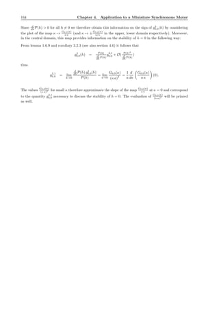
179. 4.4. Preliminary Remarks on Numerical Evaluation 165
4.4.3 How to Determine Resonances
Let us first note that by consequence of (4.36), (4.38), (4.43) and (4.45) the maps g2
k,n vanish if |n| ∈ {0, 2}.
Thus the set R of resonant frequencies as defined in GA 2.2 is given by
R = q ∈ Q | q ∈ [Ω(Jr), Ω(0)], ∃k ∈ Z : q = −2
k
= q ∈ Q q ∈
a
2
2π
4 K(Jr
a )
,
a
2
, ∃k ∈ N∗
: q = 2
k
Hence by solving the equations Ω(κ, a) = a
2
2π
4 K(κ) = 2
k with respect to κ we obtain a family
{(km, κkm ) | m = 1..M} of solutions such that the resonances h ∈ H appearing here are given by κ(hm) =
κkm .
As the Fourier coefficients g2
k,n are of size O(1/k3
) (cf. remark 1.6.10) we determine the resonances for
|k| ≤ kmax only. The value kmax ∈ N∗
is chosen in a way such that the corresponding values 2 g2
k,n(κkm )
are smaller than g2
0,0(κkm ), hence passage through resonance takes place for all the resonances with indices
k ≥ kmax (cf. section 2.3.4).
DetectResonances := proc(kmax,kappa1,kappa2)
local Resonances,Res,k,kappa,j;
global Omega,apar;
j := 0;
Resonances := array(1 .. kmax);
printf(‘******************* Detection of Resonances ***********************‘);
lprint();
for k to kmax do
Res := fsolve(Omega(kappa,apar) = 2/k,kappa,kappa1 .. kappa2);
if type(Res,float) then
j := j+1;
Resonances[j] := [k,Res];
printf(‘2 : %g-Resonance in %g......‘,k,Res);
lprint()
fi
od;
printf(‘******************* DETECTION COMPLETE ***********************‘);
lprint();
[j,table([seq(k = Resonances[k],k = 1 .. j)])]
end
In figure 4.17 a plot of the map Ω over κ and a is shown. The level curves Ω = 2
k found via the procedure
”DetectResonances” are depicted in figure 4.18 : The curves for Ω = 2 : 1, Ω = 2 : 2 and Ω = 2 : 3 (most
right to left) are clearly visible, while the curves for larger k approache the level curve Ω = 0 (i.e. a = 0).

180. 166 Chapter 4. Application to a Miniature Synchronous Motor
0
1
2
3
4
5
abar
0
0.2
0.4
0.6
0.8
1
kappa
0
0.5
1
1.5
2
2.5
omega(abar, kappa)
Figure 4.17: 3D–Graph of Ω(κ, a)
0
0.2
0.4
0.6
0.8
1
kappa
0 1 2 3 4 5
abar
Figure 4.18: Results of procedure ”DetectResonances”
Remark 4.4.1 The results of the procedure ”DetectResonances” correspond to the level curves of the
three dimensional plot of Ω(κ, a). Taking into account that Ω(0, a) = a
2 is the maximal value of Ω we see
that there exist basically three cases:
4.58 a. 0 < a < 1 The values of Ω are bounded by 2 : 4. Hence all the resonances appearing are higher order
resonances 2 : 5, 2 : 6, . . . . In view of the bounds given in lemma 1.6.10 we expect assumption
(2.33) of remark 2.3.4 to be satisfied. Hence for these values of a passage through resonance is
probable.
4.58 b. 1 < a ≤≈ 5 This is the most difficult range for the qualitative discussion. The resonances κ(hm)
corresponding to the critical frequencies 2 : 1, 2 : 2 and 2 : 3 are situated in the interior of the

181. 4.4. Preliminary Remarks on Numerical Evaluation 167
interval (0, 1), i.e. 0 < κ(hm) < Jr
a < 1. Since the maps g2
−k,−2 for k = 1, 2, 3, . . . may well be of
the same size as g2
0,0, it generally will not be possible to establish passage through resonance for all
solutions.
4.58 c. ≈ 5 ≤ a For these values of a, all resonances are ”very close” to κ = 1 (cf. figure 4.19 where a
graph of Ω together with the resonant values κkm are plotted for a = 1.1, 2.1, 4.1, 8.1). On a large
domain of the phase space it generally suffices to discuss the ”drift” in the outer zones given by
g2
0,0.
2:1
2:4
2:3
2:2
κ
Ω(κ)
✗ ✗
1
2:8
✗ ✗ ✗ ✗✗
Figure 4.19: Graph of Ω(κ) for various choices of a
4.4.4 On the Capture in Resonance
Recalling the results found in section 2.3.4 we note that it is possible that some solutions of the reduced
system (2.1) are captured near a resonance hm, i.e. satisfy |h(t) − hm| ≤ b0 |ε| for all t ≥ t0 (for some
constants b0, t0, see also (2.28)). By consequence of definition 1.5.1 the set h = hm in the (ϕ, h)–space
corresponds to the trajectory of the solution (q, p)(t; 0, P(hm)) of the Hamiltonian system (1.2) with
initial value (0, P(hm)) and thus to the level curve Lhm of H through (0, P(hm)) in the (Q, P)–space.
As the transformations (1.15), (1.86) from (q, p)–coordinates into (Q, P)–coordinates are near–identical
(up to O(ε2
)–terms), we conclude that in the case of a capture near the resonance h = hm the corre-
sponding solution (q, p)(t) satisfies
dist (Lhm , (q, p)(t)) = O(ε), ∀ t ≥ t0.
For large values of |P(hm)|, i.e. in the far upper or lower domain, the level curves Lhm are close to the
lines p = P(hm). In view of (4.1.3) a captured solution then is of the form
ϑ(τ(t)) = (P(hm) + 1) t + ε α(t, ε)
where α is bounded. If (ϕ, h)(t) is attracted by a λ 2π–periodic solution near h = hm (λ ∈ R∗
+), then the
map α approaches a λ 2π–periodic function as t → ∞.
We finally note that the values P(hm) are obtained from the values κ(hm) = κkm via the identities
P(hm) =



a/κkm in the upper domain
a κkm in the central domain
−a/κkm in the lower domain.

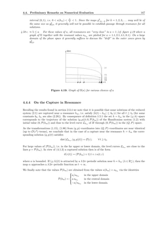
182. 168 Chapter 4. Application to a Miniature Synchronous Motor
4.4.5 Finite Convolution via Discrete Fourier Transformation
We refer the reader to [16], pages 111 ff.
calcM := proc(m) 2^(m-2)-1 end
My2Maple := proc(alpha)
local Re_a,Im_a,k;
global M;
Re_a := table([seq(k=evalc(Re(alpha[k-M])),k = 0 .. 2*M),seq(k = 0,k = 2*M+1 .. 4*M+3)]);
Im_a := table([seq(k=evalc(Im(alpha[k-M])),k = 0 .. 2*M),seq(k = 0,k = 2*M+1 .. 4*M+3)]);
[array([seq(Re_a[k],k = 0 .. 4*M+3)]),array([seq(Im_a[k],k = 0 .. 4*M+3)])]
end
LinConv := proc(Re_a, Im_a, Re_b, Im_b)
local k, DFT_a, DFT_b, Re_DFT_a, Im_DFT_a, Re_DFT_b, Im_DFT_b,
Re_ab, Im_ab;
global M, mm;
Re_DFT_a := copy(Re_a);
Im_DFT_a := copy(Im_a);
Re_DFT_b := copy(Re_b);
Im_DFT_b := copy(Im_b);
evalhf(FFT(mm, var(Re_DFT_a), var(Im_DFT_a)));
evalhf(FFT(mm, var(Re_DFT_b), var(Im_DFT_b)));
Re_ab := array([seq( Re_DFT_a[k]*Re_DFT_b[k] - Im_DFT_a[k]*Im_DFT_b[k],k=1 .. 4*M + 4)]);
Im_ab := array([seq( Re_DFT_a[k]*Im_DFT_b[k] + Im_DFT_a[k]*Re_DFT_b[k],k=1 .. 4*M + 4)]);
evalhf(iFFT(mm, var(Re_ab), var(Im_ab)));
[array([seq(Re_ab[k], k = 1 .. 4*M + 4)]), array([seq(Im_ab[k], k = 1 .. 4*M + 4)])]
end
shift2M := proc(Re_a,Im_a)
local k;
global M,cutoff;
for k from -M to M do
if abs(Re_a[2*M+k+1]) < cutoff then Re_a[2*M+k+1] := 0 fi;
if abs(Im_a[2*M+k+1]) < cutoff then Im_a[2*M+k+1] := 0 fi
od;
table([seq(k = Re_a[2*M+k+1]+I*Im_a[2*M+k+1],k = -M .. M)])
end
ComplexFold := proc(alpha1,alpha2)
local k,a,b,ab;
a := My2Maple(alpha1);
b := My2Maple(alpha2);
ab := LinConv(a[1],a[2],b[1],b[2]);
ab := shift2M(ab[1],ab[2])
end

183. 4.4. Preliminary Remarks on Numerical Evaluation 169
4.4.6 Additional Programmcode
For the interested reader we provide here the remaining code which was used to generate the output
presented in section 4.5.
MakeG00datas := proc(mm, grid, kappa1, kappa2)
local i, kappa, G00, G00val, dn, iksn, cn, u, a, b, alpha,
alphacc, beta, betacc, alphabeta, alphabetacc, abeta, bbeta,
abetacc, bbetacc, S, starti, endi;
global apar, zeta, z, rho, m, M, v, vb;
G00 := array(0 .. grid);
printf(‘******************* Calculation of G_0,0(kappa) ***********************n‘);
printf(‘--> parameter a=%g rho=%g m=%gn‘, apar, rho, m);
printf(‘--> kappa in [%g, %g]n‘, kappa1, kappa2);
printf(‘--> kappa-steps = %g n‘, (kappa2 - kappa1)/grid);
printf(‘(4*M is the size of arrays used during Discrete Fourier Transformation)n‘);
printf(‘--------------------------------------------------------------------------n‘);
printf(‘| M | kappa | G_0,0(kappa)/(a*kappa) | G_0,0(kappa)/(a*kappa)^2 |‘);
print();
M := calcM(mm);
if kappa1 = 0 then starti := 1 else starti := 0 fi;
if kappa2 = 1 then endi := grid - 1 else endi := grid fi;
for i from starti to endi do
kappa := kappa1 + i*(kappa2 - kappa1)/grid;
dn := dn_build(kappa);
iksn := iksn_build(kappa);
cn := cn_build(kappa);
a := a_build(dn, iksn);
b := b_build(kappa, cn);
alpha := alpha_build(a);
beta := beta_build(iksn, dn, b);
alphabeta := alphabeta_build(alpha, beta);
abeta := abeta_build(a, beta);
bbeta := bbeta_build(b, beta);
alphacc := alphacc_build(alpha);
alphabetacc := alphabetacc_build(alphabeta);
abetacc := abetacc_build(abeta);
bbetacc := bbetacc_build(bbeta);
S := S1_build(kappa, alpha, alphacc);
G00val := evalG00(beta,alphabeta,abeta,bbeta,alphabetacc,abetacc,bbetacc,zeta,z,S);
G00[i] := [kappa, G00val/(apar*kappa)];
printf(‘| %2.0f | %1.10f | %+1.10f | %+1.10f |‘,
M, kappa, G00val/(apar*kappa), G00val/(apar^2*kappa^2));
print()
od;
printf(‘******************** CALCULATION COMPLETE ******************n‘);
[seq(G00[i], i = starti .. endi)]
end

184. 170 Chapter 4. Application to a Miniature Synchronous Motor
MakeGk2datas := proc(k, mm, grid, kappa1, kappa2, Resh)
local i, starti, endi, kappa, Gk2, Gk2val, G00val, bbeta, bbetacc,
dn, iksn, cn, a, b, alpha, alphacc, beta, alphabeta, alphabetacc,
abeta, abetacc, S, passStr, mmm;
global apar, zeta, z, M, v, vb;
Gk2 := array(0 .. grid);
lprint();
printf(‘n**************** Calculation of 2*|G_{-k,2}(kappa)| *****************‘);
lprint();
printf(‘--> parameter a=%g rho=%g m=%gn‘, apar, rho, m);
printf(‘--> 2 : %g Resonance in %g n‘, k, Resh);
printf(‘--> kappa in [%g, %g]n‘, kappa1, kappa2);
printf(‘--> kappa-steps = %g‘, (kappa2 - kappa1)/grid);
lprint();
printf(‘(4*M is the size of arrays used during Discrete Fourier Transformation)n‘);
printf(‘-----------------------------------------------------------------------n‘);
printf(‘| M | kappa | G_%g,2(kappa)/(a*kappa) | G_0,0(kappa)/(a*kappa)
| passage |‘, -k);
print();
if kappa1 = 0 then starti := 1 else starti := 0 fi;
if kappa2 = 1 then endi := grid - 1 else endi := grid fi;
for i from starti to endi do
kappa := kappa1 + i*(kappa2 - kappa1)/grid;
M := calcM(mm);
mmm := mm;
while evalb(M < abs(k)) do
mmm := mmm + 1; M := calcM(mmm)
od;
dn := dn_build(kappa);
iksn := iksn_build(kappa);
cn := cn_build(kappa);
a := a_build(dn, iksn);
b := b_build(kappa, cn);
alpha := alpha_build(a);
beta := beta_build(iksn, dn, b);
alphabeta := alphabeta_build(alpha, beta);
abeta := abeta_build(a, beta);
bbeta := bbeta_build(b, beta);
alphacc := alphacc_build(alpha);
alphabetacc := alphabetacc_build(alphabeta);
abetacc := abetacc_build(abeta);
bbetacc := bbetacc_build(bbeta);
S := S1_build(kappa, alpha, alphacc);
Gk2val := evalGk2(k, beta, alphabeta, abeta, alphabetacc, abetacc, zeta, z, S);
Gk2[i] := [kappa, Gk2val/(apar*kappa)];
G00val := evalG00(beta,alphabeta,abeta,bbeta,alphabetacc,abetacc,bbetacc,zeta,z,S);
if abs(G00val) > Gk2val then passStr := ‘ certain ‘
else passStr := ‘ mostly ‘
fi;
printf(‘| %2.0f | %1.10f | %+1.10f | %+1.10f |%s|‘,
M, kappa, Gk2val/(apar*kappa), G00val/(apar*kappa), passStr);
print()
od;
printf(‘******************** CALCULATION COMPLETE *************************n‘);
[seq(Gk2[i], i = starti .. endi)]
end

185. 4.4. Preliminary Remarks on Numerical Evaluation 171
RunIt := proc(kappa1, kappa2, grid, Resgrid, mm, delta, CalculateResonances)
local ResonanceList, k, j, G00Plot, G00Plotdata, Gk2Plot,
Gk2Plotdata, Plot00Title, ommin, kmin, kmax, Plotk2Title,
Filek2Name, kap1, kap2, ResNr, Resh, Output;
global apar, rho, m, M, zeta, z;
M := calcM(mm);
Plot00Title := cat(‘G_0,0(kappa) ( abar=‘,convert(apar, name), ‘ , rho=‘,
convert(evalf(rho, 3), name), ‘ , m=‘, convert(m, name),‘ , M=‘,
convert(calcM(mm), name), ‘)‘);
G00Plotdata := MakeG00datas(mm, grid, kappa1, kappa2);
G00Plot := [Plot00Title, G00Plotdata];
if evalb(CalculateResonances) then
ommin := Omega(kappa2, apar);
kmin := trunc(6/ommin) + 1;
kmax := min(kmin, 10);
ResonanceList := DetectResonances(kmax, kappa1, kappa2);
if 0 < ResonanceList[1] then
Gk2Plot := array(1 .. ResonanceList[1]);
Gk2Plotdata := array(1 .. ResonanceList[1]);
for k to ResonanceList[1] do
ResNr := abs(ResonanceList[2][k][1]);
Resh := abs(ResonanceList[2][k][2]);
kap1 := Resh - delta;
kap2 := Resh + delta;
if kap1 < 0 then kap1 := Resh fi;
if 1 < kap2 then kap2 := Resh fi;
Gk2Plotdata[k] := MakeGk2datas(ResNr, mm, Resgrid, kap1, kap2, Resh);
Plotk2Title := cat(‘G_-‘, convert(ResNr, name), ‘,
2(kappa) ( abar=‘,
convert(apar, name), ‘ , rho=‘, convert(evalf(rho, 3), name), ‘m=‘,
convert(m, name), ‘M=‘, convert(calcM(mm), name), ‘)‘);
Gk2Plot[k] := [Plotk2Title, Gk2Plotdata[k]]
od
fi
else ResonanceList := [0]
fi;
[ResonanceList[1] + 2, G00Plot, seq(Gk2Plot[j], j = 1 .. ResonanceList[1])]
end

186. 172 Chapter 4. Application to a Miniature Synchronous Motor
4.5 Numerical Evaluations, Discussion Following Chapter 2
In this section we present the results found via numerical evaluation of the formulae defining the maps
G0,0 and G−k,−2 given by (4.57) together with (4.46), (4.47) in section 4.3.5. The calculations were
carried out for choices of a ∈ {0.54, 4.1, 20.38}, ̺, m ∈ {0, 1}. Each subsection to follow corresponds to a
particular set of parameters. The output of the evaluations is organized as follows:
• Graphs of
G0,0(κ)
a/κ on the upper,
G0,0(κ)
a κ on the central and
G0,0(κ)
−a/κ on the lower domains.
Recall that as κ → 1 points approach a small ε–independent neighbourhood of the seperatrix. In
the central domain (where P(h) = a κ(h)) points near the periodic solution correspond to κ → 0
while for the upper (P(h) = a/κ(h)) and lower (P(h) = −a/κ(h)) domain points tend towards ±∞
as κ → 0.
• Alphanumerical output of the calculation routines. For each of the upper, central and the
lower domain the output of the calculation scheme is given. It is divided into three parts:
– Calculation of G0,0(κ) : The output includes a header showing further specification of the
parameters followed by a listing of the values
G0,0(κ)
a κ , ±
G0,0(κ)
a/κ and
G0,0(κ)
(a κ)2 ,
G0,0(κ)
(a/κ)2 eval-
uated at 25 equidistant points in the interval [0, 1).
By looking at the values found for
G0,0(κ)
(a κ)2 near κ = 0 in the central domain, an approximation
for the value g2,1
0,0 is found (cf. section 4.4.2). The reader is invited to compare these results to
the graph depicted in figure 4.36.
– Detection of resonances: The output of the routine detecting resonances contains the list of
the ratio of the resonances found together with the corresponding value κ(hm). The maximum
order ′′
kmax′′
of resonances to be considered is set to 2 : 10 here. If no resonances were found
on the domain considered for κ the output consist of a header row and a footer row only.
– Calculation(s) of G−k,−2 : For each resonance listed the values
G−k,−2(κ)
a κ , ±
G−k,−2(κ)
a/κ are
evaluated and compared with
G0,0(κ)
a κ , ±
G0,0(κ)
a/κ . In view of the discussion in section 4.4.2
this makes it possible to decide whether a passage through the resonance is certain for all
solutions or for most solutions (i.e. up to a set of size O(ε), cf. section 2.3.4). This is indicated
in the last column with the marks certain or mostly.
• Schematic Phase Portrait A schematic sketch of the phase portrait of the reduced system
showing the average drifts (arrows) and attracting sets (light grey, if existing) closes each subsection.
Moreover resonance curves a shown (dashed) if the passage through resonance may be established
for most solutions, i.e. up to a set of order O(ε).

187. 4.5. Numerical Evaluations, Discussion Following Chapter 2 173
4.5.1 a = 0.54, ̺ = 0, m = 0
-0.7
-0.6
-0.5
-0.4
-0.3
-0.2
-0.1
0.2 0.4 0.6 0.8 1
G_0,0(kappa) ( abar=.54 , rho=0 , m=0 , M=63)
-0.16
-0.14
-0.12
-0.1
-0.08
-0.06
-0.04
-0.02
0.2 0.4 0.6 0.8 1
G_0,0(kappa) ( abar=.54 , rho=0 , m=0 , M=63)
0
0.2
0.4
0.6
0.8
0.2 0.4 0.6 0.8 1
G_0,0(kappa) ( abar=.54 , rho=0 , m=0 , M=63)
Figure 4.20: a = 0.54, ̺ = 0, m = 0 : plot of
G0,0(κ)
a/κ on the upper,
G0,0(κ)
a κ on the central and
G0,0(κ)
−a/κ
on the lower domains

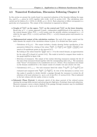
188. 174 Chapter 4. Application to a Miniature Synchronous Motor
upper domain :
*********************** Calculation of G_0,0(kappa) ***************************
--> parameter a=.54 rho=0 m=0
--> kappa in [0, .99]
--> kappa-steps = .0396
(4*M is the size of arrays used during Discrete Fourier Transformation)
---------------------------------------------------------------------------------
| M | kappa | G_0,0(kappa)/(a/kappa) | G_0,0(kappa)/(a/kappa)^2 |
| 63 | .0396000000 | -.0686447851 | -0.0050339509 |
| 63 | .0792000000 | -.1300828309 | -0.0190788152 |
| 63 | .1188000000 | -.1866895908 | -0.0410717099 |
| 63 | .1584000000 | -.2400945790 | -0.0704277431 |
| 63 | .1980000000 | -.2914430218 | -0.1068624413 |
| 63 | .2376000000 | -.3415132761 | -0.1502658415 |
| 63 | .2772000000 | -.3907754230 | -0.2005980505 |
| 63 | .3168000000 | -.4394220391 | -0.2577942629 |
| 63 | .3564000000 | -.4873850566 | -0.3216741374 |
| 63 | .3960000000 | -.5343471041 | -0.3918545430 |
| 63 | .4356000000 | -.5797537987 | -0.4676680642 |
| 63 | .4752000000 | -.6228324110 | -0.5480925217 |
| 63 | .5148000000 | -.6626210395 | -0.6316987243 |
| 63 | .5544000000 | -.6980104038 | -0.7166240146 |
| 63 | .5940000000 | -.7277974411 | -0.8005771852 |
| 63 | .6336000000 | -.7507462550 | -0.8808756058 |
| 63 | .6732000000 | -.7656480610 | -0.9545079160 |
| 63 | .7128000000 | -.7713680246 | -1.0182057925 |
| 63 | .7524000000 | -.7668630276 | -1.0684958185 |
| 63 | .7920000000 | -.7511480530 | -1.1016838111 |
| 63 | .8316000000 | -.7231714910 | -1.1136840961 |
| 63 | .8712000000 | -.6815005426 | -1.0994875420 |
| 63 | .9108000000 | -.6234780025 | -1.0515995642 |
| 63 | .9504000000 | -.5421347699 | -0.9541571951 |
| 63 | .9900000000 | -.3983523535 | -0.7303126481 |
******************** CALCULATION COMPLETE *************************
******************* Detection of Resonances ***********************
2 : 1-Resonance in +.1343870049......
2 : 2-Resonance in +.2651460995......
2 : 3-Resonance in +.3888961596......
2 : 4-Resonance in +.5027329013......
******************* DETECTION COMPLETE ***********************
*********************** Calculation of G_-k,2(kappa)| ***************************
--> parameter a=.54 rho=0 m=0
--> 2 : 1 Resonance in .134387
--> kappa in [.084387, .184387]
--> kappa-steps = .05
(4*M is the size of arrays used during Discrete Fourier Transformation)
-----------------------------------------------------------------------------------------
| M | kappa | G_-1,2(kappa)/(a/kappa) | G_0,0(kappa)/(a/kappa) | passage |
| 63 | .0843870049 | +0.0000000000 | -.1377315714 | certain |
| 63 | .1343870049 | +0.0000000000 | -.2080198644 | certain |
| 63 | .1843870049 | +0.0000000000 | -.2739679876 | certain |
******************************* CALCULATION COMPLETE **********************************

189. 4.5. Numerical Evaluations, Discussion Following Chapter 2 175
*********************** Calculation of G_-k,2(kappa)| ***************************
--> parameter a=.54 rho=0 m=0
--> 2 : 2 Resonance in .265146
--> kappa in [.215146, .315146]
--> kappa-steps = .05
(4*M is the size of arrays used during Discrete Fourier Transformation)
-----------------------------------------------------------------------------------------
| M | kappa | G_-2,2(kappa)/(a/kappa) | G_0,0(kappa)/(a/kappa) | passage |
| 63 | .2151460995 | +.4645644541 | -.3132452504 | mostly |
| 63 | .2651460995 | +.4819943004 | -.3758492763 | mostly |
| 63 | .3151460995 | +.4966052351 | -.4374026487 | mostly |
******************************* CALCULATION COMPLETE **********************************
*********************** Calculation of G_-k,2(kappa)| ***************************
--> parameter a=.54 rho=0 m=0
--> 2 : 3 Resonance in .388896
--> kappa in [.338896, .438896]
--> kappa-steps = .05
(4*M is the size of arrays used during Discrete Fourier Transformation)
-----------------------------------------------------------------------------------------
| M | kappa | G_-3,2(kappa)/(a/kappa) | G_0,0(kappa)/(a/kappa) | passage |
| 63 | .3388961596 | +0.0000000000 | -.4662836238 | certain |
| 63 | .3888961596 | +0.0000000000 | -.5260180190 | certain |
| 63 | .4388961596 | +0.0000000000 | -.5834404315 | certain |
******************************* CALCULATION COMPLETE **********************************
*********************** Calculation of G_-k,2(kappa)| ***************************
--> parameter a=.54 rho=0 m=0
--> 2 : 4 Resonance in .502732
--> kappa in [.452732, .552732]
--> kappa-steps = .05
(4*M is the size of arrays used during Discrete Fourier Transformation)
-----------------------------------------------------------------------------------------
| M | kappa | G_-4,2(kappa)/(a/kappa) | G_0,0(kappa)/(a/kappa) | passage |
| 63 | .4527329013 | +.2001595457 | -.5987298864 | certain |
| 63 | .5027329013 | +.2280917206 | -.6509090303 | certain |
| 63 | .5527329013 | +.2544413511 | -.6966249001 | certain |
******************************* CALCULATION COMPLETE **********************************
As seen in the plot on top of figure 4.20 the drift G0,0(κ) is negative for all values κ ∈ (0, 0.99] evaluated
numerically. Hence away from resonances (i.e. in the outer zone) the solutions of the corresponding
reduced system tend towards h = −∞ i.e. κ → 1 thus towards an ε–independant small neighbourhood
of the upper separatrix.
The alphanumerical output indicates that up to an O(ε)–set (cf. proposition 2.3.11) all solutions pass
through the 2 : 2 resonance arising at κkm ≈ 0.26 as |G0,0(0.26)| < G−2,2(0.26). Hence for at most an
O(ε)–set of solutions a capture in this 2 : 2 resonance is possible. The value κkm ≈ 0.26 corresponds to
P(hm) = a/κkm ≈ 2 (cf. section 4.4.4).
The remaining resonances found are passed by all solutions, as it was discussed in lemma 2.3.4.

190. 176 Chapter 4. Application to a Miniature Synchronous Motor
central domain :
******************* Calculation of G_0,0(kappa) ***********************
--> parameter a=.54 rho=0 m=0
--> kappa in [0, .99]
--> kappa-steps = .0396
(4*M is the size of arrays used during Discrete Fourier Transformation)
--------------------------------------------------------------------------------
| M | kappa | G_0,0(kappa)/(a*kappa) | G_0,0(kappa)/(a*kappa)^2 |
| 63 | .0396000000 | -.0101616353 | -.4751980619 |
| 63 | .0792000000 | -.0202893535 | -.4744050119 |
| 63 | .1188000000 | -.0303493075 | -.4730843549 |
| 63 | .1584000000 | -.0403077848 | -.4712376638 |
| 63 | .1980000000 | -.0501312599 | -.4688670030 |
| 63 | .2376000000 | -.0597864278 | -.4659747772 |
| 63 | .2772000000 | -.0692402077 | -.4625635173 |
| 63 | .3168000000 | -.0784597068 | -.4586355855 |
| 63 | .3564000000 | -.0874121242 | -.4541927725 |
| 63 | .3960000000 | -.0960645724 | -.4492357485 |
| 63 | .4356000000 | -.1043837815 | -.4437633130 |
| 63 | .4752000000 | -.1123356327 | -.4377713583 |
| 63 | .5148000000 | -.1198844445 | -.4312514191 |
| 63 | .5544000000 | -.1269918882 | -.4241886064 |
| 63 | .5940000000 | -.1336153361 | -.4165585988 |
| 63 | .6336000000 | -.1397053106 | -.4083231349 |
| 63 | .6732000000 | -.1452014534 | -.3994230249 |
| 63 | .7128000000 | -.1500259297 | -.3897668292 |
| 63 | .7524000000 | -.1540721083 | -.3792114821 |
| 63 | .7920000000 | -.1571838147 | -.3675266900 |
| 63 | .8316000000 | -.1591137393 | -.3543230793 |
| 63 | .8712000000 | -.1594287613 | -.3388871062 |
| 63 | .9108000000 | -.1572490262 | -.3197210150 |
| 63 | .9504000000 | -.1502475728 | -.2927569928 |
| 63 | .9900000000 | -.1254297127 | -.2346234806 |
******************** CALCULATION COMPLETE *************************
******************* Detection of Resonances ***********************
2 : 8-Resonance in +.5191173717......
2 : 9-Resonance in +.7483112555......
2 : 10-Resonance in +.8538470933......
******************* DETECTION COMPLETE ***********************
******************* Calculation of G_-k,2(kappa)| ***********************
--> parameter a=.54 rho=0 m=0
--> 2 : 8 Resonance in .519117
--> kappa in [.469117, .569117]
--> kappa-steps = .05
(4*M is the size of arrays used during Discrete Fourier Transformation)
-----------------------------------------------------------------------------------------
| M | kappa | G_-8,2(kappa)/(a*kappa) | G_0,0(kappa)/(a*kappa) | passage |
| 63 | .4691173717 | +.0000757834 | -.1111394979 | certain |
| 63 | .5191173717 | +.0001628013 | -.1206814887 | certain |
| 63 | .5691173717 | +.0003304881 | -.1295124702 | certain |
******************** CALCULATION COMPLETE *************************

191. 4.5. Numerical Evaluations, Discussion Following Chapter 2 177
******************* Calculation of G_-k,2(kappa)| ***********************
--> parameter a=.54 rho=0 m=0
--> 2 : 9 Resonance in .748311
--> kappa in [.698311, .798311]
--> kappa-steps = .05
(4*M is the size of arrays used during Discrete Fourier Transformation)
-----------------------------------------------------------------------------------------
| M | kappa | G_-9,2(kappa)/(a*kappa) | G_0,0(kappa)/(a*kappa) | passage |
| 63 | .6983112555 | +.0005194597 | -.1483446195 | certain |
| 63 | .7483112555 | +.0010457119 | -.1536943953 | certain |
| 63 | .7983112555 | +.0020912121 | -.1575788339 | certain |
******************** CALCULATION COMPLETE *************************
******************* Calculation of G_-k,2(kappa)| ***********************
--> parameter a=.54 rho=0 m=0
--> 2 : 10 Resonance in .853847
--> kappa in [.803847, .903847]
--> kappa-steps = .05
(4*M is the size of arrays used during Discrete Fourier Transformation)
-----------------------------------------------------------------------------------------
| M | kappa | G_-10,2(kappa)/(a*kappa) | G_0,0(kappa)/(a*kappa) | passage |
| 63 | .8038470933 | +.0008016925 | -.1578998734 | certain |
| 63 | .8538470933 | +.0018221840 | -.1595301896 | certain |
| 63 | .9038470933 | +.0043835408 | -.1578798979 | certain |
******************** CALCULATION COMPLETE *************************
As the drift G0,0(κ) is negative for all values κ ∈ (0, 0.99], ˙h in the averaged reduced system is negative
(for h > 0). Hence the solutions tend towards the invariant set κ = 0, h = 0, respectively i.e. the periodic
solution at the origin. The solutions may not be captured in the resonances arising. Together with the
results found in section 4.6 to follow, we will see that the periodic solution h = 0 is globally attractive
and stable in the entire central domain. From the last column showing
G0,0(κ)
(κ a)2 we estimate g2,1
0,0 ≈ −0.47
which coincides with the value presented in figure 4.36.

192. 178 Chapter 4. Application to a Miniature Synchronous Motor
lower domain :
************************** Calculation of G_0,0(kappa) ***************************
--> parameter a=.54 rho=0 m=0
--> kappa in [0, .99]
--> kappa-steps = .0396
(4*M is the size of arrays used during Discrete Fourier Transformation)
----------------------------------------------------------------------------------
| M | kappa | G_0,0(kappa)/(-a/kappa) | G_0,0(kappa)/(-a/kappa)^2 |
| 63 | .0396000000 | +.0796445290 | -.0058405987 |
| 63 | .0792000000 | +.1774760156 | -.0260298156 |
| 63 | .1188000000 | +.3105204651 | -.0683145023 |
| 63 | .1584000000 | +.5257107500 | -.1542084866 |
| 63 | .1980000000 | +.8767114389 | -.3214608609 |
| 63 | .2376000000 | +.7773337592 | -.3420268540 |
| 63 | .2772000000 | +.4115375150 | -.2112559244 |
| 63 | .3168000000 | +.2727148538 | -.1599927142 |
| 63 | .3564000000 | +.1994313322 | -.1316246793 |
| 63 | .3960000000 | +.1390129921 | -.1019428609 |
| 63 | .4356000000 | +.0832007341 | -.0671152589 |
| 63 | .4752000000 | +.0325510962 | -.0286449646 |
| 63 | .5148000000 | -.0113934889 | +.0108617928 |
| 63 | .5544000000 | -.0481280794 | +.0494114948 |
| 63 | .5940000000 | -.0781084755 | +.0859193230 |
| 63 | .6336000000 | -.1021867688 | +.1198991421 |
| 63 | .6732000000 | -.1212749731 | +.1511894665 |
| 63 | .7128000000 | -.1361830077 | +.1797615702 |
| 63 | .7524000000 | -.1475541227 | +.2055920776 |
| 63 | .7920000000 | -.1558358983 | +.2285593176 |
| 63 | .8316000000 | -.1612471207 | +.2483205659 |
| 63 | .8712000000 | -.1636952556 | +.2640950124 |
| 63 | .9108000000 | -.1625202959 | +.2741175659 |
| 63 | .9504000000 | -.1554663079 | +.2736207019 |
| 63 | .9900000000 | -.1291750079 | +.2368208479 |
******************** CALCULATION COMPLETE *************************
******************* Detection of Resonances ***********************
2 : 1-Resonance in +.1343870049......
2 : 2-Resonance in +.2651460995......
2 : 3-Resonance in +.3888961596......
2 : 4-Resonance in +.5027329013......
******************* DETECTION COMPLETE ***********************
******************* Calculation of G_-k,2(kappa)| ***********************
--> parameter a=.54 rho=0 m=0
--> 2 : 1 Resonance in .134387
--> kappa in [.084387, .184387]
--> kappa-steps = .05
(4*M is the size of arrays used during Discrete Fourier Transformation)
-------------------------------------------------------------------------------------------
| M | kappa | G_-1,2(kappa)/(-a/kappa) | G_0,0(kappa)/(-a/kappa) | passage |
| 63 | .0843870049 | +0.0000000000 | +.1923262653 | certain |
| 63 | .1343870049 | +0.0000000000 | +.3810181802 | certain |
| 63 | .1843870049 | +0.0000000000 | +.7503725033 | certain |
******************** CALCULATION COMPLETE *************************

193. 4.5. Numerical Evaluations, Discussion Following Chapter 2 179
******************* Calculation of G_-k,2(kappa)| ***********************
--> parameter a=.54 rho=0 m=0
--> 2 : 2 Resonance in .265146
--> kappa in [.215146, .315146]
--> kappa-steps = .05
(4*M is the size of arrays used during Discrete Fourier Transformation)
-------------------------------------------------------------------------------------------
| M | kappa | G_-2,2(kappa)/(-a/kappa) | G_0,0(kappa)/(-a/kappa) | passage |
| 63 | .2151460995 | -.0318656728 | +.9486125303 | certain |
| 63 | .2651460995 | -.0348682456 | +.4909921780 | certain |
| 63 | .3151460995 | -.0384116075 | +.2765091762 | certain |
******************** CALCULATION COMPLETE *************************
******************* Calculation of G_-k,2(kappa)| ***********************
--> parameter a=.54 rho=0 m=0
--> 2 : 3 Resonance in .388896
--> kappa in [.338896, .438896]
--> kappa-steps = .05
(4*M is the size of arrays used during Discrete Fourier Transformation)
-------------------------------------------------------------------------------------------
| M | kappa | G_-3,2(kappa)/(-a/kappa) | G_0,0(kappa)/(-a/kappa) | passage |
| 63 | .3388961596 | +0.0000000000 | +.2289045592 | certain |
| 63 | .3888961596 | +0.0000000000 | +.1494734630 | certain |
| 63 | .4388961596 | +0.0000000000 | +.0787643246 | certain |
******************** CALCULATION COMPLETE *************************
******************* Calculation of G_-k,2(kappa)| ***********************
--> parameter a=.54 rho=0 m=0
--> 2 : 4 Resonance in .502732
--> kappa in [.452732, .552732]
--> kappa-steps = .05
(4*M is the size of arrays used during Discrete Fourier Transformation)
-------------------------------------------------------------------------------------------
| M | kappa | G_-4,2(kappa)/(-a/kappa) | G_0,0(kappa)/(-a/kappa) | passage |
| 63 | .4527329013 | -.0017777368 | +.0605512470 | certain |
| 63 | .5027329013 | -.0023731029 | +.0012323718 | mostly |
| 63 | .5527329013 | -.0031129066 | -.0467229812 | certain |
******************** CALCULATION COMPLETE *************************
For κ ∈ (0, ≈ 0.5) the drift G0,0(κ)/(−a/κ) and thus ˙h is positive,
P
P=-1
Q
Figure 4.21: a = 0.54, ̺ = 0,
m = 0
while κ ∈ (≈ 0.5, 0.99) implies ˙h < 0. Thus the solutions in the
lower domain tend towards the set κ ≈ 0.5 which is equivalent to
P ≈ −a/κ ≈ −1. This attractive set contains solutions of the form
ϑ(τ(t)) ≈ ε α(t, ε) (cf. the formula found in section 4.4.4) which may
change the sign. From a physical point of view this corresponds to an
oscillation of the rotor. The 2 : 4 resonance detected in κkm ≈ 0.502
is very close to the zero of the function G0,0. As this zero and the
resonance are possibly identical, the results of section 2.3 might not
be applicable here.
For a discussion of the separatrix region (i.e. the white region in fig-
ure 4.21) we refer the reader to section 4.7.

194. 180 Chapter 4. Application to a Miniature Synchronous Motor
4.5.2 a = 0.54, ̺ = 1, m = 0
-14
-12
-10
-8
-6
-4
-2
0.2 0.4 0.6 0.8 1
G_0,0(kappa) ( abar=.54 , rho=1.0 , m=0 , M=63)
-0.35
-0.3
-0.25
-0.2
-0.15
-0.1
-0.05
0.2 0.4 0.6 0.8 1
G_0,0(kappa) ( abar=.54 , rho=1.0 , m=0 , M=63)
0
2
4
6
8
10
12
0.2 0.4 0.6 0.8 1
G_0,0(kappa) ( abar=.54 , rho=1.0 , m=0 , M=63)
Figure 4.22: a = 0.54, ̺ = 1, m = 0 : plot of
G0,0(κ)
a/κ on the upper,
G0,0(κ)
a κ on the central and
G0,0(κ)
−a/κ
on the lower domains

195. 4.5. Numerical Evaluations, Discussion Following Chapter 2 181
upper domain :
*********************** Calculation of G_0,0(kappa) ***************************
--> parameter a=.54 rho=1 m=0
--> kappa in [0, .99]
--> kappa-steps = .0396
(4*M is the size of arrays used during Discrete Fourier Transformation)
--------------------------------------------------------------------------------
| M | kappa | G_0,0(kappa)/(a/kappa) | G_0,0(kappa)/(a/kappa)^2 |
| 63 | .0396000000 | -14.1941182078 | -1.0409020019 |
| 63 | .0792000000 | -7.4260782072 | -1.0891581370 |
| 63 | .1188000000 | -5.1982391236 | -1.1436126072 |
| 63 | .1584000000 | -4.1031203872 | -1.2035819802 |
| 63 | .1980000000 | -3.4600266337 | -1.2686764323 |
| 63 | .2376000000 | -3.0424373556 | -1.3386724364 |
| 63 | .2772000000 | -2.7533895421 | -1.4134066316 |
| 63 | .3168000000 | -2.5443388122 | -1.4926787698 |
| 63 | .3564000000 | -2.3881189587 | -1.5761585127 |
| 63 | .3960000000 | -2.2681294223 | -1.6632949097 |
| 63 | .4356000000 | -2.1734264733 | -1.7532306884 |
| 63 | .4752000000 | -2.0962798153 | -1.8447262375 |
| 63 | .5148000000 | -2.0308740516 | -1.9360999292 |
| 63 | .5544000000 | -1.9725890858 | -2.0251914614 |
| 63 | .5940000000 | -1.9175930801 | -2.1093523881 |
| 63 | .6336000000 | -1.8626099345 | -2.1854623231 |
| 63 | .6732000000 | -1.8047808130 | -2.2499600802 |
| 63 | .7128000000 | -1.7415649398 | -2.2988657206 |
| 63 | .7524000000 | -1.6706337731 | -2.3277497239 |
| 63 | .7920000000 | -1.5897068156 | -2.3315699962 |
| 63 | .8316000000 | -1.4962428055 | -2.3042139205 |
| 63 | .8712000000 | -1.3867758994 | -2.2373317843 |
| 63 | .9108000000 | -1.2551877767 | -2.1170833834 |
| 63 | .9504000000 | -1.0863723838 | -1.9120153956 |
| 63 | .9900000000 | -.7994679938 | -1.4656913221 |
******************** CALCULATION COMPLETE *************************
******************* Detection of Resonances ***********************
2 : 1-Resonance in +.1343870049......
2 : 2-Resonance in +.2651460995......
2 : 3-Resonance in +.3888961596......
2 : 4-Resonance in +.5027329013......
******************* DETECTION COMPLETE ***********************
*********************** Calculation of G_-k,2(kappa)| ***************************
--> parameter a=.54 rho=1 m=0
--> 2 : 1 Resonance in .134387
--> kappa in [.084387, .184387]
--> kappa-steps = .05
(4*M is the size of arrays used during Discrete Fourier Transformation)
-----------------------------------------------------------------------------------------
| M | kappa | G_-1,2(kappa)/(a/kappa) | G_0,0(kappa)/(a/kappa) | passage |
| 63 | .0843870049 | +0.0000000000 | -7.0131241237 | certain |
| 63 | .1343870049 | +0.0000000000 | -4.6876280257 | certain |
| 63 | .1843870049 | +0.0000000000 | -3.6482952790 | certain |
******************************* CALCULATION COMPLETE **********************************

196. 182 Chapter 4. Application to a Miniature Synchronous Motor
*********************** Calculation of G_-k,2(kappa)| ***************************
--> parameter a=.54 rho=1 m=0
--> 2 : 2 Resonance in .265146
--> kappa in [.215146, .315146]
--> kappa-steps = .05
(4*M is the size of arrays used during Discrete Fourier Transformation)
-----------------------------------------------------------------------------------------
| M | kappa | G_-2,2(kappa)/(a/kappa) | G_0,0(kappa)/(a/kappa) | passage |
| 63 | .2151460995 | +.4645644541 | -3.2588621405 | certain |
| 63 | .2651460995 | +.4819943004 | -2.8312318725 | certain |
| 63 | .3151460995 | +.4966052351 | -2.5518692869 | certain |
******************************* CALCULATION COMPLETE **********************************
*********************** Calculation of G_-k,2(kappa)| ***************************
--> parameter a=.54 rho=1 m=0
--> 2 : 3 Resonance in .388896
--> kappa in [.338896, .438896]
--> kappa-steps = .05
(4*M is the size of arrays used during Discrete Fourier Transformation)
-----------------------------------------------------------------------------------------
| M | kappa | G_-3,2(kappa)/(a/kappa) | G_0,0(kappa)/(a/kappa) | passage |
| 63 | .3388961596 | +0.0000000000 | -2.4518881209 | certain |
| 63 | .3888961596 | +0.0000000000 | -2.2875287270 | certain |
| 63 | .4388961596 | +0.0000000000 | -2.1664254389 | certain |
******************************* CALCULATION COMPLETE **********************************
*********************** Calculation of G_-k,2(kappa)| ***************************
--> parameter a=.54 rho=1 m=0
--> 2 : 4 Resonance in .502732
--> kappa in [.452732, .552732]
--> kappa-steps = .05
(4*M is the size of arrays used during Discrete Fourier Transformation)
-----------------------------------------------------------------------------------------
| M | kappa | G_-4,2(kappa)/(a/kappa) | G_0,0(kappa)/(a/kappa) | passage |
| 63 | .4527329013 | +.2001595457 | -2.1382691569 | certain |
| 63 | .5027329013 | +.2280917206 | -2.0498557721 | certain |
| 63 | .5527329013 | +.2544413511 | -1.9749517859 | certain |
******************************* CALCULATION COMPLETE **********************************
central domain :
******************* Calculation of G_0,0(kappa) ***********************
--> parameter a=.54 rho=1 m=0
--> kappa in [0, .99]
--> kappa-steps = .0396
(4*M is the size of arrays used during Discrete Fourier Transformation)
--------------------------------------------------------------------------------
| M | kappa | G_0,0(kappa)/(a*kappa) | G_0,0(kappa)/(a*kappa)^2 |
| 63 | .0396000000 | -.0208515378 | -.9750999750 |
| 63 | .0792000000 | -.0416565339 | -.9740117374 |
| 63 | .1188000000 | -.0623683167 | -.9721959833 |
| 63 | .1584000000 | -.0829399403 | -.9696495088 |
| 63 | .1980000000 | -.1033240111 | -.9663674819 |
| 63 | .2376000000 | -.1234724649 | -.9623430677 |
| 63 | .2772000000 | -.1433362740 | -.9575668995 |
| 63 | .3168000000 | -.1628650526 | -.9520263552 |
| 63 | .3564000000 | -.1820065203 | -.9457045784 |
| 63 | .3960000000 | -.2007057664 | -.9385791548 |
| 63 | .4356000000 | -.2189042325 | -.9306203130 |
| 63 | .4752000000 | -.2365382917 | -.9217884546 |
| 63 | .5148000000 | -.2535372413 | -.9120307106 |
| 63 | .5544000000 | -.2698204188 | -.9012760503 |
| 63 | .5940000000 | -.2852929789 | -.8894281672 |

197. 4.5. Numerical Evaluations, Discussion Following Chapter 2 183
| 63 | .6336000000 | -.2998395469 | -.8763548299 |
| 63 | .6732000000 | -.3133143740 | -.8618713662 |
| 63 | .7128000000 | -.3255254323 | -.8457139094 |
| 63 | .7524000000 | -.3362073506 | -.8274936269 |
| 63 | .7920000000 | -.3449721435 | -.8066127562 |
| 63 | .8316000000 | -.3512110287 | -.7820957118 |
| 63 | .8712000000 | -.3538724650 | -.7522031447 |
| 63 | .9108000000 | -.3508556121 | -.7133647507 |
| 63 | .9504000000 | -.3367092493 | -.6560770695 |
| 63 | .9900000000 | -.2817046189 | -.5269446670 |
******************** CALCULATION COMPLETE *************************
******************* Detection of Resonances ***********************
2 : 8-Resonance in +.5191173717......
2 : 9-Resonance in +.7483112555......
2 : 10-Resonance in +.8538470933......
******************* DETECTION COMPLETE ***********************
******************* Calculation of G_-k,2(kappa)| ***********************
--> parameter a=.54 rho=1 m=0
--> 2 : 8 Resonance in .519117
--> kappa in [.469117, .569117]
--> kappa-steps = .05
(4*M is the size of arrays used during Discrete Fourier Transformation)
-----------------------------------------------------------------------------------------
| M | kappa | G_-8,2(kappa)/(a*kappa) | G_0,0(kappa)/(a*kappa) | passage |
| 63 | .4691173717 | +.0000757834 | -.2338690892 | certain |
| 63 | .5191173717 | +.0001628013 | -.2553488358 | certain |
| 63 | .5691173717 | +.0003304881 | -.2756710900 | certain |
******************** CALCULATION COMPLETE *************************
******************* Calculation of G_-k,2(kappa)| ***********************
--> parameter a=.54 rho=1 m=0
--> 2 : 9 Resonance in .748311
--> kappa in [.698311, .798311]
--> kappa-steps = .05
(4*M is the size of arrays used during Discrete Fourier Transformation)
-----------------------------------------------------------------------------------------
| M | kappa | G_-9,2(kappa)/(a*kappa) | G_0,0(kappa)/(a*kappa) | passage |
| 63 | .6983112555 | +.0005194597 | -.3212190507 | certain |
| 63 | .7483112555 | +.0010457119 | -.3351852498 | certain |
| 63 | .7983112555 | +.0020912121 | -.3461559201 | certain |
******************** CALCULATION COMPLETE *************************
******************* Calculation of G_-k,2(kappa)| ***********************
--> parameter a=.54 rho=1 m=0
--> 2 : 10 Resonance in .853847
--> kappa in [.803847, .903847]
--> kappa-steps = .05
(4*M is the size of arrays used during Discrete Fourier Transformation)
-----------------------------------------------------------------------------------------
| M | kappa | G_-10,2(kappa)/(a*kappa) | G_0,0(kappa)/(a*kappa) | passage |
| 63 | .8038470933 | +.0008016925 | -.3471396203 | certain |
| 63 | .8538470933 | +.0018221840 | -.3532445112 | certain |
| 63 | .9038470933 | +.0043835408 | -.3519559769 | certain |
******************** CALCULATION COMPLETE *************************

198. 184 Chapter 4. Application to a Miniature Synchronous Motor
lower domain :
************************** Calculation of G_0,0(kappa) ***************************
--> parameter a=.54 rho=1 m=0
--> kappa in [0, .99]
--> kappa-steps = .0396
(4*M is the size of arrays used during Discrete Fourier Transformation)
----------------------------------------------------------------------------------
| M | kappa | G_0,0(kappa)/(-a/kappa) | G_0,0(kappa)/(-a/kappa)^2 |
| 63 | .0396000000 | +13.2055101840 | -.9684040801 |
| 63 | .0792000000 | +6.4750426365 | -.9496729200 |
| 63 | .1188000000 | +4.3256140415 | -.9516350891 |
| 63 | .1584000000 | +3.3950590710 | -.9958839941 |
| 63 | .1980000000 | +3.0552187840 | -1.1202468874 |
| 63 | .2376000000 | +2.4926282995 | -1.0967564518 |
| 63 | .2772000000 | +1.7938434247 | -.9208396246 |
| 63 | .3168000000 | +1.4035556813 | -.8234193330 |
| 63 | .3564000000 | +1.1332772528 | -.7479629868 |
| 63 | .3960000000 | +.9141057892 | -.6703442454 |
| 63 | .4356000000 | +.7274598044 | -.5868175756 |
| 63 | .4752000000 | +.5670202826 | -.4989778487 |
| 63 | .5148000000 | +.4295771905 | -.4095302549 |
| 63 | .5544000000 | +.3122502478 | -.3205769211 |
| 63 | .5940000000 | +.2121129891 | -.2333242880 |
| 63 | .6336000000 | +.1264754786 | -.1483978949 |
| 63 | .6732000000 | +.0530401909 | -.0661234380 |
| 63 | .7128000000 | -.0100534027 | +.0132704915 |
| 63 | .7524000000 | -.0642396849 | +.0895072943 |
| 63 | .7920000000 | -.1105416397 | +.1621277382 |
| 63 | .8316000000 | -.1495505577 | +.2303078588 |
| 63 | .8712000000 | -.1813097835 | +.2925131175 |
| 63 | .9108000000 | -.2049101475 | +.3456151155 |
| 63 | .9504000000 | -.2168489325 | +.3816541212 |
| 63 | .9900000000 | -.1960317450 | +.3593915325 |
******************** CALCULATION COMPLETE *************************
******************* Detection of Resonances ***********************
2 : 1-Resonance in +.1343870049......
2 : 2-Resonance in +.2651460995......
2 : 3-Resonance in +.3888961596......
2 : 4-Resonance in +.5027329013......
******************* DETECTION COMPLETE ***********************
******************* Calculation of G_-k,2(kappa)| ***********************
--> parameter a=.54 rho=1 m=0
--> 2 : 1 Resonance in .134387
--> kappa in [.084387, .184387]
--> kappa-steps = .05
(4*M is the size of arrays used during Discrete Fourier Transformation)
-------------------------------------------------------------------------------------------
| M | kappa | G_-1,2(kappa)/(-a/kappa) | G_0,0(kappa)/(-a/kappa) | passage |
| 63 | .0843870049 | +0.0000000000 | +6.0695030868 | certain |
| 63 | .1343870049 | +0.0000000000 | +3.8651670456 | certain |
| 63 | .1843870049 | +0.0000000000 | +3.1332914693 | certain |
******************** CALCULATION COMPLETE *************************

199. 4.5. Numerical Evaluations, Discussion Following Chapter 2 185
******************* Calculation of G_-k,2(kappa)| ***********************
--> parameter a=.54 rho=1 m=0
--> 2 : 2 Resonance in .265146
--> kappa in [.215146, .315146]
--> kappa-steps = .05
(4*M is the size of arrays used during Discrete Fourier Transformation)
-------------------------------------------------------------------------------------------
| M | kappa | G_-2,2(kappa)/(-a/kappa) | G_0,0(kappa)/(-a/kappa) | passage |
| 63 | .2151460995 | -.0318656728 | +2.9059731667 | certain |
| 63 | .2651460995 | -.0348682456 | +1.9643521831 | certain |
| 63 | .3151460995 | -.0384116075 | +1.4166207960 | certain |
******************** CALCULATION COMPLETE *************************
******************* Calculation of G_-k,2(kappa)| ***********************
--> parameter a=.54 rho=1 m=0
--> 2 : 3 Resonance in .388896
--> kappa in [.338896, .438896]
--> kappa-steps = .05
(4*M is the size of arrays used during Discrete Fourier Transformation)
---------------------------------------------------------------------------------_----------
| M | kappa | G_-3,2(kappa)/(-a/kappa) | G_0,0(kappa)/(-a/kappa) | passage |
| 63 | .3388961596 | +0.0000000000 | +1.2443227670 | certain |
| 63 | .3888961596 | +0.0000000000 | +.9507467398 | certain |
| 63 | .4388961596 | +0.0000000000 | +.7131588392 | certain |
******************** CALCULATION COMPLETE *************************
******************* Calculation of G_-k,2(kappa)| ***********************
--> parameter a=.54 rho=1 m=0
--> 2 : 4 Resonance in .502732
--> kappa in [.452732, .552732]
--> kappa-steps = .05
(4*M is the size of arrays used during Discrete Fourier Transformation)
-------------------------------------------------------------------------------------------
| M | kappa | G_-4,2(kappa)/(-a/kappa) | G_0,0(kappa)/(-a/kappa) | passage |
| 63 | .4527329013 | -.0017777368 | +.6550440373 | certain |
| 63 | .5027329013 | -.0023731029 | +.4691922593 | certain |
| 63 | .5527329013 | -.0031129066 | +.3168229222 | certain |
******************** CALCULATION COMPLETE *************************
The qualitative behaviour is very similar to the preceeding situation
P
P=-1
Q
Figure 4.23: a = 0.54, ̺ = 1,
m = 0
of section 4.5.1. Due to ̺ = 1 the drift remote from the separatrices,
in the upper and lower domain becomes much larger than for ̺ = 0.
As for the same reason capture in resonances (and in particular in the
2 : 2 resonance at κkm ≈ 0.26 for the upper domain) does not appear.
The attractive set in the lower domain moves to P ≈ −0.78. The
physical interpretation then is different. As ϑ(τ(t)) is of the form
0.22 t+ε α(t, ε), the rotor does not oscillate but rotate here. However,
the mean angular speed of the rotor varies around 0.22 ω (with respect
to time τ) compared to the much larger angular speed ω of the periodic
solution h = 0 (or, equivalently (Q, P) = (0, 0)). Hence for solutions
attracted in P ≈ −0.78 the synchronous motor rotates but with a
slow speed that periodically increases and decreases.

200. 186 Chapter 4. Application to a Miniature Synchronous Motor
4.5.3 a = 0.54, ̺ = 0, m = 1
-1.2
-1.1
-1
-0.9
-0.8
-0.7
-0.6
0.2 0.4 0.6 0.8 1
G_0,0(kappa) ( abar=.54 , rho=0 , m=1. , M=63)
-0.16
-0.14
-0.12
-0.1
-0.08
-0.06
-0.04
-0.02
0.2 0.4 0.6 0.8 1
G_0,0(kappa) ( abar=.54 , rho=0 , m=1. , M=63)
-0.4
-0.2
0
0.2
0.4
0.2 0.4 0.6 0.8 1
G_0,0(kappa) ( abar=.54 , rho=0 , m=1. , M=63)
Figure 4.24: a = 0.54, ̺ = 0, m = 1 : plot of
G0,0(κ)
a/κ on the upper,
G0,0(κ)
a κ on the central and
G0,0(κ)
−a/κ
on the lower domains

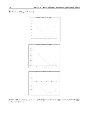
201. 4.5. Numerical Evaluations, Discussion Following Chapter 2 187
upper domain :
*********************** Calculation of G_0,0(kappa) ***************************
--> parameter a=.54 rho=0 m=1
--> kappa in [0, .99]
--> kappa-steps = .0396
(4*M is the size of arrays used during Discrete Fourier Transformation)
--------------------------------------------------------------------------------
| M | kappa | G_0,0(kappa)/(a/kappa) | G_0,0(kappa)/(a/kappa)^2 |
| 63 | .0396000000 | -.5684486690 | -.0416862357 |
| 63 | .0792000000 | -.6292972086 | -.0922969239 |
| 63 | .1188000000 | -.6849175690 | -.1506818651 |
| 63 | .1584000000 | -.7369333226 | -.2161671079 |
| 63 | .1980000000 | -.7864811552 | -.2883764235 |
| 63 | .2376000000 | -.8343280457 | -.3671043401 |
| 63 | .2772000000 | -.8809295277 | -.4522104909 |
| 63 | .3168000000 | -.9264600119 | -.5435232070 |
| 63 | .3564000000 | -.9708290474 | -.6407471713 |
| 63 | .3960000000 | -1.0136918647 | -.7433740341 |
| 63 | .4356000000 | -1.0544606008 | -.8505982180 |
| 63 | .4752000000 | -1.0923215199 | -.9612429375 |
| 63 | .5148000000 | -1.1262622058 | -1.0737033029 |
| 63 | .5544000000 | -1.1551105812 | -1.1859135300 |
| 63 | .5940000000 | -1.1775845283 | -1.2953429811 |
| 63 | .6336000000 | -1.1923469710 | -1.3990204459 |
| 63 | .6732000000 | -1.1980568549 | -1.4935775458 |
| 63 | .7128000000 | -1.1934016797 | -1.5752902172 |
| 63 | .7524000000 | -1.1770911815 | -1.6400803796 |
| 63 | .7920000000 | -1.1477803050 | -1.6834111140 |
| 63 | .8316000000 | -1.1038588667 | -1.6999426548 |
| 63 | .8712000000 | -1.0429454849 | -1.6826187157 |
| 63 | .9108000000 | -.9605278154 | -1.6200902486 |
| 63 | .9504000000 | -.8449448892 | -1.4871030049 |
| 63 | .9900000000 | -.6323385422 | -1.1592873274 |
******************** CALCULATION COMPLETE *************************
******************* Detection of Resonances ***********************
2 : 1-Resonance in +.1343870049......
2 : 2-Resonance in +.2651460995......
2 : 3-Resonance in +.3888961596......
2 : 4-Resonance in +.5027329013......
******************* DETECTION COMPLETE ***********************
*********************** Calculation of G_-k,2(kappa)| ***************************
--> parameter a=.54 rho=0 m=1
--> 2 : 1 Resonance in .134387
--> kappa in [.084387, .184387]
--> kappa-steps = .05
(4*M is the size of arrays used during Discrete Fourier Transformation)
-----------------------------------------------------------------------------------------
| M | kappa | G_-1,2(kappa)/(a/kappa) | G_0,0(kappa)/(a/kappa) | passage |
| 63 | .0843870049 | +0.0000000000 | -.6368394368 | certain |
| 63 | .1343870049 | +0.0000000000 | -.7057495124 | certain |
| 63 | .1843870049 | +0.0000000000 | -.7696721503 | certain |
******************************* CALCULATION COMPLETE **********************************

202. 188 Chapter 4. Application to a Miniature Synchronous Motor
*********************** Calculation of G_-k,2(kappa)| ***************************
--> parameter a=.54 rho=0 m=1
--> 2 : 2 Resonance in .265146
--> kappa in [.215146, .315146]
--> kappa-steps = .05
(4*M is the size of arrays used during Discrete Fourier Transformation)
-----------------------------------------------------------------------------------------
| M | kappa | G_-2,2(kappa)/(a/kappa) | G_0,0(kappa)/(a/kappa) | passage |
| 63 | .2151460995 | +.4645644541 | -.8073733772 | certain |
| 63 | .2651460995 | +.4819943004 | -.8668605718 | certain |
| 63 | .3151460995 | +.4966052351 | -.9245801579 | certain |
******************************* CALCULATION COMPLETE **********************************
*********************** Calculation of G_-k,2(kappa)| ***************************
--> parameter a=.54 rho=0 m=1
--> 2 : 3 Resonance in .388896
--> kappa in [.338896, .438896]
--> kappa-steps = .05
(4*M is the size of arrays used during Discrete Fourier Transformation)
-----------------------------------------------------------------------------------------
| M | kappa | G_-3,2(kappa)/(a/kappa) | G_0,0(kappa)/(a/kappa) | passage |
| 63 | .3388961596 | +0.0000000000 | -.9513767685 | certain |
| 63 | .3888961596 | +0.0000000000 | -1.0061367346 | certain |
| 63 | .4388961596 | +0.0000000000 | -1.0577356779 | certain |
******************************* CALCULATION COMPLETE **********************************
*********************** Calculation of G_-k,2(kappa)| ***************************
--> parameter a=.54 rho=0 m=1
--> 2 : 4 Resonance in .502732
--> kappa in [.452732, .552732]
--> kappa-steps = .05
(4*M is the size of arrays used during Discrete Fourier Transformation)
-----------------------------------------------------------------------------------------
| M | kappa | G_-4,2(kappa)/(a/kappa) | G_0,0(kappa)/(a/kappa) | passage |
| 63 | .4527329013 | +.2001595457 | -1.0712531265 | certain |
| 63 | .5027329013 | +.2280917206 | -1.1164024575 | certain |
| 63 | .5527329013 | +.2544413511 | -1.1540153912 | certain |
******************************* CALCULATION COMPLETE **********************************
central domain :
******************* Calculation of G_0,0(kappa) ***********************
--> parameter a=.54 rho=0 m=1
--> kappa in [0, .99]
--> kappa-steps = .0396
(4*M is the size of arrays used during Discrete Fourier Transformation)
--------------------------------------------------------------------------------
| M | kappa | G_0,0(kappa)/(a*kappa) | G_0,0(kappa)/(a*kappa)^2 |
| 63 | .0396000000 | -.0101616353 | -.4751980619 |
| 63 | .0792000000 | -.0202893535 | -.4744050119 |
| 63 | .1188000000 | -.0303493075 | -.4730843549 |
| 63 | .1584000000 | -.0403077848 | -.4712376638 |
| 63 | .1980000000 | -.0501312599 | -.4688670030 |
| 63 | .2376000000 | -.0597864278 | -.4659747772 |
| 63 | .2772000000 | -.0692402077 | -.4625635173 |
| 63 | .3168000000 | -.0784597068 | -.4586355855 |
| 63 | .3564000000 | -.0874121242 | -.4541927725 |
| 63 | .3960000000 | -.0960645724 | -.4492357485 |
| 63 | .4356000000 | -.1043837815 | -.4437633130 |
| 63 | .4752000000 | -.1123356327 | -.4377713583 |
| 63 | .5148000000 | -.1198844445 | -.4312514191 |
| 63 | .5544000000 | -.1269918882 | -.4241886064 |
| 63 | .5940000000 | -.1336153361 | -.4165585988 |

203. 4.5. Numerical Evaluations, Discussion Following Chapter 2 189
| 63 | .6336000000 | -.1397053106 | -.4083231349 |
| 63 | .6732000000 | -.1452014534 | -.3994230249 |
| 63 | .7128000000 | -.1500259297 | -.3897668292 |
| 63 | .7524000000 | -.1540721083 | -.3792114821 |
| 63 | .7920000000 | -.1571838147 | -.3675266900 |
| 63 | .8316000000 | -.1591137393 | -.3543230793 |
| 63 | .8712000000 | -.1594287613 | -.3388871062 |
| 63 | .9108000000 | -.1572490262 | -.3197210150 |
| 63 | .9504000000 | -.1502475728 | -.2927569928 |
| 63 | .9900000000 | -.1254297127 | -.2346234806 |
******************** CALCULATION COMPLETE *************************
******************* Detection of Resonances ***********************
2 : 8-Resonance in +.5191173717......
2 : 9-Resonance in +.7483112555......
2 : 10-Resonance in +.8538470933......
******************* DETECTION COMPLETE ***********************
******************* Calculation of G_-k,2(kappa)| ***********************
--> parameter a=.54 rho=0 m=1
--> 2 : 8 Resonance in .519117
--> kappa in [.469117, .569117]
--> kappa-steps = .05
(4*M is the size of arrays used during Discrete Fourier Transformation)
-----------------------------------------------------------------------------------------
| M | kappa | G_-8,2(kappa)/(a*kappa) | G_0,0(kappa)/(a*kappa) | passage |
| 63 | .4691173717 | +.0000757834 | -.1111394979 | certain |
| 63 | .5191173717 | +.0001628013 | -.1206814887 | certain |
| 63 | .5691173717 | +.0003304881 | -.1295124702 | certain |
******************** CALCULATION COMPLETE *************************
******************* Calculation of G_-k,2(kappa)| ***********************
--> parameter a=.54 rho=0 m=1
--> 2 : 9 Resonance in .748311
--> kappa in [.698311, .798311]
--> kappa-steps = .05
(4*M is the size of arrays used during Discrete Fourier Transformation)
-----------------------------------------------------------------------------------------
| M | kappa | G_-9,2(kappa)/(a*kappa) | G_0,0(kappa)/(a*kappa) | passage |
| 63 | .6983112555 | +.0005194597 | -.1483446195 | certain |
| 63 | .7483112555 | +.0010457119 | -.1536943953 | certain |
| 63 | .7983112555 | +.0020912121 | -.1575788339 | certain |
******************** CALCULATION COMPLETE *************************
******************* Calculation of G_-k,2(kappa)| ***********************
--> parameter a=.54 rho=0 m=1
--> 2 : 10 Resonance in .853847
--> kappa in [.803847, .903847]
--> kappa-steps = .05
(4*M is the size of arrays used during Discrete Fourier Transformation)
-----------------------------------------------------------------------------------------
| M | kappa | G_-10,2(kappa)/(a*kappa) | G_0,0(kappa)/(a*kappa) | passage |
| 63 | .8038470933 | +.0008016925 | -.1578998734 | certain |
| 63 | .8538470933 | +.0018221840 | -.1595301896 | certain |
| 63 | .9038470933 | +.0043835408 | -.1578798979 | certain |
******************** CALCULATION COMPLETE *************************

204. 190 Chapter 4. Application to a Miniature Synchronous Motor
lower domain :
************************** Calculation of G_0,0(kappa) ***************************
--> parameter a=.54 rho=0 m=1
--> kappa in [0, .99]
--> kappa-steps = .0396
(4*M is the size of arrays used during Discrete Fourier Transformation)
----------------------------------------------------------------------------------
| M | kappa | G_0,0(kappa)/(-a/kappa) | G_0,0(kappa)/(-a/kappa)^2 |
| 63 | .0396000000 | -.4201593548 | +.0308116860 |
| 63 | .0792000000 | -.3217383621 | +.0471882931 |
| 63 | .1188000000 | -.1877075130 | +.0412956528 |
| 63 | .1584000000 | +.0288720063 | -.0084691218 |
| 63 | .1980000000 | +.3816733055 | -.1399468786 |
| 63 | .2376000000 | +.2845189896 | -.1251883554 |
| 63 | .2772000000 | -.0786165896 | +.0403565160 |
| 63 | .3168000000 | -.2143231189 | +.1257362297 |
| 63 | .3564000000 | -.2840126584 | +.1874483545 |
| 63 | .3960000000 | -.3403317684 | +.2495766301 |
| 63 | .4356000000 | -.3915060679 | +.3158148948 |
| 63 | .4752000000 | -.4369380127 | +.3845054511 |
| 63 | .5148000000 | -.4750346552 | +.4528663713 |
| 63 | .5544000000 | -.5052282567 | +.5187010103 |
| 63 | .5940000000 | -.5278955627 | +.5806851189 |
| 63 | .6336000000 | -.5437874848 | +.6380439822 |
| 63 | .6732000000 | -.5536837671 | +.6902590963 |
| 63 | .7128000000 | -.5582166628 | +.7368459949 |
| 63 | .7524000000 | -.5577822765 | +.7771766386 |
| 63 | .7920000000 | -.5524681503 | +.8102866204 |
| 63 | .8316000000 | -.5419344965 | +.8345791246 |
| 63 | .8712000000 | -.5251401980 | +.8472261861 |
| 63 | .9108000000 | -.4995701088 | +.8426082503 |
| 63 | .9504000000 | -.4582764271 | +.8065665118 |
| 63 | .9900000000 | -.3631611966 | +.6657955272 |
******************** CALCULATION COMPLETE *************************
******************* Detection of Resonances ***********************
2 : 1-Resonance in +.1343870049......
2 : 2-Resonance in +.2651460995......
2 : 3-Resonance in +.3888961596......
2 : 4-Resonance in +.5027329013......
******************* DETECTION COMPLETE ***********************
******************* Calculation of G_-k,2(kappa)| ***********************
--> parameter a=.54 rho=0 m=1
--> 2 : 1 Resonance in .134387
--> kappa in [.084387, .184387]
--> kappa-steps = .05
(4*M is the size of arrays used during Discrete Fourier Transformation)
-------------------------------------------------------------------------------------------
| M | kappa | G_-1,2(kappa)/(-a/kappa) | G_0,0(kappa)/(-a/kappa) | passage |
| 63 | .0843870049 | +0.0000000000 | -.3067816000 | certain |
| 63 | .1343870049 | +0.0000000000 | -.1167114676 | certain |
| 63 | .1843870049 | +0.0000000000 | +.2546683406 | certain |
******************** CALCULATION COMPLETE *************************

205. 4.5. Numerical Evaluations, Discussion Following Chapter 2 191
******************* Calculation of G_-k,2(kappa)| ***********************
--> parameter a=.54 rho=0 m=1
--> 2 : 2 Resonance in .265146
--> kappa in [.215146, .315146]
--> kappa-steps = .05
(4*M is the size of arrays used during Discrete Fourier Transformation)
-------------------------------------------------------------------------------------------
| M | kappa | G_-2,2(kappa)/(-a/kappa) | G_0,0(kappa)/(-a/kappa) | passage |
| 63 | .2151460995 | -.0318656728 | +.4544844035 | certain |
| 63 | .2651460995 | -.0348682456 | -.0000191174 | mostly |
| 63 | .3151460995 | -.0384116075 | -.2106683329 | certain |
******************** CALCULATION COMPLETE *************************
******************* Calculation of G_-k,2(kappa)| ***********************
--> parameter a=.54 rho=0 m=1
--> 2 : 3 Resonance in .388896
--> kappa in [.338896, .438896]
--> kappa-steps = .05
(4*M is the size of arrays used during Discrete Fourier Transformation)
-------------------------------------------------------------------------------------------
| M | kappa | G_-3,2(kappa)/(-a/kappa) | G_0,0(kappa)/(-a/kappa) | passage |
| 63 | .3388961596 | +0.0000000000 | -.2561885854 | certain |
| 63 | .3888961596 | +0.0000000000 | -.3306452525 | certain |
| 63 | .4388961596 | +0.0000000000 | -.3955309217 | certain |
******************** CALCULATION COMPLETE *************************
******************* Calculation of G_-k,2(kappa)| ***********************
--> parameter a=.54 rho=0 m=1
--> 2 : 4 Resonance in .502732
--> kappa in [.452732, .552732]
--> kappa-steps = .05
(4*M is the size of arrays used during Discrete Fourier Transformation)
-------------------------------------------------------------------------------------------
| M | kappa | G_-4,2(kappa)/(-a/kappa) | G_0,0(kappa)/(-a/kappa) | passage |
| 63 | .4527329013 | -.0017777368 | -.4119719930 | certain |
| 63 | .5027329013 | -.0023731029 | -.4642610553 | certain |
| 63 | .5527329013 | -.0031129066 | -.5041134724 | certain |
******************** CALCULATION COMPLETE *************************
The calculations carried out for the upper and central domain yield
P
P=-1
Q
Figure 4.25: a = 0.54, ̺ = 0,
m = 1
the same qualitative interpretation as in section 4.5.2. By ways of
contrast the drift in the lower domain has two zeroes. The first at
P ≈ −3.8 indicates a repulsive set while the second at P ≈ −2 cor-
responds to an attractive area. As this zero and the 2 : 2 resonance
are close and possibly identical, the results of section 2.3 might not
be applicable here. However we note that P < −1 physically corre-
sponds to negative values for d
dτ ϑ. Thus the solutions in the lower
domain are attracted by a region implying backward rotation. As we
consider the case of an external torque m = 1 this is not surprising if
the load is sufficiently large to compete with the force of the motor.

206. 192 Chapter 4. Application to a Miniature Synchronous Motor
4.5.4 a = 4.1, ̺ = 0, m = 0
-0.16
-0.14
-0.12
-0.1
-0.08
-0.06
-0.04
-0.02
0.2 0.4 0.6 0.8 1
G_0,0(kappa) ( abar=4.1 , rho=0 , m=0 , M=63)
-0.24
-0.22
-0.2
-0.18
-0.16
-0.14
-0.12
-0.1
-0.08
-0.06
-0.04
-0.02
0.2 0.4 0.6 0.8 1
G_0,0(kappa) ( abar=4.1 , rho=0 , m=0 , M=63)
0
0.1
0.2
0.3
0.4
0.5
0.2 0.4 0.6 0.8 1
G_0,0(kappa) ( abar=4.1 , rho=0 , m=0 , M=63)
Figure 4.26: a = 4.1, ̺ = 0, m = 0 : plot of
G0,0(κ)
a/κ on the upper,
G0,0(κ)
a κ on the central and
G0,0(κ)
−a/κ on
the lower domains

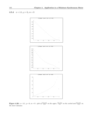
207. 4.5. Numerical Evaluations, Discussion Following Chapter 2 193
upper domain :
*********************** Calculation of G_0,0(kappa) ***************************
--> parameter a=4.1 rho=0 m=0
--> kappa in [0, .99]
--> kappa-steps = .0396
(4*M is the size of arrays used during Discrete Fourier Transformation)
--------------------------------------------------------------------------------
| M | kappa | G_0,0(kappa)/(a/kappa) | G_0,0(kappa)/(a/kappa)^2 |
| 63 | .0396000000 | -.0095669817 | -.0000924030 |
| 63 | .0792000000 | -.0189572528 | -.0003661986 |
| 63 | .1188000000 | -.0281792944 | -.0008165122 |
| 63 | .1584000000 | -.0372402044 | -.0014387435 |
| 63 | .1980000000 | -.0461457952 | -.0022285042 |
| 63 | .2376000000 | -.0549006459 | -.0031815593 |
| 63 | .2772000000 | -.0635081130 | -.0042937680 |
| 63 | .3168000000 | -.0719702944 | -.0055610217 |
| 63 | .3564000000 | -.0802879409 | -.0069791761 |
| 63 | .3960000000 | -.0884603026 | -.0085439706 |
| 63 | .4356000000 | -.0964848886 | -.0102509310 |
| 63 | .4752000000 | -.1043571107 | -.0120952436 |
| 63 | .5148000000 | -.1120697574 | -.0140715880 |
| 63 | .5544000000 | -.1196122176 | -.0161739057 |
| 63 | .5940000000 | -.1269693146 | -.0183950665 |
| 63 | .6336000000 | -.1341195160 | -.0207263720 |
| 63 | .6732000000 | -.1410320897 | -.0231567811 |
| 63 | .7128000000 | -.1476623949 | -.0256716475 |
| 63 | .7524000000 | -.1539436566 | -.0282505383 |
| 63 | .7920000000 | -.1597715731 | -.0308631916 |
| 63 | .8316000000 | -.1649727806 | -.0334613083 |
| 63 | .8712000000 | -.1692316049 | -.0359596522 |
| 63 | .9108000000 | -.1718847586 | -.0381835702 |
| 63 | .9504000000 | -.1711115173 | -.0396644844 |
| 63 | .9900000000 | -.1552516904 | -.0374876032 |
******************** CALCULATION COMPLETE *************************
******************* Detection of Resonances ***********************
2 : 1-Resonance in +.8038707404......
2 : 2-Resonance in +.9878039867......
******************* DETECTION COMPLETE ***********************
*********************** Calculation of G_-k,2(kappa)| ***************************
--> parameter a=4.1 rho=0 m=0
--> 2 : 1 Resonance in .803870
--> kappa in [.753870, .853870]
--> kappa-steps = .05
(4*M is the size of arrays used during Discrete Fourier Transformation)
-----------------------------------------------------------------------------------------
| M | kappa | G_-1,2(kappa)/(a/kappa) | G_0,0(kappa)/(a/kappa) | passage |
| 63 | .7538707404 | +0.0000000000 | -.1541690185 | certain |
| 63 | .8038707404 | +0.0000000000 | -.1614070977 | certain |
| 63 | .8538707404 | +0.0000000000 | -.1675141054 | certain |
******************************* CALCULATION COMPLETE **********************************

208. 194 Chapter 4. Application to a Miniature Synchronous Motor
*********************** Calculation of 2*|G_-k,2(kappa)| ***************************
--> parameter abar=4.1 rho=0 m=0
--> 2 : 2 Resonance in .987803
--> kappa in [.937803, .987803]
--> kappa-steps = .025
(4*M is the size of arrays used during Discrete Fourier Transformation)
-----------------------------------------------------------------------------------------
| M | kappa | G_-2,2(kappa)/(a/kappa) | G_0,0(kappa)/(a/kappa) | passage |
| 63 | .9378039867 | +1.1010778373 | -.1719643559 | mostly |
| 63 | .9628039867 | +.5373629107 | -.1692869165 | mostly |
| 63 | .9878039867 | +.3885728462 | -.1576711399 | mostly |
******************************* CALCULATION COMPLETE **********************************
We conclude that up to an O(ε)–set all orbits pass through the 2 : 2 resonance at κkm ≈ 0.988 situated
close to the upper separatrix.
central domain :
******************* Calculation of G_0,0(kappa) ***********************
--> parameter a=4.1 rho=0 m=0
--> kappa in [0, .99]
--> kappa-steps = .0396
(4*M is the size of arrays used during Discrete Fourier Transformation)
--------------------------------------------------------------------------------
| M | kappa | G_0,0(kappa)/(a*kappa) | G_0,0(kappa)/(a*kappa)^2 |
| 63 | .0396000000 | -.0183348688 | -.1129272532 |
| 63 | .0792000000 | -.0364810169 | -.1123460733 |
| 63 | .1188000000 | -.0542535008 | -.1113851950 |
| 63 | .1584000000 | -.0714749993 | -.1100563551 |
| 63 | .1980000000 | -.0879797762 | -.1083761718 |
| 63 | .2376000000 | -.1036177765 | -.1063662812 |
| 63 | .2772000000 | -.1182588207 | -.1040534445 |
| 63 | .3168000000 | -.1317968033 | -.1014695763 |
| 63 | .3564000000 | -.1441537322 | -.0986516467 |
| 63 | .3960000000 | -.1552833893 | -.0956414075 |
| 63 | .4356000000 | -.1651743492 | -.0924849096 |
| 63 | .4752000000 | -.1738521029 | -.0892318012 |
| 63 | .5148000000 | -.1813801006 | -.0859344384 |
| 63 | .5544000000 | -.1878597129 | -.0826469014 |
| 63 | .5940000000 | -.1934294449 | -.0794240966 |
| 63 | .6336000000 | -.1982643239 | -.0763212629 |
| 63 | .6732000000 | -.2025773916 | -.0733944146 |
| 63 | .7128000000 | -.2066270581 | -.0707026423 |
| 63 | .7524000000 | -.2107375600 | -.0683139352 |
| 63 | .7920000000 | -.2153464056 | -.0663175676 |
| 63 | .8316000000 | -.2211019890 | -.0648476604 |
| 63 | .8712000000 | -.2290058009 | -.0641128023 |
| 63 | .9108000000 | -.2399676172 | -.0642607456 |
| 63 | .9504000000 | -.2444025627 | -.0627213606 |
| 63 | .9900000000 | -.1776456195 | -.0437658584 |
******************** CALCULATION COMPLETE *************************
******************* Detection of Resonances ***********************
2 : 1-Resonance in +.3075848728......
2 : 2-Resonance in +.9867635460......
******************* DETECTION COMPLETE ***********************

209. 4.5. Numerical Evaluations, Discussion Following Chapter 2 195
******************* Calculation of G_-k,2(kappa)| ***********************
--> parameter a=4.1 rho=0 m=0
--> 2 : 1 Resonance in .307584
--> kappa in [.257584, .357584]
--> kappa-steps = .05
(4*M is the size of arrays used during Discrete Fourier Transformation)
-----------------------------------------------------------------------------------------
| M | kappa | G_-1,2(kappa)/(a*kappa) | G_0,0(kappa)/(a*kappa) | passage |
| 63 | .2575848728 | +.1614991274 | -.1111385236 | mostly |
| 63 | .3075848728 | +.2323316952 | -.1287495137 | mostly |
| 63 | .3575848728 | +.3173595687 | -.1445046992 | mostly |
******************** CALCULATION COMPLETE *************************
******************* Calculation of 2*|G_-k,2(kappa)| ***********************
--> parameter abar=4.1 rho=0 m=0
--> 2 : 2 Resonance in .986763
--> kappa in [.936763, .986763]
--> kappa-steps = .025
(4*M is the size of arrays used during Discrete Fourier Transformation)
-----------------------------------------------------------------------------------------
| M | kappa | G_-2,2(kappa)/(a*kappa) | G_0,0(kappa)/(a*kappa) | passage |
| 63 | .9367635460 | +.1340754295 | -.2461359773 | certain |
| 63 | .9617635460 | +.1540029415 | -.2354069917 | certain |
| 63 | .9867635460 | +.1516329740 | -.1838326901 | certain |
******************** CALCULATION COMPLETE *************************
For this choice of parameters all solutions up to a set of size O(ε) pass through the 2 : 1 resonance at
κkm ≈ 0.3 (i.e. P(hm) ≈ 1.23 of the central domain). The remaining solutions may possibly be captured
in this resonance. Recall that in the simulations described in section 4.2.2 we have observed such captures
for a set which becomes smaller as ε → 0 indeed.
lower domain :
************************** Calculation of G_0,0(kappa) ***************************
--> parameter a=4.1 rho=0 m=0
--> kappa in [0, .99]
--> kappa-steps = .0396
(4*M is the size of arrays used during Discrete Fourier Transformation)
----------------------------------------------------------------------------------
| M | kappa | G_0,0(kappa)/(-a/kappa) | G_0,0(kappa)/(-a/kappa)^2 |
| 63 | .0396000000 | +.0097536993 | -.0000942064 |
| 63 | .0792000000 | +.0197058472 | -.0003806592 |
| 63 | .1188000000 | +.0298701616 | -.0008655061 |
| 63 | .1584000000 | +.0402626922 | -.0015555147 |
| 63 | .1980000000 | +.0509022709 | -.0024582072 |
| 63 | .2376000000 | +.0618111018 | -.0035820287 |
| 63 | .2772000000 | +.0730155393 | -.0049365628 |
| 63 | .3168000000 | +.0845471273 | -.0065328121 |
| 63 | .3564000000 | +.0964440038 | -.0083835714 |
| 63 | .3960000000 | +.1087528323 | -.0105039320 |
| 63 | .4356000000 | +.1215315090 | -.0129119817 |
| 63 | .4752000000 | +.1348530409 | -.0156297963 |
| 63 | .5148000000 | +.1488112416 | -.0186848846 |
| 63 | .5544000000 | +.1635293431 | -.0221123580 |
| 63 | .5940000000 | +.1791734509 | -.0259582999 |
| 63 | .6336000000 | +.1959743907 | -.0302852131 |
| 63 | .6732000000 | +.2142648014 | -.0351812352 |
| 63 | .7128000000 | +.2345455049 | -.0407765941 |
| 63 | .7524000000 | +.2576118234 | -.0472749112 |
| 63 | .7920000000 | +.2848117979 | -.0550173034 |
| 63 | .8316000000 | +.3186159197 | -.0646246338 |
| 63 | .8712000000 | +.3639315869 | -.0773310240 |

210. 196 Chapter 4. Application to a Miniature Synchronous Motor
| 63 | .9108000000 | +.4302297301 | -.0955739605 |
| 63 | .9504000000 | +.5033776069 | -.1166853847 |
| 63 | .9900000000 | +.1969846936 | -.0475645967 |
******************** CALCULATION COMPLETE *************************
******************* Detection of Resonances ***********************
2 : 1-Resonance in +.8038707404......
2 : 2-Resonance in +.9878039867......
******************* DETECTION COMPLETE ***********************
******************* Calculation of G_-k,2(kappa)| ***********************
--> parameter a=4.1 rho=0 m=0
--> 2 : 1 Resonance in .803870
--> kappa in [.753870, .853870]
--> kappa-steps = .05
(4*M is the size of arrays used during Discrete Fourier Transformation)
-------------------------------------------------------------------------------------------
| M | kappa | G_-1,2(kappa)/(-a/kappa) | G_0,0(kappa)/(-a/kappa) | passage |
| 63 | .7538707404 | +0.0000000000 | +.2585372574 | certain |
| 63 | .8038707404 | +0.0000000000 | +.2940933405 | certain |
| 63 | .8538707404 | +0.0000000000 | +.3422027229 | certain |
******************** CALCULATION COMPLETE *************************
******************* Calculation of 2*|G_-k,2(kappa)| ***********************
--> parameter abar=4.1 rho=0 m=0
--> 2 : 2 Resonance in .987803
--> kappa in [.937803, .987803]
--> kappa-steps = .025
(4*M is the size of arrays used during Discrete Fourier Transformation)
-------------------------------------------------------------------------------------------
| M | kappa | G_-2,2(kappa)/(-a/kappa) | G_0,0(kappa)/(-a/kappa) | passage |
| 63 | .9378039867 | -1.3260918711 | +.4876879515 | mostly |
| 63 | .9628039867 | -.7919794060 | +.4798487513 | mostly |
| 63 | .9878039867 | -.1268307864 | +.2199931224 | certain |
******************** CALCULATION COMPLETE *************************
In the lower domain, all orbits pass the resonances arising and approach the
P
P=-1
Q
Figure 4.27: a = 4.1,
̺ = 0, m = 0
lower separatrix region.

211. 4.5. Numerical Evaluations, Discussion Following Chapter 2 197
4.5.5 a = 4.1, ̺ = 1, m = 0
-100
-80
-60
-40
-20
0
0.2 0.4 0.6 0.8 1
G_0,0(kappa) ( abar=4.1 , rho=1.0 , m=0 , M=63)
-1.6
-1.4
-1.2
-1
-0.8
-0.6
-0.4
-0.2
0.2 0.4 0.6 0.8 1
G_0,0(kappa) ( abar=4.1 , rho=1.0 , m=0 , M=63)
0
20
40
60
80
100
0.2 0.4 0.6 0.8 1
G_0,0(kappa) ( abar=4.1 , rho=1.0 , m=0 , M=63)
Figure 4.28: a = 4.1, ̺ = 1, m = 0 : plot of
G0,0(κ)
a/κ on the upper,
G0,0(κ)
a κ on the central and
G0,0(κ)
−a/κ on
the lower domains

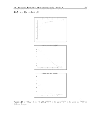
212. 198 Chapter 4. Application to a Miniature Synchronous Motor
upper domain :
*********************** Calculation of G_0,0(kappa) ***************************
--> parameter a=4.1 rho=1 m=0
--> kappa in [0, .99]
--> kappa-steps = .0396
(4*M is the size of arrays used during Discrete Fourier Transformation)
--------------------------------------------------------------------------------
| M | kappa | G_0,0(kappa)/(a/kappa) | G_0,0(kappa)/(a/kappa)^2 |
| 63 | .0396000000 | -103.9635284755 | -1.0041355433 |
| 63 | .0792000000 | -52.1233606941 | -1.0068707724 |
| 63 | .1188000000 | -34.7942190763 | -1.0081837137 |
| 63 | .1584000000 | -26.0921659205 | -1.0080485565 |
| 63 | .1980000000 | -20.8403255244 | -1.0064352326 |
| 63 | .2376000000 | -17.3129898053 | -1.0033088726 |
| 63 | .2772000000 | -14.7704882524 | -.9986291081 |
| 63 | .3168000000 | -12.8429028620 | -.9923491772 |
| 63 | .3564000000 | -11.3246368136 | -.9844147708 |
| 63 | .3960000000 | -10.0922383712 | -.9747625353 |
| 63 | .4356000000 | -9.0670436852 | -.9633181047 |
| 63 | .4752000000 | -8.1964925365 | -.9499934764 |
| 63 | .5148000000 | -7.4440601230 | -.9346834515 |
| 63 | .5544000000 | -6.7834936337 | -.9172607001 |
| 63 | .5940000000 | -6.1953398511 | -.8975687491 |
| 63 | .6336000000 | -5.6647538438 | -.8754117159 |
| 63 | .6732000000 | -5.1800487132 | -.8505387301 |
| 63 | .7128000000 | -4.7316763584 | -.8226192459 |
| 63 | .7524000000 | -4.3114396356 | -.7912017516 |
| 63 | .7920000000 | -3.9117717760 | -.7556398162 |
| 63 | .8316000000 | -3.5248715434 | -.7149471159 |
| 63 | .8712000000 | -3.1412408050 | -.6674753632 |
| 63 | .9108000000 | -2.7461676113 | -.6100510878 |
| 63 | .9504000000 | -2.3069822442 | -.5347697377 |
| 63 | .9900000000 | -1.6581837158 | -.4003907021 |
******************** CALCULATION COMPLETE *************************
******************* Detection of Resonances ***********************
2 : 1-Resonance in +.8038707404......
2 : 2-Resonance in +.9878039867......
******************* DETECTION COMPLETE ***********************
*********************** Calculation of G_-k,2(kappa)| ***************************
--> parameter a=4.1 rho=1 m=0
--> 2 : 1 Resonance in .803870
--> kappa in [.753870, .853870]
--> kappa-steps = .05
(4*M is the size of arrays used during Discrete Fourier Transformation)
-----------------------------------------------------------------------------------------
| M | kappa | G_-1,2(kappa)/(a/kappa)| | G_0,0(kappa)/(a/kappa)|| passage |
| 63 | .7538707404 | +0.0000000000 | -4.2962744771 | certain |
| 63 | .8038707404 | +0.0000000000 | -3.7948329322 | certain |
| 63 | .8538707404 | +0.0000000000 | -3.3094704714 | certain |
******************************* CALCULATION COMPLETE **********************************

213. 4.5. Numerical Evaluations, Discussion Following Chapter 2 199
*********************** Calculation of 2*|G_-k,2(kappa)| ***************************
--> parameter abar=4.1 rho=1 m=0
--> 2 : 2 Resonance in .987803
--> kappa in [.937803, .987803]
--> kappa-steps = .025
(4*M is the size of arrays used during Discrete Fourier Transformation)
-----------------------------------------------------------------------------------------
| M | kappa | G_-2,2(kappa)/(a/kappa) | G_0,0(kappa)/(a/kappa) | passage |
| 63 | .9378039867 | +1.1010778373 | -2.4553353062 | certain |
| 63 | .9628039867 | +.5373629107 | -2.1465898444 | certain |
| 63 | .9878039867 | +.3885728462 | -1.7145290398 | certain |
******************************* CALCULATION COMPLETE **********************************
central domain :
******************* Calculation of G_0,0(kappa) ***********************
--> parameter a=4.1 rho=1 m=0
--> kappa in [0, .99]
--> kappa-steps = .0396
(4*M is the size of arrays used during Discrete Fourier Transformation)
--------------------------------------------------------------------------------
| M | kappa | G_0,0(kappa)/(a*kappa) | G_0,0(kappa)/(a*kappa)^2 |
| 63 | .0396000000 | -0.0994989434 | -.6128291663 |
| 63 | .0792000000 | -0.1987133128 | -.6119527987 |
| 63 | .1188000000 | -0.2973607928 | -.6104968235 |
| 63 | .1584000000 | -0.3951635878 | -.6084682001 |
| 63 | .1980000000 | -0.4918506650 | -.6058766506 |
| 63 | .2376000000 | -0.5871599104 | -.6027345718 |
| 63 | .2772000000 | -0.6808400647 | -.5990568267 |
| 63 | .3168000000 | -0.7726522062 | -.5948603460 |
| 63 | .3564000000 | -0.8623704436 | -.5901634526 |
| 63 | .3960000000 | -0.9497813437 | -.5849848138 |
| 63 | .4356000000 | -1.0346814769 | -.5793419096 |
| 63 | .4752000000 | -1.1168722919 | -.5732488974 |
| 63 | .5148000000 | -1.1961513356 | -.5667137300 |
| 63 | .5544000000 | -1.2722985562 | -.5597343453 |
| 63 | .5940000000 | -1.3450559918 | -.5522936650 |
| 63 | .6336000000 | -1.4140983398 | -.5443529578 |
| 63 | .6732000000 | -1.4789903074 | -.5358427559 |
| 63 | .7128000000 | -1.5391232812 | -.5266497225 |
| 63 | .7524000000 | -1.5936162517 | -.5165960801 |
| 63 | .7920000000 | -1.6411466798 | -.5054036338 |
| 63 | .8316000000 | -1.6796184458 | -.4926202928 |
| 63 | .8712000000 | -1.7053376252 | -.4774288408 |
| 63 | .9108000000 | -1.7099435467 | -.4579044813 |
| 63 | .9504000000 | -1.6601301063 | -.4260414373 |
| 63 | .9900000000 | -1.3641773148 | -.3360870448 |
******************** CALCULATION COMPLETE *************************
******************* Detection of Resonances ***********************
2 : 1-Resonance in +.3075848728......
2 : 2-Resonance in +.9867635460......
******************* DETECTION COMPLETE ***********************

214. 200 Chapter 4. Application to a Miniature Synchronous Motor
******************* Calculation of G_-k,2(kappa)| ***********************
--> parameter a=4.1 rho=1 m=0
--> 2 : 1 Resonance in .307584
--> kappa in [.257584, .357584]
--> kappa-steps = .05
(4*M is the size of arrays used during Discrete Fourier Transformation)
-----------------------------------------------------------------------------------------
| M | kappa | G_-1,2(kappa)/(a*kappa) | G_0,0(kappa)/(a*kappa) | passage |
| 63 | .2575848728 | +.1614991274 | -.6346562326 | certain |
| 63 | .3075848728 | +.2323316952 | -.7514659023 | certain |
| 63 | .3575848728 | +.3173595687 | -.8650203885 | certain |
******************** CALCULATION COMPLETE *************************
******************* Calculation of 2*|G_-k,2(kappa)| ***********************
--> parameter abar=4.1 rho=1 m=0
--> 2 : 2 Resonance in .986763
--> kappa in [.936763, .986763]
--> kappa-steps = .025
(4*M is the size of arrays used during Discrete Fourier Transformation)
-----------------------------------------------------------------------------------------
| M | kappa | G_-2,2(kappa)/(a*kappa) | G_0,0(kappa)/(a*kappa) | passage |
| 63 | .9367635460 | +.1340754295 | -1.6889205617 | certain |
| 63 | .9617635460 | +.1540029415 | -1.6175647928 | certain |
| 63 | .9867635460 | +.1516329740 | -1.4111461809 | certain |
******************** CALCULATION COMPLETE *************************
lower domain :
************************** Calculation of G_0,0(kappa) ***************************
--> parameter a=4.1 rho=1 m=0
--> kappa in [0, .99]
--> kappa-steps = .0396
(4*M is the size of arrays used during Discrete Fourier Transformation)
----------------------------------------------------------------------------------
| M | kappa | G_0,0(kappa)/(-a/kappa) | G_0,0(kappa)/(-a/kappa)^2 |
| 63 | .0396000000 | +102.9641074254 | -.9944825985 |
| 63 | .0792000000 | +51.1256805330 | -.9875985117 |
| 63 | .1188000000 | +33.7994539872 | -.9793597887 |
| 63 | .1584000000 | +25.1015109210 | -.9697754463 |
| 63 | .1980000000 | +19.8550057333 | -.9588514963 |
| 63 | .2376000000 | +16.3342707219 | -.9465909081 |
| 63 | .2772000000 | +13.7996874693 | -.9329935040 |
| 63 | .3168000000 | +11.8814037494 | -.9180557823 |
| 63 | .3564000000 | +10.3739048950 | -.9017706596 |
| 63 | .3960000000 | +9.1538413796 | -.8841271186 |
| 63 | .4356000000 | +8.1426767014 | -.8651097490 |
| 63 | .4752000000 | +7.2880102489 | -.8446981634 |
| 63 | .5148000000 | +6.5535192746 | -.8228662738 |
| 63 | .5544000000 | +5.9132104045 | -.7995814264 |
| 63 | .5940000000 | +5.3479698130 | -.7748034314 |
| 63 | .6336000000 | +4.8434072866 | -.7484836236 |
| 63 | .6732000000 | +4.3884638371 | -.7205643549 |
| 63 | .7128000000 | +3.9744921582 | -.6909800025 |
| 63 | .7524000000 | +3.5946514947 | -.6596623864 |
| 63 | .7920000000 | +3.2435474970 | -.6265584433 |
| 63 | .8316000000 | +2.9171399311 | -.5916813577 |
| 63 | .8712000000 | +2.6130509022 | -.5552414502 |
| 63 | .9108000000 | +2.3304129569 | -.5176927124 |
| 63 | .9504000000 | +2.0336280953 | -.4714049126 |
| 63 | .9900000000 | +1.2319443416 | -.2974694873 |
******************** CALCULATION COMPLETE *************************

215. 4.5. Numerical Evaluations, Discussion Following Chapter 2 201
******************* Detection of Resonances ***********************
2 : 1-Resonance in +.8038707404......
2 : 2-Resonance in +.9878039867......
******************* DETECTION COMPLETE ***********************
******************* Calculation of G_-k,2(kappa)| ***********************
--> parameter a=4.1 rho=1 m=0
--> 2 : 1 Resonance in .803870
--> kappa in [.753870, .853870]
--> kappa-steps = .05
(4*M is the size of arrays used during Discrete Fourier Transformation)
-------------------------------------------------------------------------------------------
| M | kappa | G_-1,2(kappa)/(-a/kappa) | G_0,0(kappa)/(-a/kappa) | passage |
| 63 | .7538707404 | +0.0000000000 | +3.5811268746 | certain |
| 63 | .8038707404 | +0.0000000000 | +3.1432550380 | certain |
| 63 | .8538707404 | +0.0000000000 | +2.7434415410 | certain |
******************** CALCULATION COMPLETE *************************
******************* Calculation of 2*|G_-k,2(kappa)| ***********************
--> parameter abar=4.1 rho=1 m=0
--> 2 : 2 Resonance in .987803
--> kappa in [.937803, .987803]
--> kappa-steps = .025
(4*M is the size of arrays used during Discrete Fourier Transformation)
-------------------------------------------------------------------------------------------
| M | kappa | G_-2,2(kappa)/(-a/kappa) | G_0,0(kappa)/(-a/kappa) | passage |
| 63 | .9378039867 | -1.3260918711 | +2.1403696584 | certain |
| 63 | .9628039867 | -.7919794060 | +1.8811404240 | certain |
| 63 | .9878039867 | -.1268307864 | +1.2949954190 | certain |
******************** CALCULATION COMPLETE *************************
Since ̺ is sufficiently large all solutions pass through the resonances appear-
P
P=-1
Q
Figure 4.29: a = 4.1,
̺ = 1, m = 0
ing in each of the three domains. The solutions of the upper and lower
domains tend towards the separatrices while the periodic solution near the
origin is globally attractive on the central domain.

216. 202 Chapter 4. Application to a Miniature Synchronous Motor
4.5.6 a = 4.1, ̺ = 0, m = 1
-0.58
-0.56
-0.54
-0.52
-0.5
-0.48
-0.46
-0.44
-0.42
-0.4
0.2 0.4 0.6 0.8 1
G_0,0(kappa) ( abar=4.1 , rho=0 , m=1.0 , M=63)
-0.24
-0.22
-0.2
-0.18
-0.16
-0.14
-0.12
-0.1
-0.08
-0.06
-0.04
-0.02
0.2 0.4 0.6 0.8 1
G_0,0(kappa) ( abar=4.1 , rho=0 , m=1. , M=63)
-0.5
-0.4
-0.3
-0.2
-0.1
0
0.1
0.2
0.2 0.4 0.6 0.8 1
G_0,0(kappa) ( abar=4.1 , rho=0 , m=1. , M=63)
Figure 4.30: a = 4.1, ̺ = 0, m = 1 : plot of
G0,0(κ)
a/κ on the upper,
G0,0(κ)
a κ on the central and
G0,0(κ)
−a/κ on
the lower domains

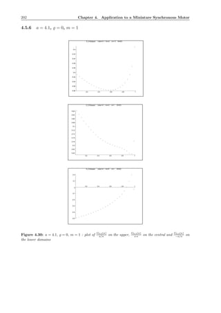
217. 4.5. Numerical Evaluations, Discussion Following Chapter 2 203
upper domain :
*********************** Calculation of G_0,0(kappa) ***************************
--> parameter a=4.1 rho=0 m=1
--> kappa in [0, .99]
--> kappa-steps = .0396
(4*M is the size of arrays used during Discrete Fourier Transformation)
--------------------------------------------------------------------------------
| M | kappa | G_0,0(kappa)/(a/kappa) | G_0,0(kappa)/(a/kappa)^2 |
| 63 | .0396000000 | -.5093708655 | -.0049197771 |
| 63 | .0792000000 | -.5181716306 | -.0100095593 |
| 63 | .1188000000 | -.5264072726 | -.0152529717 |
| 63 | .1584000000 | -.5340789481 | -.0206336842 |
| 63 | .1980000000 | -.5411839286 | -.0261352238 |
| 63 | .2376000000 | -.5477154156 | -.0317407762 |
| 63 | .2772000000 | -.5536622177 | -.0374329675 |
| 63 | .3168000000 | -.5590082671 | -.0431936144 |
| 63 | .3564000000 | -.5637319317 | -.0490034293 |
| 63 | .3960000000 | -.5678050632 | -.0548416597 |
| 63 | .4356000000 | -.5711916907 | -.0606856342 |
| 63 | .4752000000 | -.5738462196 | -.0665101764 |
| 63 | .5148000000 | -.5757109237 | -.0722868252 |
| 63 | .5544000000 | -.5767123950 | -.0779827687 |
| 63 | .5940000000 | -.5767564018 | -.0835593421 |
| 63 | .6336000000 | -.5757202320 | -.0889698387 |
| 63 | .6732000000 | -.5734408836 | -.0941561958 |
| 63 | .7128000000 | -.5696960500 | -.0990437425 |
| 63 | .7524000000 | -.5641718105 | -.1035324073 |
| 63 | .7920000000 | -.5564038250 | -.1074809340 |
| 63 | .8316000000 | -.5456601563 | -.1106758502 |
| 63 | .8712000000 | -.5306765473 | -.1127622946 |
| 63 | .9108000000 | -.5089345715 | -.1130579531 |
| 63 | .9504000000 | -.4739216366 | -.1098573471 |
| 63 | .9900000000 | -.3892378791 | -.0939867073 |
******************** CALCULATION COMPLETE *************************
******************* Detection of Resonances ***********************
2 : 1-Resonance in +.8038707404......
2 : 2-Resonance in +.9878039867......
******************* DETECTION COMPLETE ***********************
*********************** Calculation of G_-k,2(kappa)| ***************************
--> parameter a=4.1 rho=0 m=1
--> 2 : 1 Resonance in .803870
--> kappa in [.753870, .853870]
--> kappa-steps = .05
(4*M is the size of arrays used during Discrete Fourier Transformation)
-----------------------------------------------------------------------------------------
| M | kappa | G_-1,2(kappa)/(a/kappa) | G_0,0(kappa)/(a/kappa) | passage |
| 63 | .7538707404 | +0.0000000000 | -.5639269391 | certain |
| 63 | .8038707404 | +0.0000000000 | -.5535391662 | certain |
| 63 | .8538707404 | +0.0000000000 | -.5378728793 | certain |
******************************* CALCULATION COMPLETE **********************************

218. 204 Chapter 4. Application to a Miniature Synchronous Motor
*********************** Calculation of 2*|G_-k,2(kappa)| ***************************
--> parameter abar=4.1 rho=0 m=1
--> 2 : 2 Resonance in .987803
--> kappa in [.937803, .987803]
--> kappa-steps = .025
(4*M is the size of arrays used during Discrete Fourier Transformation)
-----------------------------------------------------------------------------------------
| M | kappa | G_-2,2(kappa)/(a/kappa) | G_0,0(kappa)/(a/kappa) | passage |
| 63 | .9378039867 | +1.1010778373 | -.4873089776 | mostly |
| 63 | .9628039867 | +.5373629107 | -.4572925441 | mostly |
| 63 | .9878039867 | +.3885728462 | -.3985989415 | certain |
******************************* CALCULATION COMPLETE **********************************
central domain :
******************* Calculation of G_0,0(kappa) ***********************
--> parameter a=4.1 rho=0 m=1
--> kappa in [0, .99]
--> kappa-steps = .0396
(4*M is the size of arrays used during Discrete Fourier Transformation)
--------------------------------------------------------------------------------
| M | kappa | G_0,0(kappa)/(a*kappa) | G_0,0(kappa)/(a*kappa)^2 |
| 63 | .0396000000 | -.0183348688 | -.1129272532 |
| 63 | .0792000000 | -.0364810169 | -.1123460733 |
| 63 | .1188000000 | -.0542535008 | -.1113851950 |
| 63 | .1584000000 | -.0714749993 | -.1100563551 |
| 63 | .1980000000 | -.0879797762 | -.1083761718 |
| 63 | .2376000000 | -.1036177765 | -.1063662812 |
| 63 | .2772000000 | -.1182588207 | -.1040534445 |
| 63 | .3168000000 | -.1317968033 | -.1014695763 |
| 63 | .3564000000 | -.1441537322 | -.0986516467 |
| 63 | .3960000000 | -.1552833893 | -.0956414075 |
| 63 | .4356000000 | -.1651743492 | -.0924849096 |
| 63 | .4752000000 | -.1738521029 | -.0892318012 |
| 63 | .5148000000 | -.1813801006 | -.0859344384 |
| 63 | .5544000000 | -.1878597129 | -.0826469014 |
| 63 | .5940000000 | -.1934294449 | -.0794240966 |
| 63 | .6336000000 | -.1982643239 | -.0763212629 |
| 63 | .6732000000 | -.2025773916 | -.0733944146 |
| 63 | .7128000000 | -.2066270581 | -.0707026423 |
| 63 | .7524000000 | -.2107375600 | -.0683139352 |
| 63 | .7920000000 | -.2153464056 | -.0663175676 |
| 63 | .8316000000 | -.2211019890 | -.0648476604 |
| 63 | .8712000000 | -.2290058009 | -.0641128023 |
| 63 | .9108000000 | -.2399676172 | -.0642607456 |
| 63 | .9504000000 | -.2444025627 | -.0627213606 |
| 63 | .9900000000 | -.1776456195 | -.0437658584 |
******************** CALCULATION COMPLETE *************************
******************* Detection of Resonances ***********************
2 : 1-Resonance in +.3075848728......
2 : 2-Resonance in +.9867635460......
******************* DETECTION COMPLETE ***********************

219. 4.5. Numerical Evaluations, Discussion Following Chapter 2 205
******************* Calculation of G_-k,2(kappa)| ***********************
--> parameter a=4.1 rho=0 m=1
--> 2 : 1 Resonance in .307584
--> kappa in [.257584, .357584]
--> kappa-steps = .05
(4*M is the size of arrays used during Discrete Fourier Transformation)
-----------------------------------------------------------------------------------------
| M | kappa | G_-1,2(kappa)/(a*kappa) | G_0,0(kappa)/(a*kappa) | passage |
| 63 | .2575848728 | +.1614991274 | -.1111385236 | mostly |
| 63 | .3075848728 | +.2323316952 | -.1287495137 | mostly |
| 63 | .3575848728 | +.3173595687 | -.1445046992 | mostly |
******************** CALCULATION COMPLETE *************************
******************* Calculation of 2*|G_-k,2(kappa)| ***********************
--> parameter abar=4.1 rho=0 m=1
--> 2 : 2 Resonance in .986763
--> kappa in [.936763, .986763]
--> kappa-steps = .025
(4*M is the size of arrays used during Discrete Fourier Transformation)
-----------------------------------------------------------------------------------------
| M | kappa | G_-2,2(kappa)/(a*kappa) | G_0,0(kappa)/(a*kappa) | passage |
| 63 | .9367635460 | +.1340754295 | -.2461359773 | certain |
| 63 | .9617635460 | +.1540029415 | -.2354069917 | certain |
| 63 | .9867635460 | +.1516329740 | -.1838326901 | certain |
******************** CALCULATION COMPLETE *************************
lower domain :
************************** Calculation of G_0,0(kappa) ***************************
--> parameter a=4.1 rho=0 m=1
--> kappa in [0, .99]
--> kappa-steps = .0396
(4*M is the size of arrays used during Discrete Fourier Transformation)
----------------------------------------------------------------------------------
| M | kappa | G_0,0(kappa)/(-a/kappa) | G_0,0(kappa)/(-a/kappa)^2 |
| 63 | .0396000000 | -.4900501845 | +.0047331676 |
| 63 | .0792000000 | -.4795085305 | +.0092627013 |
| 63 | .1188000000 | -.4683578165 | +.0135709533 |
| 63 | .1584000000 | -.4565760513 | +.0176394259 |
| 63 | .1980000000 | -.4441358623 | +.0214485123 |
| 63 | .2376000000 | -.4310036677 | +.0249771881 |
| 63 | .2772000000 | -.4171385653 | +.0282026366 |
| 63 | .3168000000 | -.4024908454 | +.0310997804 |
| 63 | .3564000000 | -.3869999868 | +.0336406817 |
| 63 | .3960000000 | -.3705919282 | +.0357937569 |
| 63 | .4356000000 | -.3531752930 | +.0375227213 |
| 63 | .4752000000 | -.3346360680 | +.0387851364 |
| 63 | .5148000000 | -.3148299246 | +.0395303524 |
| 63 | .5544000000 | -.2935708342 | +.0396965049 |
| 63 | .5940000000 | -.2706136362 | +.0392059755 |
| 63 | .6336000000 | -.2456263252 | +.0379582535 |
| 63 | .6732000000 | -.2181439924 | +.0358181794 |
| 63 | .7128000000 | -.1874881501 | +.0325955008 |
| 63 | .7524000000 | -.1526163304 | +.0280069578 |
| 63 | .7920000000 | -.1118204539 | +.0216004389 |
| 63 | .8316000000 | -.0620714559 | +.0125899079 |
| 63 | .8712000000 | +.0024866445 | -.0005283816 |
| 63 | .9108000000 | +.0931799172 | -.0206995777 |
| 63 | .9504000000 | +.2005674876 | -.0464925220 |
| 63 | .9900000000 | -.0370014950 | +.0089345073 |
******************** CALCULATION COMPLETE *************************

220. 206 Chapter 4. Application to a Miniature Synchronous Motor
******************* Detection of Resonances ***********************
2 : 1-Resonance in +.8038707404......
2 : 2-Resonance in +.9878039867......
******************* DETECTION COMPLETE ***********************
******************* Calculation of G_-k,2(kappa)| ***********************
--> parameter a=4.1 rho=0 m=1
--> 2 : 1 Resonance in .803870
--> kappa in [.753870, .853870]
--> kappa-steps = .05
(4*M is the size of arrays used during Discrete Fourier Transformation)
-------------------------------------------------------------------------------------------
| M | kappa | G_-1,2(kappa)/(-a/kappa) | G_0,0(kappa)/(-a/kappa) | passage |
| 63 | .7538707404 | +0.0000000000 | -.1512206632 | certain |
| 63 | .8038707404 | +0.0000000000 | -.0980387279 | certain |
| 63 | .8538707404 | +0.0000000000 | -.0281560509 | certain |
******************** CALCULATION COMPLETE *************************
******************* Calculation of 2*|G_-k,2(kappa)| ***********************
--> parameter abar=4.1 rho=0 m=1
--> 2 : 2 Resonance in .987803
--> kappa in [.937803, .987803]
--> kappa-steps = .025
(4*M is the size of arrays used during Discrete Fourier Transformation)
-------------------------------------------------------------------------------------------
| M | kappa | G_-2,2(kappa)/(-a/kappa) | G_0,0(kappa)/(-a/kappa) | passage |
| 63 | .9378039867 | -1.3260918711 | +.1723433298 | mostly |
| 63 | .9628039867 | -.7919794060 | +.1918431237 | mostly |
| 63 | .9878039867 | -.1268307864 | -.0209346791 | mostly |
******************** CALCULATION COMPLETE *************************
The situation is qualitatively equivalent to the one observed in section 4.5.4
P
P=-1
Q
Figure 4.31: a = 4.1,
̺ = 0, m = 1
for ̺ = 0, m = 0. A passage up to a O(ε) set, however, arises in the 2 : 2
resonance at κkm ≈ 0.98 situated close to the lower separatrix here.

221. 4.5. Numerical Evaluations, Discussion Following Chapter 2 207
4.5.7 a = 20.38, ̺ = 0, m = 0
-0.04
-0.035
-0.03
-0.025
-0.02
-0.015
-0.01
-0.005
0.2 0.4 0.6 0.8 1
G_0,0(kappa) ( abar=20.38 , rho=0 , m=0 , M=63)
-0.05
-0.04
-0.03
-0.02
-0.01
0.2 0.4 0.6 0.8 1
G_0,0(kappa) ( abar=20.38 , rho=0 , m=0 , M=63)
0.01
0.02
0.03
0.04
0.2 0.4 0.6 0.8 1
G_0,0(kappa) ( abar=20.38 , rho=0 , m=0 , M=63)
Figure 4.32: a = 20.38, ̺ = 0, m = 0 : plot of
G0,0(κ)
a/κ on the upper,
G0,0(κ)
a κ on the central and
G0,0(κ)
−a/κ
on the lower domains

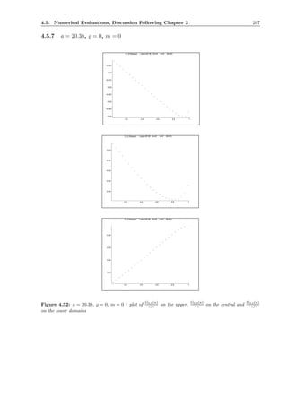
222. 208 Chapter 4. Application to a Miniature Synchronous Motor
upper domain :
*********************** Calculation of G_0,0(kappa) ***************************
--> parameter a=20.38 rho=0 m=0
--> kappa in [0, .99]
--> kappa-steps = .0396
(4*M is the size of arrays used during Discrete Fourier Transformation)
--------------------------------------------------------------------------------
| M | kappa | G_0,0(kappa)/(a/kappa) | G_0,0(kappa)/(a/kappa)^2 |
| 63 | .0396000000 | -.0019393189 | -.0000037682 |
| 63 | .0792000000 | -.0038711513 | -.0000150439 |
| 63 | .1188000000 | -.0057955195 | -.0000337834 |
| 63 | .1584000000 | -.0077123913 | -.0000599432 |
| 63 | .1980000000 | -.0096216679 | -.0000934784 |
| 63 | .2376000000 | -.0115231695 | -.0001343427 |
| 63 | .2772000000 | -.0134166167 | -.0001824870 |
| 63 | .3168000000 | -.0153016055 | -.0002378581 |
| 63 | .3564000000 | -.0171775757 | -.0003003968 |
| 63 | .3960000000 | -.0190437667 | -.0003700358 |
| 63 | .4356000000 | -.0208991584 | -.0004466964 |
| 63 | .4752000000 | -.0227423881 | -.0005302837 |
| 63 | .5148000000 | -.0245716332 | -.0006206809 |
| 63 | .5544000000 | -.0263844401 | -.0007177396 |
| 63 | .5940000000 | -.0281774695 | -.0008212667 |
| 63 | .6336000000 | -.0299461040 | -.0009310035 |
| 63 | .6732000000 | -.0316838219 | -.0010465921 |
| 63 | .7128000000 | -.0333811511 | -.0011675213 |
| 63 | .7524000000 | -.0350238227 | -.0012930286 |
| 63 | .7920000000 | -.0365892724 | -.0014219187 |
| 63 | .8316000000 | -.0380393704 | -.0015521854 |
| 63 | .8712000000 | -.0393032314 | -.0016801263 |
| 63 | .9108000000 | -.0402279060 | -.0017978202 |
| 63 | .9504000000 | -.0403803780 | -.0018830967 |
| 63 | .9900000000 | -.0370744636 | -.0018009675 |
******************** CALCULATION COMPLETE *************************
******************* Detection of Resonances ***********************
******************* DETECTION COMPLETE ***********************
central domain :
******************* Calculation of G_0,0(kappa) ***********************
--> parameter a=20.38 rho=0 m=0
--> kappa in [0, .99]
--> kappa-steps = .0396
(4*M is the size of arrays used during Discrete Fourier Transformation)
--------------------------------------------------------------------------------
| M | kappa | G_0,0(kappa)/(a*kappa) | G_0,0(kappa)/(kappa*a)^2 |
| 63 | .0396000000 | -.0039625525 | -.0049099341 |
| 63 | .0792000000 | -.0079113463 | -.0049014100 |
| 63 | .1188000000 | -.0118325499 | -.0048871731 |
| 63 | .1584000000 | -.0157121835 | -.0048671775 |
| 63 | .1980000000 | -.0195360393 | -.0048413574 |
| 63 | .2376000000 | -.0232895935 | -.0048096258 |
| 63 | .2772000000 | -.0269579065 | -.0047718717 |
| 63 | .3168000000 | -.0305255085 | -.0047279573 |
| 63 | .3564000000 | -.0339762616 | -.0046777145 |
| 63 | .3960000000 | -.0372931942 | -.0046209388 |
| 63 | .4356000000 | -.0404582925 | -.0045573827 |
| 63 | .4752000000 | -.0434522354 | -.0044867462 |
| 63 | .5148000000 | -.0462540484 | -.0044086643 |
| 63 | .5544000000 | -.0488406378 | -.0043226883 |
| 63 | .5940000000 | -.0511861489 | -.0042282614 |

223. 4.5. Numerical Evaluations, Discussion Following Chapter 2 209
| 63 | .6336000000 | -.0532610487 | -.0041246809 |
| 63 | .6732000000 | -.0550307682 | -.0040110427 |
| 63 | .7128000000 | -.0564535952 | -.0038861515 |
| 63 | .7524000000 | -.0574772234 | -.0037483731 |
| 63 | .7920000000 | -.0580326839 | -.0035953675 |
| 63 | .8316000000 | -.0580226497 | -.0034235675 |
| 63 | .8712000000 | -.0572958240 | -.0032270145 |
| 63 | .9108000000 | -.0555790142 | -.0029942195 |
| 63 | .9504000000 | -.0522260064 | -.0026963496 |
| 63 | .9900000000 | -.0439543128 | -.0021785228 |
******************** CALCULATION COMPLETE *************************
******************* Detection of Resonances ***********************
******************* DETECTION COMPLETE ***********************
lower domain :
************************** Calculation of G_0,0(kappa) ***************************
--> parameter a=20.38 rho=0 m=0
--> kappa in [0, .99]
--> kappa-steps = .0396
(4*M is the size of arrays used during Discrete Fourier Transformation)
----------------------------------------------------------------------------------
| M | kappa | G_0,0(kappa)/(-a/kappa) | G_0,0(kappa)/(-a/kappa)^2 |
| 63 | .0396000000 | +.0019468731 | -.0000037829 |
| 63 | .0792000000 | +.0039014051 | -.0000151614 |
| 63 | .1188000000 | +.0058637304 | -.0000341811 |
| 63 | .1584000000 | +.0078340060 | -.0000608884 |
| 63 | .1980000000 | +.0098124046 | -.0000953315 |
| 63 | .2376000000 | +.0117991063 | -.0001375597 |
| 63 | .2772000000 | +.0137942889 | -.0001876239 |
| 63 | .3168000000 | +.0157981158 | -.0002455762 |
| 63 | .3564000000 | +.0178107192 | -.0003114691 |
| 63 | .3960000000 | +.0198321780 | -.0003853553 |
| 63 | .4356000000 | +.0218624855 | -.0004672864 |
| 63 | .4752000000 | +.0239015033 | -.0005573108 |
| 63 | .5148000000 | +.0259488925 | -.0006554705 |
| 63 | .5544000000 | +.0280040098 | -.0007617970 |
| 63 | .5940000000 | +.0300657458 | -.0008763028 |
| 63 | .6336000000 | +.0321322654 | -.0009989697 |
| 63 | .6732000000 | +.0342005769 | -.0011297266 |
| 63 | .7128000000 | +.0362657837 | -.0012684126 |
| 63 | .7524000000 | +.0383197137 | -.0014147081 |
| 63 | .7920000000 | +.0403482266 | -.0015679978 |
| 63 | .8316000000 | +.0423254104 | -.0017270761 |
| 63 | .8712000000 | +.0441993543 | -.0018894248 |
| 63 | .9108000000 | +.0458497570 | -.0020490656 |
| 63 | .9504000000 | +.0469103056 | -.0021876130 |
| 63 | .9900000000 | +.0448817581 | -.0021802227 |
******************** CALCULATION COMPLETE *************************
******************* Detection of Resonances ***********************
******************* DETECTION COMPLETE ***********************

224. 210 Chapter 4. Application to a Miniature Synchronous Motor
4.5.8 a = 20.38, ̺ = 1, m = 0
-500
-400
-300
-200
-100
0
0.2 0.4 0.6 0.8 1
G_0,0(kappa) ( abar=20.38 , rho=1.0 , m=0 , M=63)
-7
-6
-5
-4
-3
-2
-1
0.2 0.4 0.6 0.8 1
G_0,0(kappa) ( abar=20.38 , rho=1.0 , m=0 , M=63)
0
100
200
300
400
500
0.2 0.4 0.6 0.8 1
G_0,0(kappa) ( abar=20.38 , rho=1.0 , m=0 , M=63)
Figure 4.33: a = 20.38, ̺ = 1, m = 0 : plot of
G0,0(κ)
a/κ on the upper,
G0,0(κ)
a κ on the central and
G0,0(κ)
−a/κ
on the lower domains

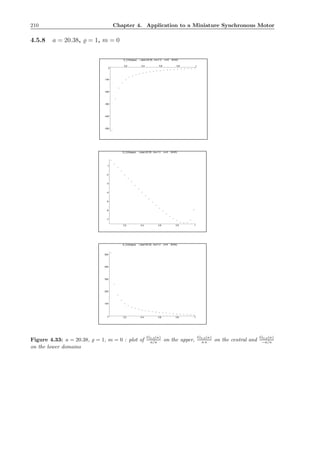
225. 4.5. Numerical Evaluations, Discussion Following Chapter 2 211
upper domain :
*********************** Calculation of G_0,0(kappa) ***************************
--> parameter a=20.38 rho=1 m=0
--> kappa in [0, .99]
--> kappa-steps = .0396
(4*M is the size of arrays used during Discrete Fourier Transformation)
--------------------------------------------------------------------------------
| M | kappa | G_0,0(kappa)/(a/kappa) | G_0,0(kappa)/(a/kappa)^2 |
| 63 | .0396000000 | -514.7446046884 | -1.0001906940 |
| 63 | .0792000000 | -257.0186350694 | -.9988162854 |
| 63 | .1188000000 | -170.8401221711 | -.9958688181 |
| 63 | .1584000000 | -127.5469444271 | -.9913364081 |
| 63 | .1980000000 | -101.4062465628 | -.9852029842 |
| 63 | .2376000000 | -83.8400189303 | -.9774479145 |
| 63 | .2772000000 | -71.1715986696 | -.9680454931 |
| 63 | .3168000000 | -61.5622839303 | -.9569642565 |
| 63 | .3564000000 | -53.9901926624 | -.9441660777 |
| 63 | .3960000000 | -47.8417911655 | -.9296049706 |
| 63 | .4356000000 | -42.7262068503 | -.9132255006 |
| 63 | .4752000000 | -38.3823612383 | -.8949606506 |
| 63 | .5148000000 | -34.6289339413 | -.8747289103 |
| 63 | .5544000000 | -31.3357289214 | -.8524302313 |
| 63 | .5940000000 | -28.4064354584 | -.8279402680 |
| 63 | .6336000000 | -25.7677675539 | -.8011019392 |
| 63 | .6732000000 | -23.3623042177 | -.7717126201 |
| 63 | .7128000000 | -21.1435022902 | -.7395038485 |
| 63 | .7524000000 | -19.0719149710 | -.7041074005 |
| 63 | .7920000000 | -17.1118553878 | -.6649945764 |
| 63 | .8316000000 | -15.2275872507 | -.6213572893 |
| 63 | .8712000000 | -13.3771627036 | -.5718441681 |
| 63 | .9108000000 | -11.4979629262 | -.5138540055 |
| 63 | .9504000000 | -9.4548429811 | -.4409167207 |
| 63 | .9900000000 | -6.5786499577 | -.3195713178 |
******************** CALCULATION COMPLETE *************************
******************* Detection of Resonances ***********************
******************* DETECTION COMPLETE ***********************
central domain :
******************* Calculation of G_0,0(kappa) ***********************
--> parameter a=20.38 rho=1 m=0
--> kappa in [0, .99]
--> kappa-steps = .0396
(4*M is the size of arrays used during Discrete Fourier Transformation)
--------------------------------------------------------------------------------
| M | kappa | G_0,0(kappa)/(a*kappa) | G_0,0(kappa)/(kappa*a)^2 |
| 63 | .0396000000 | -0.4074073917 | -.5048118472 |
| 63 | .0792000000 | -0.8143245635 | -.5045081355 |
| 63 | .1188000000 | -1.2202536745 | -.5039988016 |
| 63 | .1584000000 | -1.6246813141 | -.5032790224 |
| 63 | .1980000000 | -2.0270698716 | -.5023418363 |
| 63 | .2376000000 | -2.4268478103 | -.5011779163 |
| 63 | .2772000000 | -2.8233983338 | -.4997752539 |
| 63 | .3168000000 | -3.2160457796 | -.4981187270 |
| 63 | .3564000000 | -3.6040388413 | -.4961895205 |
| 63 | .3960000000 | -3.9865293677 | -.4939643450 |
| 63 | .4356000000 | -4.3625449417 | -.4914143826 |
| 63 | .4752000000 | -4.7309525895 | -.4885038425 |
| 63 | .5148000000 | -5.0904096020 | -.4851879558 |
| 63 | .5544000000 | -5.4392951812 | -.4814101322 |
| 63 | .5940000000 | -5.7756127408 | -.4770978298 |

226. 212 Chapter 4. Application to a Miniature Synchronous Motor
| 63 | .6336000000 | -6.0968457423 | -.4721563759 |
| 63 | .6732000000 | -6.3997369203 | -.4664593840 |
| 63 | .7128000000 | -6.6799348211 | -.4598332318 |
| 63 | .7524000000 | -6.9313961838 | -.4520305179 |
| 63 | .7920000000 | -7.1453033150 | -.4426814337 |
| 63 | .8316000000 | -7.3079166473 | -.4311962000 |
| 63 | .8712000000 | -7.3957452335 | -.4165430530 |
| 63 | .9108000000 | -7.3624349761 | -.3966379552 |
| 63 | .9504000000 | -7.0894277966 | -.3660164263 |
| 63 | .9900000000 | -5.9418850324 | -.2944997091 |
******************** CALCULATION COMPLETE *************************
******************* Detection of Resonances ***********************
******************* DETECTION COMPLETE ***********************
lower domain :
************************** Calculation of G_0,0(kappa) ***************************
--> parameter a=20.38 rho=1 m=0
--> kappa in [0, .99]
--> kappa-steps = .0396
(4*M is the size of arrays used during Discrete Fourier Transformation)
----------------------------------------------------------------------------------
| M | kappa | G_0,0(kappa)/(-a/kappa) | G_0,0(kappa)/(-a/kappa)^2 |
| 63 | .0396000000 | +513.7450044749 | -.9982483894 |
| 63 | .0792000000 | +256.0202365678 | -.9949363462 |
| 63 | .1188000000 | +169.8437344256 | -.9900606305 |
| 63 | .1584000000 | +126.5533885546 | -.9836141681 |
| 63 | .1980000000 +100.4163610328 | -.9755858432 |
| 63 | .2376000000 | +82.8546653279 | -.9659601806 |
| 63 | .2772000000 | +70.1916681324 | -.9547168992 |
| 63 | .3168000000 | +60.5887044950 | -.9418303034 |
| 63 | .3564000000 | +53.0239378244 | -.9272684710 |
| 63 | .3960000000 | +46.8838900555 | -.9109921718 |
| 63 | .4356000000 | +41.7777565731 | -.8929534231 |
| 63 | .4752000000 | +37.4445421356 | -.8730935438 |
| 63 | .5148000000 | +33.7030288680 | -.8513404936 |
| 63 | .5544000000 | +30.4231481363 | -.8276051681 |
| 63 | .5940000000 | +27.5087495603 | -.8017761157 |
| 63 | .6336000000 | +24.8867522833 | -.7737117883 |
| 63 | .6732000000 | +22.5000033848 | -.7432287673 |
| 63 | .7128000000 | +20.3023196126 | -.7100830922 |
| 63 | .7524000000 | +18.2547545543 | -.6739390248 |
| 63 | .7920000000 | +16.3223498381 | -.6343131046 |
| 63 | .8316000000 | +14.4704985392 | -.5904645036 |
| 63 | .8712000000 | +12.6591689417 | -.5411515202 |
| 63 | .9108000000 | +10.8294851515 | -.4839791499 |
| 63 | .9504000000 | +8.8557526701 | -.4129787702 |
| 63 | .9900000000 | +6.1184848749 | -.2972178619 |
******************** CALCULATION COMPLETE *************************
******************* Detection of Resonances ***********************
******************* DETECTION COMPLETE ***********************

227. 4.5. Numerical Evaluations, Discussion Following Chapter 2 213
4.5.9 a = 20.38, ̺ = 0, m = 1
-0.5
-0.45
-0.4
-0.35
-0.3
0.2 0.4 0.6 0.8 1
G_0,0(kappa) ( abar=20.38 , rho=0 , m=1. , M=63)
-0.05
-0.04
-0.03
-0.02
-0.01
0.2 0.4 0.6 0.8 1
G_0,0(kappa) ( abar=20.38 , rho=0 , m=1. , M=63)
-0.5
-0.45
-0.4
-0.35
-0.3
-0.25
-0.2
0.2 0.4 0.6 0.8 1
G_0,0(kappa) ( abar=20.38 , rho=0 , m=1. , M=63)
Figure 4.34: a = 20.38, ̺ = 0, m = 1 : plot of
G0,0(κ)
a/κ on the upper,
G0,0(κ)
a κ on the central and
G0,0(κ)
−a/κ
on the lower domains

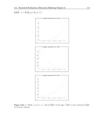
228. 214 Chapter 4. Application to a Miniature Synchronous Motor
upper domain :
*********************** Calculation of G_0,0(kappa) ***************************
--> parameter a=20.38 rho=0 m=1
--> kappa in [0, .99]
--> kappa-steps = .0396
(4*M is the size of arrays used during Discrete Fourier Transformation)
--------------------------------------------------------------------------------
| M | kappa | G_0,0(kappa)/(a/kappa) | G_0,0(kappa)/(a/kappa)^2 |
| 63 | .0396000000 | -.5017432028 | -.0009749279 |
| 63 | .0792000000 | -.5030855290 | -.0019550723 |
| 63 | .1188000000 | -.5040234977 | -.0029380761 |
| 63 | .1584000000 | -.5045511349 | -.0039215358 |
| 63 | .1980000000 | -.5046598013 | -.0049029754 |
| 63 | .2376000000 | -.5043379391 | -.0058798181 |
| 63 | .2772000000 | -.5035707214 | -.0068493525 |
| 63 | .3168000000 | -.5023395783 | -.0078086937 |
| 63 | .3564000000 | -.5006215664 | -.0087547363 |
| 63 | .3960000000 | -.4983885273 | -.0096840950 |
| 63 | .4356000000 | -.4956059605 | -.0105930302 |
| 63 | .4752000000 | -.4922314970 | -.0114773507 |
| 63 | .5148000000 | -.4882127995 | -.0123322840 |
| 63 | .5544000000 | -.4834846175 | -.0131522999 |
| 63 | .5940000000 | -.4779645567 | -.0139308609 |
| 63 | .6336000000 | -.4715468200 | -.0146600620 |
| 63 | .6732000000 | -.4640926158 | -.0153300858 |
| 63 | .7128000000 | -.4554148062 | -.0159283451 |
| 63 | .7524000000 | -.4452519765 | -.0164380562 |
| 63 | .7920000000 | -.4332215243 | -.0168356941 |
| 63 | .8316000000 | -.4187267462 | -.0170860236 |
| 63 | .8712000000 | -.4007481738 | -.0171310995 |
| 63 | .9108000000 | -.3772777189 | -.0168608707 |
| 63 | .9504000000 | -.3431904973 | -.0160043301 |
| 63 | .9900000000 | -.2710606523 | -.0131673231 |
******************** CALCULATION COMPLETE *************************
******************* Detection of Resonances ***********************
******************* DETECTION COMPLETE ***********************
central domain :
******************* Calculation of G_0,0(kappa) ***********************
--> parameter a=20.38 rho=0 m=1
--> kappa in [0, .99]
--> kappa-steps = .0396
(4*M is the size of arrays used during Discrete Fourier Transformation)
--------------------------------------------------------------------------------
| M | kappa | G_0,0(kappa)/(a*kappa) | G_0,0(kappa)/(kappa*a)^2 |
| 63 | .0396000000 | -.0039625525 | -.0049099341 |
| 63 | .0792000000 | -.0079113463 | -.0049014100 |
| 63 | .1188000000 | -.0118325499 | -.0048871731 |
| 63 | .1584000000 | -.0157121835 | -.0048671775 |
| 63 | .1980000000 | -.0195360393 | -.0048413574 |
| 63 | .2376000000 | -.0232895935 | -.0048096258 |
| 63 | .2772000000 | -.0269579065 | -.0047718717 |
| 63 | .3168000000 | -.0305255085 | -.0047279573 |
| 63 | .3564000000 | -.0339762616 | -.0046777145 |
| 63 | .3960000000 | -.0372931942 | -.0046209388 |
| 63 | .4356000000 | -.0404582925 | -.0045573827 |
| 63 | .4752000000 | -.0434522354 | -.0044867462 |
| 63 | .5148000000 | -.0462540484 | -.0044086643 |
| 63 | .5544000000 | -.0488406378 | -.0043226883 |
| 63 | .5940000000 | -.0511861489 | -.0042282614 |

229. 4.5. Numerical Evaluations, Discussion Following Chapter 2 215
| 63 | .6336000000 | -.0532610487 | -.0041246809 |
| 63 | .6732000000 | -.0550307682 | -.0040110427 |
| 63 | .7128000000 | -.0564535952 | -.0038861515 |
| 63 | .7524000000 | -.0574772234 | -.0037483731 |
| 63 | .7920000000 | -.0580326839 | -.0035953675 |
| 63 | .8316000000 | -.0580226497 | -.0034235675 |
| 63 | .8712000000 | -.0572958240 | -.0032270145 |
| 63 | .9108000000 | -.0555790142 | -.0029942195 |
| 63 | .9504000000 | -.0522260064 | -.0026963496 |
| 63 | .9900000000 | -.0439543128 | -.0021785228 |
******************** CALCULATION COMPLETE *************************
******************* Detection of Resonances ***********************
******************* DETECTION COMPLETE ***********************
lower domain :
************************** Calculation of G_0,0(kappa) ***************************
--> parameter a=20.38 rho=0 m=1
--> kappa in [0, .99]
--> kappa-steps = .0396
(4*M is the size of arrays used during Discrete Fourier Transformation)
----------------------------------------------------------------------------------
| M | kappa | G_0,0(kappa)/(-a/kappa) | G_0,0(kappa)/(-a/kappa)^2 |
| 63 | .0396000000 | -.4978570106 | +.0009673767 |
| 63 | .0792000000 | -.4953129725 | +.0019248669 |
| 63 | .1188000000 | -.4923642477 | +.0028701115 |
| 63 | .1584000000 | -.4890047375 | +.0038007041 |
| 63 | .1980000000 | -.4852257287 | +.0047141655 |
| 63 | .2376000000 | -.4810156632 | +.0056079156 |
| 63 | .2772000000 | -.4763598157 | +.0064792414 |
| 63 | .3168000000 | -.4712398569 | +.0073252594 |
| 63 | .3564000000 | -.4656332715 | +.0081428703 |
| 63 | .3960000000 | -.4595125825 | +.0089287037 |
| 63 | .4356000000 | -.4528443165 | +.0096790473 |
| 63 | .4752000000 | -.4455876055 | +.0103897561 |
| 63 | .5148000000 | -.4376922737 | +.0110561326 |
| 63 | .5544000000 | -.4290961675 | +.0116727632 |
| 63 | .5940000000 | -.4197213413 | +.0122332913 |
| 63 | .6336000000 | -.4094684505 | +.0127300888 |
| 63 | .6732000000 | -.3982082170 | +.0131537670 |
| 63 | .7128000000 | -.3857678713 | +.0134924111 |
| 63 | .7524000000 | -.3719084400 | +.0137303194 |
| 63 | .7920000000 | -.3562840252 | +.0138457776 |
| 63 | .8316000000 | -.3383619652 | +.0138067620 |
| 63 | .8712000000 | -.3172455880 | +.0135615483 |
| 63 | .9108000000 | -.2912000558 | +.0130139848 |
| 63 | .9504000000 | -.2558998136 | +.0119336203 |
| 63 | .9900000000 | -.1891044304 | +.0091861327 |
******************** CALCULATION COMPLETE *************************
******************* Detection of Resonances ***********************
******************* DETECTION COMPLETE ***********************

230. 216 Chapter 4. Application to a Miniature Synchronous Motor
The qualitative behaviour for a = 20.38 is simple : The solutions contained in the
P
P=-1
Q
Figure 4.35:
a = 20.38
upper and lower domain tend towards the bound of these domains, close to the sep-
aratrices. The periodic solution near the origin is globally attractive in the central
domain. There exist no resonances for κ ∈ [0, 0.99] as the resonances are extremly
close to the separatrices (hence with values where κ is almost 1, cf. (4.58 c)).
As the set {P = −1} is contained in the central domain in the main, almost all
solutions with initial values equivalent to a startup of the synchronous motor (and
therefore P = −1) tend towards the origin (Q, P) = (0, 0) or equivalently to the pe-
riodic solution (ˇq(t, ε), ˇp(t, ε)). This, however, corresponds to a rotation of the motor
with constant frequency and small periodic perturbations in the angular speed d
dt ϑ
(cf. lemma 4.1.2). Even the addition of a linear damping (̺ = 0) or an external torque
(m = 0) has no significant influence and does not change the qualitative behaviour.

231. 4.6. The Stability of {h = 0}, Following Chapter 3 217
4.6 The Stability of {h = 0}, Following Chapter 3
In order to apply the results derived in corollary 3.2.3 let us determine the leading ε–terms of the quantity
g,1
0,0(ε) :
Recalling (4.34) and (4.35) we see
ˆF(Q, P, 0, t, ε) = ε ˆF1
(Q, P, 0, t) + ε2 ˆF2
(Q, P, 0, t) + O(ε3
)
= ε2
− ̺
0
P
− (m + ̺)
0
1 − cos(Q)
+ z0
0 + z+
0 eiQ
+ z−
0 e−iQ
+ z0
2 + z+
2 eiQ
+ z−
2 e−iQ
ei2t
+ z0
−2 + z+
−2 eiQ
+ z−
−2 e−iQ
e−i2t
+ O(ε3
)
such that
∂Q
ˆF(0, 0, 0, t, ε) = ε2
i z+
0 − z−
0 + i z+
2 − z−
2 ei2t
+ i z+
−2 − z−
−2 e−i2t
+ O(ε3
)
∂P
ˆF(0, 0, 0, t, ε) = −ε2
̺
0
1
+ O(ε3
).
The definition (3.6) of g2,1
0,0 together with (1.162) then yields
g,1
0,0(ε) =
1
(2π)2
2π
0
2π
0
g,1
(t, ϕ, ε) dt dϕ =
1
2π
2π
0
g,1
0 (t, ε) dt
=
1
2π
2π
0
1
2 ∂Q
ˆFq(0, 0, 0, t, ε) + ∂P
ˆFp(0, 0, 0, t, ε) dt
= ε2 1
2π
2π
0
1
2
1
0
i z+
0 − z−
0 + i z+
2 − z−
2 ei2t
+ i z+
−2 − z−
−2 e−i2t
− ̺/2 dt + O(ε3
)
= ε2 i
2
1
0
z+
0 − z−
0 − ̺/2 + O(ε3
).
Writing g,1
0,0(ε) = ε2
g2,1
0,0 + O(ε3
) the corresponding evaluation with Maple [15] yields
g2,1
0,0 =
−2 a10
+ 64 a8
− 736 a6
− 32768 − 14336 a2
+ 512 a4
32768 a2 − 40 a10 + 528 a8 + 65536 + 30720 a4 + a12 − 2048 a6
− ̺/2.
As the value g2,1
0,0 is negative for all parameters a ∈ [0, 20.38] (cf. figure 4.36) and ̺ ≥ 0, the set h = 0
(corresponding to the periodic solution of (4.14)) is linearly stable provided that |ε| is sufficiently small
to fulfill the theoretical considerations carried out in chapter 3.

232. 218 Chapter 4. Application to a Miniature Synchronous Motor
-0.5
-0.4
-0.3
-0.2
-0.1
0
5 10 15 20
Figure 4.36: Graph of g2,1
0,0 for a ∈ [0, 20.38] and ̺ = 0

233. 4.7. The Regions near the Separatrices 219
4.7 The Regions near the Separatrices
The aim of this last section is to discuss the regions close to the separatrix solutions of the unperturbed
system of (4.14) (i.e. for ε = 0). As we will see in the first subsection the existence of a global, attractive
invariant manifold near η = 0 may be established for (4.14) directly, provided that the parameter a
is sufficiently small. Although this does not coincide with the parameter range under consideration,
the investigation of the corresponding reduced system enables the explication of a phenomena found in
section 4.2.2.
The process carried out here is not put into a general framework but demonstrated in the particular
situation of the miniature motor i.e. system (4.14). However the way followed illustrates the idea of proof
and makes it possible to adapt or generalize it in similar situations.
4.7.1 The Existence of a Global, Attractive Invariant Manifold
Let us consider the equation (4.14) derived in section 4.1. Adding the equation d
dst = 1 we write (4.14)
in autonomous form. Setting ξ = (t, q, p), y = η this autonomous representation is of the same form as
(1.134) where
f0
(ξ) =


1
p
− a
2
2
sin(q)

 f1
(ξ, y, ε) =


0
0
ε (η1 cos(q + t) − η2 sin(q + t)) − ε2
̺ p − ε2
(m + ̺)


g0
(y) = A η g1
(ξ, y, ε) =


ε sin(q + t)
ε cos(q + t)
−ε cos(q + t)

 .
Aiming at a discussion near the separatrices of the unperturbed system we focus on the region described
via |p| ≤ ̺ and |η| ≤ ̺ for any large ̺ > 0 fixed. The vectorfield may be changed outside this domain
(i.e. for large |p|, |η|) without any influence on the region investigated. More precisely it is possible to
modify the vector field in a way such that the ”new” maps f0
, g0
, f1
and g1
satisfy the assumptions made
on the boundedness and regularity in proposition 1.6.3. Note that the original vector field is periodic
with respect to t and q and hence of class BCr
with respect to these variables.
In order to prove the existence of a global, attractive invariant manifold we show that we are in the
second situation considered in the assumptions of proposition 1.6.3.
Using
Df0
(¯ξ) =


0 0 0
0 0 1
0 − a
2
2
cos(¯q) 0

 and P =


1 0 0
0 1 1
0 a
2 −a
2


the value
max
|ξ|≤1
¯ξ∈Rn
− ξ| P−1
Df0
(¯ξ) P ξ = max
|ξ|≤1
¯q∈R
a
4 q2
− p2
(cos(¯q) − 1)
is found to be equal to a
2 . Choosing the maximum norm on R3
the logarithmic norm of Dg0
(y) is given
by µ (A) = max
i=1...n
{ℜ(λ) | λ ∈ σ(A)} = −1
2 (cf. remark 1.6.2). Hence for any a < 1/r the existence of an
invariant manifold follows by consequence of proposition 1.6.3. The degree r of differentiability will be
needed to be at least equal to 2.

234. 220 Chapter 4. Application to a Miniature Synchronous Motor
4.7.2 Partial Calculation of the Invariant Manifold
In this section we discuss the case where (4.14) admits a global, attractive invariant manifold. In much
the same way as in section 1.6.4 we consider the reduced system, i.e. (4.14) restricted to the manifold.
This reduced system is of perturbed pendulum type: if we denote the parametrization of the manifold
by S again then the reduced system reads
( ˙q, ˙p) = J∇H(q, p) + F(q, p, S(q, p, t, ε), t, ε). (4.59)
Using the differentiability of the map S with respect to ε we consider the representation
S(q, p, t, ε) = ε S1
(q, p, t) + ε2
S2
(q, p, t, ε) (4.60)
where S1
is BC1
. Thus the equation of invariance (derived in a similar way as (1.147)) of S implies
∂tS1
(q, p, t) + ∂(q,p)S1
(q, p, t) J ∇H(q, p) = A S1
(q, p, t) + G1
(q, p, t). (4.61)
Aiming at the discussion of the region close to the separatrices of the unperturbed system of (4.59) we
introduce the Melnikov function M : denoting the (upper or lower) separatrix solution by (qs, ps) the
corresponding Melnikov function is given by
M(t, ε) =
R
J ∇H(qs(s), ps(s)) ∧ F(qs(s), ps(s), S(qs(s), ps(s), s + t, ε), s + t, ε) ds (4.62)
(cf. e.g. formula 4.5.16 in [5]). We emphasize that in order to derive explicit formulae for this Melnikov
function it suffices to calculate S(qs(s), ps(s), s + t, ε) i.e. not the values of S for any (q, p) but evaluated
on the separatrix solutions (qs, ps) solely.
Hence we focus on the calculation of the quantity σ(τ, t, ε) := S(qs(τ), ps(τ), t, ε), in particular
σ1
(τ, t) := S1
(qs(τ), ps(τ), t).
In a first step we note that the identity ∂τ (qs(τ), ps(τ)) = J ∇H(qs(τ), ps(τ)) together with (4.61) implies
∂tσ1
(τ, t) + ∂τ σ1
(τ, t) = ∂tS1
(qs(τ), ps(τ), t) + ∂(q,p)S1
(qs(τ), ps(τ), t) J ∇H(qs(τ), ps(τ))
= A σ1
(τ, t) + G1
(qs(τ), ps(τ), t). (4.63)
Since G1
(q, p, t) =
|n|≤N
G1
n(q, p) eint
we may solve (4.63) by plugging the ansatz
σ1
(τ, t) =
|n|≤N
σ1
n(τ) eint
into (4.63):
|n|≤N
i n σ1
n(τ) eint
+
|n|≤N
∂τ σ1
n(τ) eint
= A
|n|≤N
σ1
n(τ) eint
+
|n|≤N
G1
n(qs(τ), ps(τ)) eint
.
Comparing the Fourier coefficients then yields
∂τ σ1
n(τ) = [A − i n IR3 ] σ1
n(τ) + G1
n(qs(τ), ps(τ)) (4.64)

235. 4.7. The Regions near the Separatrices 221
and thus by the variation of constants formula
σ1
n(τ) = eτ (A−i n IR3 )

σ1
n(0) +
τ
0
e−s (A−i n IR3 )
G1
n(qs(s), ps(s)) ds

 .
However since the map S is bounded, the same must be true for σ and hence for every coefficient map
σ1
n, |n| ≤ N as well. Taking into account that all eigenvalues of the matrix A have negative real value
this implies
σ1
n(0) =
0
−∞
e−s (A−i n IR3 )
G1
n(qs(s), ps(s)) ds
such that
σ1
n(τ) =
τ
−∞
e(τ−s) (A−i n IR3 )
G1
n(qs(s), ps(s)) ds. (4.65)
In view of the representations (4.21) and (4.22) found for the application of the miniature motor we
therefore conclude
σ1
1(τ) =
τ
−∞
eiqs(s)
e(τ−s) (A−i IR3 )
v ds =
0
−∞
2
a eiqs(τ+ 2
a t2)
e− 2
a t2 (A−i IR3 )
v dt2
σ1
−1(τ) =
τ
−∞
e−iqs(s)
e(τ−s) (A+i IR3 )
¯v ds =
0
−∞
2
a e−iqs(τ+ 2
a t2)
e− 2
a t2 (A+i IR3 )
¯v dt2
(4.66)
and σ1
n = 0 for |n| = 1. Setting
ι1(τ, t2) = 2
a eiqs(τ+ 2
a t2)
e− 2
a t2 (A−i IR3 )
v and ι−1(τ, t2) = 2
a e−iqs(τ+ 2
a t2)
e− 2
a t2 (A+i IR3 )
¯v
we will prefer the representation
σ1
1(τ) =
0
−∞
ι1(τ, t2) dt2 σ1
−1(τ) =
0
−∞
ι−1(τ, t2) dt2 (4.67)
in what follows.

236. 222 Chapter 4. Application to a Miniature Synchronous Motor
4.7.3 The Melnikov Function
In this subsection we derive a more explicit formula for the Melnikov function (4.62) for the application
considered here. Using the identities (4.1.3), (4.20)–(4.22) we have
M(t, ε) =
R
ps(s)
− a
2
2
sin(qs(s))
∧
ε eiqs(s)
M σ(s, s + t, ε) ei(s+t)
+ e−iqs(s)
M σ(s, s + t, ε) e−i(s+t)
+ ε2 0
−̺ ps(s) − (m + ̺)
ds.
Taking into account that due to the zeroes in the first row of the matrix M
M σ(s, s + t, ε) = ε
0
M2,.| σ1
(s, s + t)
+ O(ε2
)
(where M2,. denotes the second row of M) we have
M(t, ε) = ε2
R
ps(s) eiqs(s)
M2,.| σ1
(s, s + t) ei(s+t)
+ e−iqs(s)
M2,. σ1
(s, s + t) e−i(s+t)
−̺ ps(s) − (m + ̺) ds + O(ε3
).
As derived in the previous subsection 4.7.2 the representation
σ1
(s, s + t) = σ1
1(s) ei(s+t)
+ σ1
−1(s) e−i(s+t)
applies. This implies
M(t, ε) = ε2
R
ps(s) eiqs(s)
M2,.| σ1
−1(s) + e−iqs(s)
M2,. σ1
1(s) − ̺ ps(s) − (m + ̺) ds
+ε2
R
ps(s) eiqs(s)
M2,.| σ1
1(s) ei2s
ds ei2t
+ε2
R
ps(s) e−iqs(s)
M2,. σ1
−1(s) e−i2s
ds e−i2t
+ O(ε3
)
and hence
M(t, ε) = ε2
m0 + m2 ei2t
+ m2 e−i2t
+ O(ε3
) (4.68)
where
m0 =
R
2
a ps(2
a t1) eiqs( 2
a t1)
M2,.| σ1
−1(2
a t1) + e−iqs( 2
a t1)
M2,. σ1
1(2
a t1)
−̺ ps(2
a t1) − (m + ̺) dt1
m2 =
R
2
a ps(2
a t1) eiqs( 2
a t1)
ei
4
a t1
M2,.| σ1
1(2
a t1) dt1.

237. 4.7. The Regions near the Separatrices 223
In view of the numerical computations to follow we enhance the formulae by using (4.67).
m0 = 4
a
R
0
−∞
ℜ ps(2
a t1) e−iqs( 2
a t1)
M2,. ι1(2
a t1, t2) dt2 dt1
− ̺ 2
a
R
ps(2
a t1)2
dt1 − (m + ̺)2
a
R
ps(2
a t1)dt1
m2 = 2
a
R
0
−∞
ps(2
a t1) eiqs( 2
a t1)
ei
4
a t1
M2,.| ι1(2
a t1, t2) dt2 dt1.
(4.69)
We will use this representation of the coefficients for the computations described in section 4.7.5.
4.7.4 The Separatrix Solutions
In order to complete the preparations necessary to compute the Melnikov function we give the explicit
representations of the terms ps(2
a t1) and eiqs( 2
a t1)
arising in the formulae (4.69) for m0 and m2. From the
well known formula sin(1
2 qs(s)) = ± tanh(a
2 s) where qs(s) ∈ (−π, π) for all s ∈ R we deduce cos(1
2 qs(s)) =
1 − sin2
(1
2 qs(s)) = sech(a
2 s) such that
eiqs( 2
a t1)
= cos(1
2 qs(2
a t1)) + i sin(1
2 qs(2
a t1))
2
= sech2
(t1) (1 ± i sinh(t1))
2
.
Since the map H is a first integral for the separatrix solutions (qs, ps) and (qs(0), ps(0)) = (0, ±a) we find
a2
2
= H(0, ±a) = H(qs(s), ps(s)) =
ps(s)2
2
+
a
2
2
(1 − cos(qs(s))) =
ps(s)2
2
+
a2
2
sin2
(1
2 qs(s))
eventually implying
ps(2
a t1) = ± a 1 − sin2
(1
2 qs(2
a t1)) = ± a sech(t1).

238. 224 Chapter 4. Application to a Miniature Synchronous Motor
4.7.5 Numerical Results
In this last subsection we present the results found for the Melnikov function as in (4.68). The values
m0 and m2 were calculated via numerical integration of the formulae (4.69). We have carried out these
computations for a = 0.1 and a = 0.54. As the parameters ̺ and m do not appear inside the integrals,
these values were kept indeterminate for computations.
a = 0.1
upper separatrix lower separatrix
mupp
0 ≈ −3.0 − 6.6 ̺ − 6.2 m mlow
0 ≈ 2.2 + 5.8 ̺ + 6.2 m
mupp
2 ≈ 0.9 · 10−10
− 0.79 · 10−10
i mlow
2 ≈ 0.5 · 10−10
+ 0.4 · 10−10
i
-3
-2
-1
0
1
2
1 2 3 4 5 6
t
Melnikov functions for a=0.1, rho=0, m=0
Figure 4.37: Graph of the leading ε2
–term of the Melnikov functions for a = 0.1, ̺ = 0 and m = 0.
The function for the upper separatrix is plotted black whereas the lower one is plotted in grey.
For this choice of a the upper Melnikov function is strictly negative while the lower Melnikov function is
strictly positive. In view of the definition (4.62) we see that this result implies that the manifolds U2,+
and U2,−
are situated ”outside” the manifolds U1,−
and U1,+
as sketched in figure 4.38.
Consider two points Aupp
, Alow
on the separatrices of the unperturbed pendulum which are symmetric
with respect to the q–axis and near the hyperbolic fixed point on the right (cf. figure 4.38). Then let
B denote a parallelogram defined via the orthogonal lines through Aupp
and Alow
. Taking into account
that the real parts of the eigenvalues of the unperturbed linearized system at the fixed point are of the
same absolute value, similar arguments as used in the third step of the proof of proposition 2.3.11 imply
that the leading ε–terms of d U1,+
, U2,+
and d U1,+
, U2,−
are identical, provided that Aupp
and Alow
have been chosen sufficiently close to the hyperbolic fixed point. From formula (4.5.11) in [5] we then
deduce that for any fixed t ∈ R the ratio of the distances d U1,+
, U2,+
and d U1,−
, U2,+
at time t may
be approximated as follows:

239. 4.7. The Regions near the Separatrices 225
2,+
U1,+
U2,-
U
U U2,+
d( , )
1,-
1,-
U1,+
d( , )
U1,+
d( , )U2,-
U
U
A
2,+
A
low
upp
B q
●
●
Figure 4.38: Sketch obtained by considering the values of the Melnikov function
d U1,+
, U2,+
d (U1,−, U2,+)
≈
d U1,+
, U2,−
d (U1,−, U2,+)
≈
Mlow
(t, ε)
|∇H(Alow)|
|∇H(Aupp
)|
|Mupp(t, ε)|
=
Mlow
(t, ε)
|Mupp(t, ε)|
≈
mlow
0
|mupp
0 |
where ≈ denotes the equality of the leading ε–terms. Therefore the amount of solutions passing the
q–axis may be evaluated qualitatively by considering the value
mlow
0
|mupp
0 |
≈ 0.7 (for ̺ = m = 0)
and its dependence on the parameters a, ̺ and m. Numerical simulations confirm the situation found
analytically, as depicted in figure 4.39.
2,+
U2,-
U
1,-
U1,-
U1,+
U
q
Figure 4.39: Position of the stable and unstable manifolds for a = 0.1. This figure is taken from the
phase portrait found by numerical integration using dstool (ε = 0.01).

240. 226 Chapter 4. Application to a Miniature Synchronous Motor
a = 0.54
Although the parameter a must satisfy a < 0.5 (cf. section 4.7.1) to establish the existence of the global,
attractive invariant manifold the integrals (4.69) converge for a = 0.54 as well and yield the following
results.
upper separatrix lower separatrix
mupp
0 ≈ −5.2 − 8.4 ̺ − 6.2 m mlow
0 ≈ 1.7 + 4.1 ̺ + 6.2 m
mupp
2 ≈ −1.6 · 10−9
+ 1.6 · 10−9
i mlow
2 ≈ 6.1 · 10−3
− 11.0 · 10−3
i
-5
-4
-3
-2
-1
0
1
1 2 3 4 5 6
t
Melnikov functions for a=0.54, rho=0, m=0
Figure 4.40: Graph of the leading ε2
–term of the Melnikov functions for a = 0.54, ̺ = 0 and m = 0.
The function for the upper separatrix is plotted black whereas the lower one is plotted in grey.
The situation for a = 0.54 is qualitatively equivalent to the case a = 0.1 explained above. This explains
the behaviour found in section 4.2.2 for a = 0.54 where we have seen that some solutions pass the q–axis
and tend towards p ≈ −1 while the remaining solutions are caught near p = 0. Evaluation of
mlow
0
|mupp
0 |
≈ 0.3 (for ̺ = m = 0)
indicates that the ratio of solutions passing the q–axis is smaller than for a = 0.1 (cf. figure 4.41).

241. 4.7. The Regions near the Separatrices 227
2,+
U2,-
U1,+
U
U
1,-
q
Figure 4.41: Position of the stable and unstable manifolds for a = 0.54. This figure is taken from the
phase portrait found by numerical integration using dstool (ε = 0.05).

242. 228 Chapter 4. Application to a Miniature Synchronous Motor
4.8 Conclusion
In lemma 4.1.2 we considered the initial values of (4.1) which in a physical interpretation correspond
to the switching on of the miniature synchronous motor. Although the corresponding initial value η2(0)
is of size O(1/ε), all these solutions approach attractive invariant manifolds exponentially fast provided
that they start inside the upper, central or lower domain. The behaviour near these invariant manifolds
then depends strongly on the parameter a.
For small a the set of these ”physical” initial values is entirely contained in the lower domain and the
corresponding solutions are attracted by the region p ≈ −1. This may be interpreted in a physical way as
follows: When switching on the electrical motor, after some transient state, the electrical circuit exhibits
a periodic behaviour. As for the mechanical system p ≈ −1 corresponds to d
dt ϑ ≈ 0, the rotor oscillates
but does not perform any rotation. If a sufficiently large linear damping is added (e.g. ̺ = 1) the rotor
still oscillates. In the case where a load is added (e.g. for m = 1) the rotor eventually exhibits a backward
rotation, i.e. the angular speed d
dt ϑ is strictly negative.
Considering the entire system (i.e. admitting any initial values) we observe additional interesting effects.
These include capture of solutions in resonances in the central domain, which is equivalent to a rotation
with constant frequency but a significant variation of the angular speed. A further effect arises when
considering solutions with an initial angular speed d
dt ϑ > 1 (i.e. starting the motor ”too fast”). Most
of the corresponding solutions then slow down to a regular rotation with angular speed d
dt ϑ ≈ 1. For a
small choice of the parameter a, however, the angular speed may decrease even more until the frequency
eventually becomes zero.
Therefore, from a physical point of view, the choice of a small a is not satisfactory as the rotor does not
enter the synchronous rotation desired.
If on the other hand a is choosen large, then most of the ”physical” initial values are contained in the
central domain. The results found imply that even if the motor is started with a linear damping or a load,
the corresponding solutions tend towards the unique, exponentially asymptotic stable periodic solution of
(4.14) near the origin (q, p) = (0, 0). From a physical point of view, the choice of parameters corresponding
to large a therefore is satisfactory as the rotor enters the synchronous rotation when switched on.
It is easy to verify that the ε–expansion of the periodic solution is given by
ˇq(t, ε) = −ε2
2
sin(2 t) a2
+ a2
− 16
(a2 − 16) a2
+ 4
m + ̺
a2
+ O(ε3
)
ˇp(t, ε) = −ε2
4
cos(2 t)
a2 − 16
+ O(ε3
).
(4.70)
Since the rotor performs a rotation with an angular speed d
dt ϑ = 1 + ˇp(t, ε), the resulting frequency
corresponds to the one given by the power supply where, by consequence of the terms sin(2 t) and cos(2 t)
in (4.70), the angular speed d
dt ϑ varies periodically with the second harmonic of the basic frequency and
a small amplitude. This small, periodic variation of the angular speed is a well–known phenomena in
electrical engineering. We eventually not that by (4.70) again the size of the load and damping (given by
the parameters ̺ and m) determine the phase difference between the rotor and the magnetic field but do
not influence the angular speed in the main.

243. Chapter 5
Application to Van der Pol’s
Equation
5.1 Introduction
In this chapter we discuss the application of the results found in chapters 1 to 3 on the Van der Pol’s–like
equation1
x′′
(τ) − α γ + x(τ)2
x′
(τ) + x(τ) = β cos(τ/a). (5.1)
We will discuss the situation where ε :=
√
a α may be chosen sufficiently small (i.e. for |ε| < ε1) and
there exists a parameter ¯β such that β = ε2 ¯β/a2
for all |ε| < ε1.
5.2 Transformations following Chapter 1
Setting
t := τ/a q(t) := x(t a) p(t) := x′
(t a).
we rewrite (5.1) as follows:
˙q = a p
˙p = −a q + ε2
γ + q2
p + ¯β cos(t) .
(5.2)
This system is of the form (1.1) although the η–subsystem does not appear and therefore may be set to
˙η = −η. By consequence the discussion carried out in the previous chapters is much simpler and does
not require any computational assistance as for the application presented in chapter 4.
The following steps may be established at once:
1for γ = 1 (5.1) corresponds to the Van der Pol system as considered in [5], Eq.2.1.1
229

244. 230 Chapter 5. Application to Van der Pol’s Equation
1. General Assumption GA1 : The Hamiltonian system (1.2) corresponds to the harmonic oscil-
lator and therefore satisfies GA 1.1 with J = R provided that Ω(p0) = a ∈ Z. As the η–system is
omitted, GA 1.2 and GA 1.4 do not apply here. The assumptions made in 1.97 a–1.97 d are fulfilled
by the map P(h) = h and finally the representations (1.3), (1.4) hold with
F2
0 (q, p) =
0
γ + q2
p
F2
±1(q, p) =
0
¯β/2
.
2. Periodic Solution : Applying the explicit formulae given in proposition 1.2.4 we compute
ˇF1
= 0 ˇF2
( ˇQ, ˇP, t) =
0
γ + ˇQ2 ˇP
ˇF3
( ˇQ, ˇP, t) = 0.
3. Strongly Stable Manifold : Due to the absence of the η–system in (5.2) the considerations
made in section 1.4 are not necessary here. Therefore the change of coordinates (1.86) simplifies to
( ˇQ, ˇP) = (Q, P) and hence
ˆF1
= 0 ˆF2
(Q, P, t) =
0
γ + Q2
P
ˆF3
(Q, P, t) = 0.
4. Action Angle Coordinates : As the transformation Φ constructed via the solutions of the
harmonic oszillator is given by Φ(ϕ, h) = h
sin(ϕ)
cos(ϕ)
the definitions made in (1.110) read
F2(t, ϕ, h, ε) = a + a
1
a
h
cos(ϕ)
− sin(ϕ)
ε2 0
γ + h2
sin2
(ϕ) h cos(ϕ)
+ O(ε4
; t, ϕ, h)
F3(t, ϕ, h, ε) =
1
a
h
h
sin(ϕ)
cos(ϕ)
ε2 0
γ + h2
sin2
(ϕ) h cos(ϕ)
+ O(ε4
; t, ϕ, h)
hence (1.111) may be written in the non–autonomous form
˙ϕ = a − sin(ϕ) ε2
γ + h2
sin2
(ϕ) cos(ϕ) + O(ε4
; t, ϕ, h)
˙h = h
1
a
cos(ϕ) ε2
γ + h2
sin2
(ϕ) cos(ϕ) + O(ε4
; t, ϕ, h) .
(5.3)
Note that the range L of Φ is the entire (q, p)–plane and h = 0 is an invariant set corresponding to
the unique 2π–periodic solution near the origin.
5. Attractive Invariant Manifold and the Reduced System : As the system (5.3) is already
two dimensional, the considerations made in section 1.6 may be dropped here as well. The reduced
system (1.158) is equal to (5.3).

245. 5.3. Discussion of the Global Behaviour following Chapter 2 231
5.3 Discussion of the Global Behaviour following Chapter 2
Since (5.3) is already of the form (1.159) it remains to calculate the mean value g2
0,0 in this case. It may
readily be seen that averaging the ε2
term of the second equation in (5.3) with respect to ϕ yields
g2
0,0(h) = h
γ
2 a
+ h2 1
8 a
.
As the frequency ω(h) = a ∈ Z remains constant for all h ∈ R, the set of resonant frequencies R is empty.
Hence the global behaviour is determined by the drift g2
0,0(h) uniquely. We therefore conclude:
5.4 a. If γ ≥ 0 then for any ̺ > 0 the values of ˙h are positive for all 0 < h ≤ ̺ provided that ε is
sufficiently small. Thus on any fixed bounded domain, ε may be chosen small in a way such that
all solutions (up to the ”periodic solution” h = 0) leave this domain as t → ∞.
5.4 b. If γ < 0 then the map g2
0,0(h) admits a zero at h∗
= 2 |γ|. The values g2
0,0(h) are positive for
h > h∗
and negative for h < h∗
. Given any large constant ̺ > 0 and a small ǫ > 0, ε may be chosen
sufficiently small such that all solutions with initial values 0 < h < h∗
− ǫ approach the origin while
orbits starting with h∗
+ ǫ < h ≤ ̺ tend towards h = ̺.
5.4 Discussion of the Stability of the Set {h = 0} following Chap-
ter 3
Comparing the system (5.3) with (1.160) yields the following identities:
g,1
(t, ϕ, ε) =
1
a
cos(ϕ) ε2
γ cos(ϕ) + O(ε4
; t, ϕ, h)
g,2
(t, ϕ, ε) = O(ε4
; t, ϕ, h)
g,3
(t, ϕ, ε) =
1
a
cos(ϕ) ε2
sin2
(ϕ) cos(ϕ) + O(ε4
; t, ϕ, h) .
We therefore conclude:
5.5 a. If γ = 0 then g,1
0,0(ε) = ε2 γ
2 a + O(ε4
). Choosing ε sufficiently small, the invariant set h = 0 is
therefore (linear) stable if γ < 0 and unstable if γ > 0.
5.5 b. If γ = 0 then g,3
0,0(ε) = ε2 1
8 a + O(ε4
). This implies the (cubic) instability of the invariant set h = 0
(for ε small).
5.5 Conclusion
Summarizing the results found on the global behaviour and the stability of the periodic solution of (5.2)
we see that varying the parameter γ, system (5.2) admits a subcritical Hopf bifurcation at γ = 0 (when
omitting O(ε4
)–terms). For the critical value γ = 0 the periodic solution (q, p) = O(ε) near the origin is
unstable.

246. 232 Chapter 5. Application to Van der Pol’s Equation
γ
h
stable
unstable
●
Figure 5.1: subcritical Hopf bifurcation for the Van der Pol–like sytem (5.1)

247. Bibliography
[1] H. Amann, Ordinary Differential Equations, De Gruyter studies in mathematics 13 (1990)
[2] P.F. Byrd & M.D. Friedman, Handbook of Elliptic Integrals for Engineers and Scientists, Second
Edition, Springer (1971)
[3] DSTOOL Dynamical System Analysis Tool, Version 1.1
(available at ftp://cam.cornell.edu/pub/dsool/)
[4] N. Fenichel, Persistence and Smoothness of Invariant Manifolds for Flows, Ind. Univ. Math. J.,
Vol. 21, No. 3 (1971), 193–225
[5] J. Guckenheimer & P. Holmes, Nonlinear Oscillations, Dynamical Systems, and Bifurcations of
Vector Fields, Third Printing, Springer (1990)
[6] M.W. Hirsch, C.C. Pugh and M. Shub, Invariant Manifolds, Springer Lect. Notes in Math., Vol. 583,
Springer (1977)
[7] E. Kamke, Differentialgleichungen Bd.1, Teubner (1977)
[8] Al Kelley, The Stable, Center–Stable, Center, Center–Unstable, Unstable Manifolds, Journ. of
Diff. Eq. 3 (1967), 546–570
[9] U. Kirchgraber, F. Lasagni, K. Nipp, D. Stoffer, On the application of invariant manifold theory, in
particular to numerical analysis, Intern. Ser. of Num. Math., Vol. 97 (1991), 189–197
[10] U. Kirchgraber, K. Palmer, Geometry in the neighborhood of invariant manifolds of maps and flows
and linearization, Pitman Research Notes in Mathematics Series 233 (1990)
[11] U. Kirchgraber, E. Stiefel, Methoden der analytischen St˝orungsrechnung und ihre Anwendungen,
Teubner (1978)
[12] Laborberichte zum polarisierten Kondensatormotor (AMY12), Landis & Gyr, 1982
[13] K. Nipp & D. Stoffer, ETH Zurich, Switzerland, An Invariant Manifold Result, unpublished
manuscript
[14] D. Stoffer, On the approach of Holmes and Sanders to the Melnikov procedure in the method of
averaging, Journal of Applied Mathematics and Physics (ZAMP), Vol. 34, November 1983
[15] Maple V, Release 4, http://www.maplesoft.on.ca/
[16] Alan V. Oppenheim & Ronald W. Schafer, Digital Signal Processing, Prentice–Hall (1975)
[17] J.A. Sanders & F. Verhulst, Averaging Methods in Nonlinear Dynamical Systems, Springer (1985),
section 5.5
[18] T. Str˝om, On logarithmic norms, SIAM Num. Anal., Vol. 12, No. 5, October 1975
233

249. Lebenslauf
Ich wurde am 3. Juli 1967 in Baden geboren und wuchs in Windisch auf, wo ich w¨ahrend f¨unf Jahren die
Primarschule und vier Jahre lang die Bezirksschule besuchte. Die dreieinhalb Jahre an der Kantonsschule
Baden schloss ich im Herbst 1986 mit der Matura Typ C (naturwissenschaftliche Richtung) ab. Nach
einem Zwischenjahr in der Industrie begann ich im Wintersemester 1987/88 mein Studium der Mathe-
matik mit Nebenf¨achern Physik und Informatik an der Universit¨at Z¨urich, wo ich im November 1992
diplomierte. Seit 1993 arbeite ich als Assistent an der Abteilung IX f¨ur Mathematik und Physik an der
ETH Z¨urich.
Danksagung
Abschliessend m¨ochte ich einigen Personen danken, welche mir auf meinem bisherigen akademischen Wege
begegnet sind:
Meinem Gymnasiallehrer Dr. F. N¨af verdanke ich meinen Entschluss zur Mathematik (in Harmonie mit
der Musik). Durch seine begeisternden Lektionen vermochte er mir die Sch¨onheit und Faszination der
Mathematik zu er¨offnen.
Prof. Dr. H. Amann zeigte mir w¨ahrend meines Studiums die eleganten, kraftvollen und umfassenden
Farben, in denen die Mathematik zu erscheinen vermag. Seine Klarheit und Ehrlichkeit bleibt mir ein
Vorbild.
Meinem Doktorvater Prof. Dr. U. Kirchgraber bin ich f¨ur seine Einladung, an der ETH zu promovieren
und mathematisch zu reifen, zu grossem Dank verpflichtet. Er liess mich die Geissel, die durch die
Notwendigkeit des Gebrauchs der strengen mathematischen Sprache gegeben ist, sp¨uren und bot mir
Gelegenheit, Ruhe und Geduld zu ¨uben.
Von der Diplomarbeit bis zu dieser Dissertation hatte mein Zimmergenosse PD Dr. ”D¨anu” Stoffer stets
ein offenes Ohr f¨ur Ideen und Fragen. Die unz¨ahligen Diskussionen und Anregungen, die ich ihm zu
verdanken habe, f¨uhrten mich oft genug auf den richtigen Weg zur¨uck.
F¨ur sein aufrichtiges Interesse m¨ochte ich meinem Koreferenten Prof. Dr. E. Zehnders danken. Seine
erfrischenden Kommentare motivierten mich nachhaltig.
Des weiteren danke ich Dr. K. Nipp und Dr. D. Stoffer f¨ur ihre anwenderfreundliche Formulierung des
IM–Satzes, Prof. Dr. J. Waldvogel f¨ur seine Anregungen zum vierten Kapitel und L. Bernardin f¨ur die
freundliche Unterst¨utzung bei meiner Arbeit mit Maple.
Den zahlreichen Familienangeh¨origen, Freunden und Mitarbeitern, die mich neben dem akademischen
Leben begleitet und unterst¨utzt haben, geb¨uhrt schliesslich ein ganz herzliches ”Dankesch¨on”! Euch
allen m¨ochte ich diese Arbeit widmen, als Zeichen daf¨ur, dass ich Euren Beistand, ohne den ich diese ¨Ara
nicht zu Ende gef¨uhrt h¨atte, stets gesch¨atzt habe.
Experience is not what happens to you.
It is what you do with what happens to you.
Aldous Huxley, 1894–1963