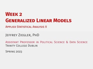
Download as PDF, PPTX


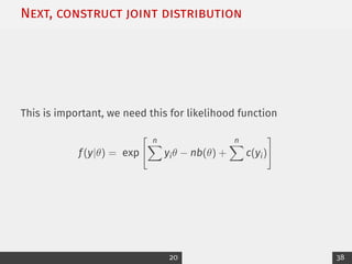
![Exponential Family: Canonical Form
The general expression is
f(y|θ) = exp[yθ − b(θ) + c(y)]
where
yθ multiplicative term have both y and θ
b(θ) ’normalising constant’
We want to isolate and derive b(θ)!
19 38](https://image.slidesharecdn.com/2glmsprintable-230323163124-0366f8e5/85/2_GLMs_printable-pdf-20-320.jpg)
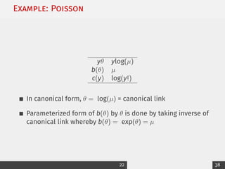
![Example: Poisson
f(y|µ) =
e−µµy
y!
= e−µ
µy
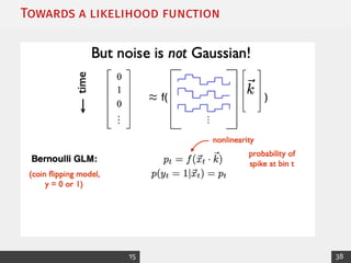
(y!)−1
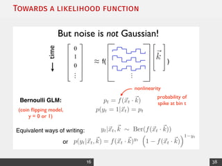
(1)
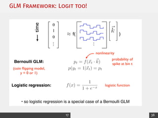
Let’s take log of expression, place it within an exp[]
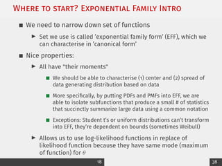
= exp [−µ + ylog(µ) − log(y!)]
= exp [ylog(µ) − µ − log(y!)]
(2)
where
yθ ylog(µ)
b(θ) µ
c(y) log(y!)
21 38](https://image.slidesharecdn.com/2glmsprintable-230323163124-0366f8e5/85/2_GLMs_printable-pdf-22-320.jpg)
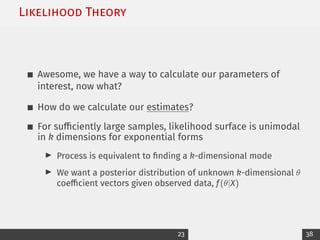
![Likelihood Theory
If θ̂ is estimate of θ that maximizes the likelihood function,
then L(θ̂|X) ≥ L(θ|X)∀θ ∈ Θ
To get expected value of y, E[y], we first need to differentiate
b(θ) with respect to θ whereby ∂
∂θ b(θ) = E[y]
We can follow these steps:
1. Take ∂
∂θ b(θ)
2. Insert canonical link function for θ
3. Obtain θ̂
26 38](https://image.slidesharecdn.com/2glmsprintable-230323163124-0366f8e5/85/2_GLMs_printable-pdf-27-320.jpg)
![Likelihood Theory
To get uncertainty estimate of θ̂ (its variance), we can take
the second derivative of b(θ) with respect to θ such that
∂2
∂θ2 b(θ) = E[(y − E[y])2]
We can then re-write the variance as1
1
a2(ψ)
var[y] → var[y] = a(ψ)
∂2
∂θ2
b(θ)
1
It’s useful to re-write canonical form to include a scale parameter, a(ψ). When a(ψ) = 1, then ∂2
∂θ2 b(θ) is
unaltered, (y|θ) = exp[
yθ−b(θ)
a(ψ)
+ c(y, ψ).
27 38](https://image.slidesharecdn.com/2glmsprintable-230323163124-0366f8e5/85/2_GLMs_printable-pdf-28-320.jpg)
![Likelihood Theory Ex: Poisson
We will also use canonical equation that includes a scale
parameter for Poisson
We know that inverse of canonical link gives us
b(θ) = exp[θ] = µ, which we will insert in
exp [ylog(µ) − µ − log(y!)] (3)
a(ψ)
∂2
∂θ2
b(θ) = 1
∂2
∂θ2
expθ|θ= log(µ)
= exp(log(µ))
θ̂ = µ
(4)
28 38](https://image.slidesharecdn.com/2glmsprintable-230323163124-0366f8e5/85/2_GLMs_printable-pdf-29-320.jpg)
![From parameter to estimate: Link Functions
We have essentially created a dependency connecting linear
predictor and θ (via µ in our Poisson example)
We can begin by making a generalization where V = Xβ + e
such that V represents a stocastic component, X denotes
model matrix, and β are estimated coefficients
We can then denote expected value as a linear structure,
E[V] = θ = Xβ
30 38](https://image.slidesharecdn.com/2glmsprintable-230323163124-0366f8e5/85/2_GLMs_printable-pdf-31-320.jpg)
![From parameter to estimate: Link Functions
Let’s now imagine that expected value of stocastic
component is some function, g(µ) that is invertible
Information from explanatory variables is now expressed
only through link (Xβ) to linear predictor, θ = g(µ), which is
controlled by link function, g()
We can then extend Generalized linear model to accomodate
non-normal response functions by transforming functions
linearly
This is achieved by taking inverse of link function, which
ensures Xβ̂ maintains linearity assumption required of
standard linear models
g−1
(g(µ)) = g−1
(θ) = g−1
(Xβ) = µ = E[Y]
31 38](https://image.slidesharecdn.com/2glmsprintable-230323163124-0366f8e5/85/2_GLMs_printable-pdf-32-320.jpg)


This document provides an overview of generalized linear models (GLMs) and maximum likelihood estimation (MLE). It discusses the exponential family distribution framework for GLMs, which allows the use of the same tools of inference across different distributions. It presents examples of link functions and canonical forms for the Gaussian and Poisson distributions. The document also covers likelihood theory and how to calculate parameter estimates and their uncertainty through taking derivatives of the log-likelihood function. It introduces MLE as a method for finding the parameter values that maximize the likelihood of observing the data. Computational estimation of GLMs is performed through an iterative least squares method using weights from the distributions' Fisher information.


