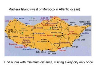
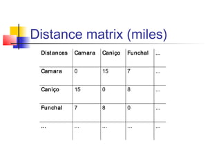
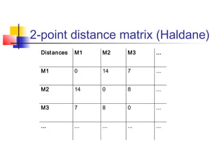
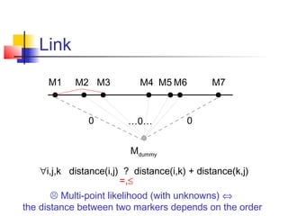
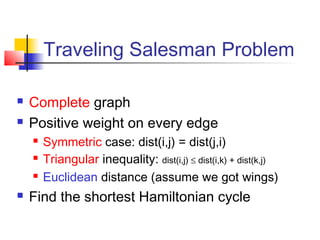
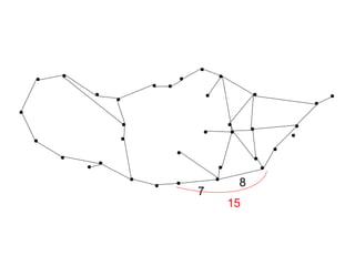
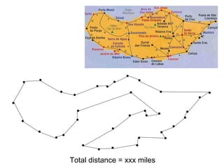
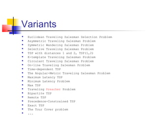
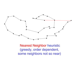
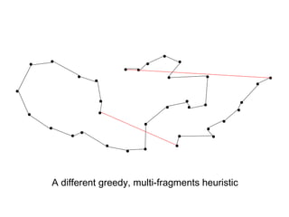
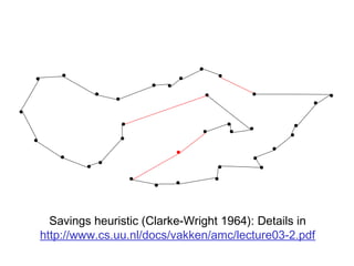
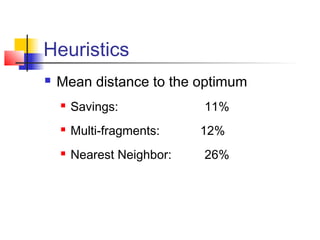
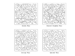
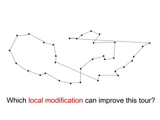
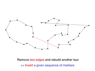
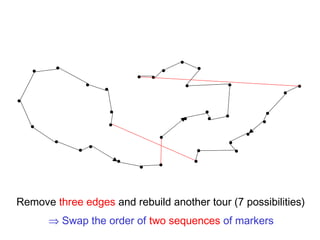
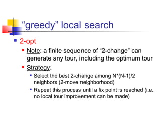
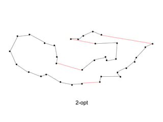
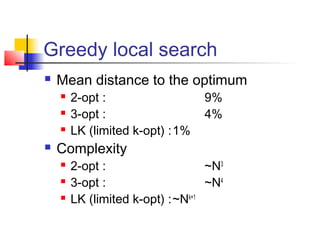
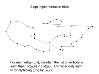
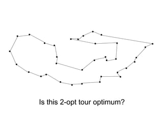
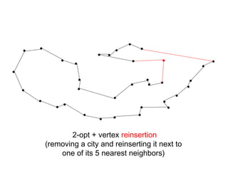
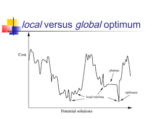
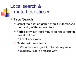
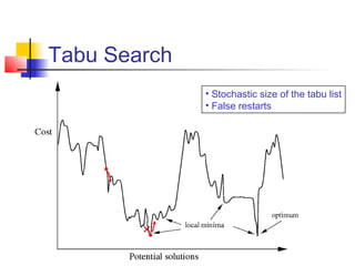
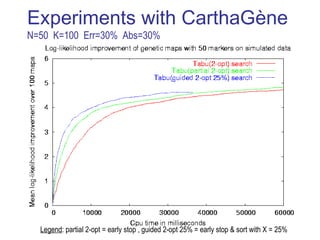
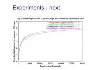
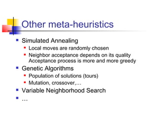
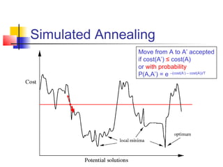
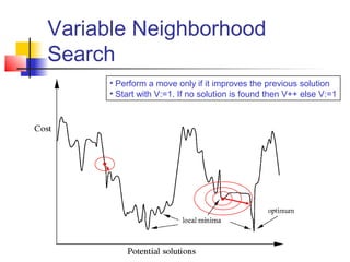
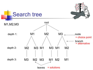
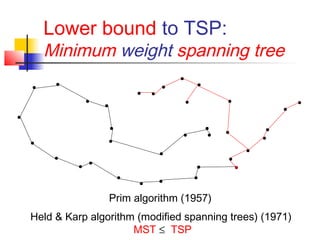
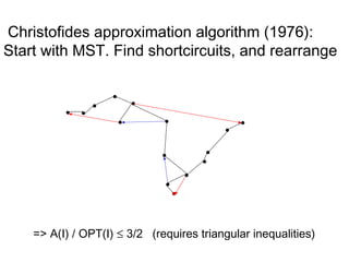
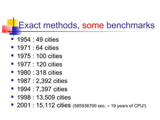
Carthagène
A brief introduction to combinatorial optimization:
The Traveling Salesman Problem
Simon de GivrySimon de Givry
Thales Research & Technology, FranceThales Research & Technology, France
(minor modifications by Benny Chor)
Find a tour with minimum distance, visiting every city only once
Madiera Island (west of Morocco in Atlantic ocean)
Distance matrix (miles)
Distances Camara Caniço Funchal ...
Camara 0 15 7 ...
Caniço 15 0 8 ...
Funchal 7 8 0 ...
... ... ... ... ...
Find an order of all the markers with maximum likelihood
A similar task in the genomic domain
2-point distance matrix (Haldane)
Distances M1 M2 M3 ...
M1 0 14 7 ...
M2 14 0 8 ...
M3 7 8 0 ...
... ... ... ... ...
Link
M1 M2 M3 M4 M5 M6 M7
Mdummy
0 0…0…
∀i,j,k distance(i,j) ? distance(i,k) + distance(k,j)
=,≤
 Multi-point likelihood (with unknowns) ⇔
the distance between two markers depends on the order
Traveling Salesman Problem
 Complete graph
 Positive weight on every edge
 Symmetric case: dist(i,j) = dist(j,i)
 Triangular inequality: dist(i,j) ≤ dist(i,k) + dist(k,j)
 Euclidean distance (assume we got wings)
 Find the shortest Hamiltonian cycle
7
8
15
Total distance = xxx miles
Traveling Salesman Problem
 Theoretical interest
 Basic NP-complete problem ( not easy)
 1993-2001: +150 articles about TSP in
INFORMS & Decision Sciences databases
 Practical interest
 Vehicle Routing Problem
 Genetic/Radiated Hybrid Mapping Problem

NCBI/Concorde, Carthagène, ...
Variants
 Euclidean Traveling Salesman Selection Problem
 Asymmetric Traveling Salesman Problem
 Symmetric Wandering Salesman Problem
 Selective Traveling Salesman Problem
 TSP with distances 1 and 2, TSP(1,2)
 K-template Traveling Salesman Problem
 Circulant Traveling Salesman Problem
 On-line Traveling Salesman Problem
 Time-dependent TSP
 The Angular-Metric Traveling Salesman Problem
 Maximum Latency TSP
 Minimum Latency Problem
 Max TSP
 Traveling Preacher Problem
 Bipartite TSP
 Remote TSP
 Precedence-Constrained TSP
 Exact TSP
 The Tour Cover problem
 ...
Plan
 Introduction to TSP
 Building a new tour “from scratch”
 Improving an existing tour
 Finding the best tour (or almost)
Building a new tour from scratch
Nearest Neighbor heuristic
(greedy, order dependent,
some neighbors not so near)
A different greedy, multi-fragments heuristic
Savings heuristic (Clarke-Wright 1964): Details in
http://www.cs.uu.nl/docs/vakken/amc/lecture03-2.pdf
Heuristics
 Mean distance to the optimum
 Savings: 11%
 Multi-fragments: 12%
 Nearest Neighbor: 26%
Improving an existing tour
Which local modification can improve this tour?
Remove two edges and rebuild another tour
⇔ Invert a given sequence of markers
Remove three edges and rebuild another tour (7 possibilities)
⇒ Swap the order of two sequences of markers
“greedy” local search
 2-opt
 Note: a finite sequence of “2-change” can
generate any tour, including the optimum tour
 Strategy:

Select the best 2-change among N*(N-1)/2
neighbors (2-move neighborhood)

Repeat this process until a fix point is reached (i.e.
no local tour improvement can be made)
2-opt
Greedy local search
 Mean distance to the optimum
 2-opt : 9%
 3-opt : 4%
 LK (limited k-opt) :1%
 Complexity
 2-opt : ~N3
 3-opt : ~N4
 LK (limited k-opt) :~Nk+1
Complexity n = number of vertices
Algorithm Complexity
A-TSP (n-1)!
S-TSP (n-1)! / 2
2-change 1
3-change 7
k-change (k-1)! . 2k-1
k-move (k-1)! . 2k-1
. n! / (k! . (n-k)!)
~ O( nk
) k << n
In practice: o( n )
2-opt et 3-opt ~ O( nk+1
)
In practice: o( n1.2
)
time(3-opt) ~ 3 x time(2-opt)
For each edge (u,v), maintain the list of vertices w
such that dist(w,v) < dist(u,v). Consider only such
w for replacing (u,v) by (w,v).
u
v
2-opt implementation trick:
Is this 2-opt tour optimum?
2-opt + vertex reinsertion
(removing a city and reinserting it next to
one of its 5 nearest neighbors)
local versus global optimum
Local search &
« meta-heuristics »
 Tabu Search
 Select the best neighbor even if it decreases
the quality of the current tour
 Forbid previous local moves during a certain
period of time

List of tabu moves
 Restart with new tours

When the search goes to a tour already seen

Build new tours in a random way
Tabu Search
• Stochastic size of the tabu list
• False restarts
Experiments with CarthaGène
N=50 K=100 Err=30% Abs=30%
Legend: partial 2-opt = early stop , guided 2-opt 25% = early stop & sort with X = 25%
Experiments - next
Other meta-heuristics
 Simulated Annealing
 Local moves are randomly chosen
 Neighbor acceptance depends on its quality
Acceptance process is more and more greedy
 Genetic Algorithms
 Population of solutions (tours)
 Mutation, crossover,…
 Variable Neighborhood Search
 …
Simulated Annealing
Move from A to A’ accepted
if cost(A’) ≤ cost(A)
or with probability
P(A,A’) = e –(cost(A’) – cost(A))/T
Variable Neighborhood
Search
• Perform a move only if it improves the previous solution
• Start with V:=1. If no solution is found then V++ else V:=1
Local Search
Demonstration
Finding the best tour
Search tree
M2M1 M3
M2 M3 M1 M3 M1 M2
M3 M2 M3 M1 M2 M1
M1,M2,M3
depth 1:
depth 2:
depth 3:
leaves
node
branch
root
= choice point
= alternative
= solutions
Tree search
 Complexity : n!/2 different orders
 Avoid symmetric orders (first half of the tree)
 Can use heuristics in choice points to order
possible alternatives
 Branch and bound algorithm
 Cut all the branches which cannot lead to a better
solution
 Possible to combine local search and tree
search
Lower bound to TSP:
Minimum weight spanning tree
Prim algorithm (1957)
Held & Karp algorithm (modified spanning trees) (1971)
MST ≤ TSP
Christofides approximation algorithm (1976):
Start with MST. Find shortcircuits, and rearrange
=> A(I) / OPT(I) ≤ 3/2 (requires triangular inequalities)
Exact methods, some benchmarks
 1954 : 49 cities
 1971 : 64 cities
 1975 : 100 cities
 1977 : 120 cities
 1980 : 318 cities
 1987 : 2,392 cities
 1994 : 7,397 cities
 1998 : 13,509 cities
 2001 : 15,112 cities (585936700 sec. ≈ 19 years of CPU!)

Helgaun's algorithm for the TSP

  • 1.
    Carthagène A brief introductionto combinatorial optimization: The Traveling Salesman Problem Simon de GivrySimon de Givry Thales Research & Technology, FranceThales Research & Technology, France (minor modifications by Benny Chor)
  • 2.
    Find a tourwith minimum distance, visiting every city only once Madiera Island (west of Morocco in Atlantic ocean)
  • 3.
    Distance matrix (miles) DistancesCamara Caniço Funchal ... Camara 0 15 7 ... Caniço 15 0 8 ... Funchal 7 8 0 ... ... ... ... ... ...
  • 4.
    Find an orderof all the markers with maximum likelihood A similar task in the genomic domain
  • 5.
    2-point distance matrix(Haldane) Distances M1 M2 M3 ... M1 0 14 7 ... M2 14 0 8 ... M3 7 8 0 ... ... ... ... ... ...
  • 6.
    Link M1 M2 M3M4 M5 M6 M7 Mdummy 0 0…0… ∀i,j,k distance(i,j) ? distance(i,k) + distance(k,j) =,≤  Multi-point likelihood (with unknowns) ⇔ the distance between two markers depends on the order
  • 7.
    Traveling Salesman Problem Complete graph  Positive weight on every edge  Symmetric case: dist(i,j) = dist(j,i)  Triangular inequality: dist(i,j) ≤ dist(i,k) + dist(k,j)  Euclidean distance (assume we got wings)  Find the shortest Hamiltonian cycle
  • 8.
  • 9.
  • 10.
    Traveling Salesman Problem Theoretical interest  Basic NP-complete problem ( not easy)  1993-2001: +150 articles about TSP in INFORMS & Decision Sciences databases  Practical interest  Vehicle Routing Problem  Genetic/Radiated Hybrid Mapping Problem  NCBI/Concorde, Carthagène, ...
  • 11.
    Variants  Euclidean TravelingSalesman Selection Problem  Asymmetric Traveling Salesman Problem  Symmetric Wandering Salesman Problem  Selective Traveling Salesman Problem  TSP with distances 1 and 2, TSP(1,2)  K-template Traveling Salesman Problem  Circulant Traveling Salesman Problem  On-line Traveling Salesman Problem  Time-dependent TSP  The Angular-Metric Traveling Salesman Problem  Maximum Latency TSP  Minimum Latency Problem  Max TSP  Traveling Preacher Problem  Bipartite TSP  Remote TSP  Precedence-Constrained TSP  Exact TSP  The Tour Cover problem  ...
  • 12.
    Plan  Introduction toTSP  Building a new tour “from scratch”  Improving an existing tour  Finding the best tour (or almost)
  • 13.
    Building a newtour from scratch
  • 15.
    Nearest Neighbor heuristic (greedy,order dependent, some neighbors not so near)
  • 16.
    A different greedy,multi-fragments heuristic
  • 17.
    Savings heuristic (Clarke-Wright1964): Details in http://www.cs.uu.nl/docs/vakken/amc/lecture03-2.pdf
  • 18.
    Heuristics  Mean distanceto the optimum  Savings: 11%  Multi-fragments: 12%  Nearest Neighbor: 26%
  • 20.
  • 21.
    Which local modificationcan improve this tour?
  • 22.
    Remove two edgesand rebuild another tour ⇔ Invert a given sequence of markers
  • 23.
    Remove three edgesand rebuild another tour (7 possibilities) ⇒ Swap the order of two sequences of markers
  • 24.
    “greedy” local search 2-opt  Note: a finite sequence of “2-change” can generate any tour, including the optimum tour  Strategy:  Select the best 2-change among N*(N-1)/2 neighbors (2-move neighborhood)  Repeat this process until a fix point is reached (i.e. no local tour improvement can be made)
  • 25.
  • 26.
    Greedy local search Mean distance to the optimum  2-opt : 9%  3-opt : 4%  LK (limited k-opt) :1%  Complexity  2-opt : ~N3  3-opt : ~N4  LK (limited k-opt) :~Nk+1
  • 27.
    Complexity n =number of vertices Algorithm Complexity A-TSP (n-1)! S-TSP (n-1)! / 2 2-change 1 3-change 7 k-change (k-1)! . 2k-1 k-move (k-1)! . 2k-1 . n! / (k! . (n-k)!) ~ O( nk ) k << n In practice: o( n ) 2-opt et 3-opt ~ O( nk+1 ) In practice: o( n1.2 ) time(3-opt) ~ 3 x time(2-opt)
  • 28.
    For each edge(u,v), maintain the list of vertices w such that dist(w,v) < dist(u,v). Consider only such w for replacing (u,v) by (w,v). u v 2-opt implementation trick:
  • 29.
    Is this 2-opttour optimum?
  • 30.
    2-opt + vertexreinsertion (removing a city and reinserting it next to one of its 5 nearest neighbors)
  • 31.
  • 32.
    Local search & « meta-heuristics » Tabu Search  Select the best neighbor even if it decreases the quality of the current tour  Forbid previous local moves during a certain period of time  List of tabu moves  Restart with new tours  When the search goes to a tour already seen  Build new tours in a random way
  • 33.
    Tabu Search • Stochasticsize of the tabu list • False restarts
  • 34.
    Experiments with CarthaGène N=50K=100 Err=30% Abs=30% Legend: partial 2-opt = early stop , guided 2-opt 25% = early stop & sort with X = 25%
  • 35.
  • 36.
    Other meta-heuristics  SimulatedAnnealing  Local moves are randomly chosen  Neighbor acceptance depends on its quality Acceptance process is more and more greedy  Genetic Algorithms  Population of solutions (tours)  Mutation, crossover,…  Variable Neighborhood Search  …
  • 37.
    Simulated Annealing Move fromA to A’ accepted if cost(A’) ≤ cost(A) or with probability P(A,A’) = e –(cost(A’) – cost(A))/T
  • 38.
    Variable Neighborhood Search • Performa move only if it improves the previous solution • Start with V:=1. If no solution is found then V++ else V:=1
  • 39.
  • 40.
  • 41.
    Search tree M2M1 M3 M2M3 M1 M3 M1 M2 M3 M2 M3 M1 M2 M1 M1,M2,M3 depth 1: depth 2: depth 3: leaves node branch root = choice point = alternative = solutions
  • 42.
    Tree search  Complexity: n!/2 different orders  Avoid symmetric orders (first half of the tree)  Can use heuristics in choice points to order possible alternatives  Branch and bound algorithm  Cut all the branches which cannot lead to a better solution  Possible to combine local search and tree search
  • 43.
    Lower bound toTSP: Minimum weight spanning tree Prim algorithm (1957) Held & Karp algorithm (modified spanning trees) (1971) MST ≤ TSP
  • 44.
    Christofides approximation algorithm(1976): Start with MST. Find shortcircuits, and rearrange => A(I) / OPT(I) ≤ 3/2 (requires triangular inequalities)
  • 45.
    Exact methods, somebenchmarks  1954 : 49 cities  1971 : 64 cities  1975 : 100 cities  1977 : 120 cities  1980 : 318 cities  1987 : 2,392 cities  1994 : 7,397 cities  1998 : 13,509 cities  2001 : 15,112 cities (585936700 sec. ≈ 19 years of CPU!)

Editor's Notes

  • #20 Savings : un sommet e1 est choisi comme le hub et on cree n-1 tours élémentaires e1-ei -e1. On fusionne (met bout a bout) en N-2 etapes deux sous tours e1-ei1-eik-e1 et e1-ej1-ejl-e1 en e1-ei1-eik-ej1-ejl-e1 tel que d(eik,1) + d(1,ej1) - d(eik,ej1) soit maximum