This document describes two algorithms for determining water depth from high-resolution satellite imagery: a standard linear transform algorithm and a new ratio transform algorithm. The linear transform requires tuning five parameters and does not work for very low albedo bottoms, while the ratio transform requires tuning only two parameters and can handle low albedo features. Both algorithms were tested on IKONOS imagery of two coral reef atolls in the Hawaiian Islands against lidar bathymetry data. The ratio transform performed as well as the linear transform and was more robust, stable between areas, and able to retrieve depths over 25m. However, it was also slightly noisier and had trouble resolving fine structures below 15-20m depth.

1. 547
Limnol. Oceanogr., 48(1, part 2), 2003, 547–556
᭧ 2003, by the American Society of Limnology and Oceanography, Inc.
Determination of water depth with high-resolution satellite imagery over variable
bottom types
Richard P. Stumpf1
and Kristine Holderied
NOAA National Ocean Service, Center for Coastal Monitoring and Assessment, 1305 East–West Highway rm 9115,
Silver Spring, Maryland 20910
Mark Sinclair
Tenix LADS Corporation, Mawson Park, South Australia, 5095, Australia
Abstract
A standard algorithm for determining depth in clear water from passive sensors exists; but it requires tuning of
five parameters and does not retrieve depths where the bottom has an extremely low albedo. To address these issues,
we developed an empirical solution using a ratio of reflectances that has only two tunable parameters and can be
applied to low-albedo features. The two algorithms—the standard linear transform and the new ratio transform—
were compared through analysis of IKONOS satellite imagery against lidar bathymetry. The coefficients for the
ratio algorithm were tuned manually to a few depths from a nautical chart, yet performed as well as the linear
algorithm tuned using multiple linear regression against the lidar. Both algorithms compensate for variable bottom
type and albedo (sand, pavement, algae, coral) and retrieve bathymetry in water depths of less than 10–15 m.
However, the linear transform does not distinguish depths Ͼ15 m and is more subject to variability across the
studied atolls. The ratio transform can, in clear water, retrieve depths in Ͼ25 m of water and shows greater stability
between different areas. It also performs slightly better in scattering turbidity than the linear transform. The ratio
algorithm is somewhat noisier and cannot always adequately resolve fine morphology (structures smaller than 4–5
pixels) in water depths Ͼ15–20 m. In general, the ratio transform is more robust than the linear transform.
Since the first use of aerial photography over clear shallow
water, it has been recognized that water depth can be esti-
mated in some way by remote sensing. The theory developed
by Lyzenga (1978, 1981) and expanded by Philpot (1989)
and Maritorena et al. (1994) demonstrated the validity of,
and problems involved with, using passive remote sensing
for determination of water depth. The use of two or more
bands allows separation of variations in depth from varia-
tions in bottom albedo, but compensation for turbidity, while
tractable, can be problematic. Although passive optical sys-
tems are limited in depth penetration and constrained by wa-
ter turbidity, the use of such satellite data might be the only
viable way to characterize either extensive or remote coral
reef environments. Besides the obvious need for bathymetric
information in many remote areas, mapping of coral reefs
and characterization of potential for bleaching requires in-
formation on water depth. Coral reefs, by their nature,
strongly influence the physical structure of their environ-
ment, and water depth information is fundamental to dis-
criminating and characterizing coral reef habitat, such as
patch reef, spur-and-groove, and seagrass beds. Knowledge
of water depth also allows estimation of bottom albedo,
which can improve habitat mapping (Mumby et al. 1998).
Knowledge of the detailed structure of the bottom helps in
1
Corresponding author (richard.stumpf@noaa.gov).
Acknowledgments
This effort was funded by the NOAA, National Ocean Service,
Coral Reef Mapping Program. Steve Rohmann provided overall co-
ordination of the Northwestern Hawaiian Islands project. The men-
tion of any company does not constitute an official endorsement by
NOAA.
characterizing the role and quality of the reef as a fish en-
vironment. However, extensive areas of coral reefs in the
ocean have little, incomplete, or spatially limited data on
bathymetry because of the difficulty obtaining accurate and
well-distributed soundings in remote reef areas. A robust
method of estimating bathymetry directly from the passive
satellite imagery would enhance our capability to map these
regions.
In order to map coral reef environments, high spatial res-
olution is required because of the relatively small horizontal
spatial scales and the ecological importance of vertical struc-
tures in those environments in the form of patch reefs, spur-
and-groove, mini-atolls, and so on. Mapping the fine-scale
variability will improve characterization of habitat, both for
corals and for various species living in the reefs. Until re-
cently, only two options existed for such information: air-
borne measurements (photo and hyperspectral) and multi-
spectral satellite imagery (typically Landsat). Although
aircraft can provide high-resolution data, either spatially or
spectrally, high costs and deployment issues limit their use
for comprehensive regional mapping in remote areas. Land-
sat, particularly the Landsat-7 enhanced thematic mapper
(ETM), offers global coverage of coral reefs, but only with
a 30-m field of view. With the launch of high-resolution
sensors IKONOS in 1999 and QuickBird in 2002, 4-m (or
better) field-of-view multispectral imagery became available
from space, providing a new resource for the development
of mapping and monitoring programs for coral reefs in re-
mote locations. These systems provide multispectral data
with three visible bands (blue, green, red), which can sim-
ulate aerial photography, and one near-infrared (near-IR)
band. This study focuses on IKONOS imagery; however, the

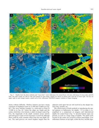
2. 548 Stumpf et al.
Table 1. Spectral bands for IKONOS, with Landsat-7 ETM for
comparison.
Spectral region
Spectral bands (nm)
IKONOS Landsat-7
Blue
Green
Red
Near-infrared
445–515
510–595
630–700
760–850
450–520
530–610
630–690
780–900
same depth estimation methods can be applied to Landsat
imagery because of the similarity in the spectral bands (Ta-
ble 1).
The standard bathymetry algorithm has a theoretical der-
ivation (Lyzenga 1978) but also incorporates empirical tun-
ing as an inherent part of the depth estimation process. It is
preferable to minimize such tuning, particularly for remote
regions where benthic and water quality parameters can be
hard to measure or estimate. This paper examines an alter-
native bathymetry algorithm and addresses two basic prob-
lems in the application of bathymetry algorithms to mapping
coral reefs: (1) the stability of an algorithm with fixed co-
efficients within and between atolls and (2) the behavior of
the algorithms in describing relative and absolute depths at
various scales.
Materials and methods
Study area—The area under investigation in this paper
includes two coral reef atolls in the northwest Hawaiian Is-
lands. This island chain extends over 1,800 km of the north
Pacific from Nihoa Island at 162ЊW to Kure Atoll at
178.5ЊW. The area encompasses two National Wildlife Ref-
uges, a Hawaiian State Wildlife Sanctuary, and the new U.S.
Northwestern Hawaiian Islands Coral Reef Ecosystem Re-
serve, which is proposed for designation as a U.S. National
Marine Sanctuary. There are 10 emergent atolls and reefs
and several shallow banks. The reef and bank areas include
Ͼ7,000 km2
of area less than 25 fathoms (45 m) in depth
(the absolute maximum depth detectable by passive remote
sensing and a boundary demarcation for some regulated ac-
tivities within the Reserve), making it the largest shallow-
water coral reef area under direct U.S. jurisdiction. The area
is remote, and the two atolls discussed here, Kure Atoll and
Pearl and Hermes Reef (henceforth called Pearl), are located
nearly 2,000 km from Honolulu. The shallow-water envi-
ronments of these two atolls are considerable in area, with
100 km2
at Kure and 500 km2
at Pearl. Kure Atoll was home
to a U.S. Coast Guard Loran station and has accurate sound-
ings within the lagoon, but few or no soundings in the fore-
reef area. In addition, outside of a narrow corridor to the
main island, many of the Kure reefs are not mapped in suf-
ficient detail to assure confidence in navigation. Even with
these limitations, Kure has more depth information than
Pearl, where one third of the lagoon has no bathymetric in-
formation at all, and the charts show only the general form
of the maze of mini-atolls and extensive lines of reticulated
reefs within the lagoon.
The atolls have substrates varying from sand to pavement
to live coral, with cover that includes various densities of
algae and smaller corals. The sand is usually coralline and
white with an extremely high albedo in higher energy areas.
With an increasing proportion of coral gravel and rubble, the
sediments tend to have a tan or brown appearance. Pavement
is typically gray to olive brown in appearance, varies from
low to high rugosity, and is often covered with varying den-
sities of algae. In areas where coral is found at high density
at Kure and Pearl, Porites compressa (finger coral) is the
most common species, with other dominant corals including
Montipora capitata (rice coral), Porites lobata (lobe coral),
Montipora flabellata (blue rice coral), and Pocillopora
meandrina (cauliflower coral). Algal cover includes varieties
of red, brown, and green macroalgae, as well as filamentous
turf algae. The reef flats are typically dominated by encrust-
ing coralline algae, with some green algae (e.g., Halimeda
sp.).
Model—The depth estimation method uses the reflectanc-
es for each satellite imagery band, calculated with the sensor
calibration files and corrected for atmospheric effects. The
reflectance of the water, Rw, which includes the bottom
where the water is optically shallow, is defined as
␲L (␭)w
R ϭ (1)w
E (␭)d
where Lw is the water-leaving radiance, Ed is the downwell-
ing irradiance entering the water, and ␭ is the spectral band.
Lw and Rw refer to values above the water surface. Rw is
found by correcting the total reflectance RT for the aerosol
and surface reflectance, as estimated by the near-IR band,
and for the Rayleigh reflectance Rr (Eq. 2).
Rw ϭ RT(␭i) Ϫ Y(␭i)RT(␭IR) Ϫ Rr(␭i) (2)
Y is the constant to correct for spectral variation (equivalent
to the Angstrom exponent in Gordon et al. [1983]), subscript
i denotes a visible channel, and subscript IR denotes the
near-IR channel. RT is found from Eq. 3.
␲L (␭ )/E (␭ )T i 0 i
R (␭ ) ϭ (3)T i 2
(1/r )T (␭ )T (␭ )cos ␪0 i 1 i 0
LT is the (total) radiance measured at the satellite, E0 is the
solar constant, r is the earth–sun distance in astronomical
units, ␪0 is the solar zenith angle, and T0 and T1 are the
transmission coefficients for sun-to-earth and earth-to-satel-
lite, respectively.
The atmospheric correction is based on the algorithm de-
veloped by Gordon et al. (1983) for the Coastal Zone Color
Scanner (CZCS) and by Stumpf and Pennock (1989) for the
Advanced Very High Resolution Radiometer (AVHRR) and
is similar to that recommended for Landsat (Chavez 1996;
Zhang et al. 1999). The Y coefficient in Eq. 2 depends on
aerosol type. For IKONOS, the correction presumes a mar-
itime atmosphere with a spectral variation similar to that of
the water surface specular reflectance. This proves to be a
reasonable assumption here; however, separation of the aero-
sol correction (with a scale of hundreds of meters) from the
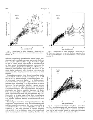
specular surface reflectance correction (with a scale of tens

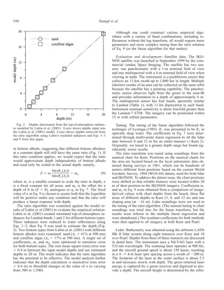
3. 549Satellite-derived water depth
Fig. 1. Log transformation used for ratio algorithm with data
from Kure Atoll. The lines of constant depth are also lines of fixed
ratio (0.3 m is also the blue to green ratio of 0.975; 18 m is a ratio
of 1.251). Depths were assigned to the constant ratio lines using the
tuning described in this paper. The dashed line shows the approxi-
mate values for a sand bottom that has the same albedo at all depths.
The attenuation of light with depth means that features have lower
Rw in deeper water, regardless of their intrinsic albedo. A decrease
in albedo causes values to move down the lines of constant ratio.
‘‘High Ad’’ indicates carbonate sand of nominally similar albedo at
both 0.3 and 18 m. ‘‘Low Ad’’ indicates similar albedo over dense
algal cover at both depths.
of meters) might be required for more generic use of IKO-
NOS data. Although IKONOS does not have onboard cali-
bration, postlaunch calibrations have been established by the
commercial vendor, Space Imaging. Additional comparisons
with Landsat-7, which does have onboard calibration, as well
as the sea-viewing wide field-of-view sensor (SeaWiFS),
might aid in calibration for future work. Residual miscali-
bration will result in alteration of the atmospheric model of
choice and, to a lesser degree, in the empirical coefficients
chosen for the depth estimation algorithms.
Bathymetry—Linear transform: Light is attenuated expo-
nentially with depth in the water column, with the change
expressed by Beer’s Law (Eq. 4).
L(z) ϭ L(0)exp(ϪKz) (4)
K is the attenuation coefficient and z is the depth. Any anal-
ysis of light with depth must take into account this expo-
nential decrease in radiance with depth. Lyzenga (1978)
showed that the relationship of observed reflectance (or ra-
diance) to depth and bottom albedo could be described as
Rw ϭ (Ad Ϫ Rϱ)exp(Ϫgz) ϩ Rϱ (5)
where Rϱ is the water column reflectance if the water were
optically deep, Ad is the bottom albedo, z is the depth, and
g is a function of the diffuse attenuation coefficients for both
downwelling and upwelling light. Equation 5 can be rear-
ranged to describe the depth in terms of the reflectances and
the albedo (Eq. 6).
z ϭ gϪ1
[ln(Ad Ϫ Rϱ) Ϫ ln(Rw Ϫ Rϱ)] (6)
The estimation of depth from a single band using Eq. 6
will depend on the albedo Ad, with a decrease in albedo
resulting in an increase in the estimated depth. Lyzenga
(1978, 1985) showed that two bands could provide a cor-
rection for albedo in finding the depth and created from Eq.
6 the linear solution in Eq. 7.
Z ϭ a0 ϩ aiXi ϩ ajXj (7)
where
Xi ϭ ln[Rw(␭i) Ϫ Rϱ(␭i)] (8)
The constants a0, ai, and aj usually are determined from mul-
tiple linear regression (or a similar technique). For any so-
lution for depth from passive systems, variations in water
clarity and spectral variation in absorption pose additional
complications (Philpot 1989; Van Hengel and Spitzer 1991).
The linear transform solution above has five variables that
must be determined empirically: Rϱ(␭i), Rϱ(␭j), a0, ai, and aj.
Having to adjust five empirical coefficients can be problem-
atic for large areas, even with relatively small variations in
water quality conditions. In addition, when the bottom al-
bedo is low, as can occur with dense macroalgae or seagrass,
then Ad is less than Rϱ. As a result, the depth cannot be found
without using an entirely new algorithm, because X is un-
defined if (Rw Ϫ Rϱ) is negative (logarithm of a negative
number).
Ratio transform: The problem of mapping shallow-water
areas with significantly lower reflectance than adjacent, op-
tically deep waters provided the initial motivation to develop
an alternative algorithm. Because we are interested in map-
ping relatively large and remote coral reef areas, we also
searched for an alternative solution that has fewer parame-
ters, thereby requiring less empirical tuning and having the
potential of being more robust over variable bottom habitats.
With bands having different water absorptions, one band
will have arithmetically lesser values than the other. Ac-
cordingly, as the log values change with depth, the ratio will
change (Fig. 1). As the depth increases, while the reflectance
of both bands decreases, ln(Rw) of the band with higher ab-
sorption (green) will decrease proportionately faster than
ln(Rw) of the band with lower absorption (blue). According-
ly, the ratio of the blue to the green will increase. A ratio
transform will also compensate implicitly for variable bot-
tom type. A change in bottom albedo affects both bands
similarly (cf. Philpot 1989), but changes in depth affect the
high absorption band more. Accordingly, the change in ratio
because of depth is much greater than that caused by change

4. 550 Stumpf et al.
Fig. 2. Depths determined from the top-of-atmosphere radianc-
es modeled by Lubin et al. (2001). X-axis shows depths input into
the Lubin et al. (2001) model. Y-axis shows depths retrieved from
the ratio algorithm using Lubin’s modeled radiances and Eqs. 1–3
and 9 from this paper.
in bottom albedo, suggesting that different bottom albedoes
at a constant depth will still have the same ratio (Fig. 1). If
this ratio condition applies, we would expect that the ratio
would approximate depth independently of bottom albedo
and need only be scaled to the actual depth; namely,
ln(nR (␭ ))w i
Z ϭ m Ϫ m (9)1 0
ln(nR (␭ ))w j
where m1 is a tunable constant to scale the ratio to depth, n
is a fixed constant for all areas, and m0 is the offset for a
depth of 0 m (Z ϭ 0), analogous to a0 in Eq. 7. The fixed
value of n in Eq. 9 is chosen to assure both that the logarithm
will be positive under any condition and that the ratio will
produce a linear response with depth.
The ratio algorithm was examined against the model re-
sults of Lubin et al (2001) to evaluate the empirical solution.
Lubin et al. (2001) created simulated top-of-atmosphere ra-
diances for Landsat bands 1 and 2 for different bottom types.
These radiances were reduced to water reflectances using
Eqs. 1–3, then Eq. 9 was used to estimate the depth (Fig.
2). Two bottom types from Lubin et al. (2001) with different
bottom albedos were examined: sand (Ad ϭ 41% at 500 nm)
and coralline algae (Ad ϭ 17% at 500 nm). A single set of
coefficients, m1 and m0, were optimized to minimize error
for both bottom types. The root mean square (rms) error was
Ͻ 0.4 m between the input model depths and our estimated
depths to 20 m. The result indicates that the ratio algorithm
has the potential to be effective. The model analysis further
indicates that the depth calculation is insensitive (rms error
Ͻ 0.4 m) to threefold changes in the value of n (n varying
from 500 to 1,500).
Although one could construct various empirical algo-
rithms with a variety of band combinations, including re-
flectances without the log transform, all would require more
parameters and more complex tuning than the ratio solution
of Eq. 9 (or the linear algorithm for that matter).
Evaluation and development—Satellite data: The IKO-
NOS satellite was launched in September 1999 by the com-
mercial vendor, Space Imaging. The satellite has two sen-
sors: one panchromatic with a 1-m nominal field of view
and one multispectral with a 4-m nominal field of view when
viewing at nadir. The instrument is a pushbroom sensor that
collects an 11-km swath up to 1,000 km in length. Multiple
(shorter) swaths of an area can be collected on the same orbit
because the satellite has a pointing capability. The panchro-
matic sensor observes light from the green to the near-IR
and provides information to a depth of approximately 6 m.
The multispectral sensor has four bands, spectrally similar
to Landsat (Table 1), with 11-bit digitization in each band.
Instrument nominal sensitivity is about fourfold greater than
the Landsat-7 ETM. The imagery can be positioned within
15 m with orbital parameters.
Tuning: The tuning of the linear algorithm followed the
technique of Lyzenga (1985). Rϱ was presumed to be Rw in
optically deep water. The coefficients in Eq. 7 were deter-
mined through multivariate linear regression to all the lidar
data between 0 and 12 m for an entire transect (ϭKure 2).
Originally, we tuned to a greater depth range but found sig-
nificantly worse results.
The ratio transform was tuned using soundings from the
nautical chart for Kure. Positions on the nautical charts for
the area are located based on the local astronomic data ob-
tained during surveys in 1961, which can be hundreds of
meters different from positions based on the current World
Geodetic Survey, 1984 (WGS-84) datum, used for both lidar
and IKONOS. To address the datum issue, the chart positions
were shifted so that reliable features were located within 20
m of their position in the IKONOS imagery. Coefficients m1
and m0 in Eq. 9 were obtained from a comparison of image-
derived values with chart depths from the beach, three flat
areas of different depths in Kure (3, 8, and 12 m) and one
sloping area (at ϳ16 m). Lidar soundings were not used in
the tuning of the ratio algorithm. (The manual tuning to chart
soundings was tried also for the linear transform, but the
results were inferior to the multiple linear regression and
were abandoned.) The resultant coefficients for both methods
were then applied to all imagery at both Kure and Pearl.
Lidar: Bathymetry was obtained using the airborne LADS
Mk II lidar system along eight transects over Kure and 10
over Pearl. Depths from three of these transects are discussed
in detail here. The instrument uses a Nd-YAG laser with a
532-nm wavelength. The scanning laser operates at 900 Hz,
and the aircraft ground speed is about 150 knots, resulting
in a 4- ϫ 4-m laser spot spacing across a swath of ϳ200 m.
The footprint of the laser at the water surface is about 2.5
m and increases slowly with depth. The green returned laser
energy is captured by a green receiver and digitized to pro-
vide a depth. The aircraft height is determined by the infra-

5. 551Satellite-derived water depth
Fig. 3. Profile from Kure Atoll (Kure 2 in text). Distances are
in meters from start of lidar line in southwest. Soundings from the
nautical chart used for tuning were located in the vicinity of dis-
tances 9,000, 3,000, 6,000, and 1,500 m. The depth discrepancy at
1,000 m occurred in a light cloud shadow and should be disregard-
ed; the ratio method does not necessarily perform better under cloud
shadows than the linear method.
Fig. 4. Profile across forereef (on either side), reef crest, and
back reef at Kure Atoll (Kure 1 in text). Depth discrepancies be-
tween 1,800 and 2,000 m occur in light cloud shadow.
Fig. 5. Profile from Pearl and Hermes Atoll (Pearl 1 in text),
crossing patch reefs, mini-atolls, and reef-crest (at 16,000 m).
red laser reflection, which is supplemented by an inertial
height reference. The aircraft position was based on Global
Positioning System (GPS) measurements by postprocessing
against an Ashtech GPS station located at a known reference
on Midway Island. Total expected error for horizontal po-
sition of a laser sounding was 4 m for this mission. Position
of the bottom was determined in an absolute sense against
the WGS-84 ellipsoid used for positioning, and the bathym-
etry was determined by comparing returns from the water
surface and the bottom. The maximum water penetration
(where a return was reported) in the clearest water in this
area exceeded 60 m. The survey met International Hydro-
graphic Standards for accuracy of order 1. Vertical precision
of measured relative water depth was Ͻ5 cm, as indicated
by the crossline comparisons. To determine height relative
to mean lower low water, the standard datum for bathymetry,
a tidal correction for Midway Island was applied (80 km
from Kure and 130 km from Pearl) because tide gauges were
not present at either Kure or Pearl. Residual errors from tide
uncertainty can be expected to be Ͻ15 cm, which is finer
than the 30-cm vertical resolution achievable with satellite
detection.
Results
The algorithms were examined along three lidar lines; the
first of which is an 11-km transect extending across Kure
(ϭKure 2) from the southwest, a forereef area through the
central lagoon to the northeast reef crest, and the forereef
(Fig. 3). The central basins were slightly turbid with fine
suspended sediment; however the density of this turbidity
was insufficient to alter the brightness of the red band, and
visibility was typically over 10 m, even in the more turbid
areas. A second Kure lidar transect (ϭKure 1) of 6 km ex-
tends across the northern portion of the atoll from west to
east, covering only the forereef and shallow areas along the
backreef (Fig. 4). The third transect examined here is a 17-
km line running south to north across Pearl (ϭPearl 1) and
crossing many steep, reticulated reef structures (Fig. 5). The
coefficients tuned to the Kure 2 transect were applied di-
rectly to IKONOS imagery from Pearl, without retuning for
either the ratio or linear algorithms.
The bathymetry generated by both algorithms is generally
effective in mapping depths across both Kure and Pearl, de-
spite distinct differences in the structure of the two atolls,
with Kure having a classic atoll lagoon and Pearl having an
extensive and complicated reef structure within the lagoon
(Fig. 5). Most major vertical features are reproduced (Fig.
6), particularly in shallow water, including shallow basins
with sand waves, spur-and-groove on the forereef (Fig. 6A),
patch reefs (Fig. 6B), and steep, narrow reticulated reef
structures (Fig. 6C,D). Spatial details are also well repre-
sented, as can be seen in Fig. 7, which shows an area of
Kure with patch reefs in deeper water and sand waves in
shallow water. Along the two Kure transects, depths gener-
ated with both methods match the lidar data in water less
than ϳ15 m depth. The results from Pearl illustrate a general
transferability of the algorithms (Fig. 5), since both methods
give meaningful results (to ϳ15 m) without retuning. Both
algorithms also quite effectively recover the steep depth var-
iability over the complex mini-atolls and reticulated reefs of
Pearl, including the small depth increase characteristic of the
normally sandy center of mini-atolls. However, in relatively

6. 552 Stumpf et al.
Fig. 6. Detailed profiles of depth (meters) and blue reflectance, Rw(blue). Tick marks on all
graphs mark 100-m distance. (A) Kure 1: profile over spur-and-groove type structure on forereef.
(B) Kure 2: profile over algae-covered pavement (former patch reefs). (C) Pearl 1: profile over
coral-dominated patch and reticulated reefs. (D) Pearl 1: profile over mix of sand- and coral-dom-
inated reefs. Note that several of the shallow areas have lower reflectance (e.g., centered near 5,700
and 6,300 m in panel D) and that the centers of the vertical reef structures at 12,300 and 13,600
m in panel C have a narrow area of low reflectance.
high-turbidity water in the basins in the southeast of the
lagoon (e.g., 5,500 m in Fig. 6D), these passive methods
fail, in that the true bottom cannot be detected in Ͼ15 m of
water, and both algorithms generate a false bottom. This fail-
ure illustrates a fundamental limitation of depth estimation
from optical systems, regardless of method.
The effectiveness of both algorithms in resolving bathy-
metric variations independently of variations in bottom al-
bedo is demonstrated in several areas. Shallow structures
with algae and pavement are tightly resolved (Fig. 6B), and
patch reefs and mini-atolls are resolved even with dramatic
variations in reflectance (Fig. 6C,D) between the dark, shal-
low reefs and the light, typically sandy-bottom, deep basins
(Fig. 7). Reef cover varies from algae-covered pavement to
dense Porites colonies, introducing two- to fourfold varia-
tion in Rw(blue); yet, the algorithms resolve the depth vari-

7. 553Satellite-derived water depth
Fig. 7. Depths from the three methods and ‘‘true-color’’ water reflectance for central Kure: (A) ratio, (B) linear, (C) true-color, and (D)
lidar. The lidar swaths are 200 m wide and marked on each image. Depths are shown in meters with scale bar at lower right. The box (at
upper right in each image) marks a patch reef of low reflectance. IKONOS imagery courtesy of Space Imaging.
ations without difficulty. Shallow features can have strong
variations in brightness (seen at 12,300 and 13,600 m in Fig.
6C). The most striking example is a mini-atoll in Pearl at
13,600 m in Fig. 6C, where the edges are bright and the
center, which has a live bottom, is dark. In deeper water (Fig.
6A), the magnitude of the depth variation across narrow
spur-and-groove types of reef structures is resolved, although
there could be some constant offset from the true depth val-
ues. The sand grooves are much brighter targets than the
adjacent coral spurs but are still resolved as the deeper fea-
tures they actually are.
The effectiveness of both methods in reproducing the spa-
tial patterns in bathymetry for depths Ͻ12 m deep is ex-
emplified in a comparison of imagery and lidar-derived
depths for central Kure (Fig. 7). Several bottom types are
present, as well as a large range of depths. The patch reefs
located in the center are covered in dense macroalgae. Low
reflectance features at top right, within the box, include alga-

8. 554 Stumpf et al.
Fig. 8. Comparison of all depths along Kure 1 (those from Fig.
4). The discrepancy in depth at 5 m occurred under a cloud shadow
(see Fig. 4).
Fig. 9. Comparison of all depths along Kure 2 (those from Fig.
3). The severe discrepancy in depth in the linear algorithm from
25–30 m (derived depths Ͻ 10 m) occurred under a cloud shadow
(see Fig. 3).
Fig. 10. Comparison of all depths along Pearl 1 (those from
Fig. 5). A difference between clear and turbid areas is indicated.
Areas of clear water on the forereef show consistent retrievals to
20 m with the ratio algorithm. Areas in the turbid zone of the lagoon
have underestimated depths with few retrievals Ͼ15 m.
and coral-covered reefs. Elsewhere the bottom is sand, tran-
sitioning to a lower albedo carbonate pavement in the lower
left. Along the right side of the image, the shallow depths
are part of a large, bright, sandy region on the east side of
the Kure lagoon. Both methods pick up the transition to the
shallower depths, despite the much brighter reflectances, al-
though the linear method tends to bias low relative to the
actual depths. Sand waves in 2.5–4-m-deep water across the
eastern side of the Kure lagoon were also resolved by both
methods.
Scatterplot comparisons of the derived versus lidar depths
show that both methods reproduce the depths up to 10–15
m (Figs. 8–10), with best results for the tuned transect (Fig.
9), as expected. However in depths Ͼ15 m, the linear trans-
form rarely retrieves meaningful depths. The ratio transform
provides depth information 5–10 m deeper than the linear
transform. The ratio transform does have a greater amount
of noise, which is not surprising since a ratio combination
will inherently amplify small differences more than a linear
combination and the error variability increases with depth.
In the deep (lidar depths Ͼ 20 m) turbid basins of Pearl, the
linear transform failed before the ratio transform (Fig. 10).
Conversely, in the clear water of the deep forereef along
Kure 1 (Fig. 8), depth retrievals are possible to nearly 30 m
with the ratio algorithm, whereas the linear transform fails
at 12–15 m.
Examining the normalized error against depth shows the
difference in the effectiveness of the two methods with depth
and between different transects. The ratio transform has a
consistent normalized rms error of Ͻ0.3 (30%) in Ͻ25 m of
water (Fig. 11). The linear transform, as expected, performs
well up to 10–15 m, but the failure at that point is manifested
in the increasing rms error. It is surprising that the ratio

9. 555Satellite-derived water depth
Fig. 11. Normalized root mean square (rms) error (ratio of rms
error to actual depth) in 2.5-m bins for (A) Kure 1, (B) Kure 2, and
(C) Pearl. The bin at 2.5 m depth was dropped because the nor-
malization was problematic for both algorithms with water Յ0.6 m.
transform performed as well as the linear transform along
Kure 2 in waters Ͻ15 m depth because the linear transform
was tuned to the very lidar data being used for the error
evaluation, whereas the ratio transform was tuned to only a
few, independent nautical chart soundings. To investigate the
stability of tuning methods, the linear transform was tuned
to lidar for the Kure 1 transect. This tuning produced poor
results, with normalized rms errors Ͼ0.5 when applied to
Kure 2.
Discussion
The ratio transform method addresses several issues that
have considerable relevance to using passive multispectral
imagery to map shallow-water bathymetry. First, it does not
require subtraction of dark water, which expands the number
of benthic habitats over which it can be applied. Second, the
ratio transform method has fewer empirical coefficients re-
quired for the solution, which makes the method easier to
use and more stable over broader geographic areas. Third,
the ratio method can be tuned using available (reliable)
soundings. And finally, the results shown here demonstrate
that the ratio method has superior depth penetration to the
linear method for a Pacific Ocean region with relatively clear
water. The ratio transform has limitations relative to the lin-
ear transform, particularly in an increased level of noise.
Our first use of IKONOS imagery (Baker Island in the
central Pacific) showed shallow-water areas that had lower
reflectance than deep water, so the linear transform could not
be implemented. Although Kure and Pearl do not have shal-
low-water areas that are less reflective than deep water (typ-
ically caused by extremely dense algae or seagrass cover),
we have found patches of algae of Ն1 km2
within the north-
western Hawaiian island chain that have a reflectance darker
than deep water. Solutions for the linear transform to solve
the low-albedo issue have been proposed (Van Hengel and
Spitzer 1991) but require tuning of the patch as well, which
only increases the number of required coefficients. The stan-
dard linear method requires five coefficients that vary with
environmental conditions: Rϱ(␭i), Rϱ(␭j), a0, ai, and aj, where-
as the ratio method requires only two: m0 and m1. As a result,
the ratio solution is simple to execute, since tuning can be
achieved with a handful of accurate soundings. This is not
a trivial issue when working in areas where few soundings
are available.
The determination of Rϱ probably introduces more uncer-
tainty in the linear algorithm than any other coefficient. With
any variation in scattering, Rϱ will change in both bands,
and with variations in absorption, Rϱ will change in the blue
band. This is extremely difficult to determine locally and can
easily vary throughout a scene. Failure to correctly deter-
mine Rϱ will affect the depth determination for deeper water.
New optimization methods that have been proposed for hy-
perspectral instrumentation might resolve this by solving for
Rϱ (Lee et al. 1999). Such methods could be useful for geo-
graphically large mapping projects when hyperspectral im-
agery becomes routinely available with standard processing.
The ratio transform requires only bands with different water
absorption and so might be applied to any sensor detecting
the appropriate wavelengths.
In addition to applying the ratio transform method to more
Pacific Ocean atolls, we plan to investigate ways of improv-
ing the current algorithm, in particular to examine methods
for addressing moderate turbidity. The linear algorithm has
an inherent solution for albedo, which must also be exam-
ined for the ratio algorithm. The simple tuning, stable results,
and superior depth penetration argue for application of the
ratio algorithm for mapping water depths in extensive coral
reef environments similar to those found in this study.
References
CHAVEZ, P. S. 1996. Image-based atmospheric corrections—revis-
ited and improved. Photogramm. Eng. Remote Sens. 62: 1025–
1035.
GORDON, H. R., D. K. CLARK, J. W. BROWN, O. B. BROWN, R. H.
EVANS, AND W. W. BROENKOW. 1983. Phytoplankton pigment

10. 556 Stumpf et al.
concentrations in the Middle Atlantic Bight: Comparison of
ship determinations and CZCS estimates. Appl. Opt. 22: 20–
36.
LEE, Z., K. L. CARDER, C. D. MOBLEY, R. G. STEWARD, AND J. S.
PATCH. 1999. Hyperspectral remote sensing for shallow waters:
2. Deriving bottom depths and water properties by optimiza-
tion. Appl. Opt. 38: 3831–3843.
LUBIN, D., W. LI, P. DUSTAN, C. MAXEL, AND K. STAMNES. 2001.
Spectral signatures of coral reefs: Features from space. Remote
Sens. Environ. 75: 127–137.
LYZENGA, D. R. 1978. Passive remote sensing techniques for map-
ping water depth and bottom features. Appl. Opt. 17: 379–383.
. 1981. Remote sensing of bottom reflectance and water at-
tenuation parameters in shallow water using aircraft and Land-
sat data. Int. J. Remote Sens. 1: 71–82.
. 1985. Shallow-water bathymetry using combined lidar and
passive multispectral scanner data. Int. J. Remote Sens. 6: 115–
125.
MARITORENA, S., A. MOREL, AND B. GENTILI. 1994. Diffuse reflec-
tance of oceanic shallow waters: Influence of water depth and
bottom albedo. Limnol. Oceanogr. 39: 1689–1703.
MUMBY, P. J., C. D. CLARK, E. P. GREEN, AND A. J. EDWARDS.
1998. Benefits of water column correction and contextual ed-
iting for mapping coral reefs. Int. J. Remote Sens. 19: 203–
210.
PHILPOT, W. D. 1989. Bathymetric mapping with passive multi-
spectral imagery. Appl. Opt. 28: 1569–1578.
STUMPF, R. P., AND J. R. PENNOCK. 1989. Calibration of a general
optical equation for remote sensing of suspended sediments in
a moderately turbid estuary, J. Geophys. Res. Oceans 94:
14,363–14,371.
VAN HENGEL, W., AND D. SPITZER. 1991. Multi-temporal water
depth mapping by means of Landsat TM. Int. J. Remote Sens.
12: 703–712.
ZHANG, M., K. CARDER, F. E. MULLER-KARGER, Z. LEE, AND D. B.
GOLDGOF. 1999. Noise reduction and atmospheric correction
for coastal applications of landsat thematic mapper imagery.
Remote Sens. Environ. 70: 167–180.
Received: 17 October 2001
Accepted: 8 July 2002
Amended: 29 August 2002