1. Introduction
Field Area
Obtaining Ground Truth Measurements
Coupling
Coupling was a major challenge in the
lower-lying area. The area was very spongy
with wet moss. Despite driving the
geophones approximately 0.33-m below the
surface, we recorded poor quality data. For
the 0.33-m spacing array, we improved
coupling by digging a small hole, filling the
hole with sand and then inserting the
geophone into the sand. The two surveys in
this environment took two days.
Challenges
• HVSR shows promise for tracking active-layer changes in
permafrost.
• HVSR would enable remote tracking of depth to contrasting
layer with existing stations.
• Potential to use historical data to see long-term trends
• Quarter-wavelength approximation are successful in
reproducing a small fraction of the high-frequency spectra
• Future work will focus on HVSR inversions using the
technique of Herak, 2008.
Summary
Seasonal changes in H/V spectral ratio at high-latitude
seismic stations
Rebekah F. Lee, Robert E. Abbott, Hunter A. Knox, Aasha Pancha
1. NC State University, Raleigh North Carolina 2. Sandia National Labs, Albuquerque New Mexico 3. Victoria University, Wellington New Zealand
Sandia National Laboratories is a multi-program laboratory managed and operated by Sandia Corporation, a wholly owned subsidiary of Lockheed Martin Corporation, for the U.S. Department of Energy’s National Nuclear Security Administration under contract DE-AC04-94AL85000.
Using the 8 lb
hammer for the
ReMi survey
We show results for
three of six stations:
R1B, CE1 and R2C
Possible layers at
site
m
• We used two methods to find depth-to-frozen-ground
• Method 1: Physical probing of the ground with a metal rod
• Method 2: Refraction-Microtremor active-source seismic
method.
Thickness measurements
In most locations, the interface between
thawed (active layer) and frozen
permafrost layers was obvious. In some
places, the rod could be pushed further in
the ground but with higher resistance. This
occurred in some areas where the depth
measurements were over 1 meter. We
believe this was because of degraded, or
partially frozen, permafrost. Identifying the
transition from thawed to partially frozen
soil was difficult. Reliable measurements
with this boundary would be helpful if
possible in the future.
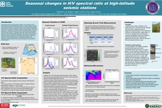
Seasonal Variation in HVSR
Frozen Ground Partially Thawed Ground
• Stations CE1 and R1B show seasonal peaks in HVSR. Station
R2C shows pronounced peaks year-round. R2C is the only station
located in forested (Black Spruce) area.
• During the winter months the ground is frozen to the surface and
stations exhibit flat spectral ratios above 6 Hz. As the ground thaws
from the surface downward there is much more variation at higher
frequencies. As expected, lower frequencies representing greater
active-layer depths are consistent year-round.
• Peak at 2.5 Hz is consistent year-round and represents deeper
structure, most likely depth to basement rock.
•Using the quarter-wavelength approximation with h= 45 cm (June
ground truth, next column), and Vs = 100 m/s (Holzer et. al, 2005;
mud Vs) results in a peak at 55 Hz. This agrees nicely with the high
frequency secondary peak. This peak migrates to 35 Hz, where a
small shoulder is seen, for 68 cm depth (October ground truth).
•The main peaks remain unexplained. Future work will use the
methods of Herak (2008) for a full HVSR inversion.
Analysis
We present results demonstrating seasonal variations in the Horizontal-to-Vertical
Spectral Ratio (HVSR) at high-latitude seismic stations. We analyze data from a site at
Poker Flat Research Range, near Fairbanks, Alaska. We analyze 3 stations installed by
Sandia National Labs (SNL) in a valley with marshy summer conditions. These stations
continuously record data at 125 samples per second. Seasonal changes in HVSR at high
frequencies (> 6 Hz) appear to be caused by impedance contrasts between frozen and
thawed ground. Thawed active layers are known to have slower shear-wave velocities
than frozen layers or bedrock. An estimate of active layer thickness at each station is
obtained from the quarter-wavelength approximation. We verify use of this technique by
obtaining ground-truth measurements at the sites for both thickness and shear-wave
velocity. We use physical probing for the thickness measurements and active-source
Refraction-Microtremor (ReMi) surveys for the shear-wave velocities. Sandia
Corporation, a wholly owned subsidiary of Lockheed Martin Corporation, for the U.S.
Department of Energy’s National Nuclear Security Administration under contract DE-
AC04-94AL85000.
CE1 R2B R2C
July 7,
2014
45 cm 45 cm 100 cm
October
7, 2014
68 cm 68 cm 128 cm
Probing
Measured thickness of thawed ground (select stations)
Measured thickness of thawed ground (July 7 transects)
• Thickness of thawed ground fairly
consistent except for northwest
corner
• R1C and R2C are probably on
“degraded” permafrost that does
not freeze solid seasonally
Refraction-Microtremor
Example ReMi data for transect
between R2A and CE1
• ReMi data was acquired 07/2014 using a 48-channel seismograph
with 0.33 m and 1.5 m station spacing.
• The thickness of the thawed active layer was fixed at 40 cm in the
forward modeling
•Although it was possible to model the dispersion with very low
active-layer velocity (approx. 100 m/s), deeper layers required lower
than expected velocities.
• Poor sensor coupling in the muddy active-layer, as well as high
seismic attenuation, reduced the quality of the acquired data.
Example Depth Profile Forward
Model
H/V Spectral Ratio Computation
H/V Spectral Ratio Computation
• We used the Geopsy software suite to compute HVSR spectral
ratios.
• The array consists of 7 Nanometrics Trillium Compact Posthole
seismometers in shallow (< 50 cm) holes.
• Daily ambient noise from 12 AM to 4 AM local time was used. An
STA/LTA algorithm was used to exclude high amplitude events.
•The spectra to the right are weekly averages of daily HVSR.
•We use the quarter wave-length approximation to check HVSR
h=Vs/4f0
H = thickness (Acquired via physical probing of ground (7/2014))
Vs = shear wave velocity (Acquired via ReMi data collect (07/2014) and
Holzer et al, 2005)
f0 = peak frequency (from HVSR)
References
• Wathelet, M. (2005). GEOPSY Geophysical Signal Database for Noise Array Processing. Software, LGIT,
Grenoble, France.
• Holzer, T.L., Bennett, M.J., Node, T.E. and Tinsley, J.C., (2005), Shear-Wave Velocity of Surficial
Geologic Sediments in Northern California: Statistical Distributions and Depth Dependence, Earthquake
Spectra, Volume 21, Number 1, 161-171
• Herak, M. (2008), ModelHVSR—A Matlab tool to model horizontal-to-vertical spectral ratio of ambient
noise, Computers & Geosciences, Vol. 34, 1514–1526.
0
4
8
12
0 1000 2000 3000
Depth(m)
Shear-Wave Velocity (m/s)
Poker Flat Research Range, 30
miles North of Fairbanks, AK
Conditions: Low-lying, marshy
area. Rainy and overcast