Download to read offline
![This book is concerned with one aspect of the strength of structures,
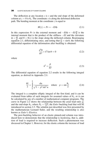
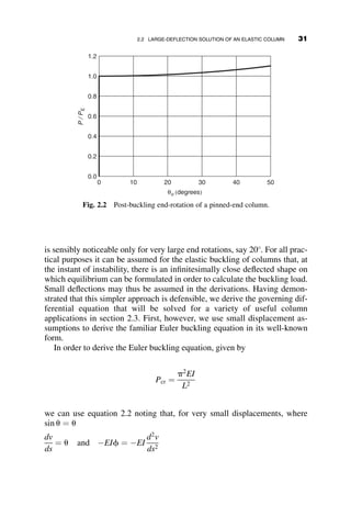
namely their stability. More precisely, it will examine how and under what
loading condition the structure will pass from a stable state to an unstable
one. The reason for this interest is that the structural engineer, knowing the
circumstances of the limit of stability, can then proportion a structural
scheme that will stay well clear of the zone of danger and will have an ad-
equate margin of safety against collapse due to instability. In a well-
designed structure, the user or occupant will never have to even think of the
structure’s existence. Safety should always be a given to the public.
Absolute safety, of course, is not an achievable goal, as is well known to
structural engineers. The recent tragedy of the World Trade Center collapse
provides understanding of how a design may be safe under any expected
circumstances, but may become unstable under extreme and unforeseeable
circumstances. There is always a small chance of failure of the structure.
The term failure has many shades of meaning. Failure can be as obvious
and catastrophic as a total collapse, or more subtle, such as a beam that suf-
fers excessive deflection, causing floors to crack and doors to not open or
close. In the context of this book, failure is defined as the behavior of the
structure when it crosses a limit state—that is, when it is at the limit of its
structural usefulness. There are many such limit states the structural design
engineer has to consider, such as excessive deflection, large rotations at
joints, cracking of metal or concrete, corrosion, or excessive vibration under
dynamic loads, to name a few. The one limit state that we will consider here
is the limit state where the structure passes from a stable to an unstable
condition.
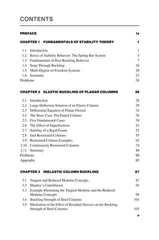
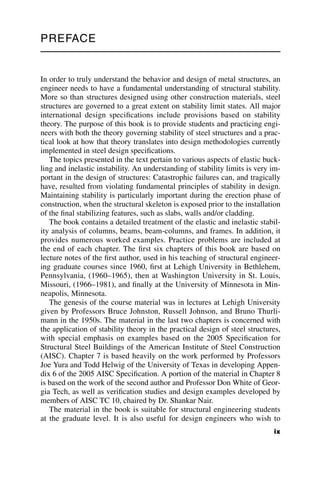
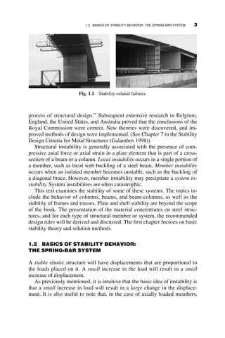
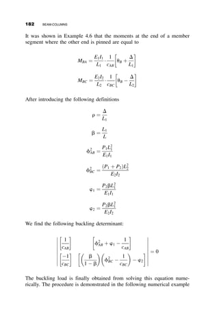
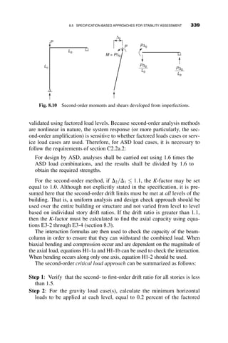
Instability failures are often catastrophic and occur most often during erec-
tion. For example, during the late 1960s and early 1970s, a number of major
steel box-girder bridges collapsed, causing many deaths among erection per-
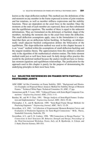
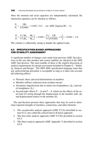
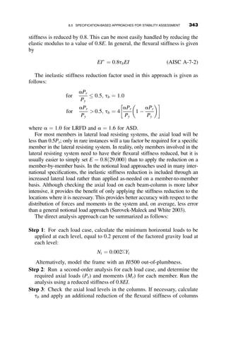
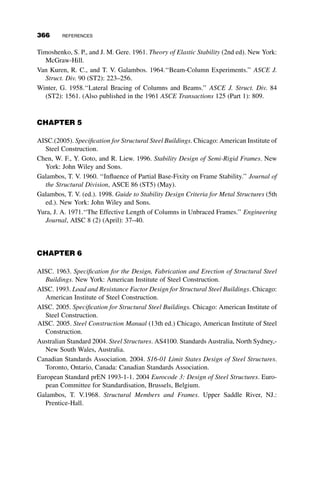
sonnel. The two photographs in Figure 1.1 were taken by author Galambos in
August 1970 on the site two months before the collapse of a portion of the
Yarra River Crossing in Melbourne, Australia. The left picture in Figure 1.1
shows two halves of the multi-cell box girder before they were jacked into
place on top of the piers (see right photo), where they were connected with
high-strength bolts. One of the 367.5 ft. spans collapsed while the iron-
workers attempted to smooth the local buckles that had formed on the top
surface of the box. Thirty-five workers and engineers perished in the disaster.
There were a number of causes for the collapse, including inexperience
and carelessness, but the Royal Commission (1971), in its report pinpointed
the main problem: ‘‘We find that [the design organization] made assump-
tions about the behavior of box girders which extended beyond the range of
engineering knowledge.’’ The Royal Commission concluded ‘‘ . . . that the
design firm ‘‘failed altogether to give proper and careful regard to the
2 FUNDAMENTALS OF STABILITY THEORY](https://image.slidesharecdn.com/structuralstabilityofsteelconceptsa-220725050455-cb14c4fb/85/STRUCTURAL_STABILITY_OF_STEEL_CONCEPTS_A-pdf-10-320.jpg)
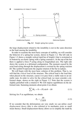
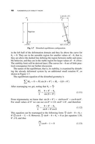
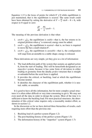
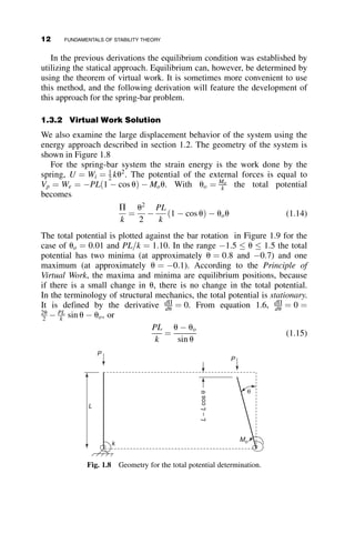
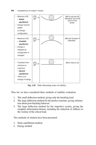
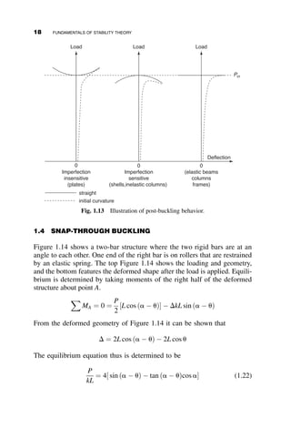
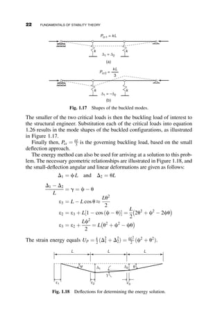
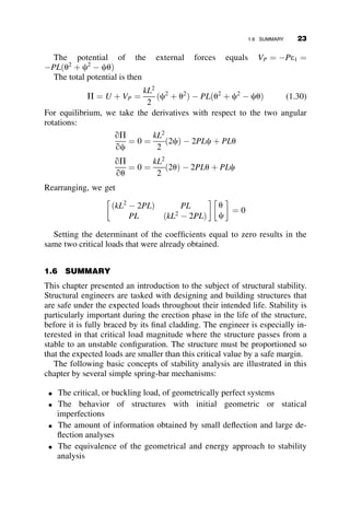
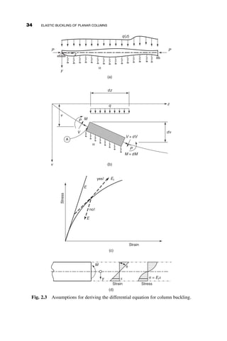
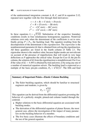
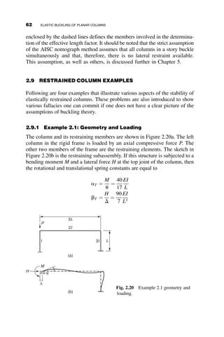
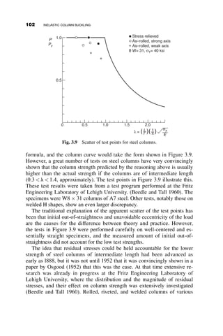
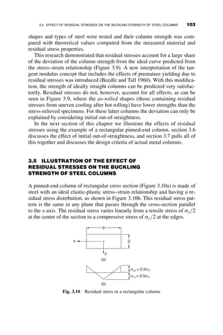
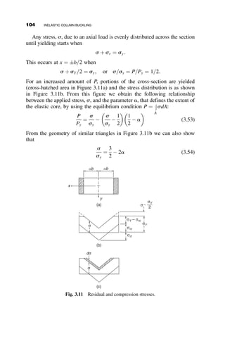
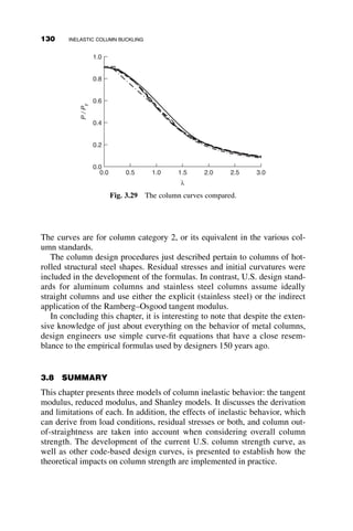
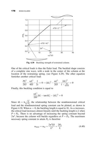
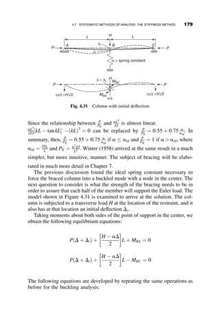
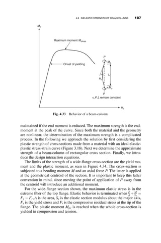
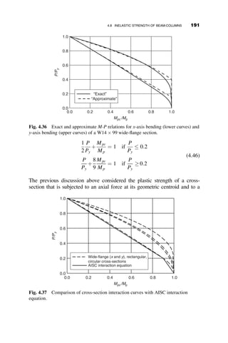
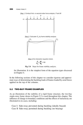
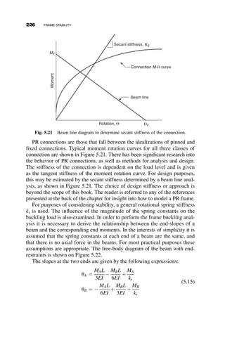
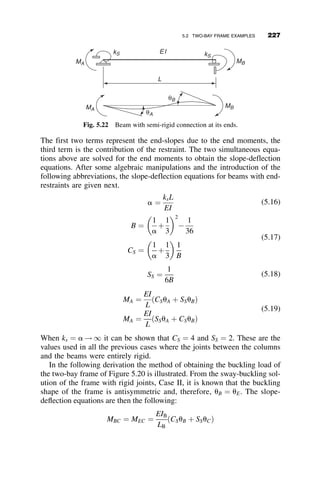
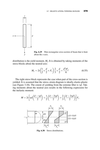
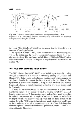


This chapter introduces fundamental concepts of stability theory that are important for structural engineers to understand. Stability is defined as a structure's ability to resist changing shape under loads through small displacements. Instability occurs when a structure is at the limit between a stable and unstable state, where small load increases cause large displacements. The chapter uses simple spring-bar systems to illustrate buckling behavior and post-buckling strength. It also discusses multi-degree of freedom systems and different types of buckling modes like snap-through. Understanding stability theory allows engineers to properly proportion structures to avoid instability failures.


![[Liang,_Qing_Quan]_Analysis_and_Design_of_Steel_an(BookZZ.org).pdf](https://cdn.slidesharecdn.com/ss_thumbnails/liangqingquananalysisanddesignofsteelanbookzz-220725050452-4cf9daa6-thumbnail.jpg?width=640&height=640&fit=bounds)