This chapter provides an introduction to matrix algebra, which forms the basis for modeling structural systems. Key concepts covered include matrix addition, subtraction, multiplication, determinants, inverses, and solving systems of equations. These matrix operations and concepts are fundamental to assembling and solving the systems of equations that describe structural behavior.


![Matrix Algebra 3
Multiplication between two matrices
C = AB (1.10)
can be performed only if the number of columns in A equals the number of rows in B. The
element Cij is then computed according to
Cij =
n
∑
k=1
AikBkj (1.11)
For
A =
[
A11 A12
A21 A22
]
; B =
[
B11 B12
B21 B22
]
(1.12)
the product of the matrices, C = AB, is obtained from
C =
[
A11 A12
A21 A22
]
[
B11 B12
B21 B22
]
=
[
A11B11 + A12B21 A11B12 + A12B22
A21B11 + A22B21 A21B12 + A22B22
]
(1.13)
In general,
BA ≠ AB (1.14)
1.4 Determinant
For every quadratic matrix A (n × n), it is possible to compute a scalar value called a determi-
nant. For n = 1,
det A = A11 (1.15)
For n > 1, the determinant det A is computed according to the expression
det A =
n
∑
k=1
(−1)i+k
Aik det Mik (1.16)
where i is an arbitrary row number and det Mik is the determinant of the matrix obtained when
the ith row and the kth column is deleted from the matrix A. For n = 2, this results in
det A = A11A22 − A12A21 (1.17)
and for n = 3
det A = A11A22A33 + A12A23A31 + A13A21A32 − A11A23A32 − A12A21A33 − A13A22A31
(1.18)
1.5 Inverse Matrix
The quadratic matrix A is invertible if there exists a matrix A−1 such that
A−1
A = I (1.19)](https://image.slidesharecdn.com/structuralmechanicsmodellingandanalysisofframesandtrussespdfdrive-230720064114-5e1f9a93/75/Structural-mechanics-_-modelling-and-analysis-of-frames-and-trusses-PDFDrive-pdf-17-2048.jpg)
![6 Structural Mechanics: Modelling and Analysis of Frames and Trusses
In the next step, we let the rows 1 and 2 remain. From row 3 we subtract row 2 multiplied
by the quotient K32∕K22 = −5∕8 = −0.625. We have triangularised the coefficient matrix
K and obtain
⎡
⎢
⎢
⎣
8 −4 −2
0 8 −5
0 0 6.375
⎤
⎥
⎥
⎦
⎡
⎢
⎢
⎣
a1
a2
a3
⎤
⎥
⎥
⎦
=
⎡
⎢
⎢
⎣
−8
14
12.75
⎤
⎥
⎥
⎦
(3)
With the system of equations in this form, we can determine a3, a2 and a1 by
back-substitution
a3 =
12.75
6.375
= 2; a2 =
14 − (−5)a3
8
= 3;
a1 =
−8 − (−4)a2 − (−2)a3
8
= 1 (4)
and with that, we have the solution
⎡
⎢
⎢
⎣
a1
a2
a3
⎤
⎥
⎥
⎦
=
⎡
⎢
⎢
⎣
1
3
2
⎤
⎥
⎥
⎦
(5)
To check the results, we can substitute the solution into the original system of equations
and carry out the matrix multiplication
⎡
⎢
⎢
⎣
8 −4 −2
−4 10 −4
−2 −4 10
⎤
⎥
⎥
⎦
⎡
⎢
⎢
⎣
1
3
2
⎤
⎥
⎥
⎦
which gives
⎡
⎢
⎢
⎣
−8
18
6
⎤
⎥
⎥
⎦
(6)
This is equal to the original right-hand side of the system of equations, that is the solution
found is correct.
1.7.2 Systems of Equations with Known and Unknown Components in the
Vector a
The systems of equations that we consider, in general, has a square matrix K, initially with
det K = 0, and a vector f ≠ 𝟎. Moreover, it is usually the case that some components of a are
known and the corresponding components of f are unknown. One systematic way to solve
such a system of equations begins with a partition of the matrices, which means that they are
divided into submatrices
K =
[
A1 A2
A3
̃
K
]
; a =
[
g
̃
a
]
; f =
[
r
̃
f
]
(1.39)
where the matrices A1, A2, A3, ̃
K, g and ̃
f contain known quantities, while ̃
a and r are unknown.
With use of these submatrices, the system of equations (1.38) can be expressed as
[
A1 A2
A3
̃
K
]
[
g
̃
a
]
=
[
r
̃
f
]
(1.40)](https://image.slidesharecdn.com/structuralmechanicsmodellingandanalysisofframesandtrussespdfdrive-230720064114-5e1f9a93/75/Structural-mechanics-_-modelling-and-analysis-of-frames-and-trusses-PDFDrive-pdf-20-2048.jpg)
![Matrix Algebra 7
The system of equations can be divided into two parts and then be written as
A1g + A2 ̃
a = r (1.41)
A3g + ̃
K̃
a = ̃
f (1.42)
or
̃
K̃
a = ̃
f − A3g (1.43)
r = A1g + A2 ̃
a (1.44)
where the right-hand side of the equation (1.43) consists of known quantities. The purpose of
the partition of the system of equations is to, within the original system of equations, find a
sub-system with det ̃
K ≠ 0, that is a system with a unique solution. The unknowns in ̃
a can then
be computed from (1.43). One way to perform this computation is to use Gaussian elimination.
Once ̃
a has been determined, r can be computed from (1.44).
Example 1.2 Solving a system of equations with both known and unknown compo-
nents in the vector a
In the system of equations
⎡
⎢
⎢
⎢
⎢
⎢
⎢
⎣
20 0 0 0 −20 0
0 15 0 −15 0 0
0 0 16 12 −16 −12
0 −15 12 24 −12 −9
−20 0 −16 −12 36 12
0 0 −12 −9 12 9
⎤
⎥
⎥
⎥
⎥
⎥
⎥
⎦
⎡
⎢
⎢
⎢
⎢
⎢
⎢
⎣
0
0
−3
0
a5
a6
⎤
⎥
⎥
⎥
⎥
⎥
⎥
⎦
=
⎡
⎢
⎢
⎢
⎢
⎢
⎢
⎣
f1
f2
f3
f4
0
−15
⎤
⎥
⎥
⎥
⎥
⎥
⎥
⎦
(1)
the vector a has known and unknown components. The solution can then be systematised
using partitioning (1.40). The auxiliary lines show this partition. The system of equations
is partitioned into two parts according to (1.41) and (1.42):
⎡
⎢
⎢
⎢
⎣
20 0 0 0
0 15 0 −15
0 0 16 12
0 −15 12 24
⎤
⎥
⎥
⎥
⎦
⎡
⎢
⎢
⎢
⎣
0
0
−3
0
⎤
⎥
⎥
⎥
⎦
+
⎡
⎢
⎢
⎢
⎣
−20 0
0 0
−16 −12
−12 −9
⎤
⎥
⎥
⎥
⎦
[
a5
a6
]
=
⎡
⎢
⎢
⎢
⎣
f1
f2
f3
f4
⎤
⎥
⎥
⎥
⎦
(2)
[
−20 0 −16 −12
0 0 −12 −9
]⎡
⎢
⎢
⎢
⎣
0
0
−3
0
⎤
⎥
⎥
⎥
⎦
+
[
36 12
12 9
]
[
a5
a6
]
=
[
0
−15
]
(3)
In the lower system of equations, there are two equations and two unknowns. If the known
terms of the system are gathered on the right-hand side of the equal sign, cf. (1.43), we
obtain
[
36 12
12 9
]
[
a5
a6
]
=
[
0
−15
]
−
[
−20 0 −16 −12
0 0 −12 −9
]⎡
⎢
⎢
⎢
⎣
0
0
−3
0
⎤
⎥
⎥
⎥
⎦
(4)](https://image.slidesharecdn.com/structuralmechanicsmodellingandanalysisofframesandtrussespdfdrive-230720064114-5e1f9a93/75/Structural-mechanics-_-modelling-and-analysis-of-frames-and-trusses-PDFDrive-pdf-21-2048.jpg)
![8 Structural Mechanics: Modelling and Analysis of Frames and Trusses
or [
36 12
12 9
]
[
a5
a6
]
=
[
−48
−51
]
(5)
From this system of equations, the unknown elements can be determined by Gaussian elim-
ination: the first row remains unchanged. From row 2 we subtract row 1 multiplied by the
quotient K21∕K11 = 12∕36 = 0.33333. In this way, we obtain
[
36 12
0 5
]
[
a5
a6
]
=
[
−48
−35
]
(6)
and the unknown a5 and a6 can be determined by back-substitution
a6 =
−35
5
= −7; a5 =
−48 − 12a6
36
= 1 (7)
[
a5
a6
]
=
[
1
−7
]
(8)
With a5 and a6 being known, the unknown coefficients in f can be determined using the
upper system of equations obtained from the partition, cf. (1.44),
⎡
⎢
⎢
⎢
⎣
f1
f2
f3
f4
⎤
⎥
⎥
⎥
⎦
=
⎡
⎢
⎢
⎢
⎣
20 0 0 0
0 15 0 −15
0 0 16 12
0 −15 12 24
⎤
⎥
⎥
⎥
⎦
⎡
⎢
⎢
⎢
⎣
0
0
−3
0
⎤
⎥
⎥
⎥
⎦
+
⎡
⎢
⎢
⎢
⎣
−20 0
0 0
−16 −12
−12 −9
⎤
⎥
⎥
⎥
⎦
[
1
−7
]
=
⎡
⎢
⎢
⎢
⎣
−20
0
20
15
⎤
⎥
⎥
⎥
⎦
(9)
and with that, all the unknowns are determined.
1.7.3 Eigenvalue Problems
At times it is of interest to study the case when det K = 0 and f = 𝟎. Mainly, two different
types of problems appear. A system of equations in the form
(A − 𝜆I)a = 𝟎 (1.45)
is referred to as an eigenvalue problem or sometimes standard eigenvalue problem. For a solu-
tion to exist, it is required that
det(A − 𝜆I) = 0 (1.46)
A system of equations in the form
(A − 𝜆B)a = 𝟎 (1.47)
is referred to as a generalised eigenvalue problem and for a solution to exist it is required that
det(A − 𝜆B) = 0 (1.48)
Solving an eigenvalue problem means that the values of 𝜆, which fulfil Equations (1.46) and
(1.48) are determined, that is the eigenvalues 𝜆i are computed. The number of eigenvalues](https://image.slidesharecdn.com/structuralmechanicsmodellingandanalysisofframesandtrussespdfdrive-230720064114-5e1f9a93/75/Structural-mechanics-_-modelling-and-analysis-of-frames-and-trusses-PDFDrive-pdf-22-2048.jpg)
![Matrix Algebra 9
𝜆i is equal to the number of unknowns in the system of equations. Two or more eigenvalues
may coincide. A symmetric matrix K with real elements has only real eigenvalues. For each
eigenvalue 𝜆i there is an eigenvectorai. The unknowns in the eigenvectorai cannot be uniquely
determined, but their relative magnitude can be computed.
If the product of two vectors bTc = 0, then the vectors b and c are orthogonal. For eigenvec-
tors, we have aT
i
aj = 0 for i ≠ j, that is any two eigenvectors are always orthogonal.
The following example shows how an eigenvalue problem is solved:
Example 1.3 Solving an eigenvalue problem
We want to find a solution to the eigenvalue problem
(A − 𝜆I)a = 𝟎 (1)
where
A =
[
5 −2
−2 8
]
(2)
The determinant of (A − 𝜆I) can be computed as
det(A − 𝜆I) = det
[
5 − 𝜆 −2
−2 8 − 𝜆
]
= (5 − 𝜆)(8 − 𝜆) − 4 = 𝜆2
− 13𝜆 + 36 (3)
When this expression is set to zero, the equation
𝜆2
− 13𝜆 + 36 = 0 (4)
is obtained. The solutions to this equation are the eigenvalues
𝜆1 = 4; 𝜆2 = 9 (5)
By substituting the computed eigenvalues into the first equation in the original system of
equations we obtain
(5 − 4)a1 − 2a2 = 0; a1 = t1
[
2
1
]
(6)
and
(5 − 9)a1 − 2a2 = 0; a2 = t2
[
1
−2
]
(7)
where t1 and t2 are arbitrary scalar multipliers, t1 ≠ 0, t2 ≠ 0. Had we substituted the eigen-
values into the second equation instead, the results would be the same. Computation of the
product of the two eigenvectors yields
aT
1 a2 = t1t2
[
2 1
]
[
1
−2
]
= 0 (8)
The fact that the product is 0 means that the eigenvectors a1 and a2 are orthogonal.](https://image.slidesharecdn.com/structuralmechanicsmodellingandanalysisofframesandtrussespdfdrive-230720064114-5e1f9a93/75/Structural-mechanics-_-modelling-and-analysis-of-frames-and-trusses-PDFDrive-pdf-23-2048.jpg)
![10 Structural Mechanics: Modelling and Analysis of Frames and Trusses
Exercises
1.1 Begin with the matrices
A =
[
2 3 −1
4 8 0
]
; B =
[
0 −2 4
1 0 2
]
; C =
⎡
⎢
⎢
⎣
1 0 3
4 2 1
3 4 1
⎤
⎥
⎥
⎦
and perform the following matrix operations manually.
(a) A + B
(b) ABT
(c) BT A
(d) AC
(e) det C
1.2 Introduce the matrices
A with dimensions 4 × 3
B with dimensions 3 × 6
C with dimensions 1 × 8
D with dimensions 6 × 1
Which of the following operations are possible to perform? For the possible operations,
give the dimensions of E
(a) E = AB
(b) E = BD
(c) E = ABCD
(d) E = ABDC
(e) E = BT AT
1.3 Solve the following system of equations manually. Check the solution.
⎡
⎢
⎢
⎣
20 1 −10
−10 3 10
5 3 5
⎤
⎥
⎥
⎦
⎡
⎢
⎢
⎣
a1
a2
a3
⎤
⎥
⎥
⎦
=
⎡
⎢
⎢
⎣
−2
4
9
⎤
⎥
⎥
⎦
1.4 Solve the following systems of equations manually and check the solutions.
(a) ⎡
⎢
⎢
⎣
4 −2 −2
−2 5 −3
−2 −3 5
⎤
⎥
⎥
⎦
⎡
⎢
⎢
⎣
0
0
a3
⎤
⎥
⎥
⎦
=
⎡
⎢
⎢
⎣
f1
f2
10
⎤
⎥
⎥
⎦
(b) ⎡
⎢
⎢
⎣
6 −4 −2
−4 12 −8
−2 −8 10
⎤
⎥
⎥
⎦
⎡
⎢
⎢
⎣
1
a2
a3
⎤
⎥
⎥
⎦
=
⎡
⎢
⎢
⎣
f1
16
−6
⎤
⎥
⎥
⎦](https://image.slidesharecdn.com/structuralmechanicsmodellingandanalysisofframesandtrussespdfdrive-230720064114-5e1f9a93/75/Structural-mechanics-_-modelling-and-analysis-of-frames-and-trusses-PDFDrive-pdf-24-2048.jpg)
![Matrix Algebra 11
(c) ⎡
⎢
⎢
⎢
⎢
⎣
4 −4 0 0 0
−4 7 −2 −1 0
0 −2 5 −3 0
0 −1 −3 7 −3
0 0 0 −3 3
⎤
⎥
⎥
⎥
⎥
⎦
⎡
⎢
⎢
⎢
⎢
⎣
−3
a2
0
a4
3
⎤
⎥
⎥
⎥
⎥
⎦
=
⎡
⎢
⎢
⎢
⎢
⎣
f1
4
f3
−1
f5
⎤
⎥
⎥
⎥
⎥
⎦
1.5 Begin with the matrices
A =
⎡
⎢
⎢
⎢
⎣
2 1 0 3
6 4 1 −2
0 3 4 1
1 2 −4 6
⎤
⎥
⎥
⎥
⎦
; B =
⎡
⎢
⎢
⎢
⎣
3 4 1 −2
6 8 1 0
2 2 3 −2
1 4 0 4
⎤
⎥
⎥
⎥
⎦
;
C =
⎡
⎢
⎢
⎢
⎣
−4
2
3
1
⎤
⎥
⎥
⎥
⎦
; D =
[
1 4 −3 6
]
and perform the following matrix operations with CALFEM. For the sub-exercises with
more than one matrix operation, compare and comment on the results.
(a) A + B and B + A
(b) AB and BA
(c) (AB)T, (BA)T and BTAT
(d) CD and DC
(e) CTAC
(f) det A, A−1 and AA−1
1.6 Compute the determinant of the matrices in the following systems of equations with
CALFEM. If possible, solve the systems of equations and check the solutions. If any of
the systems is unsolvable, explain why.
(a) ⎡
⎢
⎢
⎢
⎣
−4 3 0 1
1 2 −1 4
0 1 −1 2
2 0 2 2
⎤
⎥
⎥
⎥
⎦
⎡
⎢
⎢
⎢
⎣
a1
a2
a3
a4
⎤
⎥
⎥
⎥
⎦
=
⎡
⎢
⎢
⎢
⎣
−2
−1
−3
2
⎤
⎥
⎥
⎥
⎦
(b) ⎡
⎢
⎢
⎣
4 −4 0
−4 6 −2
0 −2 2
⎤
⎥
⎥
⎦
⎡
⎢
⎢
⎣
a1
a2
a3
⎤
⎥
⎥
⎦
=
⎡
⎢
⎢
⎣
0
0
0
⎤
⎥
⎥
⎦
(c) ⎡
⎢
⎢
⎣
8 −3 −5
−3 5 −2
−5 −2 7
⎤
⎥
⎥
⎦
⎡
⎢
⎢
⎣
a1
a2
a3
⎤
⎥
⎥
⎦
=
⎡
⎢
⎢
⎣
4
2
−6
⎤
⎥
⎥
⎦
1.7 Consider the eigenvalue problem (A − 𝜆I)a = 𝟎, where
A =
[
10 −3
−3 2
]
(a) Compute the eigenvalues.
(b) Compute the eigenvectors and check that they are orthogonal.](https://image.slidesharecdn.com/structuralmechanicsmodellingandanalysisofframesandtrussespdfdrive-230720064114-5e1f9a93/75/Structural-mechanics-_-modelling-and-analysis-of-frames-and-trusses-PDFDrive-pdf-25-2048.jpg)

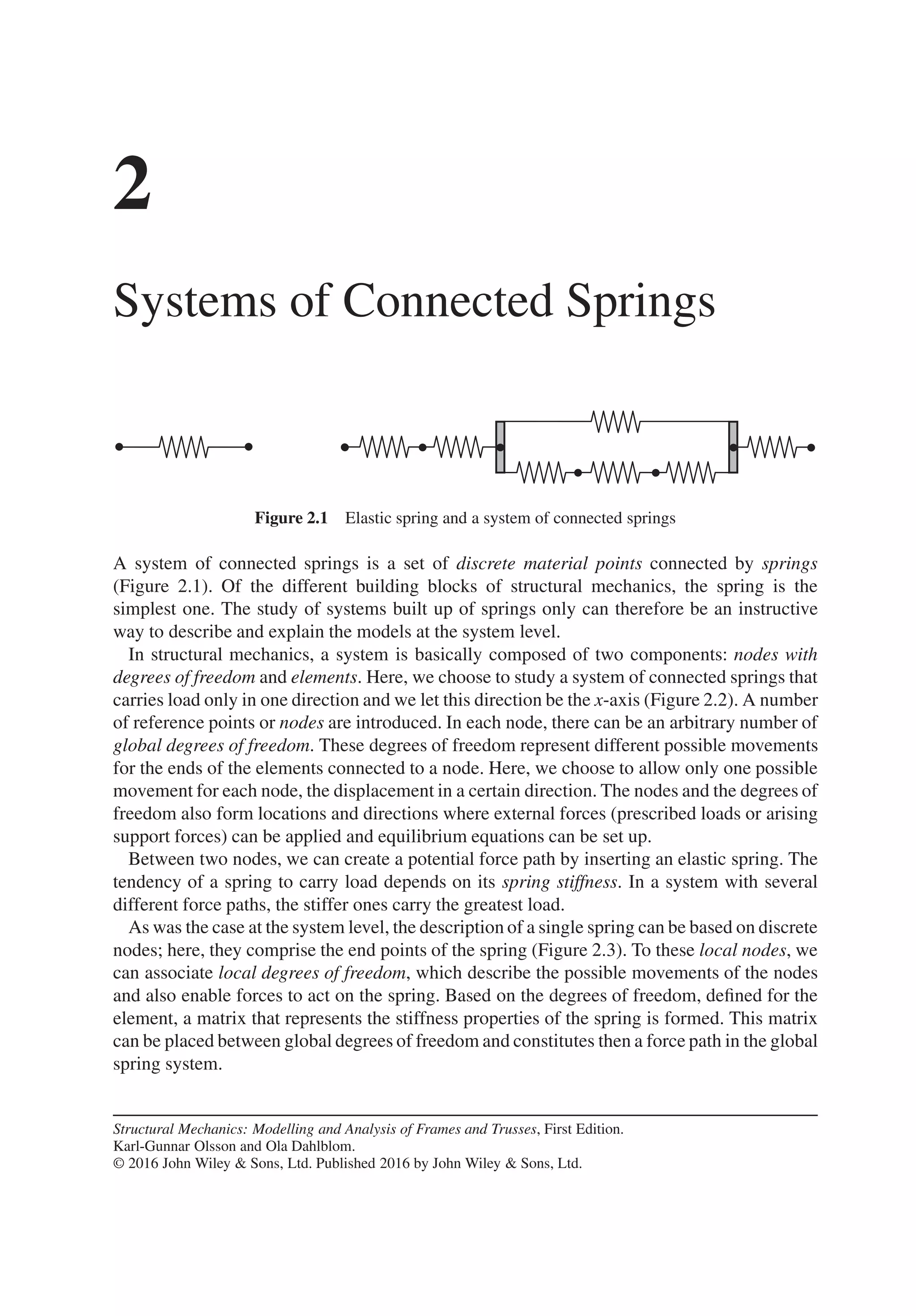
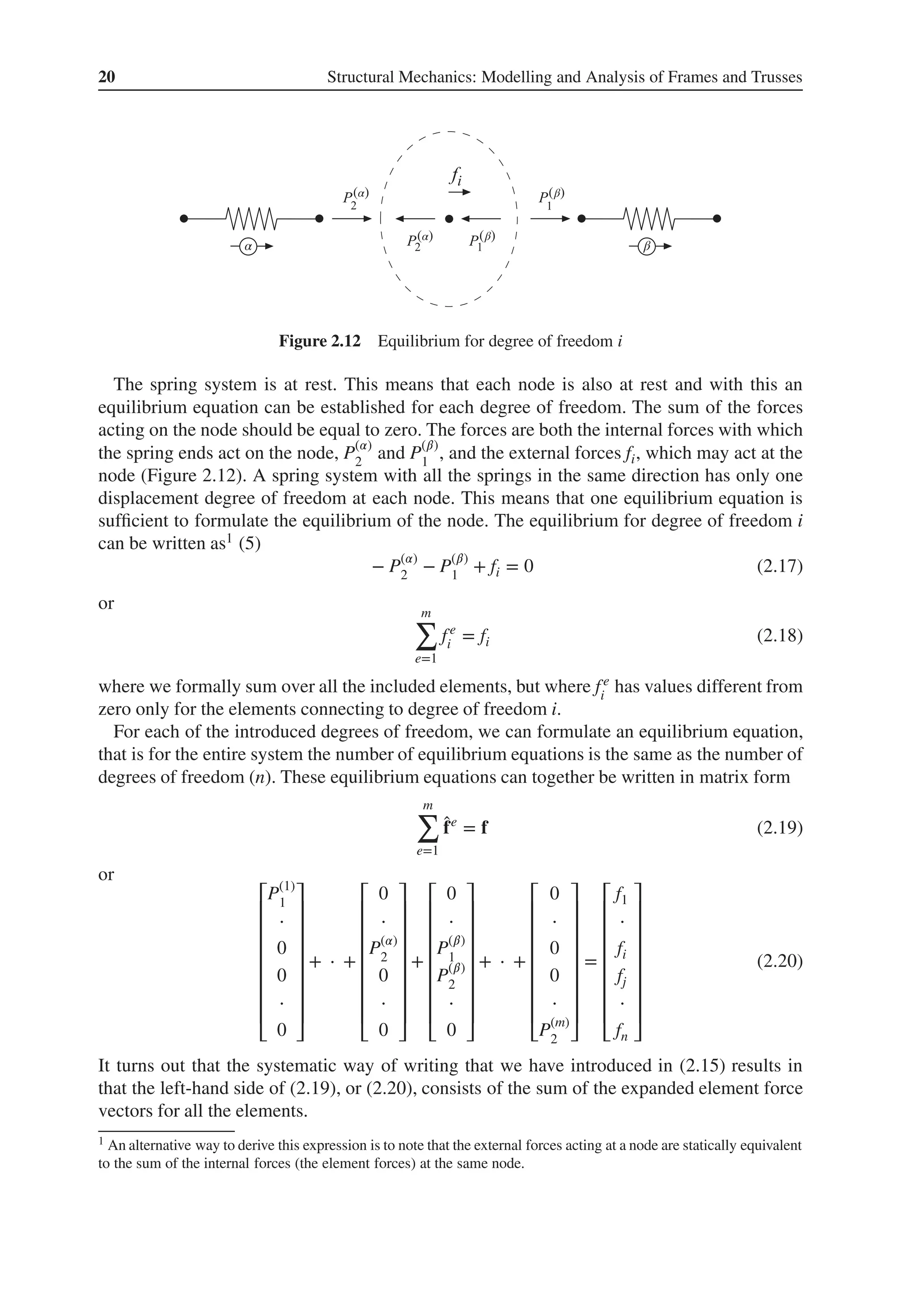
![Systems of Connected Springs 17
P1 = −N (2.4)
P2 = N
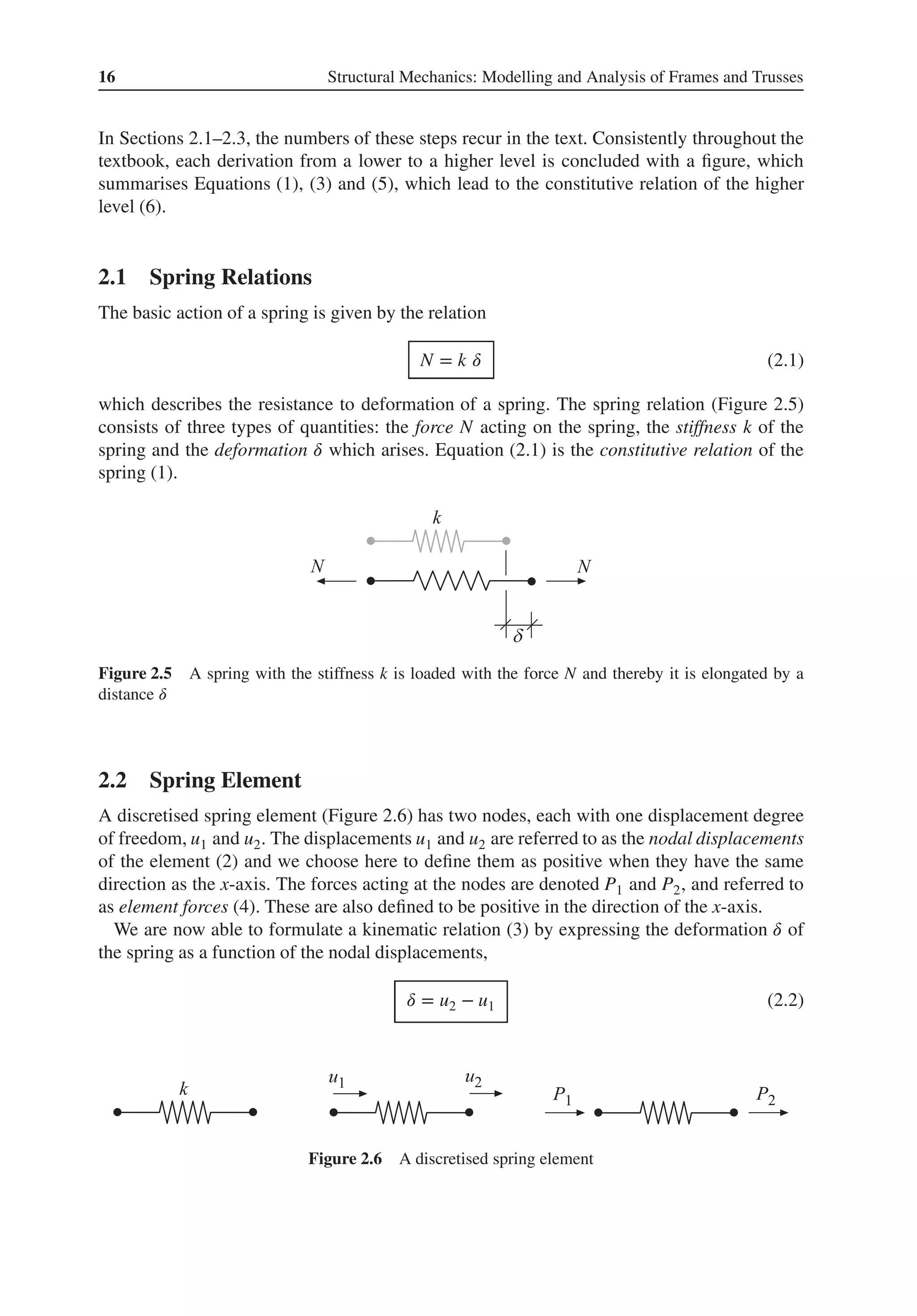
N = k 𝛿 (2.1)
𝛿 = u2 − u1 (2.2)
⎫
⎪
⎪
⎬
⎪
⎪
⎭
⇒ Ke
ae
= fe
(2.7)
where
Ke
= k
[
1 −1
−1 1
]
; ae
=
[
u1
u2
]
; fe
=
[
P1
P2
]
Figure 2.7 From spring to spring element
By substituting (2.2) into (2.1), we can express the spring force as
N = k(u2 − u1) (2.3)
For a spring to be in equilibrium, two forces that are equal in magnitude and opposite in
direction must be acting on the spring, one at each end. If we compare the definition of the
spring force N (Figure 2.5) with the definition of the element forces P1 and P2 (Figure 2.6),
we observe (5) that
P1 = −N; P2 = N (2.4)
Substituting (2.4) into (2.3) gives
P1 = −k(u2 − u1) (2.5)
P2 = k(u2 − u1) (2.6)
or, in matrix form
Ke
ae
= fe
(2.7)
where
fe
=
[
P1
P2
]
; Ke
= k
[
1 −1
−1 1
]
; ae
=
[
u1
u2
]
(2.8)
The relation (2.7) is the constitutive relation (6) of the spring and is referred to as the element
equation of the spring where Ke is the element stiffness matrix, ae the element displacement
vector and fe the element force vector. The index e is used to denote that the relation is for a
single element.
A summary of the relations, which lead to the element equation of the spring, is shown in
Figure 2.7.
2.3 Systems of Springs
With the spring element (1) described in (2.7), we can now construct and analyse complex
systems of connected springs (Figure 2.8). The aim is to establish a constitutive relation for
the entire spring system. We begin by defining the degrees of freedom in a global coordinate](https://image.slidesharecdn.com/structuralmechanicsmodellingandanalysisofframesandtrussespdfdrive-230720064114-5e1f9a93/75/Structural-mechanics-_-modelling-and-analysis-of-frames-and-trusses-PDFDrive-pdf-31-2048.jpg)
![18 Structural Mechanics: Modelling and Analysis of Frames and Trusses
Figure 2.8 A system of connected springs
system, and introducing a global numbering of all the degrees of freedom, from 1 to n. These
displacements are gathered in a global displacement vector a (2).
a =
⎡
⎢
⎢
⎢
⎢
⎢
⎢
⎣
a1
⋅
ai
aj
⋅
an
⎤
⎥
⎥
⎥
⎥
⎥
⎥
⎦
(2.9)
The next step is to put each of the spring elements into the global system. In a given global
system, each element has its defined position with defined connections to the degrees of free-
dom of the global system. For example, the local displacements u1 and u2 of the element 𝛽
correspond to the global degrees of freedom ai and aj (Figure 2.9), that is
u1 = ai (2.10)
u2 = aj (2.11)
These relations describe how the spring elements are connected physically in the global
system. The relations are a type of kinematic relations referred to as compatibility
requirements (3). These compatibility requirements can be written in matrix form as
ae
= Ha (2.12)
where ae is defined in (2.8), a in (2.9) and where
H =
[
0 ⋅ 1 0 ⋅ 0
0 ⋅ 0 1 ⋅ 0
]
(2.13)
β
β
Figure 2.9 Global and local displacements](https://image.slidesharecdn.com/structuralmechanicsmodellingandanalysisofframesandtrussespdfdrive-230720064114-5e1f9a93/75/Structural-mechanics-_-modelling-and-analysis-of-frames-and-trusses-PDFDrive-pdf-32-2048.jpg)
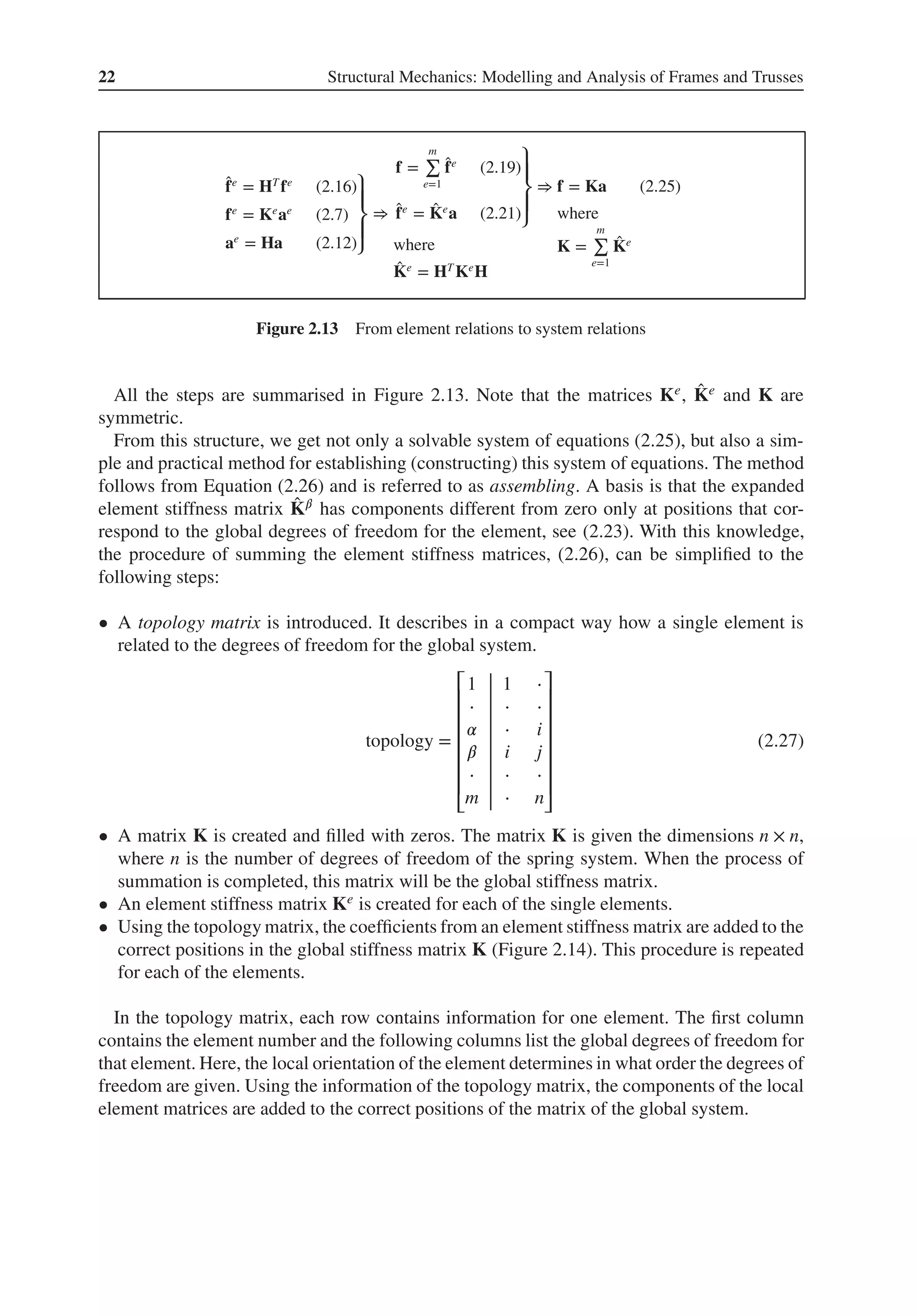
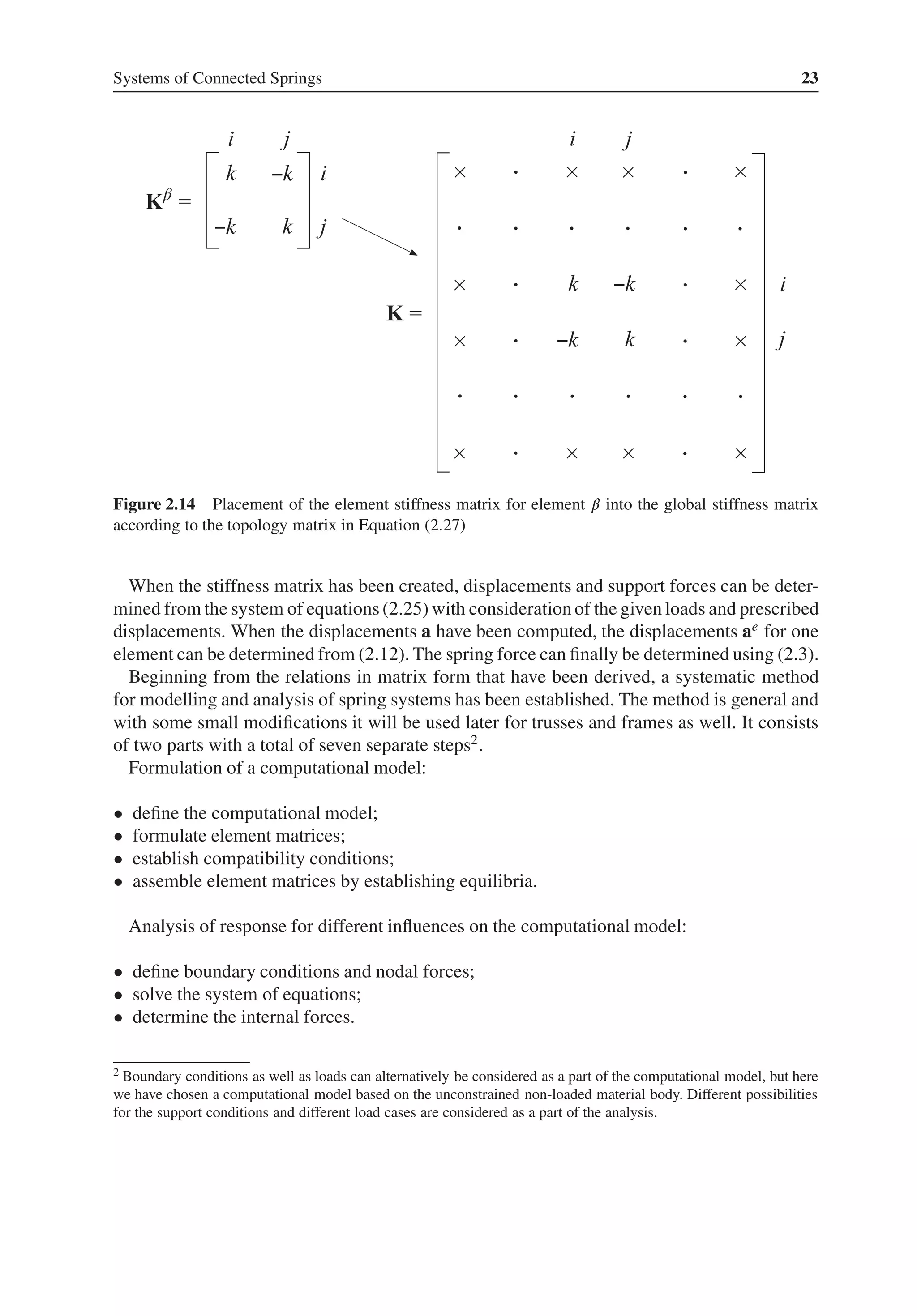
![Systems of Connected Springs 21
The expanded element force vector for an element is related to the local element force vector
through (2.16). Substituting the constitutive relation (2.7) and the compatibility requirements
(2.12) into (2.16), we can write the expanded element force vector as
̂
fe
= ̂
Ke
a (2.21)
where
̂
Ke
= HT
Ke
H (2.22)
̂
Ke is referred to as the expanded element stiffness matrix and shows where in a global system
the stiffness of an element should be placed. For a spring element 𝛽, the expanded element
stiffness matrix is obtained from
̂
K𝛽
= k
⎡
⎢
⎢
⎢
⎢
⎢
⎢
⎣
0 0
⋅ ⋅
1 0
0 1
⋅ ⋅
0 0
⎤
⎥
⎥
⎥
⎥
⎥
⎥
⎦
[
1 −1
−1 1
]
[
0 ⋅ 1 0 ⋅ 0
0 ⋅ 0 1 ⋅ 0
]
= k
⎡
⎢
⎢
⎢
⎢
⎢
⎢
⎣
0 ⋅ 0 0 ⋅ 0
⋅ ⋅ ⋅ ⋅ ⋅ ⋅
0 ⋅ 1 −1 ⋅ 0
0 ⋅ −1 1 ⋅ 0
⋅ ⋅ ⋅ ⋅ ⋅ ⋅
0 ⋅ 0 0 ⋅ 0
⎤
⎥
⎥
⎥
⎥
⎥
⎥
⎦
(2.23)
Substituting (2.21) into the equilibrium relation (2.19) gives
m
∑
e=1
̂
Ke
a = f (2.24)
or
Ka = f (2.25)
where
K =
m
∑
e=1
̂
Ke
(2.26)
The sequence of relations, from the local element relation (2.7) to the global relation for the
spring system (2.25), shows a general structure that will appear throughout the textbook. Even
if the contents are different for different types of problems, the same matrix notations are used.
Thus, in summary,
1. We have started from the element relation of the spring (2.7).
2. We have introduced a global displacement vector (2.9).
3. We have related local displacements to global ones using compatibility (2.12).
4. We have introduced a global vector for external loads that act on the nodes of the system
(2.14).
5. With an expanded way of writing (2.16) and using equilibrium conditions, we have related
local internal forces to global external forces (2.19).
6. With the compatibility requirements (2.12), the constitutive relation of the element (2.7)
and the expanded way of writing element forces (2.16), we have derived an expression that
describes a single element in a global system (2.21). By substituting the expanded element
relations (2.21) into the global equilibrium relations (2.19) for all the elements, we derived
a global constitutive relation for the spring system (2.25).](https://image.slidesharecdn.com/structuralmechanicsmodellingandanalysisofframesandtrussespdfdrive-230720064114-5e1f9a93/75/Structural-mechanics-_-modelling-and-analysis-of-frames-and-trusses-PDFDrive-pdf-35-2048.jpg)
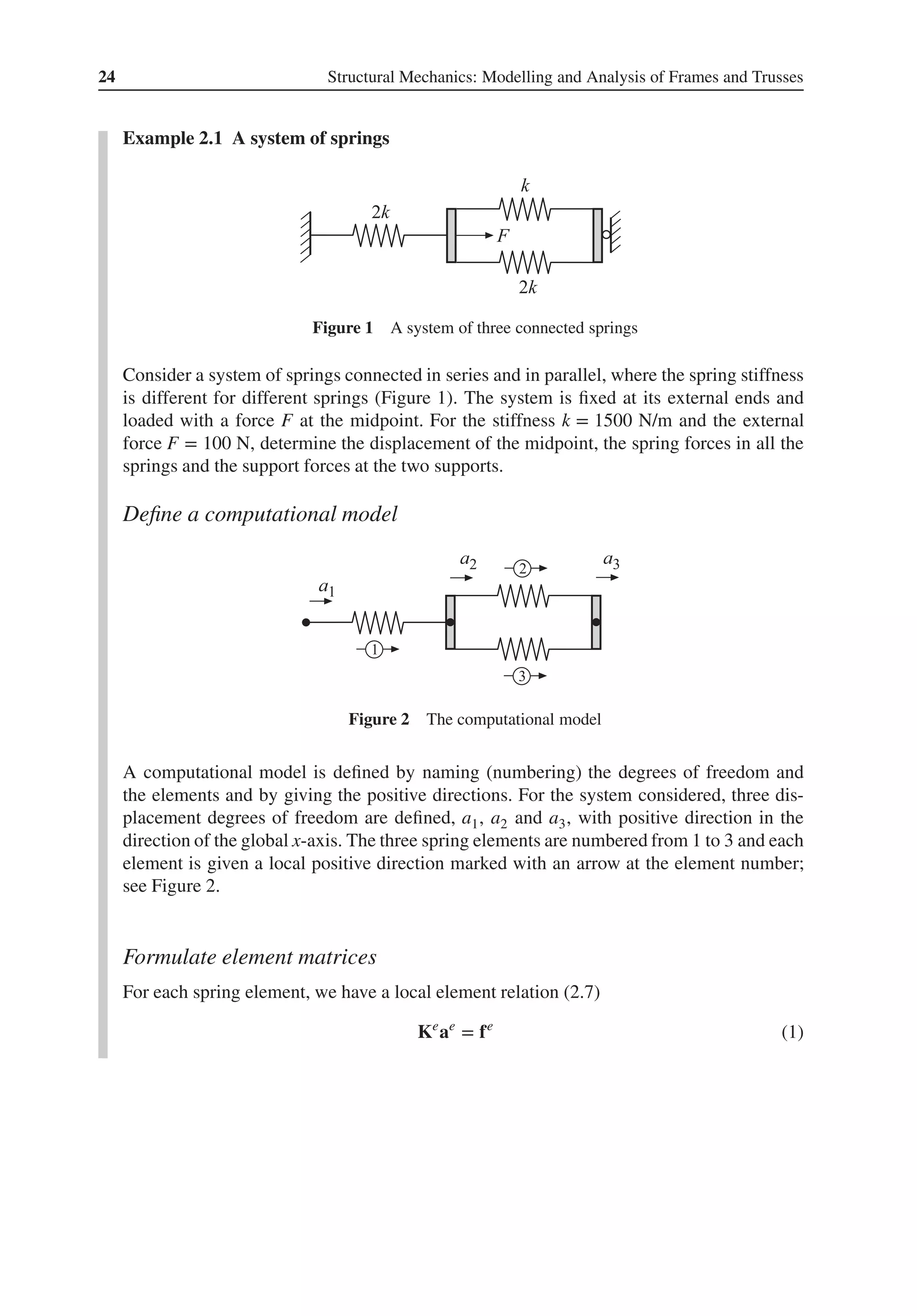
![Systems of Connected Springs 25
With k = 1500 N/m, we obtain for the three elements:
Element 1: [
P(1)
1
P(1)
2
]
=
[
3000 −3000
−3000 3000
]
[
u(1)
1
u(1)
2
]
(2)
Element 2: [
P(2)
1
P(2)
2
]
=
[
1500 −1500
−1500 1500
]
[
u(2)
1
u(2)
2
]
(3)
Element 3: [
P(3)
1
P(3)
2
]
=
[
3000 −3000
−3000 3000
]
[
u(3)
1
u(3)
2
]
(4)
Compatibility conditions
The spring system has the global displacement vector
a =
⎡
⎢
⎢
⎣
a1
a2
a3
⎤
⎥
⎥
⎦
(5)
The local degrees of freedom for Elements 1–3 correspond to global degrees of freedom
according to the following:
Element 1:
u(1)
1
= a1; u(1)
2
= a2 (6)
Element 2:
u(2)
1
= a2; u(2)
2
= a3 (7)
Element 3:
u(3)
1
= a2; u(3)
2
= a3 (8)
From the compatibility conditions, we have now obtained a description of how the ele-
ments of the spring system are connected to the degrees of freedom for the system. This
description is summarised in a topology matrix
topology =
⎡
⎢
⎢
⎣
1 1 2
2 2 3
3 2 3
⎤
⎥
⎥
⎦
(9)
Using the compatibility conditions (2.12) and the expanded element matrices, (2.7) can be
written in expanded form (2.21). For the three spring elements, the following is obtained:](https://image.slidesharecdn.com/structuralmechanicsmodellingandanalysisofframesandtrussespdfdrive-230720064114-5e1f9a93/75/Structural-mechanics-_-modelling-and-analysis-of-frames-and-trusses-PDFDrive-pdf-39-2048.jpg)
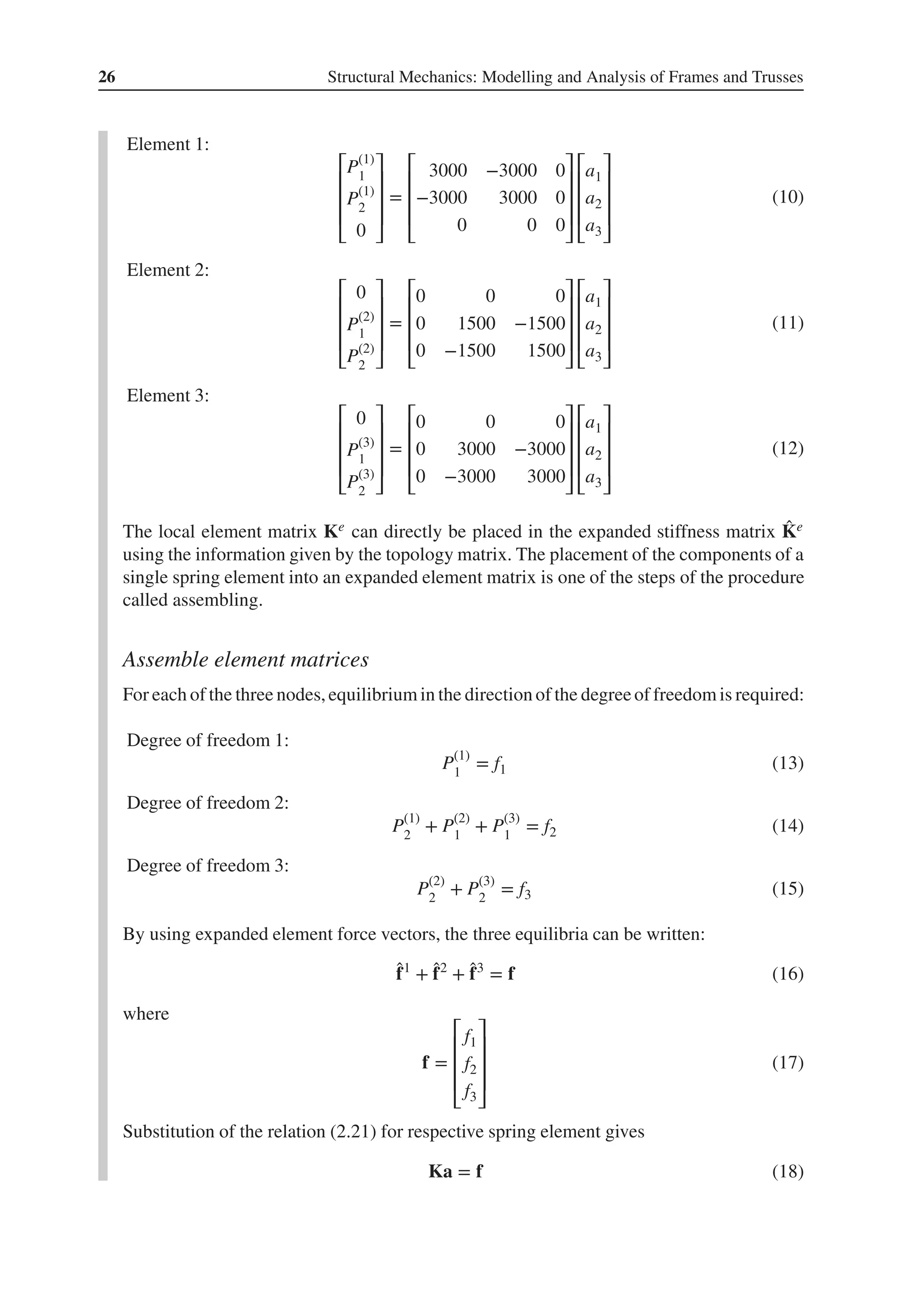
![Systems of Connected Springs 27
where
K = ̂
K1
+ ̂
K2
+ ̂
K3
(19)
With the matrix components printed out, we obtain
K =
⎡
⎢
⎢
⎣
3000 −3000 0
−3000 3000 0
0 0 0
⎤
⎥
⎥
⎦
+
⎡
⎢
⎢
⎣
0 0 0
0 1500 −1500
0 −1500 1500
⎤
⎥
⎥
⎦
+
⎡
⎢
⎢
⎣
0 0 0
0 3000 −3000
0 −3000 3000
⎤
⎥
⎥
⎦
(20)
or
K =
⎡
⎢
⎢
⎣
3000 −3000 0
−3000 7500 −4500
0 −4500 4500
⎤
⎥
⎥
⎦
(21)
By establishing equilibria for all nodes, the stiffness matrix K of the spring system is
obtained as a sum of the expanded element stiffness matrices, (2.26). This summation can
be developed into a systematic process for adding local element matrices to a matrix for
the global system. We can now express the system of equations (18) as
⎡
⎢
⎢
⎢
⎣
3000 −3000 0
−3000 7500 −4500
0 −4500 4500
⎤
⎥
⎥
⎥
⎦
⎡
⎢
⎢
⎢
⎣
a1
a2
a3
⎤
⎥
⎥
⎥
⎦
=
⎡
⎢
⎢
⎢
⎣
f1
f2
f3
⎤
⎥
⎥
⎥
⎦
(22)
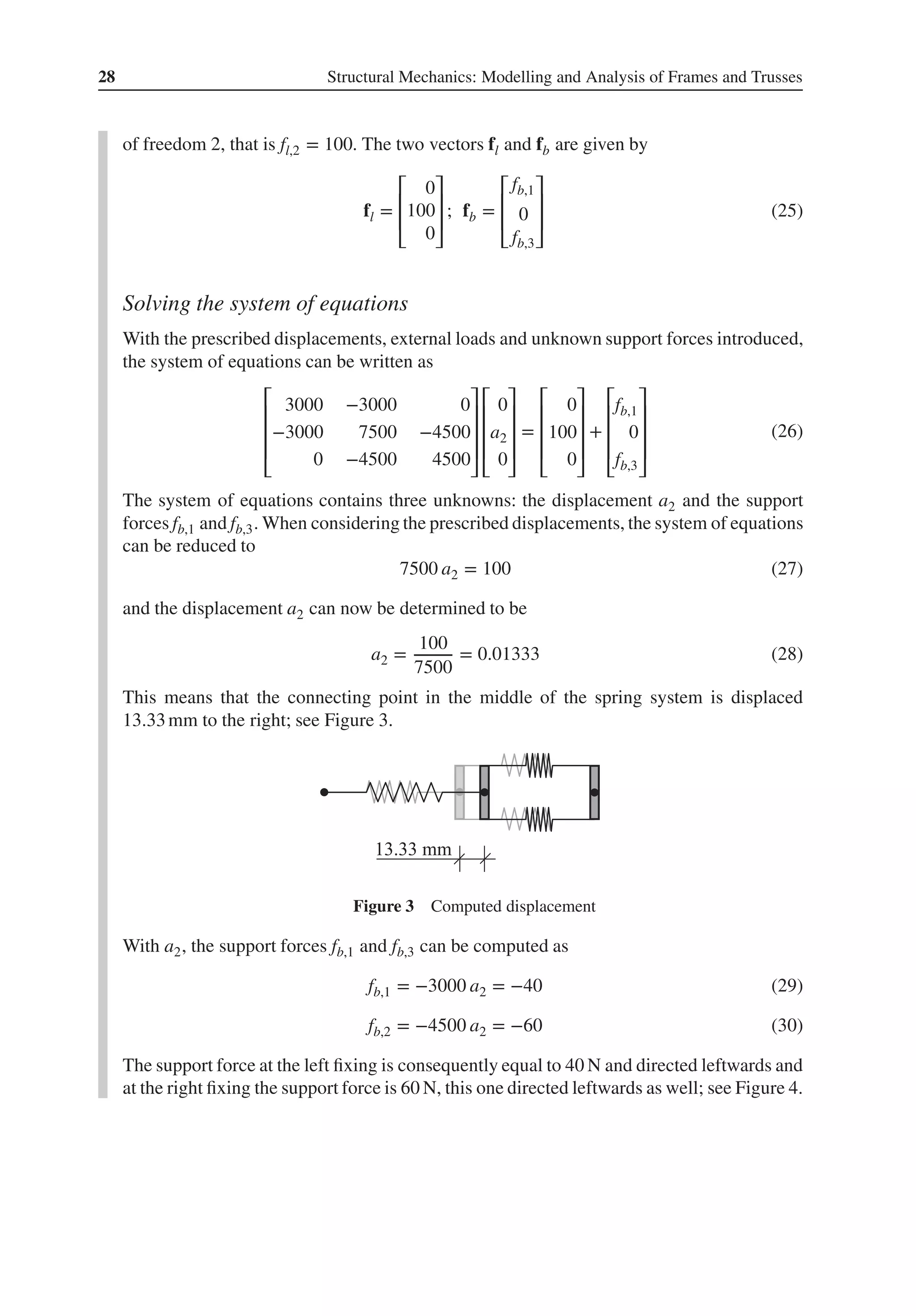
Define boundary conditions and loads
So far, the computational model has developed into a complete description of the properties
of the spring system through the fact that the components of the stiffness matrix K are now
determined. The model has also defined a possibility to prescribe different displacements
a and different external loadings f for which the response of the spring system can be
examined. As long as no displacements have been prescribed, the model describes a system
of springs that is not fixed to its surroundings, the system floats freely in a one-dimensional
space. The determinant of the system matrix K is zero. For a computation of displacements
and internal forces, boundary conditions and loads have to be defined. Our spring system
is fixed at its outer ends, that is a1 = 0 and a3 = 0. This can be described by the boundary
condition matrix
boundary conditions (bc) =
[
1 0
3 0
]
(23)
where the first column gives the degree of freedom at which the displacement should be
prescribed and the second column gives the value it should be given. By splitting the force
vector f and expressing it as the sum of two vectors, we can distinguish loads fl (l is an
abbreviation of load) from support forces fb (b is an abbreviation of boundary).
f = fl + fb (24)
At the degrees of freedom where displacement is prescribed, support forces will arise,
which we denote by fb,1 and fb,3. The spring system is loaded with the force 100 N in degree](https://image.slidesharecdn.com/structuralmechanicsmodellingandanalysisofframesandtrussespdfdrive-230720064114-5e1f9a93/75/Structural-mechanics-_-modelling-and-analysis-of-frames-and-trusses-PDFDrive-pdf-41-2048.jpg)
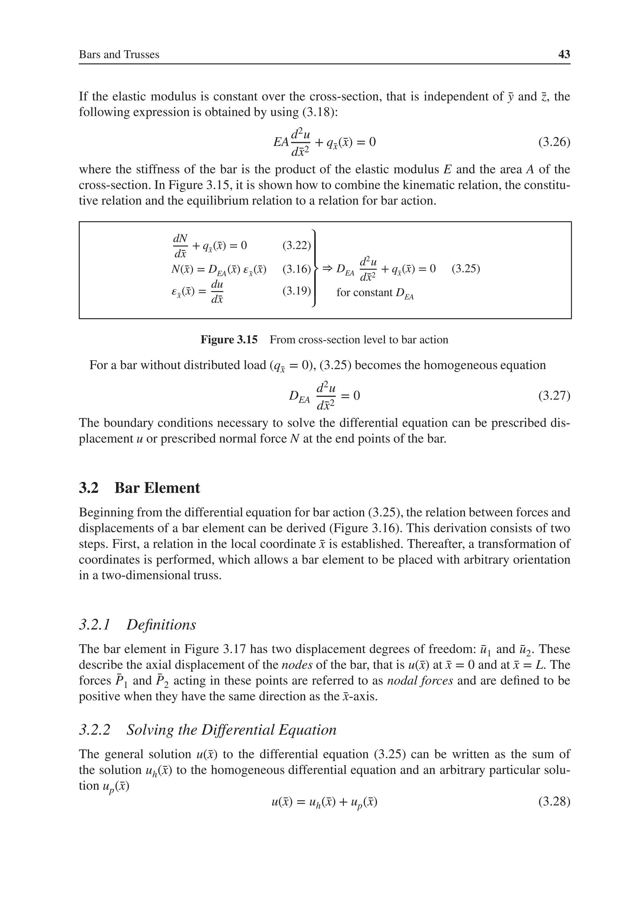
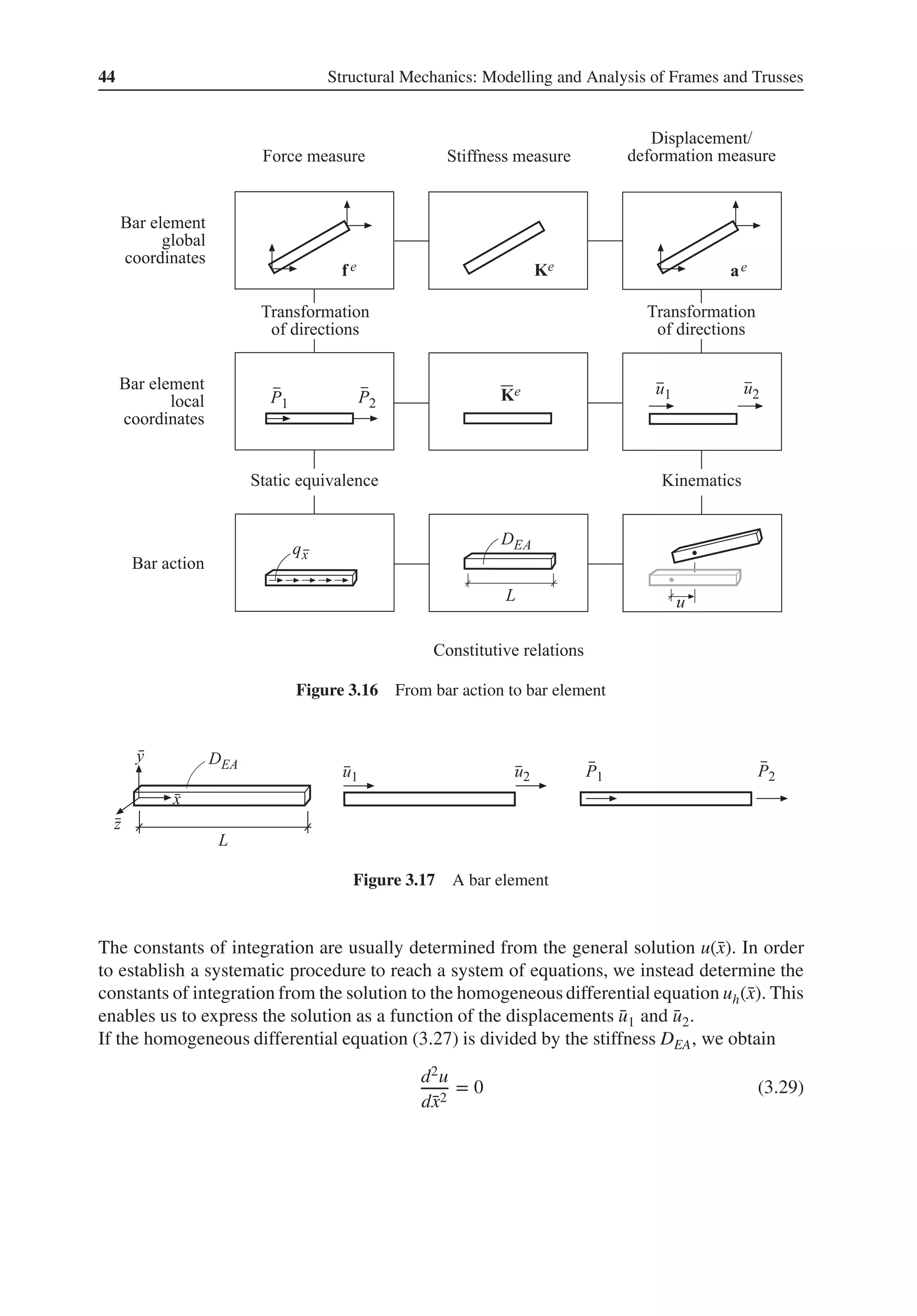
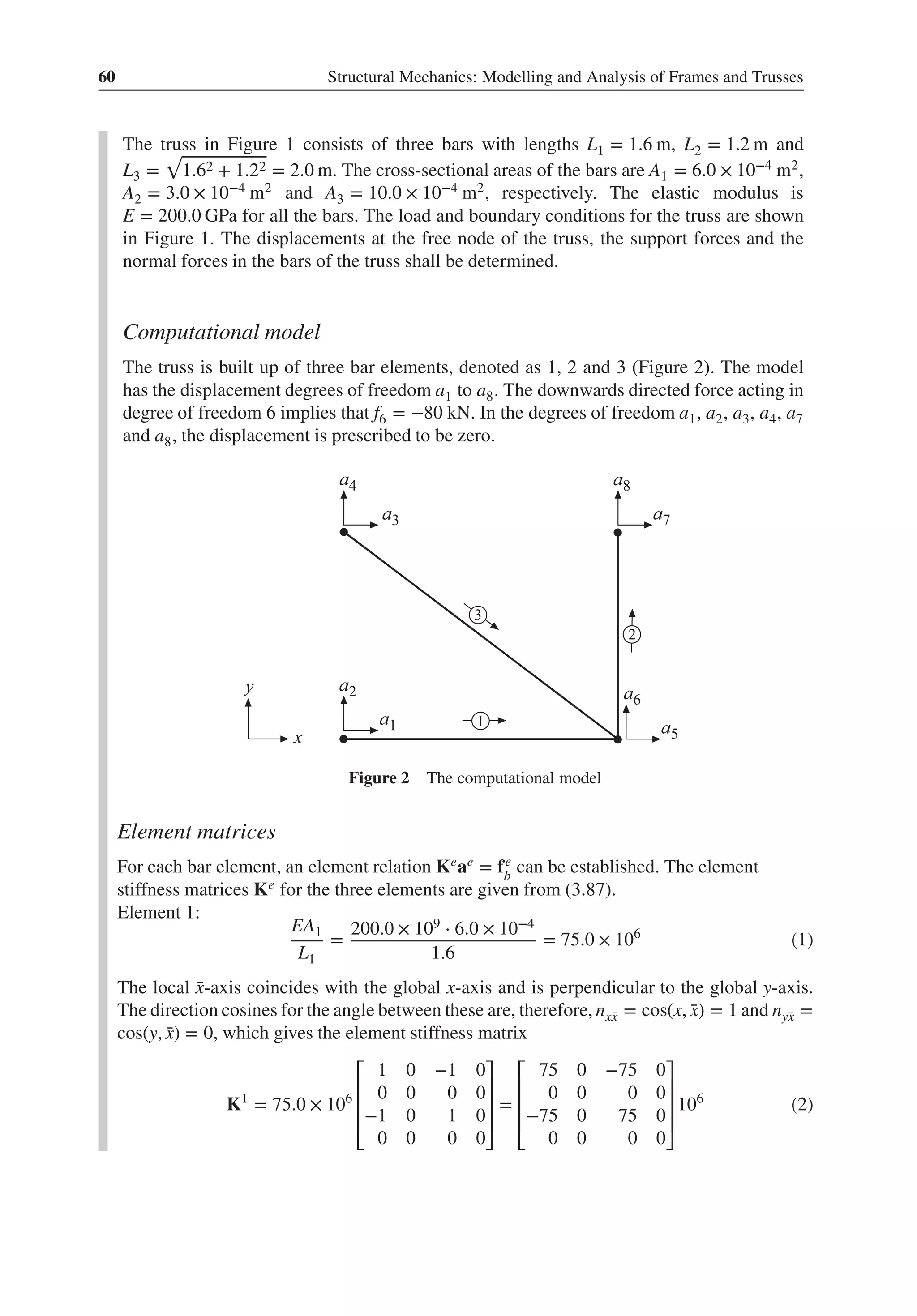
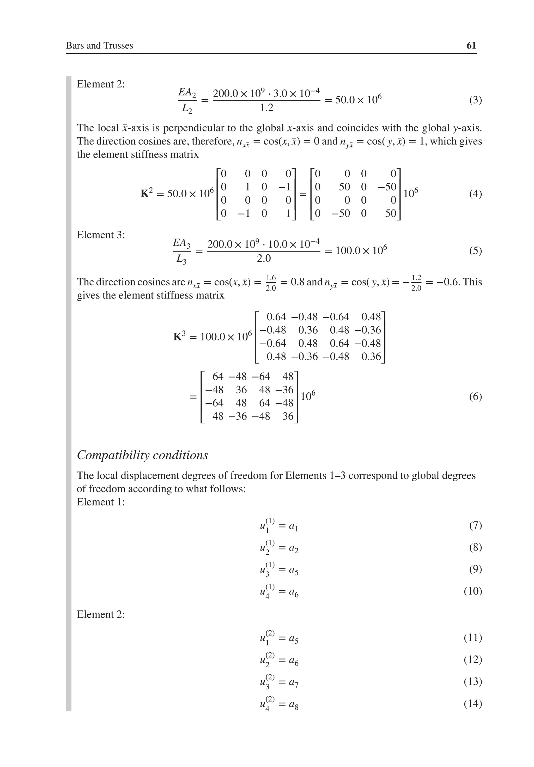
![Bars and Trusses 45
Integrating twice gives
uh(̄
x) = 𝛼1 + 𝛼2 ̄
x (3.30)
or in matrix form
uh(̄
x) = ̄
N𝛂 (3.31)
where ̄
N = ̄
N(̄
x) describes how the solution varies along the ̄
x-axis and 𝛂 contains the constants
of integration,
̄
N =
[
1 ̄
x
]
; 𝛂 =
[
𝛼1
𝛼2
]
(3.32)
At the nodes of the bar, at ̄
x = 0 and ̄
x = L, the boundary conditions
uh(0) = ̄
u1 (3.33)
uh(L) = ̄
u2 (3.34)
apply. These conditions when substituted into (3.31) give
̄
u1 = 𝛼1 (3.35)
̄
u2 = 𝛼1 + 𝛼2L (3.36)
or in matrix form
̄
ae
= C𝛂 (3.37)
where
̄
ae
=
[
̄
u1
̄
u2
]
; C =
[
1 0
1 L
]
(3.38)
By inverting C, we can express the constants of integration 𝛂 as functions of the displacement
degrees of freedom of the element ̄
ae, that is as
𝛂 = C−1
̄
ae
(3.39)
where
C−1
=
[
1 0
−1
L
1
L
]
(3.40)
Substituting (3.39) into (3.31), we get the solution uh(̄
x)
uh(̄
x) = N̄
ae
(3.41)
where
N = ̄
NC−1
=
[
1 ̄
x
]
[
1 0
−1
L
1
L
]
=
[
1 − ̄
x
L
̄
x
L
]
(3.42)](https://image.slidesharecdn.com/structuralmechanicsmodellingandanalysisofframesandtrussespdfdrive-230720064114-5e1f9a93/75/Structural-mechanics-_-modelling-and-analysis-of-frames-and-trusses-PDFDrive-pdf-59-2048.jpg)
![46 Structural Mechanics: Modelling and Analysis of Frames and Trusses
With that, we have reformulated uh(̄
x) written as a general polynomial (3.30) to a solution in
the form
uh(̄
x) = N̄
ae
= N1(̄
x)̄
u1 + N2(̄
x)̄
u2 (3.43)
where
N1(̄
x) = 1 −
̄
x
L
(3.44)
N2(̄
x) =
̄
x
L
(3.45)
The functions N1(̄
x) and N2(̄
x) describe how the solution varies with ̄
x and are referred to as
base functions or shape functions.3 We have in (3.43) an expression where the product Ni(̄
x) ̄
ui
contributes to uh(̄
x) from the displacement ̄
ui and where Ni(̄
x) states its shape and ̄
ui its size.
Substitution of (3.43) into the general solution (3.28) gives
u(̄
x) = N̄
ae
+ up(̄
x) (3.46)
where the particular solution up(̄
x) is different for different axial loadings of the bar.
Since we have chosen the constants of integration of the general solution to be equal to the
constants of integration of the solution to the homogeneousequation, there is only one possible
particular solution, namely the one where the solution is unaffected by the displacements of
the nodes, that is these displacements are equal to zero
up(0) = 0 (3.47)
up(L) = 0 (3.48)
With this systematics, the general solution u(̄
x) can be understood as the sum of the displace-
ment uh(̄
x) of a bar displaced at its ends, but otherwise non-loaded and the displacement up(̄
x)
of an axially loaded bar fixed at both ends (Figure 3.18). In Example 3.1, it is shown how to
find the particular solution for a bar with a uniformly distributed load.
Differentiation of (3.46) gives
du
d̄
x
= B̄
ae
+
dup
d̄
x
(3.49)
where
B =
dN
d̄
x
=
d ̄
N
d̄
x
C−1
=
[
0 1
]
[
1 0
−1
L
1
L
]
=
1
L
[
−1 1
]
(3.50)
Substitution of (3.49) into the expression for the normal force of the bar element (3.23) gives
N(̄
x) = DEA
(
B̄
ae
+
dup
d̄
x
)
(3.51)
or
N(̄
x) = DEAB̄
ae
+ Np(̄
x) (3.52)
3 The base functions (shape functions) that are components of the matrix N are denoted N1(̄
x) and N2(̄
x) and should
not be mistaken for the normal force, denoted N(̄
x).](https://image.slidesharecdn.com/structuralmechanicsmodellingandanalysisofframesandtrussespdfdrive-230720064114-5e1f9a93/75/Structural-mechanics-_-modelling-and-analysis-of-frames-and-trusses-PDFDrive-pdf-60-2048.jpg)
![Bars and Trusses 47
( )
( )
( )
Figure 3.18 The solution of the differential equation
where
Np(̄
x) = DEA
dup
d̄
x
(3.53)
The definitions we have introduced for forces acting at the nodes of the element give
̄
P1 = −N(0); ̄
P2 = N(L) (3.54)
Substitution of (3.52) gives the nodal forces
̄
P1 = −DEAB̄
ae
− Np(0) (3.55)
̄
P2 = DEAB̄
ae
+ Np(L) (3.56)
With
̄
fe
b =
[
̄
P1
̄
P2
]
; ̄
Ke
=
DEA
L
[
1 −1
−1 1
]
; ̄
fe
p =
[
−Np(0)
Np(L)
]
(3.57)
the Equations (3.55) and (3.56) can be written in matrix form
̄
fe
b = ̄
Ke
̄
ae
+ ̄
fe
p (3.58)
The left-hand side of the system of equations contains the nodal forces of the element ̄
fe
b
, that
is the normal forces that act on both the ends of the element. On the right-hand side, these](https://image.slidesharecdn.com/structuralmechanicsmodellingandanalysisofframesandtrussespdfdrive-230720064114-5e1f9a93/75/Structural-mechanics-_-modelling-and-analysis-of-frames-and-trusses-PDFDrive-pdf-61-2048.jpg)
![48 Structural Mechanics: Modelling and Analysis of Frames and Trusses
normal forces are divided into two parts. The product ̄
Ke ̄
ae gives the part of the normal forces
that is generated by the displacements of the end points and the vector ̄
fe
p gives the part of the
normal forces that is generated by the axial load q̄
x(̄
x). The division of the normal forces of
the bar into two parts is illustrated in Figure 3.19. Since the particular solution is determined
using the conditions that up(0) = 0 and up(L) = 0, (3.47) and (3.48), the components of ̄
fe
p can
be interpreted as the support forces that arise for a bar clamped at the ends.
To prepare for a systematic handling of loads, we now introduce an element load vector ̄
fe
l
,
̄
fe
l = −̄
fe
p =
[
Np(0)
−Np(L)
]
(3.59)
where the terms of ̄
fe
l
can be interpreted as statically equivalent resulting forces to the axial load
q̄
x(̄
x). These resulting forces act on the free-body nodes at the end points of the bar element
(Figure 3.20).
Thereby, we can write (3.58) as
̄
Ke
̄
ae
= ̄
fe
(3.60)
where
̄
fe
= ̄
fe
b + ̄
fe
l (3.61)
Equation (3.60) is the constitutive relation between forces and displacements of a bar element.
The relation is referred to as the element equation for the bar element and ̄
Ke is the stiffness
matrix of the bar element, ̄
ae its displacement vector and ̄
fe its force vector. A summary of
the relations – kinematics, constitutive relation and equilibrium – which lead to the element
equation of the bar is shown in Figure 3.21.
( )
( )
( )
( )
Figure 3.19 A bar element in equilibrium](https://image.slidesharecdn.com/structuralmechanicsmodellingandanalysisofframesandtrussespdfdrive-230720064114-5e1f9a93/75/Structural-mechanics-_-modelling-and-analysis-of-frames-and-trusses-PDFDrive-pdf-62-2048.jpg)
![Bars and Trusses 49
( )
that
( )
Figure 3.20 Axial load and equivalent element loads
̄
P1 = −N(0) (3.54)
̄
P2 = N(L)
N(̄
x) = DEA(̄
x)
du
d̄
x
(3.23)
u(̄
x) = N̄
ae
+ up(̄
x) (3.46)
⎫
⎪
⎪
⎬
⎪
⎪
⎭
⇒ ̄
Ke
̄
ae
= ̄
fe
(3.60)
where
̄
fe
= ̄
fe
b
+ ̄
fe
l
̄
Ke
=
DEA
L
[
1 −1
−1 1
]
; ̄
ae
=
[
̄
u1
̄
u2
]
̄
fe
b
=
[
̄
P1
̄
P2
]
; ̄
fe
l
=
[
Np(0)
−Np(L)
]
Figure 3.21 From bar action to bar element
For a non-loaded bar element, that is ̄
fe
l
= 𝟎, the displacements are directly given by the
solution to the homogeneous differential equation. A bar element with a uniformly distributed
load is treated in Example 3.1.
Example 3.1 A bar element with uniformly distributed load
Figure 1 A bar with uniformly distributed load](https://image.slidesharecdn.com/structuralmechanicsmodellingandanalysisofframesandtrussespdfdrive-230720064114-5e1f9a93/75/Structural-mechanics-_-modelling-and-analysis-of-frames-and-trusses-PDFDrive-pdf-63-2048.jpg)
![50 Structural Mechanics: Modelling and Analysis of Frames and Trusses
Determine the element load vector ̄
fe
l
for a bar element of length L loaded with a uniformly
distributed load q̄
x (Figure 1).
The element load vector ̄
fe
l
is given by (3.59). To be able to determine Np(̄
x), which is
given by (3.53), we first seek a particular solution up(x) to the differential equation for bar
action (3.25). The particular solution is required to satisfy (3.25) and the two boundary
conditions (3.47) and (3.48); see Figure 3.18. With constant q̄
x, Equation (3.25) can, for
the particular solution, be written as
DEA
d2up
d̄
x2
+ q̄
x = 0 (1)
Integrating twice, where we choose to put a minus sign before the integration constants,
gives
DEA
dup
d̄
x
+ q̄
x ̄
x − C1 = 0 (2)
DEAup(̄
x) + q̄
x
̄
x2
2
− C1 ̄
x − C2 = 0 (3)
or
up(̄
x) =
1
DEA
(
−q̄
x
̄
x2
2
+ C1 ̄
x + C2
)
(4)
Using the boundary conditions (3.47) and (3.48), we obtain
up(0) =
1
DEA
C2 = 0; C2 = 0 (5)
up(L) =
1
DEA
(
−q̄
x
L2
2
+ C1L + C2
)
= 0; C1 = q̄
x
L
2
(6)
Substituting the constants C1 and C2, the particular solution becomes
up(̄
x) = −
q̄
x
DEA
(
̄
x2
2
−
L̄
x
2
)
(7)
Differentiation gives
dup
d̄
x
= −
q̄
x
DEA
(
̄
x −
L
2
)
(8)
which substituted into (3.53) gives
Np(̄
x) = −q̄
x
(
̄
x −
L
2
)
(9)
At the end points of the element, we have
Np(0) = q̄
x
L
2
; Np(L) = −q̄
x
L
2
(10)
Substituting Np(0) and Np(L) into (3.59), we obtain the element load vector
̄
fe
l =
q̄
xL
2
[
1
1
]
(11)
Compare the result in (11) with Figure 3.20.](https://image.slidesharecdn.com/structuralmechanicsmodellingandanalysisofframesandtrussespdfdrive-230720064114-5e1f9a93/75/Structural-mechanics-_-modelling-and-analysis-of-frames-and-trusses-PDFDrive-pdf-64-2048.jpg)
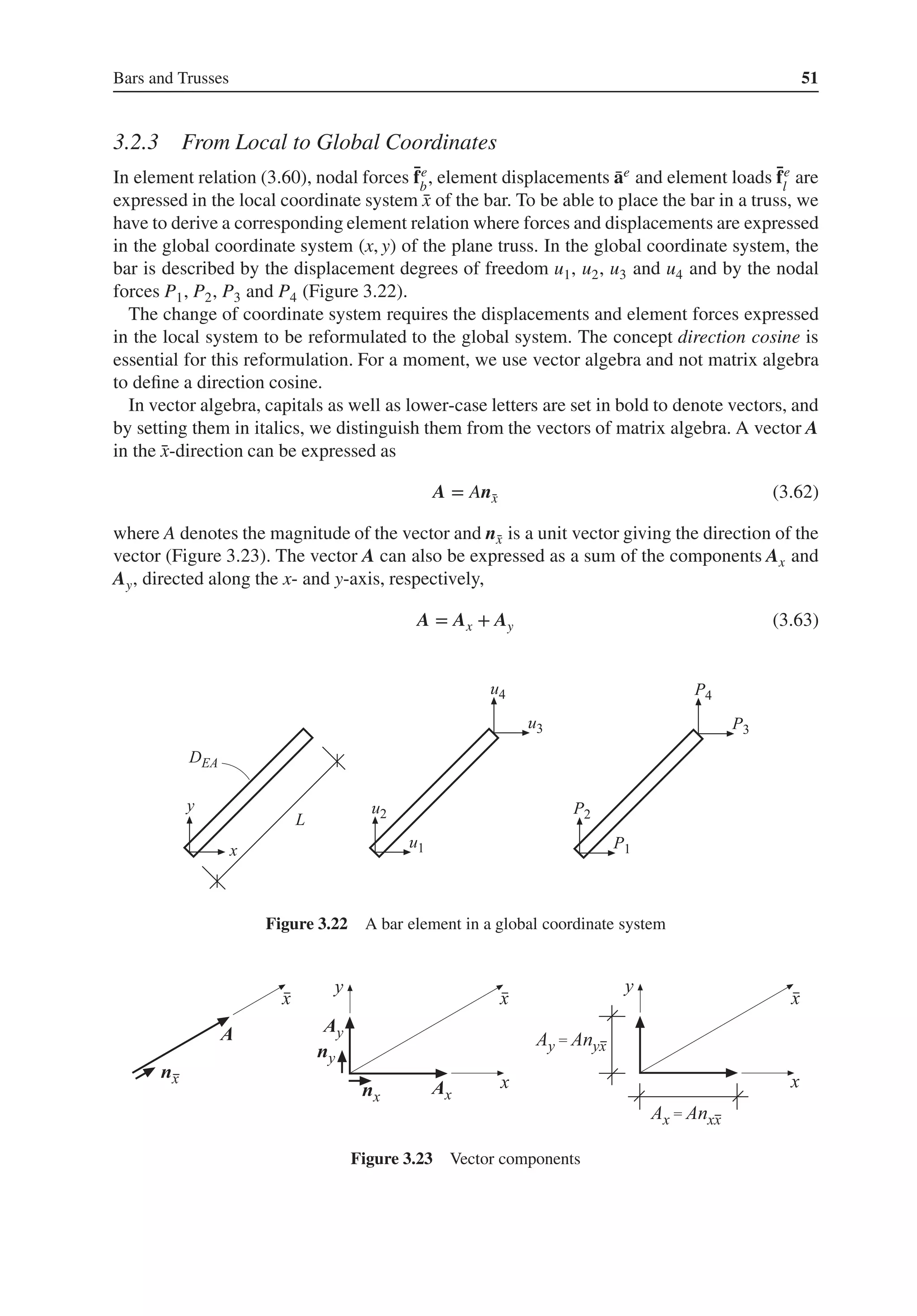
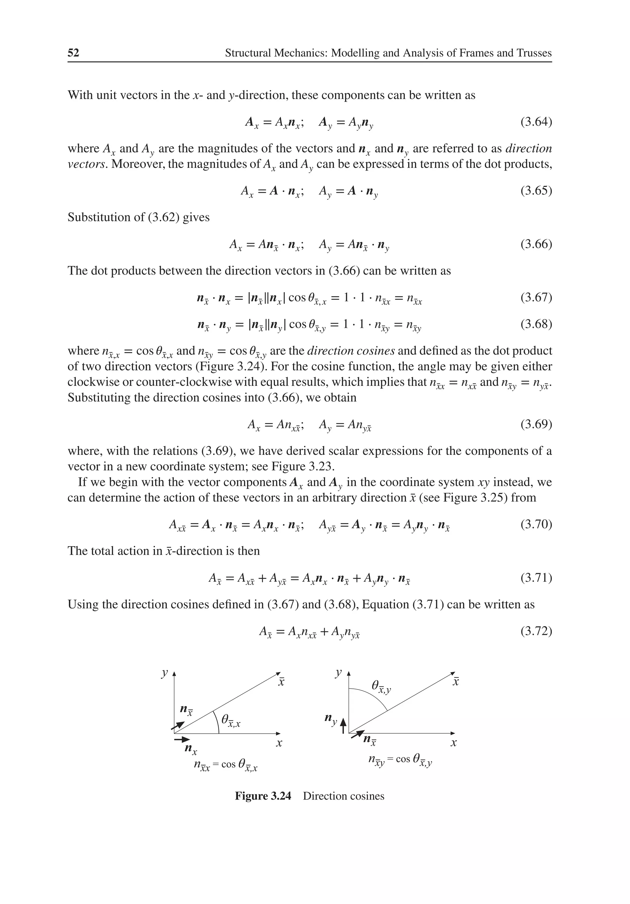
![Bars and Trusses 53
Figure 3.25 Total vector action in the ̄
x-direction
The scalar relations (3.69) and (3.72) will be used for the transformations between different
coordinate systems.
With relation (3.72), the displacements ̄
u1 and ̄
u2 in the longitudinal direction of the bar can
be expressed in the global displacement degrees of freedom u1, u2, u3 and u4
̄
u1 = nx̄
xu1 + nȳ
xu2 (3.73)
̄
u2 = nx̄
xu3 + nȳ
xu4 (3.74)
or in matrix form
̄
ae
= Gae
(3.75)
where
̄
ae
=
[
̄
u1
̄
u2
]
; G =
[
nx̄
x nȳ
x 0 0
0 0 nx̄
x nȳ
x
]
; ae
=
⎡
⎢
⎢
⎢
⎣
u1
u2
u3
u4
⎤
⎥
⎥
⎥
⎦
(3.76)
Using the relations (3.69), the components P1, P2, P3 and P4 of the nodal forces ̄
P1 and ̄
P2
can be expressed as
P1 = nx̄
x
̄
P1 (3.77)
P2 = nȳ
x
̄
P1 (3.78)
P3 = nx̄
x
̄
P2 (3.79)
P4 = nȳ
x
̄
P2 (3.80)
or in matrix form
fe
b = GT ̄
fe
b (3.81)
where
fe
b =
⎡
⎢
⎢
⎢
⎣
P1
P2
P3
P4
⎤
⎥
⎥
⎥
⎦
; GT
=
⎡
⎢
⎢
⎢
⎣
nx̄
x 0
nȳ
x 0
0 nx̄
x
0 nȳ
x
⎤
⎥
⎥
⎥
⎦
; ̄
fe
b =
[
̄
P1
̄
P2
]
(3.82)](https://image.slidesharecdn.com/structuralmechanicsmodellingandanalysisofframesandtrussespdfdrive-230720064114-5e1f9a93/75/Structural-mechanics-_-modelling-and-analysis-of-frames-and-trusses-PDFDrive-pdf-67-2048.jpg)
![54 Structural Mechanics: Modelling and Analysis of Frames and Trusses
In the same manner, a relation between the equivalent element loads fe
l
in a global system and
the equivalent element loads ̄
fe
l
in a local system can be written as
fe
l = GT ̄
fe
l (3.83)
where
fe
l =
⎡
⎢
⎢
⎢
⎢
⎣
fe
l1
fe
l2
fe
l3
fe
l4
⎤
⎥
⎥
⎥
⎥
⎦
(3.84)
The matrices G and GT are referred to as transformation matrices and their purpose is to
transform quantities so that they can be expressed in different coordinatesystems. The contents
of a transformation matrix depend on the type of quantity/quantities to be transformed and
between which coordinate systems the transformation is performed.
If we substitute the transformations (3.81), (3.75) and (3.83) into the element relation (3.58),
we get a new element relation, one with its quantities expressed in the directions of the global
coordinate system,
Ke
ae
= fe
(3.85)
where
Ke
= GT ̄
Ke
G; fe
= fe
b + fe
l (3.86)
Figure 3.26 shows how transformations of displacements and forces between different coor-
dinate systems lead to a relation for the bar element in global coordinates.
If the matrix multiplication in Equation (3.86) is performed, we obtain the element stiffness
matrix Ke for a bar element in the global system as
Ke
=
DEA
L
[
C −C
−C C
]
; C =
[
nx̄
xnx̄
x nx̄
xnȳ
x
nȳ
xnx̄
x nȳ
xnȳ
x
]
(3.87)
fe
b
= GT ̄
fe
b
(3.81)
fe
l
= GT ̄
fe
l
(3.83)
̄
Ke
̄
ae
= ̄
fe
(3.60)
̄
fe
= ̄
fe
b
+ ̄
fe
l
(3.61)
̄
ae
= Gae
(3.75)
⎫
⎪
⎪
⎪
⎬
⎪
⎪
⎪
⎭
⇒ Ke
ae
= fe
(3.85)
where
Ke
= GT ̄
Ke
G; fe
= fe
b
+ fe
l
Figure 3.26 From local coordinates to global coordinates](https://image.slidesharecdn.com/structuralmechanicsmodellingandanalysisofframesandtrussespdfdrive-230720064114-5e1f9a93/75/Structural-mechanics-_-modelling-and-analysis-of-frames-and-trusses-PDFDrive-pdf-68-2048.jpg)
![Bars and Trusses 63
the boundary condition matrix
boundary conditions =
⎡
⎢
⎢
⎢
⎢
⎢
⎢
⎣
1 0
2 0
3 0
4 0
7 0
8 0
⎤
⎥
⎥
⎥
⎥
⎥
⎥
⎦
(22)
The only degrees of freedom where the displacement is not prescribed are a5 and a6. In the
degrees of freedom where the displacement is prescribed, support forces arise. These are
at present unknown and denoted as fb,1, fb,2, fb,3, fb,4, fb,7 and fb,8. The displacement vector
a and the boundary force vector fb can with that be written as
a =
⎡
⎢
⎢
⎢
⎢
⎢
⎢
⎢
⎢
⎣
0
0
0
0
a5
a6
0
0
⎤
⎥
⎥
⎥
⎥
⎥
⎥
⎥
⎥
⎦
; fb =
⎡
⎢
⎢
⎢
⎢
⎢
⎢
⎢
⎢
⎣
fb,1
fb,2
fb,3
fb,4
0
0
fb,7
fb,8
⎤
⎥
⎥
⎥
⎥
⎥
⎥
⎥
⎥
⎦
(23)
Solving the system of equations
We can now establish a system of equations Ka = fl + fb for the truss,
106
⎡
⎢
⎢
⎢
⎢
⎢
⎢
⎢
⎢
⎣
75 0 0 0 −75 0 0 0
0 0 0 0 0 0 0 0
0 0 64 −48 −64 48 0 0
0 0 −48 36 48 −36 0 0
−75 0 −64 48 139 −48 0 0
0 0 48 −36 −48 86 0 −50
0 0 0 0 0 0 0 0
0 0 0 0 0 −50 0 50
⎤
⎥
⎥
⎥
⎥
⎥
⎥
⎥
⎥
⎦
⎡
⎢
⎢
⎢
⎢
⎢
⎢
⎢
⎢
⎣
0
0
0
0
a5
a6
0
0
⎤
⎥
⎥
⎥
⎥
⎥
⎥
⎥
⎥
⎦
=
⎡
⎢
⎢
⎢
⎢
⎢
⎢
⎢
⎢
⎣
0
0
0
0
0
−80
0
0
⎤
⎥
⎥
⎥
⎥
⎥
⎥
⎥
⎥
⎦
103
+
⎡
⎢
⎢
⎢
⎢
⎢
⎢
⎢
⎢
⎣
fb,1
fb,2
fb,3
fb,4
0
0
fb,7
fb,8
⎤
⎥
⎥
⎥
⎥
⎥
⎥
⎥
⎥
⎦
(24)
The system of equations contains eight equations and eight unknowns; the displacements
a5 and a6 and the support forces fb,1, fb,2, fb,3, fb,4, fb,7 and fb,8. Considering the prescribed
displacements, the system of equations can be reduced to
106
[
139 −48
−48 86
]
[
a5
a6
]
=
[
0
−80
]
103
(25)
and the displacements a5 and a6 be determined
[
a5
a6
]
=
[
−0.3979
−1.1523
]
10−3
(26)](https://image.slidesharecdn.com/structuralmechanicsmodellingandanalysisofframesandtrussespdfdrive-230720064114-5e1f9a93/75/Structural-mechanics-_-modelling-and-analysis-of-frames-and-trusses-PDFDrive-pdf-77-2048.jpg)
![64 Structural Mechanics: Modelling and Analysis of Frames and Trusses
This means that the free node is displaced 0.40 mm leftwards and 1.15 mm downwards.
The displacements are shown in Figure 3.
Figure 3 The computed displacements drawn in a magnified scale
When a5 and a6 have been determined, all nodal displacements are known and the sup-
port forces fb,1, fb,2, fb,3, fb,4, fb,7 and fb,8 can be determined from the global system of
equations,
⎡
⎢
⎢
⎢
⎢
⎢
⎢
⎣
fb,1
fb,2
fb,3
fb,4
fb,7
fb,8
⎤
⎥
⎥
⎥
⎥
⎥
⎥
⎦
= 106
⎡
⎢
⎢
⎢
⎢
⎢
⎢
⎣
−75 0
0 0
−64 48
48 −36
0 0
0 −50
⎤
⎥
⎥
⎥
⎥
⎥
⎥
⎦
[
a5
a6
]
=
⎡
⎢
⎢
⎢
⎢
⎢
⎢
⎣
29.84
0
−29.84
22.38
0
57.62
⎤
⎥
⎥
⎥
⎥
⎥
⎥
⎦
103
(27)
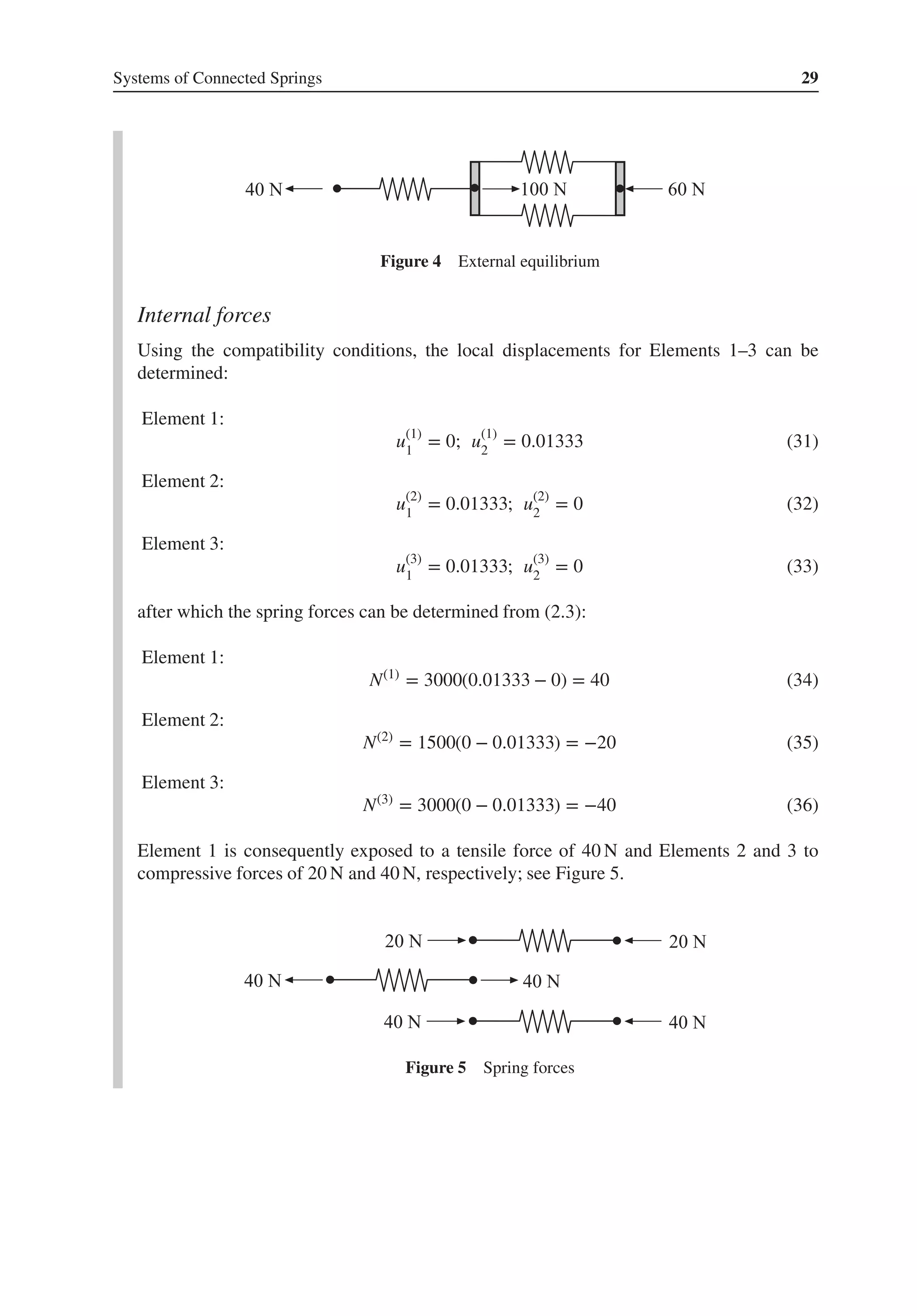
The external load and the support forces computed are shown in Figure 4. We can conclude
that the sum of the horizontal forces as well as the sum of vertical forces is zero. Conse-
quently, equilibria of external forces are fulfilled. By establishing an equation of moments,
we can also show that the equilibrium of moments is fulfilled.
Figure 4 The external load and the computed support forces](https://image.slidesharecdn.com/structuralmechanicsmodellingandanalysisofframesandtrussespdfdrive-230720064114-5e1f9a93/75/Structural-mechanics-_-modelling-and-analysis-of-frames-and-trusses-PDFDrive-pdf-78-2048.jpg)
![Bars and Trusses 65
Compute internal forces
Beginning from the compatibility relations, the displacements for Element 1 can be
determined
a1
=
⎡
⎢
⎢
⎢
⎣
0
0
−0.3979
−1.1523
⎤
⎥
⎥
⎥
⎦
10−3
(28)
Furthermore, using (3.75), the displacements can be expressed in the local coordinate sys-
tem of the element
̄
a1
= Ga1
=
[
1 0 0 0
0 0 1 0
]⎡
⎢
⎢
⎢
⎣
0
0
−0.3979
−1.1523
⎤
⎥
⎥
⎥
⎦
10−3
=
[
0
−0.3979
]
10−3
(29)
and the normal force in the element can be computed from (3.52)
N(1)
= EA1B̄
a1
= 200.0 × 109
⋅ 6.0 × 10−4 1
1.6
[
−1 1
]
[
0
−0.3979
]
10−3
= −29.84 × 10³
(30)
For Element 2, we have in the same manner:
a2
=
⎡
⎢
⎢
⎢
⎣
−0.3979
−1.1523
0
0
⎤
⎥
⎥
⎥
⎦
10−3
(31)
̄
a2
= Ga2
=
[
0 1 0 0
0 0 0 1
]⎡
⎢
⎢
⎢
⎣
−0.3979
−1.1523
0
0
⎤
⎥
⎥
⎥
⎦
10−3
=
[
−1.1523
0
]
10−3
(32)
N(2)
= EA2B̄
a2
= 200.0 × 109
⋅ 3.0 × 10−4 1
1.2
[
−1 1
]
[
−1.1523
0
]
10−3
= 57.62 × 10³
(33)
and for Element 3
a3
=
⎡
⎢
⎢
⎢
⎣
0
0
−0.3979
−1.1523
⎤
⎥
⎥
⎥
⎦
10−3
(34)](https://image.slidesharecdn.com/structuralmechanicsmodellingandanalysisofframesandtrussespdfdrive-230720064114-5e1f9a93/75/Structural-mechanics-_-modelling-and-analysis-of-frames-and-trusses-PDFDrive-pdf-79-2048.jpg)
![66 Structural Mechanics: Modelling and Analysis of Frames and Trusses
̄
a3
= Ga3
=
[
0.8 −0.6 0 0
0 0 0.8 −0.6
] ⎡
⎢
⎢
⎢
⎣
0
0
−0.3979
−1.1523
⎤
⎥
⎥
⎥
⎦
10−3
=
[
0
0.3730
]
10−3
(35)
N(3)
= EA3B̄
a3
= 200.0 × 109
⋅ 10.0 × 10−4 1
2.0
[
−1 1
]
[
0
0.3730
]
10−3
= 37.30 × 10³
(36)
This result means that the normal forces in the three elements are −29.84 kN, 57.62 kN
and 37.30 kN, respectively; see Figure 5.
Figure 5 The normal forces in the bars
Exercises
3.1 . ( ) ( ) ( )
ϕ](https://image.slidesharecdn.com/structuralmechanicsmodellingandanalysisofframesandtrussespdfdrive-230720064114-5e1f9a93/75/Structural-mechanics-_-modelling-and-analysis-of-frames-and-trusses-PDFDrive-pdf-80-2048.jpg)

![82 Structural Mechanics: Modelling and Analysis of Frames and Trusses
We first seek a form of the solution of the homogeneous equation written as a function of the
displacements ̄
u1, ̄
u2, ̄
u3 and ̄
u4.
If the homogeneous differential equation (4.29) is divided by the stiffness DEI, we obtain
d4𝑣
d̄
x4
= 0 (4.31)
Integrating four times gives
𝑣h(̄
x) = 𝛼1 + 𝛼2̄
x + 𝛼3̄
x2
+ 𝛼4 ̄
x3
(4.32)
or in matrix form
𝑣h(̄
x) = ̄
N𝛂 (4.33)
where ̄
N = ̄
N(̄
x) describes how the solution varies along the ̄
x-axis and 𝛂 contains the constants
of integration,
̄
N =
[
1 ̄
x ̄
x2 ̄
x3
]
; 𝛂 =
⎡
⎢
⎢
⎢
⎣
𝛼1
𝛼2
𝛼3
𝛼4
⎤
⎥
⎥
⎥
⎦
(4.34)
At the nodes of the beam, at ̄
x = 0 and ̄
x = L, we have the boundary conditions
𝑣h(0) = ̄
u1 (4.35)
(
d𝑣h
d̄
x
)
̄
x=0
= ̄
u2 (4.36)
𝑣h(L) = ̄
u3 (4.37)
(
d𝑣h
d̄
x
)
̄
x=L
= ̄
u4 (4.38)
Substitution of these conditions into (4.33) gives
̄
u1 = 𝛼1 (4.39)
̄
u2 = 𝛼2 (4.40)
̄
u3 = 𝛼1 + 𝛼2L + 𝛼3L2
+ 𝛼4L3
(4.41)
̄
u4 = 𝛼2 + 2𝛼3L + 3𝛼4L2
(4.42)
or in matrix form
̄
ae
= C𝛂 (4.43)
where
̄
ae
=
⎡
⎢
⎢
⎢
⎣
̄
u1
̄
u2
̄
u3
̄
u4
⎤
⎥
⎥
⎥
⎦
; C =
⎡
⎢
⎢
⎢
⎣
1 0 0 0
0 1 0 0
1 L L2 L3
0 1 2L 3L2
⎤
⎥
⎥
⎥
⎦
(4.44)](https://image.slidesharecdn.com/structuralmechanicsmodellingandanalysisofframesandtrussespdfdrive-230720064114-5e1f9a93/75/Structural-mechanics-_-modelling-and-analysis-of-frames-and-trusses-PDFDrive-pdf-96-2048.jpg)
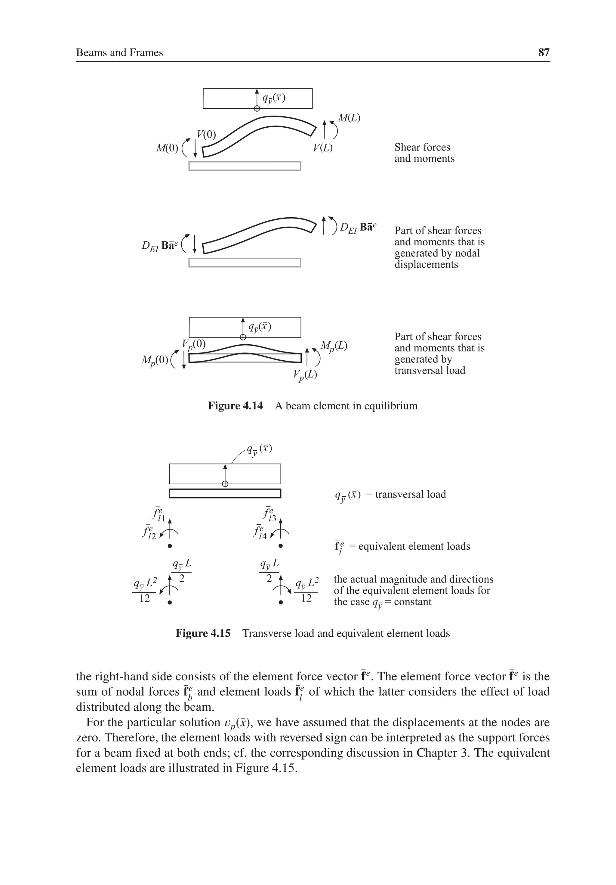
![Beams and Frames 83
By inverting C, we can express the constants of integration𝛂 as a functions of the displacement
degrees of freedom of the element ̄
ae,
𝛂 = C−1
̄
ae
(4.45)
where
C−1
=
⎡
⎢
⎢
⎢
⎢
⎢
⎣
1 0 0 0
0 1 0 0
− 3
L2 −2
L
3
L2 −1
L
2
L3
1
L2 − 2
L3
1
L2
⎤
⎥
⎥
⎥
⎥
⎥
⎦
(4.46)
Substituting (4.45) into (4.33), we obtain the solution 𝑣h(̄
x) as
𝑣h(̄
x) = N̄
ae
(4.47)
where
N = ̄
NC−1
=
[
1 ̄
x ̄
x2 ̄
x3
]
⎡
⎢
⎢
⎢
⎢
⎢
⎣
1 0 0 0
0 1 0 0
− 3
L2 −2
L
3
L2 −1
L
2
L3
1
L2 − 2
L3
1
L2
⎤
⎥
⎥
⎥
⎥
⎥
⎦
(4.48)
which gives
N =
[
1 − 3 ̄
x2
L2 + 2 ̄
x3
L3 ̄
x − 2 ̄
x2
L
+ ̄
x3
L2 3 ̄
x2
L2 − 2 ̄
x3
L3 − ̄
x2
L
+ ̄
x3
L2
]
(4.49)
With that, we have reformulated 𝑣h(̄
x) written as a general polynomial (4.32) to a solution in
the form
𝑣h(̄
x) = N̄
ae
= N1(̄
x) ̄
u1 + N2(̄
x) ̄
u2 + N3(̄
x) ̄
u3 + N4(̄
x) ̄
u4 (4.50)
where
N1(̄
x) = 1 − 3
̄
x2
L2
+ 2
̄
x3
L3
(4.51)
N2(̄
x) = ̄
x − 2
̄
x2
L
+
̄
x3
L2
(4.52)
N3(̄
x) = 3
̄
x2
L2
− 2
̄
x3
L3
(4.53)
N4(̄
x) = −
̄
x2
L
+
̄
x3
L2
(4.54)
The functions N1(̄
x)–N4(̄
x) describe how the solution varies with ̄
x and are referred to as base
functions or shape functions; cf. Chapter 3. We have in (4.50) an expression where the product
Ni(̄
x) ̄
ui gives the contributionto 𝑣h(̄
x) from the displacement ̄
ui and where Ni(̄
x) states its shape
and ̄
ui its size. Substitution of (4.47) into the general solution of the differential equation (4.30)
gives
𝑣(̄
x) = N̄
ae
+ 𝑣p(̄
x) (4.55)](https://image.slidesharecdn.com/structuralmechanicsmodellingandanalysisofframesandtrussespdfdrive-230720064114-5e1f9a93/75/Structural-mechanics-_-modelling-and-analysis-of-frames-and-trusses-PDFDrive-pdf-97-2048.jpg)
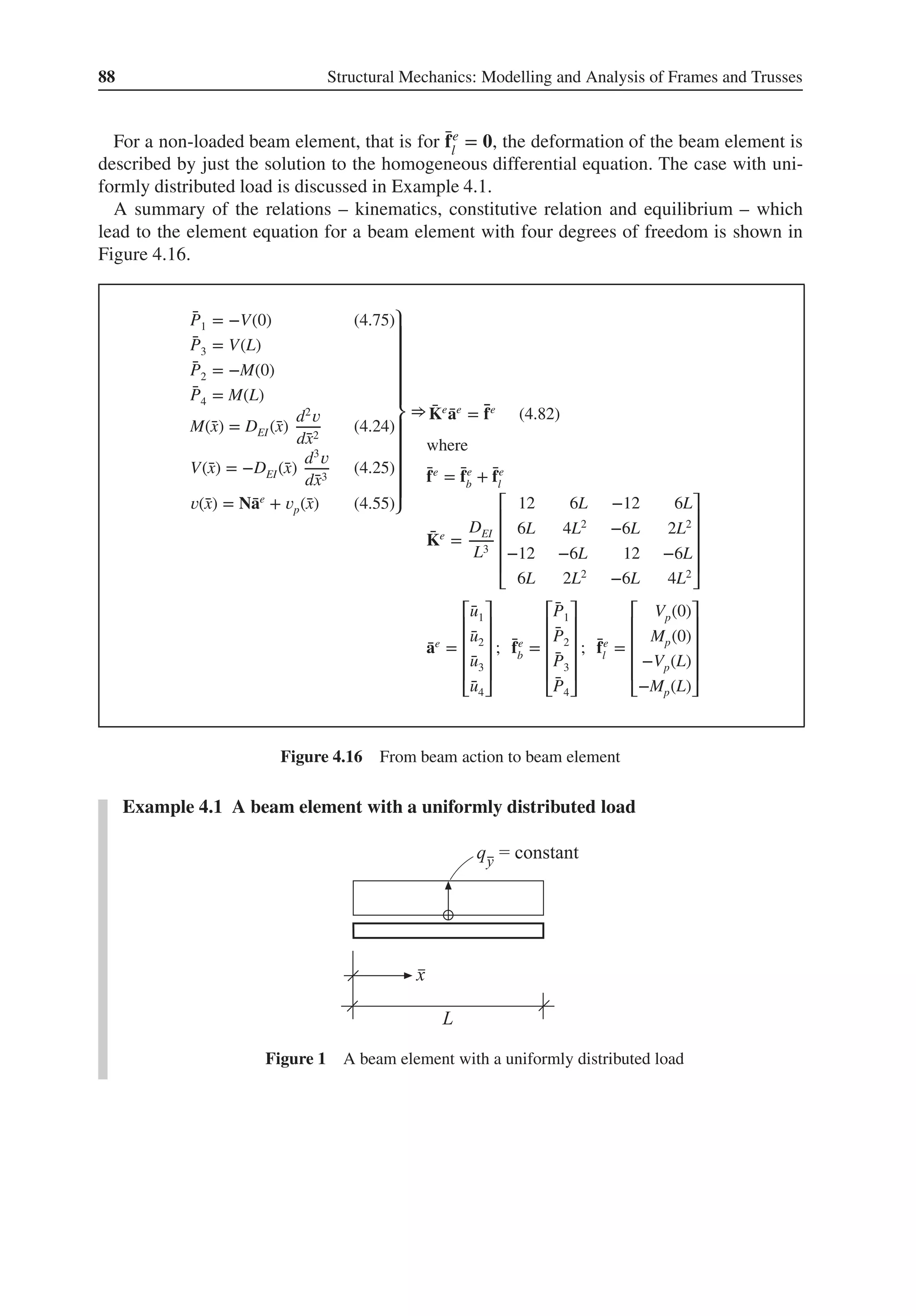
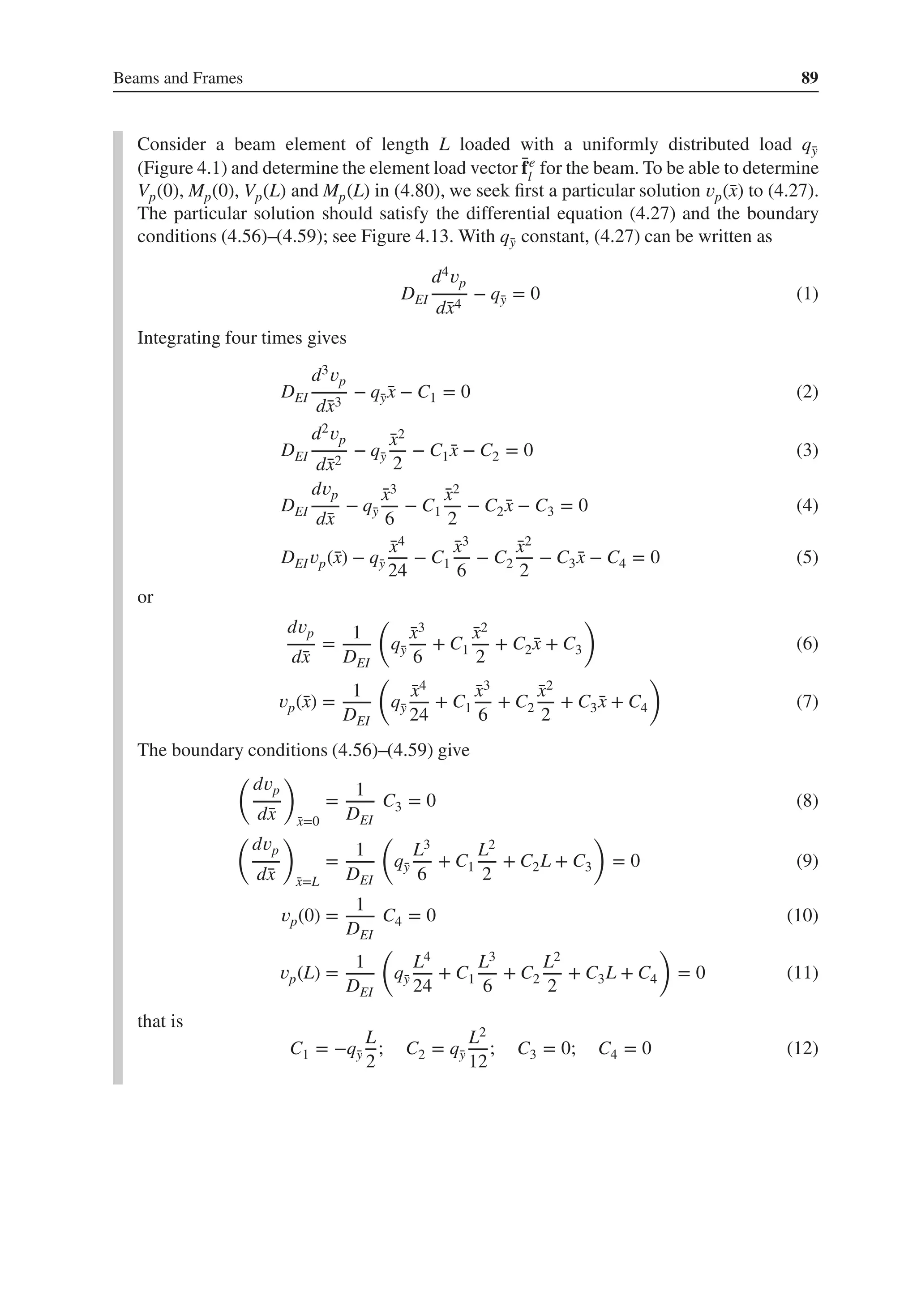
![Beams and Frames 85
Differentiating (4.55) three times gives
d𝑣
d̄
x
=
dN
d̄
x
̄
ae
+
d𝑣p
d̄
x
(4.60)
d2𝑣
d̄
x2
= B̄
ae
+
d2𝑣p
d̄
x2
(4.61)
d3𝑣
d̄
x3
=
dB
d̄
x
̄
ae
+
d3𝑣p
d̄
x3
(4.62)
where
dN
d̄
x
=
d ̄
N
d̄
x
C−1
=
[
0 1 2̄
x 3̄
x2
]
⎡
⎢
⎢
⎢
⎢
⎢
⎣
1 0 0 0
0 1 0 0
− 3
L2 −2
L
3
L2 −1
L
2
L3
1
L2 − 2
L3
1
L2
⎤
⎥
⎥
⎥
⎥
⎥
⎦
(4.63)
B =
d2N
d̄
x2
=
d2 ̄
N
d̄
x2
C−1
=
[
0 0 2 6̄
x
]
⎡
⎢
⎢
⎢
⎢
⎢
⎣
1 0 0 0
0 1 0 0
− 3
L2 −2
L
3
L2 −1
L
2
L3
1
L2 − 2
L3
1
L2
⎤
⎥
⎥
⎥
⎥
⎥
⎦
(4.64)
dB
d̄
x
=
d3N
d̄
x3
=
d3 ̄
N
d̄
x3
C−1
=
[
0 0 0 6
]
⎡
⎢
⎢
⎢
⎢
⎢
⎣
1 0 0 0
0 1 0 0
− 3
L2 −2
L
3
L2 −1
L
2
L3
1
L2 − 2
L3
1
L2
⎤
⎥
⎥
⎥
⎥
⎥
⎦
(4.65)
which gives
dN
d̄
x
=
[
−6 ̄
x
L2 + 6 ̄
x2
L3 1 − 4 ̄
x
L
+ 3 ̄
x2
L2 6 ̄
x
L2 − 6 ̄
x2
L3 −2 ̄
x
L
+ 3 ̄
x2
L2
]
(4.66)
B =
[
− 6
L2 + 12 ̄
x
L3 −4
L
+ 6 ̄
x
L2
6
L2 − 12 ̄
x
L3 −2
L
+ 6 ̄
x
L2
]
(4.67)
dB
d̄
x
=
[
12
L3
6
L2 −12
L3
6
L2
]
(4.68)
Substituting (4.55) into (4.24) and (4.22), we obtain expressions for moments and shear forces
as functions of the displacements of the nodes,
M(̄
x) = DEI
(
B̄
ae
+
d2𝑣p
d̄
x2
)
(4.69)
V(̄
x) = −
dM
d̄
x
= −DEI
(
dB
d̄
x
̄
ae
+
d3𝑣p
d̄
x3
)
(4.70)](https://image.slidesharecdn.com/structuralmechanicsmodellingandanalysisofframesandtrussespdfdrive-230720064114-5e1f9a93/75/Structural-mechanics-_-modelling-and-analysis-of-frames-and-trusses-PDFDrive-pdf-99-2048.jpg)
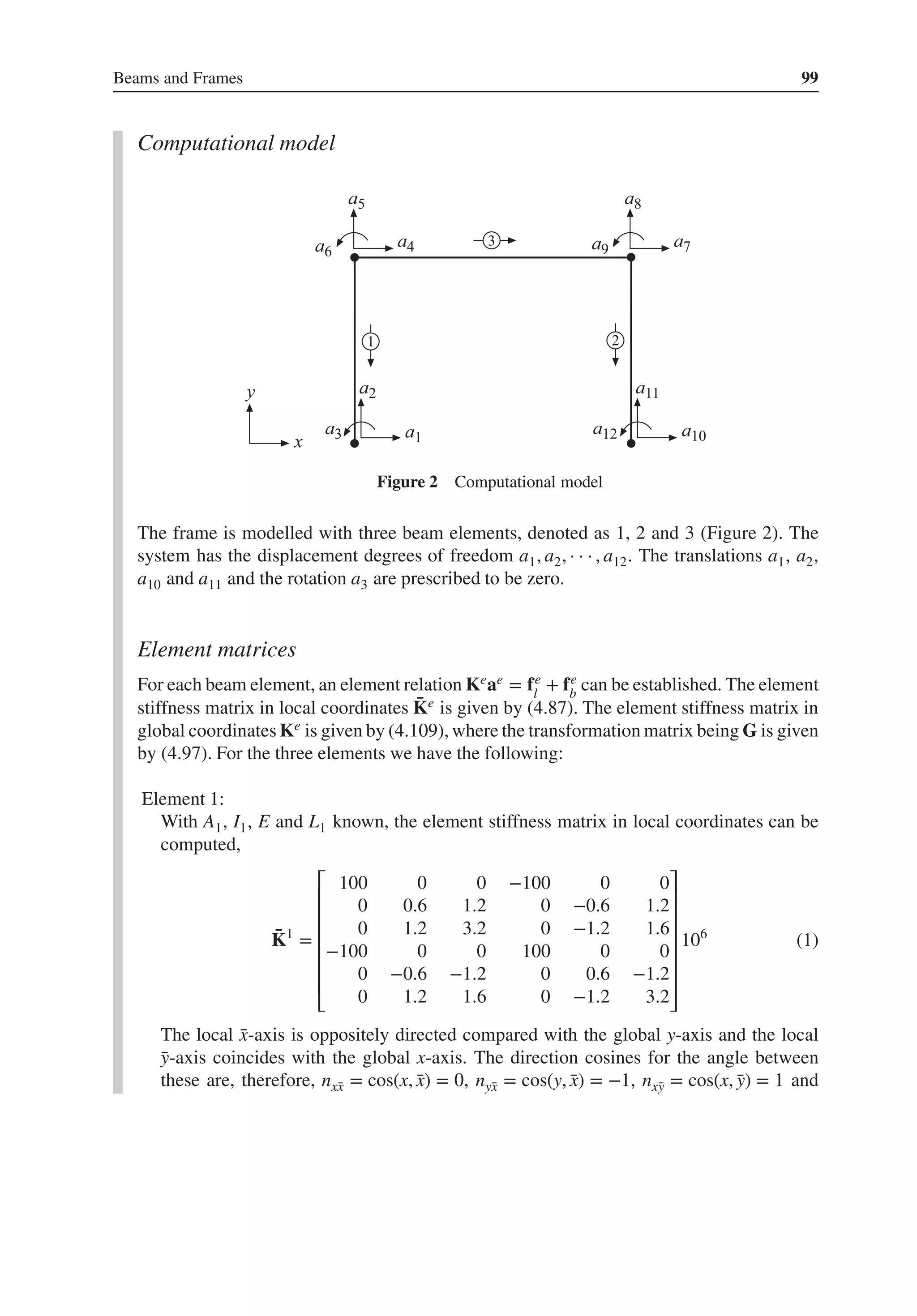
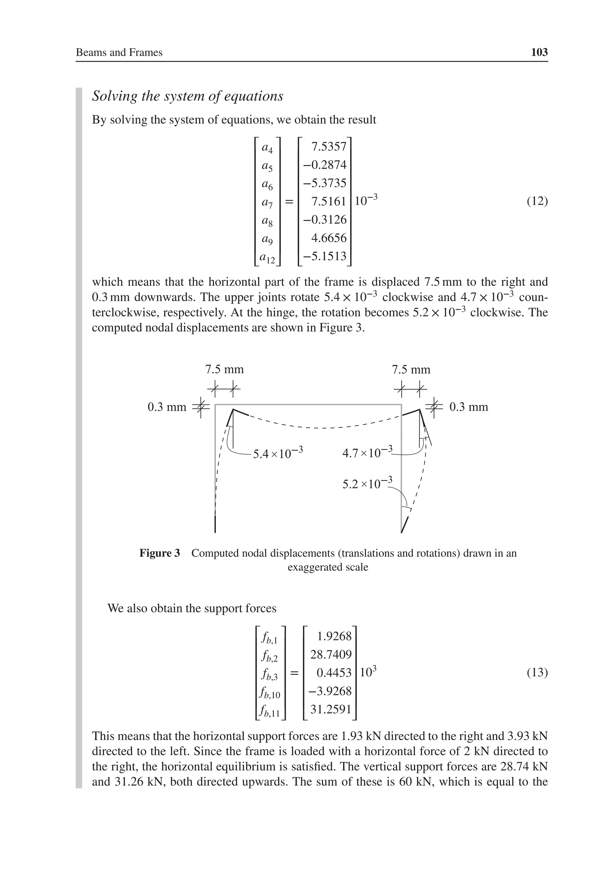
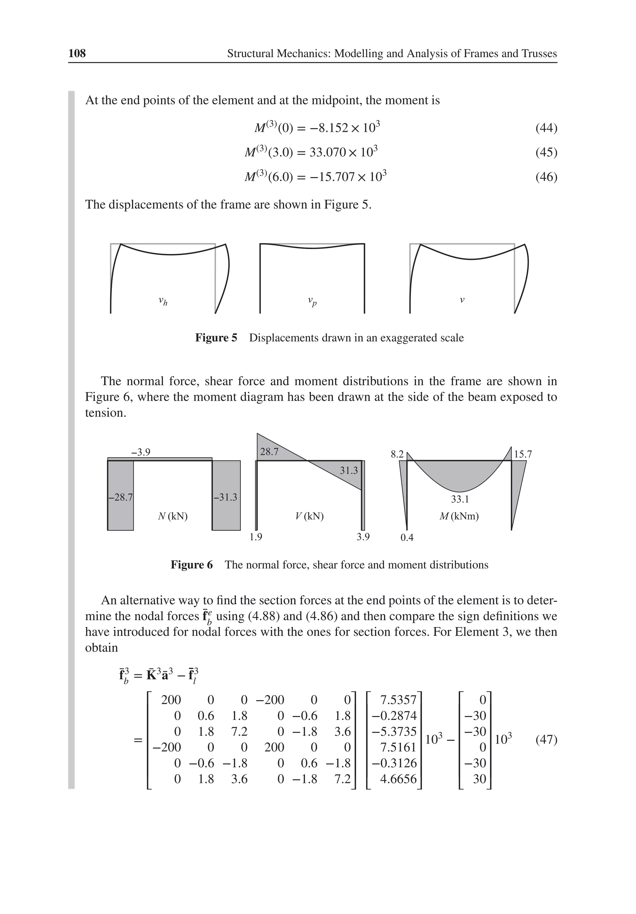
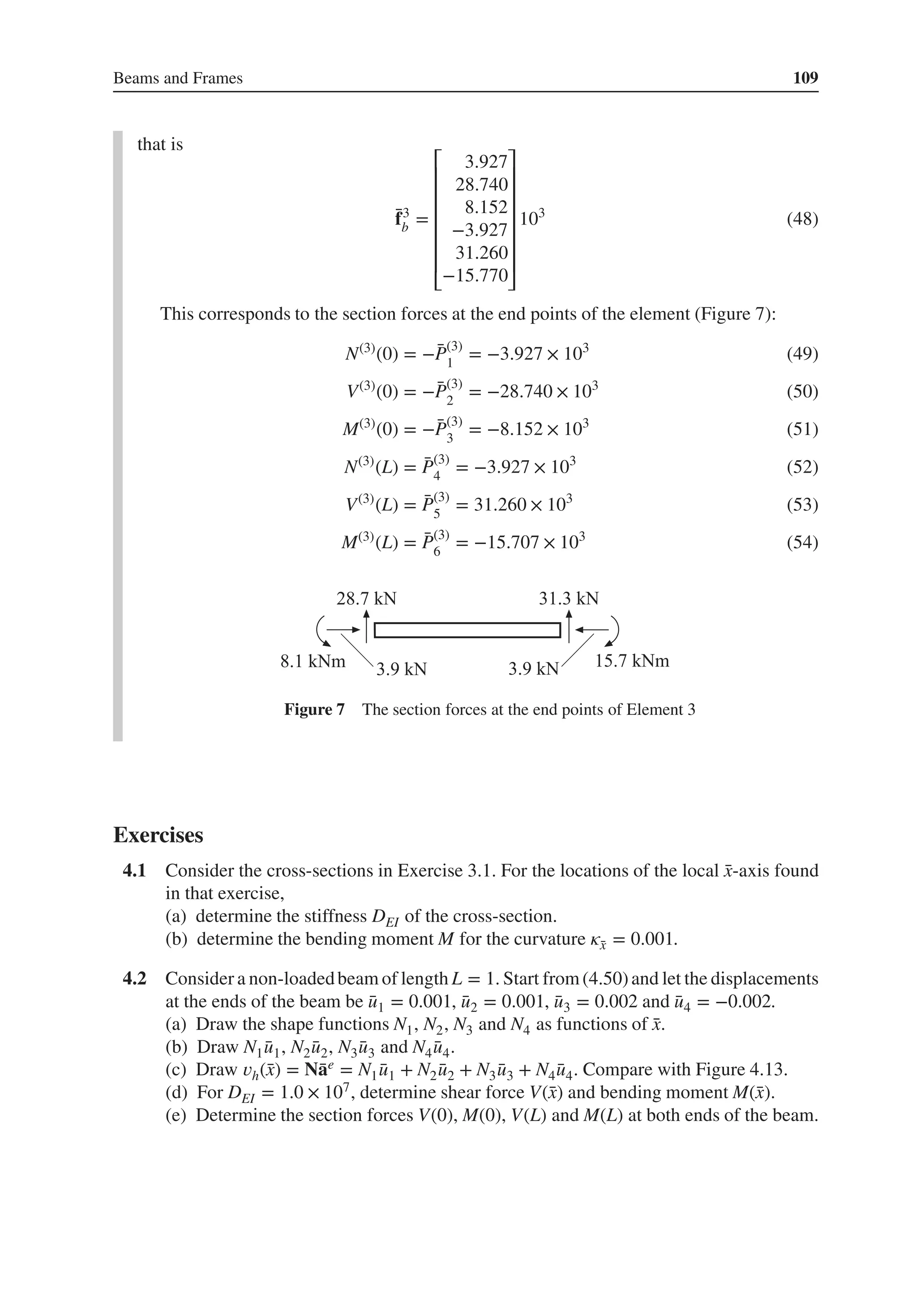
![104 Structural Mechanics: Modelling and Analysis of Frames and Trusses
distributed load on Element 3. By establishing a moment equation, we can also conclude
that the external moment equilibrium is satisfied. Figure 4 shows the external load and the
computed support forces.
Figure 4 External load and computed support forces
Displacements and internal forces
With the global node displacements a known, we can, with use of compatibility relations,
find the node displacements for each element. After that, the node displacements for each
element can be transformed to local coordinates using (4.96).
For Element 1, we obtain
̄
a1
= G1
a1
=
⎡
⎢
⎢
⎢
⎢
⎢
⎢
⎣
0 −1 0 0 0 0
1 0 0 0 0 0
0 0 1 0 0 0
0 0 0 0 −1 0
0 0 0 1 0 0
0 0 0 0 0 1
⎤
⎥
⎥
⎥
⎥
⎥
⎥
⎦
⎡
⎢
⎢
⎢
⎢
⎢
⎢
⎣
7.5357
−0.2874
−5.3735
0
0
0
⎤
⎥
⎥
⎥
⎥
⎥
⎥
⎦
10−3
=
⎡
⎢
⎢
⎢
⎢
⎢
⎢
⎣
0.2874
7.5357
−5.3735
0
0
0
⎤
⎥
⎥
⎥
⎥
⎥
⎥
⎦
10−3
(14)
The axial and the transversal displacements along the element are determined by (3.46) and
(4.55) giving
u(1)
(̄
x) =
[
1 −
̄
x
4.0
̄
x
4.0
]
[
0.2874
0
]
10−3
= (0.2874 − 0.0718̄
x) × 10−3
(15)](https://image.slidesharecdn.com/structuralmechanicsmodellingandanalysisofframesandtrussespdfdrive-230720064114-5e1f9a93/75/Structural-mechanics-_-modelling-and-analysis-of-frames-and-trusses-PDFDrive-pdf-118-2048.jpg)
![Beams and Frames 105
𝑣(1)
(̄
x) =
⎡
⎢
⎢
⎢
⎢
⎢
⎢
⎣
1 − 3 ̄
x2
4.02 + 2 ̄
x3
4.03
̄
x − 2 ̄
x2
4.0
+ ̄
x3
4.02
3 ̄
x2
4.02 − 2 ̄
x3
4.03
− ̄
x2
4.0
+ ̄
x3
4.02
⎤
⎥
⎥
⎥
⎥
⎥
⎥
⎦
T
⎡
⎢
⎢
⎢
⎢
⎣
7.5357
−5.3735
0
0
⎤
⎥
⎥
⎥
⎥
⎦
10−3
= (7.5357 − 5.3735̄
x + 1.2738̄
x2
− 0.1004̄
x3
) × 10−3
(16)
Next, we compute the section forces along the beam. For the normal force, we substitute
the displacements directed along the element into (3.52). For Element 1, we then obtain
N(1)
= 400.0 × 10⁶
[
− 1
4.0
1
4.0
][
0.2874
0
]
10−3
= −28.740 × 10³
(17)
For the moment and the shear force, we substitute the displacements directed perpendicular
to the element and the rotations into (4.71) and (4.72), respectively.Since no load acts along
the element, Mp(̄
x) = 0 and Vp(̄
x) = 0, we obtain
V(1)
= −3.2 × 10⁶
⎡
⎢
⎢
⎢
⎢
⎢
⎢
⎣
12
4.03
6
4.02
− 12
4.03
6
4.02
⎤
⎥
⎥
⎥
⎥
⎥
⎥
⎦
T
⎡
⎢
⎢
⎢
⎢
⎢
⎢
⎣
7.5357
−5.3735
0
0
⎤
⎥
⎥
⎥
⎥
⎥
⎥
⎦
10−3
= 1.927 × 10³
(18)
M(1)
(̄
x) = 3.2 × 10⁶
⎡
⎢
⎢
⎢
⎢
⎢
⎢
⎣
− 6
4.02 + 12 ̄
x
4.03
− 4
4.0
+ 6 ̄
x
4.02
6
4.02 − 12 ̄
x
4.03
− 2
4.0
+ 6 ̄
x
4.02
⎤
⎥
⎥
⎥
⎥
⎥
⎥
⎦
T
⎡
⎢
⎢
⎢
⎢
⎢
⎢
⎣
7.5357
−5.3735
0
0
⎤
⎥
⎥
⎥
⎥
⎥
⎥
⎦
10−3
= (8.152 − 1.927̄
x) × 103
(19)
At the end points of the element, the moment is
M(1)
(0) = 8.152 × 10³
(20)
M(1)
(4.0) = 0.445 × 10³
(21)
For Element 2, we obtain
̄
a2
= G2
a2
=
⎡
⎢
⎢
⎢
⎢
⎢
⎢
⎣
0 −1 0 0 0 0
1 0 0 0 0 0
0 0 1 0 0 0
0 0 0 0 −1 0
0 0 0 1 0 0
0 0 0 0 0 1
⎤
⎥
⎥
⎥
⎥
⎥
⎥
⎦
⎡
⎢
⎢
⎢
⎢
⎢
⎢
⎣
7.5161
−0.3126
4.6656
0
0
−5.1513
⎤
⎥
⎥
⎥
⎥
⎥
⎥
⎦
10−3
=
⎡
⎢
⎢
⎢
⎢
⎢
⎢
⎣
0.3126
7.5161
4.6656
0
0
−5.1513
⎤
⎥
⎥
⎥
⎥
⎥
⎥
⎦
10−3
(22)](https://image.slidesharecdn.com/structuralmechanicsmodellingandanalysisofframesandtrussespdfdrive-230720064114-5e1f9a93/75/Structural-mechanics-_-modelling-and-analysis-of-frames-and-trusses-PDFDrive-pdf-119-2048.jpg)
![106 Structural Mechanics: Modelling and Analysis of Frames and Trusses
u(2)
(̄
x) =
[
1 − ̄
x
4.0
̄
x
4.0
] [
0.3126
0
]
10−3
= (0.3126 − 0.0782̄
x) × 10−3
(23)
𝑣(2)
(̄
x) =
⎡
⎢
⎢
⎢
⎢
⎢
⎢
⎣
1 − 3 ̄
x2
4.02 + 2 ̄
x3
4.03
̄
x − 2 ̄
x2
4.0
+ ̄
x3
4.02
3 ̄
x2
4.02 − 2 ̄
x3
4.03
− ̄
x2
4.0
+ ̄
x3
4.02
⎤
⎥
⎥
⎥
⎥
⎥
⎥
⎦
T
⎡
⎢
⎢
⎢
⎣
7.5161
4.6656
0
−5.1513
⎤
⎥
⎥
⎥
⎦
10−3
= (7.5161 + 4.6656̄
x − 2.4542̄
x2
+ 0.2045̄
x3
) × 10−3
(24)
N(2)
= 400.0 × 10⁶
[
− 1
4.0
1
4.0
] [
0.3126
0
]
10−3
= −31.26 × 10³
(25)
V(2)
= −3.2 × 10⁶
⎡
⎢
⎢
⎢
⎢
⎢
⎣
12
4.03
6
4.02
− 12
4.03
6
4.02
⎤
⎥
⎥
⎥
⎥
⎥
⎦
T
⎡
⎢
⎢
⎢
⎣
7.5161
4.6656
0
−5.1513
⎤
⎥
⎥
⎥
⎦
10−3
= −3.927 × 10³
(26)
M(2)
(̄
x) = 3.2 × 10⁶
⎡
⎢
⎢
⎢
⎢
⎢
⎣
− 6
4.02 + 12 ̄
x
4.03
− 4
4.0
+ 6 ̄
x
4.02
6
4.02 − 12 ̄
x
4.03
− 2
4.0
+ 6 ̄
x
4.02
⎤
⎥
⎥
⎥
⎥
⎥
⎦
T
⎡
⎢
⎢
⎢
⎢
⎣
7.5161
4.6656
0
−5.1513
⎤
⎥
⎥
⎥
⎥
⎦
10−3
= (−15.707 + 3.927̄
x) × 103
(27)
At the end points of the element, the moment is
M(2)
(0) = −15.707 × 10³
(28)
M(2)
(4.0) = 0 (29)
For Element 3, we obtain
̄
a3
= G3
a3
=
⎡
⎢
⎢
⎢
⎢
⎢
⎢
⎣
1 0 0 0 0 0
0 1 0 0 0 0
0 0 1 0 0 0
0 0 0 1 0 0
0 0 0 0 1 0
0 0 0 0 0 1
⎤
⎥
⎥
⎥
⎥
⎥
⎥
⎦
⎡
⎢
⎢
⎢
⎢
⎢
⎢
⎣
7.5357
−0.2874
−5.3735
7.5161
−0.3126
4.6656
⎤
⎥
⎥
⎥
⎥
⎥
⎥
⎦
10−3
=
⎡
⎢
⎢
⎢
⎢
⎢
⎢
⎣
7.5357
−0.2874
−5.3735
7.5161
−0.3126
4.6656
⎤
⎥
⎥
⎥
⎥
⎥
⎥
⎦
10−3
(30)
u(3)
(̄
x) =
[
1 − ̄
x
6.0
̄
x
6.0
]
[
7.5357
7.5161
]
10−3
= (7.5357 − 0.0033̄
x) × 10−3
(31)](https://image.slidesharecdn.com/structuralmechanicsmodellingandanalysisofframesandtrussespdfdrive-230720064114-5e1f9a93/75/Structural-mechanics-_-modelling-and-analysis-of-frames-and-trusses-PDFDrive-pdf-120-2048.jpg)
![Beams and Frames 107
𝑣(3)
(̄
x) =
⎡
⎢
⎢
⎢
⎢
⎢
⎣
1 − 3 ̄
x2
6.02 + 2 ̄
x3
6.03
̄
x − 2 ̄
x2
6.0
+ ̄
x3
6.02
3 ̄
x2
6.02 − 2 ̄
x3
6.03
− ̄
x2
6.0
+ ̄
x3
6.02
⎤
⎥
⎥
⎥
⎥
⎥
⎦
T
⎡
⎢
⎢
⎢
⎣
−0.2874
−5.3735
−0.3126
4.6656
⎤
⎥
⎥
⎥
⎦
10−3
+ 𝑣p(̄
x) (32)
N(3)
= 1200.0 × 106
[
− 1
6.0
1
6.0
][
7.5357
7.5161
]
10−3
= −3.927 × 10³
(33)
V(3)
(̄
x) = −10.8 × 10⁶
⎡
⎢
⎢
⎢
⎢
⎢
⎣
12
6.03
6
6.02
− 12
6.03
6
6.02
⎤
⎥
⎥
⎥
⎥
⎥
⎦
T
⎡
⎢
⎢
⎢
⎣
−0.2874
−5.3735
−0.3126
4.6656
⎤
⎥
⎥
⎥
⎦
10−3
+ Vp(̄
x) (34)
M(3)
(̄
x) = 10.8 × 10⁶
⎡
⎢
⎢
⎢
⎢
⎢
⎣
− 6
6.02 + 12 ̄
x
6.03
− 4
6.0
+ 6 ̄
x
6.02
6
6.02 − 12 ̄
x
6.03
− 2
6.0
+ 6 ̄
x
6.02
⎤
⎥
⎥
⎥
⎥
⎥
⎦
T
⎡
⎢
⎢
⎢
⎣
−0.2874
−5.3735
−0.3126
4.6656
⎤
⎥
⎥
⎥
⎦
10−3
+ Mp(̄
x) (35)
with
𝑣p(̄
x) =
−10 × 103
10.8 × 10⁶
(
̄
x4
24
−
̄
x3 ⋅ 6.0
12
+
̄
x2 ⋅ 6.02
24
)
(36)
Vp(̄
x) = −10 × 103
(
−̄
x +
6.0
2
)
(37)
Mp(̄
x) = −10 × 103
(
̄
x2
2
−
̄
x ⋅ 6.0
2
+
6.02
12
)
(38)
that is
𝑣(3)
(̄
x) = (−0.2874 − 5.3735̄
x − 0.3774̄
x2
+ 0.4435̄
x3
− 0.0386̄
x4
) × 10−3
(39)
V(3)
(̄
x) = (−28.74 + 10.0̄
x) × 103
(40)
M(3)
(̄
x) = (−8.152 + 28.741̄
x − 5.0̄
x2
) × 103
(41)
At the end points of the element, the shear force is
V(3)
(0) = −28.740 × 10³
(42)
V(3)
(L) = 31.260 × 10³
(43)](https://image.slidesharecdn.com/structuralmechanicsmodellingandanalysisofframesandtrussespdfdrive-230720064114-5e1f9a93/75/Structural-mechanics-_-modelling-and-analysis-of-frames-and-trusses-PDFDrive-pdf-121-2048.jpg)
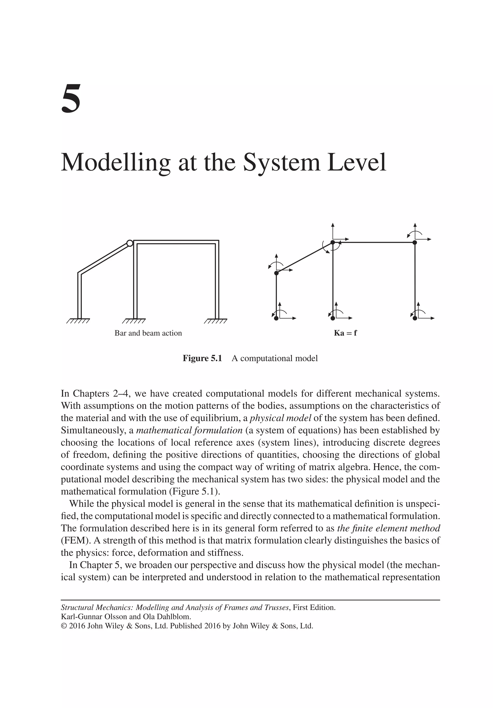
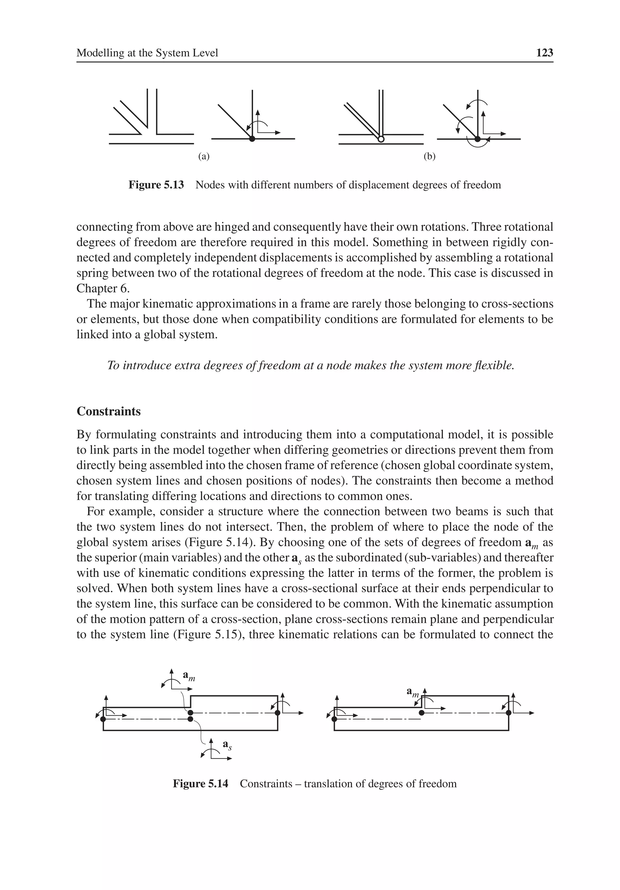
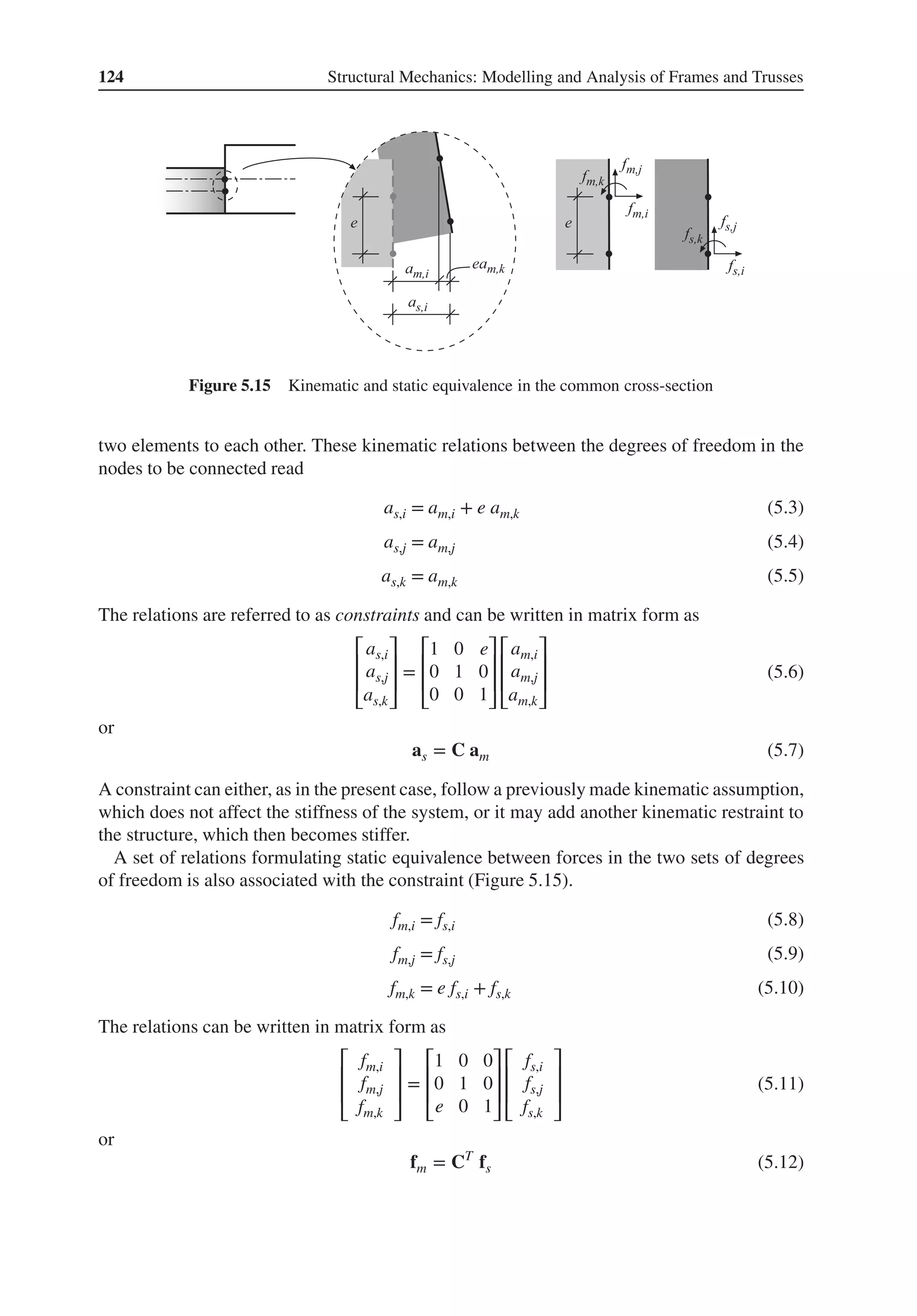
![Modelling at the System Level 125
Figure 5.16 Beam element before and after translation of degrees of freedom
The constraints can now be introduced into the element equation to relate the degrees of
freedom of the element to the degrees of freedom of a global system (Figure 5.16). If we
partition the system of equations of the element, we obtain
[
Ke
1
Ke
1s
(
Ke
1s
)T
Ke
s
]
[
ae
1
ae
s
]
=
[
fe
1
fe
s
]
(5.13)
where ae
s is the displacement degrees of freedom to be replaced by new degrees of freedom
ae
m. Substitution of the kinematic relation (5.7) into (5.13) gives
[
Ke
1
Ke
1s
C
(
Ke
1s
)T
Ke
sC
]
[
ae
1
ae
m
]
=
[
fe
1
fe
s
]
(5.14)
Left-multiplying the lower part of the system of equations by CT and using the force relation
(5.12) give [
Ke
1
Ke
1s
C
(
Ke
1s
C
)T
CTKe
sC
]
[
ae
1
ae
m
]
=
[
fe
1
fe
m
]
(5.15)
which is the system of equations of the element expressed in the new degrees of freedom. If we
solve the global system of equations, we can obtain the displacements ae
m. If we want to, we
can thereafter, with use of (5.7), determine the displacements for the original set of degrees of
freedom ae
s.
Alternatively, the constraints can be introduced directly at the system level (Figure 5.17).
The constraints (5.7) can then be formulated as
[
am
as
]
=
[
I
C
]
a; f =
[
I CT
]
[
fm
fs
]
(5.16)
Figure 5.17 Constraints introduced at the system level](https://image.slidesharecdn.com/structuralmechanicsmodellingandanalysisofframesandtrussespdfdrive-230720064114-5e1f9a93/75/Structural-mechanics-_-modelling-and-analysis-of-frames-and-trusses-PDFDrive-pdf-139-2048.jpg)
![126 Structural Mechanics: Modelling and Analysis of Frames and Trusses
where am with dimensions (m × 1) are the displacement degrees of freedom of the global sys-
tem, as with dimensions (s × 1) are auxiliary degrees of freedom and C is a transformation
matrix with dimensions (s × m). Partitioning the global system of equations gives
[
Kmm Kms
KT
ms Kss
]
[
am
as
]
=
[
fm
fs
]
(5.17)
Left-multiplication of the left and the right-hand sides in (5.17) with the matrix
[
I CT
]
gives
[
I CT
]
[
Kmm Kms
KT
ms Kss
]
[
am
as
]
=
[
I CT
]
[
fm
fs
]
(5.18)
Substituting (5.16) into (5.18), the following reduced system of equations is obtained
Ka = f (5.19)
where
K = Kmm +
(
KmsC
)T
+ KmsC + CT
KssC (5.20)
Figure 5.18 shows three examples of common situations where constraints are useful: In
panel (a), a structure with an inclined roller support is shown. In panel (b), the case stud-
ied earlier with translation of degrees of freedom along a rigid line is shown, and in panel (c),
a translation of degrees of freedom in connection to a rigid body displacement is shown.
If a constraint follows the kinematic approximations already done, the stiffness of
the system is maintained. If the constraint introduces a rigid connection between
two points, the stiffness increases.
(a) (b) (c)
Figure 5.18 Constraints – rotation of degrees of freedom, of a rigid line and of a rigid body](https://image.slidesharecdn.com/structuralmechanicsmodellingandanalysisofframesandtrussespdfdrive-230720064114-5e1f9a93/75/Structural-mechanics-_-modelling-and-analysis-of-frames-and-trusses-PDFDrive-pdf-140-2048.jpg)
![Modelling at the System Level 127
Example 5.1 Constraints – translation of degrees of freedom
Figure 1 Beam with discontinuous system line
Consider a beam ABC whose cross-section varies so that the system line of the beam is
discontinuous at B (Figure 1). An element relation for the beam part AB with degrees of
freedom that connect to the system line of the right beam part is to be determined. The left
beam part has the modulus of elasticity E, the cross-sectional area A, the moment of inertia
I and the length L. The distance between the system lines of the beam parts is e.
Computational model
Figure 2 Original beam element and beam element with translated degrees of freedom
We begin with a beam element with six degrees of freedom and with element relations
according to (4.86). The degrees of freedom to move are given index s (sub) and the degrees
of freedom to be established are given index m (main) (Figure 1).
Establishment of element relation
The system of equations (5.15) gives the sought element relation as
[
Ke
1
Ke
1s
C
(Ke
1s
C)T CT Ke
sC
]
[
ae
1
ae
m
]
=
[
fe
1
fe
m
]
(1)
We therefore need to determine the matrices Ke
1
, Ke
1s
, Ke
s and C. Partitioning of (4.86) with
respect to the degrees of freedom to move gives](https://image.slidesharecdn.com/structuralmechanicsmodellingandanalysisofframesandtrussespdfdrive-230720064114-5e1f9a93/75/Structural-mechanics-_-modelling-and-analysis-of-frames-and-trusses-PDFDrive-pdf-141-2048.jpg)
![128 Structural Mechanics: Modelling and Analysis of Frames and Trusses
⎡
⎢
⎢
⎢
⎢
⎢
⎢
⎢
⎢
⎢
⎢
⎣
DEA
L
0 0 −
DEA
L
0 0
0
12DEI
L3
6DEI
L2 0 −
12DEI
L3
6DEI
L2
0
6DEI
L2
4DEI
L
0 −
6DEI
L2
2DEI
L
−
DEA
L
0 0
DEA
L
0 0
0 −
12DEI
L3 −
6DEI
L2 0
12DEI
L3 −
6DEI
L2
0
6DEI
L2
2DEI
L
0 −
6DEI
L2
4DEI
L
⎤
⎥
⎥
⎥
⎥
⎥
⎥
⎥
⎥
⎥
⎥
⎦
⎡
⎢
⎢
⎢
⎢
⎢
⎢
⎢
⎢
⎢
⎢
⎣
u1
u2
u3
us,4
us,5
us,6
⎤
⎥
⎥
⎥
⎥
⎥
⎥
⎥
⎥
⎥
⎥
⎦
=
⎡
⎢
⎢
⎢
⎢
⎢
⎢
⎢
⎢
⎢
⎢
⎣
P1
P2
P3
Ps,4
Ps,5
Ps,6
⎤
⎥
⎥
⎥
⎥
⎥
⎥
⎥
⎥
⎥
⎥
⎦
(2)
or
[
Ke
1
Ke
1s
(Ke
1s
)T Ke
s
]
[
ae
1
ae
s
]
=
[
fe
1
fe
s
]
(3)
that is
Ke
1 =
⎡
⎢
⎢
⎢
⎢
⎣
DEA
L
0 0
0
12DEI
L3
6DEI
L2
0
6DEI
L2
4DEI
L
⎤
⎥
⎥
⎥
⎥
⎦
(4)
Ke
1s =
⎡
⎢
⎢
⎢
⎢
⎣
−
DEA
L
0 0
0 −
12DEI
L3
6DEI
L2
0 −
6DEI
L2
2DEI
L
⎤
⎥
⎥
⎥
⎥
⎦
(5)
Ke
s =
⎡
⎢
⎢
⎢
⎢
⎣
DEA
L
0 0
0
12DEI
L3 −
6DEI
L2
0 −
6DEI
L2
4DEI
L
⎤
⎥
⎥
⎥
⎥
⎦
(6)
The matrix C is determined by constraints and/or static equivalence. When the beam
deforms we have the kinematic condition that plane cross-sections remain plane; see
Figure 3a. At the interface B, these conditions can be reformulated as the constraints](https://image.slidesharecdn.com/structuralmechanicsmodellingandanalysisofframesandtrussespdfdrive-230720064114-5e1f9a93/75/Structural-mechanics-_-modelling-and-analysis-of-frames-and-trusses-PDFDrive-pdf-142-2048.jpg)
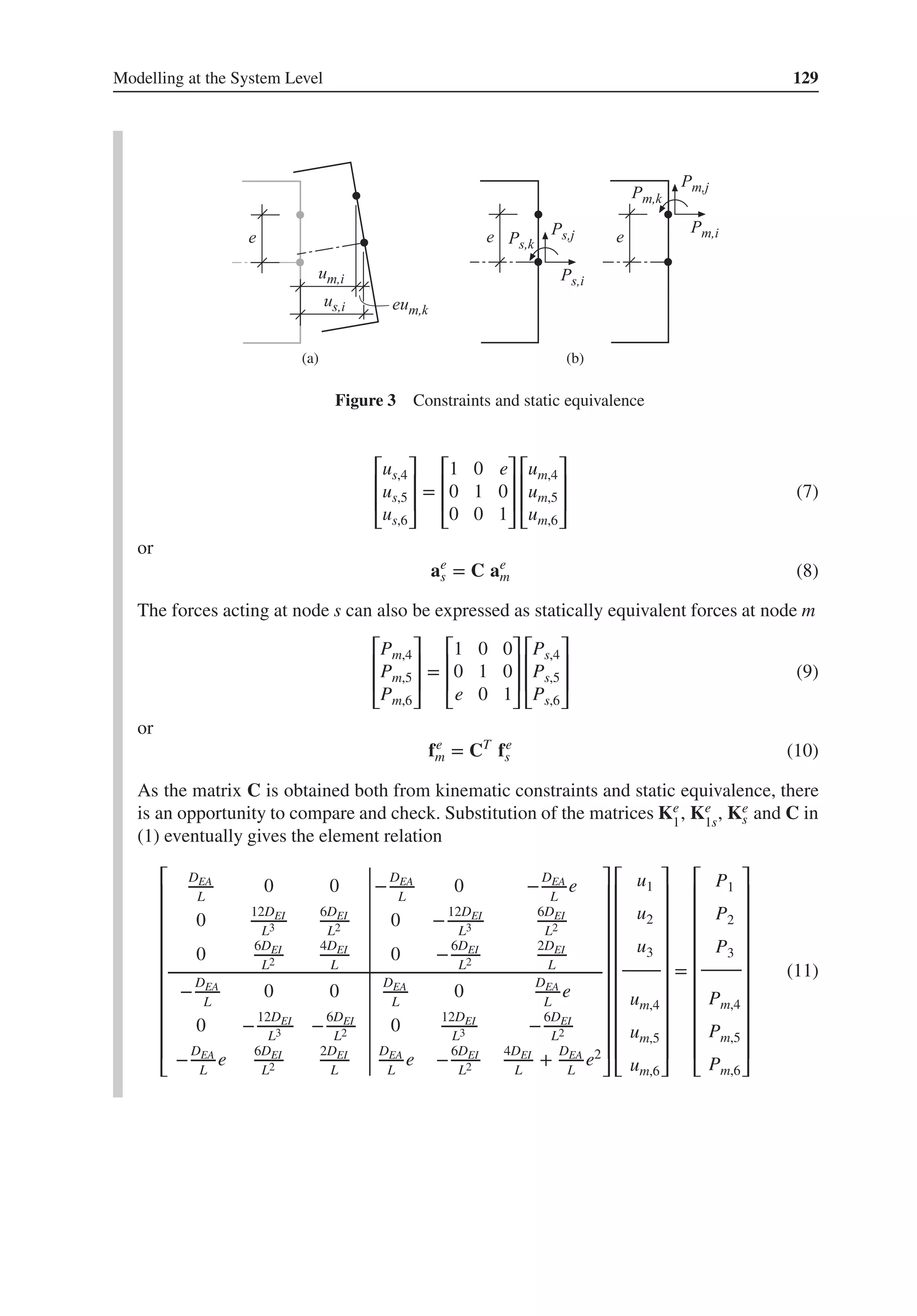
![130 Structural Mechanics: Modelling and Analysis of Frames and Trusses
Prescribed Displacements
When we prescribe the displacement of a degree of freedom – either to zero or to a non-zero
value – the degree of freedom will be prevented from further displacements. An external load-
ing acting on the structure will perceive the structure as infinitely stiff in the direction of the
prescribed degree of freedom. We have previously, in Equation (1.40), observed that by using
partition we do not have to use the equations that correspond to prescribed degrees of freedom
to solve the system of equations
[
A1 A2
A3
̃
K
]
[
g
̃
a
]
=
[
r
̃
f
]
(5.21)
If the displacements g are prescribed to zero, g = 𝟎, (5.21) can be divided into two parts and
written as
̃
K ̃
a = ̃
f (5.22)
r = A2 ̃
a (5.23)
that is we get the reduced stiffness matrix ̃
K directly by deleting the rows and columns in
K associated with the prescribed displacements g. The support forces r can be determined
by multiplication when the unknown displacements ̃
a have been determined. For prescribed
non-zero displacements, g ≠ 𝟎, we, instead of (5.22) and (5.23), get
̃
K ̃
a = ̃
f − A3 g (5.24)
r = A1 g + A2 ̃
a (5.25)
where A3 g corresponds to the values of the support forces necessary to keep the displacements
at the prescribed values.
When a displacement is prescribed, a global restraint is introduced, which
increases the stiffness of the system.
5.2.2 The Forces and Equilibria of the System
The degrees of freedom of a system are references for the displacements of the structure,
but also references for the internal equilibria of the structure. For each degree of freedom
an internal equilibrium equation can be established (Figure 5.19) and for each node in a plane
frame at least three equilibrium equations can then be established. Rigidly connected elements
contribute with forces to the same equilibria, while bodies with independent displacements
contribute to different equilibrium conditions. The latter implies that two bodies can meet at a
point without transmitting forces between each other.
Figure 5.20 shows a node where two elements are hinged to an otherwise rigidly con-
nected node (see also Figure 5.13). This means that to this node five equilibrium equations
are associated
fi = P(𝛼)
4
+ P(𝛽)
4
+ P(𝛾)
1
+ P(𝛿)
1
(5.26)
fj = P(𝛼)
5
+ P(𝛽)
5
+ P(𝛾)
2
+ P(𝛿)
2
(5.27)](https://image.slidesharecdn.com/structuralmechanicsmodellingandanalysisofframesandtrussespdfdrive-230720064114-5e1f9a93/75/Structural-mechanics-_-modelling-and-analysis-of-frames-and-trusses-PDFDrive-pdf-144-2048.jpg)
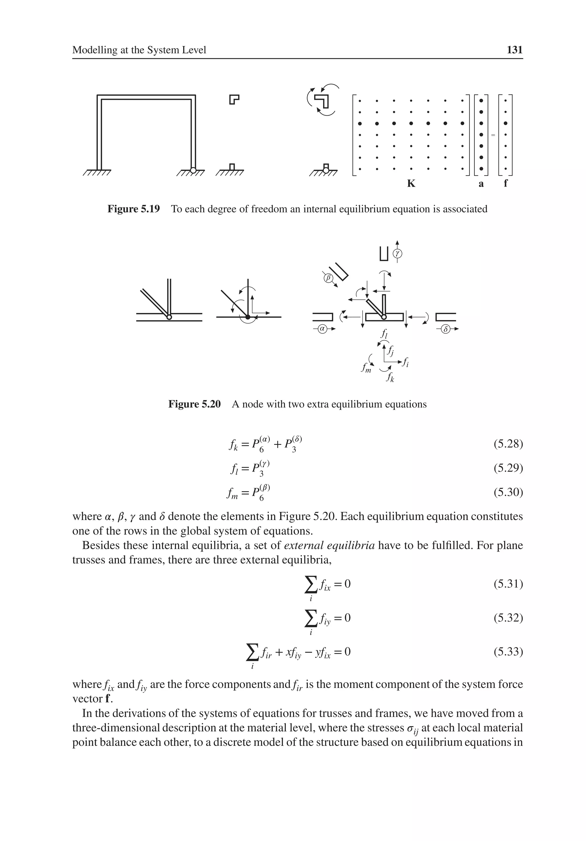
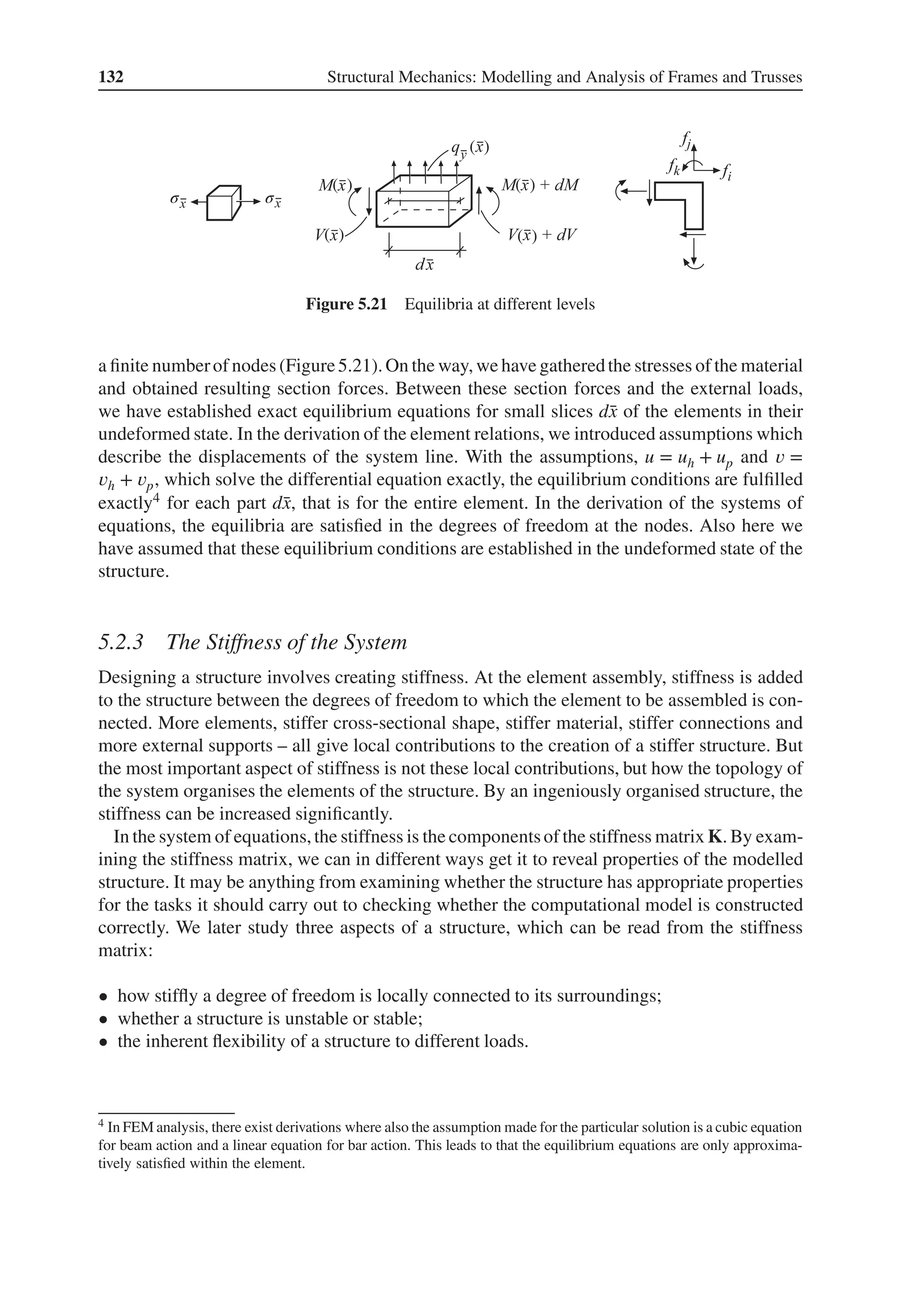
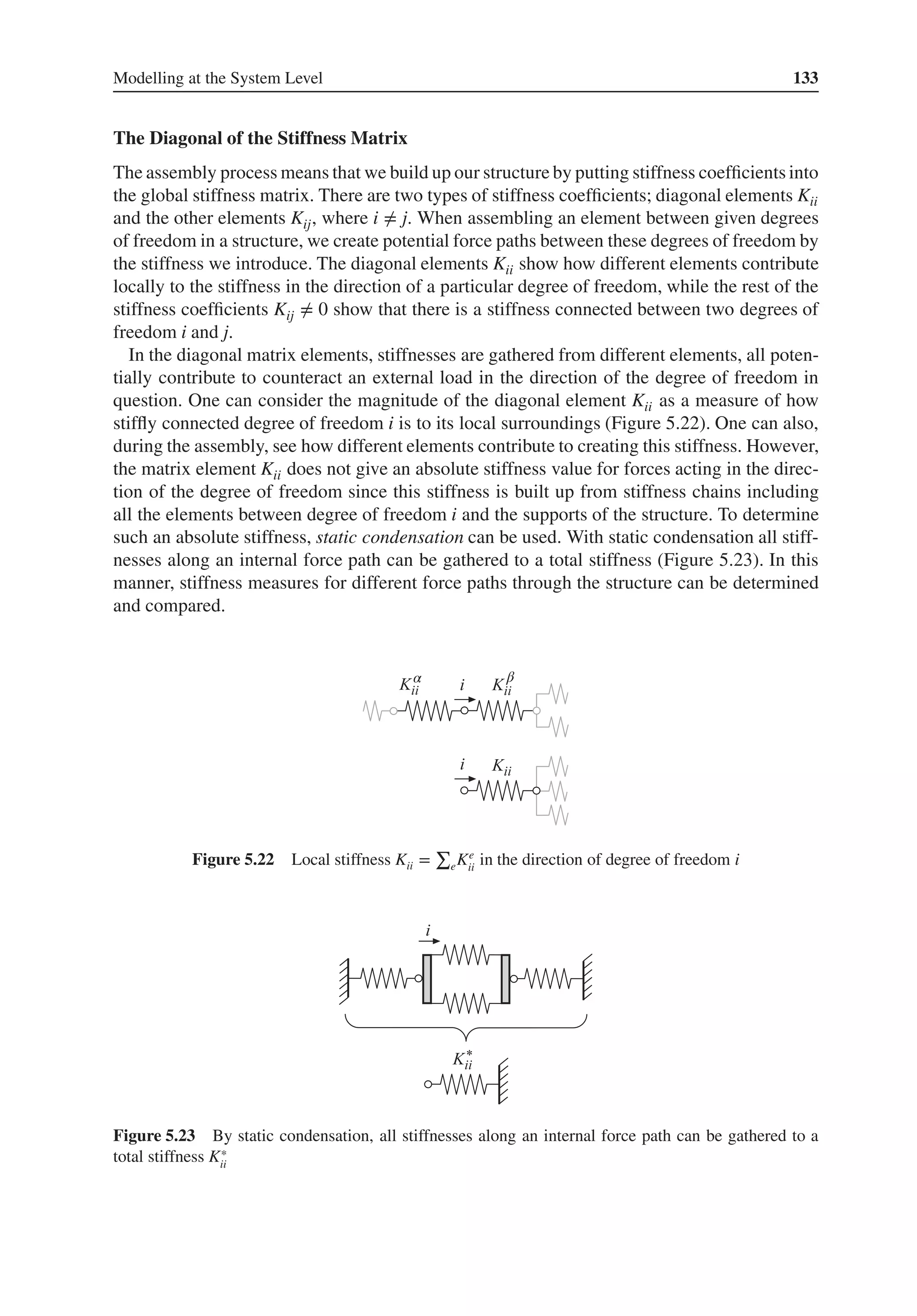
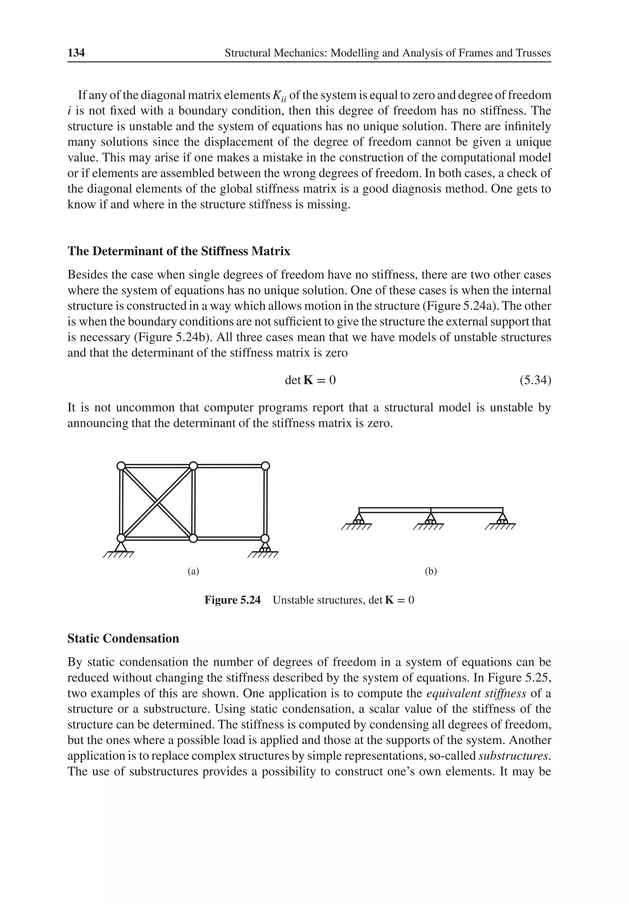
![Modelling at the System Level 135
Figure 5.25 Examples of applications for static condensation
elements that replace a repeated part of a structure. Such an element is first built as a separate
structure. After that, the internal degrees of freedom are condensed out, so that the remaining
structure only has a few degrees of freedom on the external edge.
In Section 1.7, we have described how a system of equations can be partitioned. The purpose
there was to handle prescribed variables, that is boundary conditions, when solving the system
of equations. To perform a static condensation, we partition the system of equations in the
same manner, that is the system of equations
Ka = f (5.35)
is written as [
Kaa Kab
Kba Kbb
]
[
aa
̃
a
]
=
[
fa
fb
]
(5.36)
or
Kaaaa + Kab ̃
a = fa (5.37)
Kbaaa + Kbb ̃
a = fb (5.38)
We have divided the displacement vector a into two parts aa and ̃
a and we want to eliminate
aa without changing the properties of the computational model. We rewrite (5.37) as
aa = K−1
aa (fa − Kab ̃
a) (5.39)
and substitute this relation into (5.38), which gives
KbaK−1
aa (fa − Kab ̃
a) + Kbb ̃
a = fb (5.40)
or
̃
K̃
a = ̃
f (5.41)](https://image.slidesharecdn.com/structuralmechanicsmodellingandanalysisofframesandtrussespdfdrive-230720064114-5e1f9a93/75/Structural-mechanics-_-modelling-and-analysis-of-frames-and-trusses-PDFDrive-pdf-149-2048.jpg)
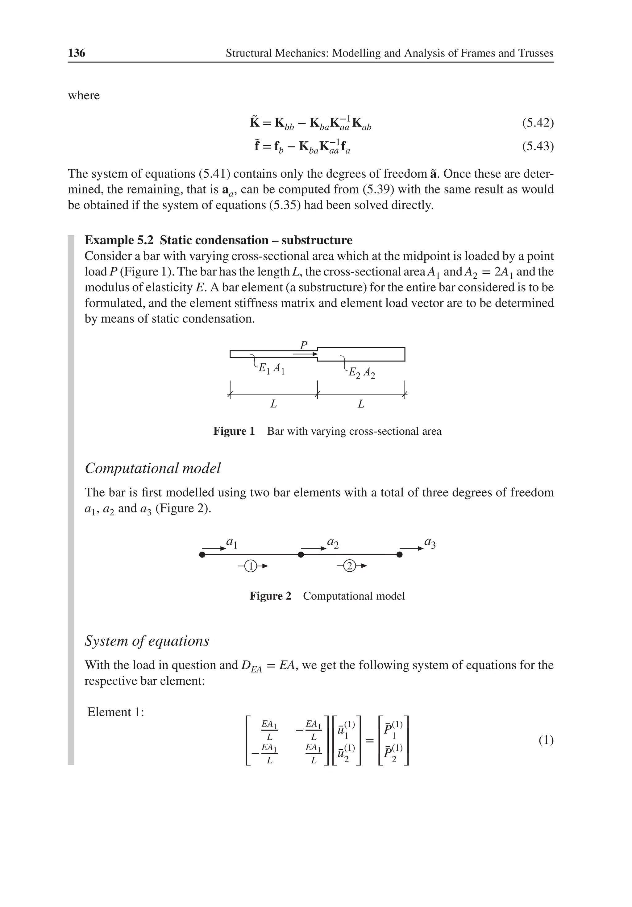
![Modelling at the System Level 137
Element 2:
⎡
⎢
⎢
⎣
2EA1
L
−
2EA1
L
−
2EA1
L
2EA1
L
⎤
⎥
⎥
⎦
⎡
⎢
⎢
⎣
̄
u(2)
1
̄
u(2)
2
⎤
⎥
⎥
⎦
=
⎡
⎢
⎢
⎣
̄
P(2)
1
̄
P(2)
2
⎤
⎥
⎥
⎦
(2)
Assembling and introducing the point load P gives the system of equations
⎡
⎢
⎢
⎢
⎢
⎣
EA1
L
−
EA1
L
0
−
EA1
L
3EA1
L
−
2EA1
L
0 −
2EA1
L
2EA1
L
⎤
⎥
⎥
⎥
⎥
⎦
⎡
⎢
⎢
⎢
⎢
⎣
a1
a2
a3
⎤
⎥
⎥
⎥
⎥
⎦
=
⎡
⎢
⎢
⎢
⎢
⎣
f1
P
f3
⎤
⎥
⎥
⎥
⎥
⎦
(3)
Static condensation
A static condensation is based on equation (5.36)
[
Kaa Kab
Kba Kbb
]
[
aa
̃
a
]
=
[
fa
fb
]
(4)
where the rows belonging to the degrees of freedom to be condensed are placed first. This
can in many cases be achieved already at the initial numbering of the degrees of freedom
if one considers giving the degrees of freedom that will condense out the lowest number. If
this has not been done a reordering has to be done. The systematics for such a reordering is
based on change of the sequence of equations, while the sequence of terms in the equations
is changed accordingly. Reordering of (3) and partitioning gives
⎡
⎢
⎢
⎢
⎢
⎣
3EA1
L
−
EA1
L
−
2EA1
L
−
EA1
L
EA1
L
0
−
2EA1
L
0
2EA1
L
⎤
⎥
⎥
⎥
⎥
⎦
⎡
⎢
⎢
⎢
⎢
⎣
a2
a1
a3
⎤
⎥
⎥
⎥
⎥
⎦
=
⎡
⎢
⎢
⎢
⎢
⎣
P
f1
f3
⎤
⎥
⎥
⎥
⎥
⎦
(5)
The stiffness matrix for the new bar element is obtained from (5.42)
̃
K = Kbb − KbaK−1
aa Kab (6)
and a force vector, which takes into account the point load acting in the middle of the bar
is obtained from (5.43)
̃
f = fb − KbaK−1
aa fa (7)
Substituting the components from (5) into (6) and (7), one obtains
̃
K =
⎡
⎢
⎢
⎣
EA1
L
0
0
2EA1
L
⎤
⎥
⎥
⎦
−
⎡
⎢
⎢
⎣
−
EA1
L
−
2EA1
L
⎤
⎥
⎥
⎦
[
3EA1
L
]−1 [
−
EA1
L
−
2EA1
L
]
=
[EA1
L
0
0
2EA1
L
]
−
⎡
⎢
⎢
⎣
EA1
3L
2EA1
3L
2EA1
3L
4EA1
3L
⎤
⎥
⎥
⎦
=
⎡
⎢
⎢
⎣
2EA1
3L
−
2EA1
3L
−
2EA1
3L
2EA1
3L
⎤
⎥
⎥
⎦
(8)](https://image.slidesharecdn.com/structuralmechanicsmodellingandanalysisofframesandtrussespdfdrive-230720064114-5e1f9a93/75/Structural-mechanics-_-modelling-and-analysis-of-frames-and-trusses-PDFDrive-pdf-151-2048.jpg)
![138 Structural Mechanics: Modelling and Analysis of Frames and Trusses
̃
f =
[
f1
f3
]
−
⎡
⎢
⎢
⎣
−
EA1
L
−
2EA1
L
⎤
⎥
⎥
⎦
[
3EA1
L
]−1 [
P
]
=
[
f1
f3
]
+
⎡
⎢
⎢
⎣
P
3
2P
3
⎤
⎥
⎥
⎦
(9)
Note that the components of the element load vector are different. A stiffer element part
carries a larger share of the load. We have earlier in Examples 3.1 and 4.1 computed the
equivalent element load vectors, and then the uniformly distributed load was placed at the
two nodes with equal shares. This has then been based on the assumption of a constant
axial stiffness DEA and a constant bending stiffness DEI.
Example 5.3 Static condensation – equivalent spring stiffness
Consider a console beam that in its free end is loaded by a point load P (Figure 1). The
beam has length L, the moment of inertia I and the modulus of elasticity E. To the right of
the console beam an elastic spring is shown which represents the vertical stiffness of the
beam at the force application point. The value of the spring stiffness k is to be determined
by static condensation.
Figure 1 Console beam with point load
Computational model
Figure 2 Computational model
The console beam is modelled using a beam element with four degrees of freedom
̄
u1 – ̄
u4 (Figure 2). We choose to consider the support conditions of the computational
model in connection to the static condensation. With this strategy, quite complex two- and
three-dimensional support structures may be reduced to a static equivalent spring with the
displacement prescribed at one node; see Figures 5.23 and 5.25.](https://image.slidesharecdn.com/structuralmechanicsmodellingandanalysisofframesandtrussespdfdrive-230720064114-5e1f9a93/75/Structural-mechanics-_-modelling-and-analysis-of-frames-and-trusses-PDFDrive-pdf-152-2048.jpg)
![Modelling at the System Level 139
Systems of equations and static condensation
From (4.80), we have the system of equations for a beam element with four degrees of
freedom. With DEI = EI, we get
EI
L3
⎡
⎢
⎢
⎢
⎣
12 6L −12 6L
6L 4L2 −6L 2L2
−12 −6L 12 −6L
6L 2L2 −6L 4L2
⎤
⎥
⎥
⎥
⎦
⎡
⎢
⎢
⎢
⎣
̄
u1
̄
u2
̄
u3
̄
u4
⎤
⎥
⎥
⎥
⎦
=
⎡
⎢
⎢
⎢
⎣
̄
P1
̄
P2
̄
P3
̄
P4
⎤
⎥
⎥
⎥
⎦
(1)
For the console beam, the translation a1 and the rotation a2 are prescribed to be zero.
According to (5.22), the system of equations (1) may thus directly be reduced to
EI
L3
[
12 −6L
−6L 4L2
]
[
̄
u3
̄
u4
]
=
[
̄
P3
̄
P4
]
(2)
Relocation of the lines of the system of equations and partitioning according to (5.36) gives
EI
L3
[
4L2 −6L
−6L 12
]
[
̄
u4
̄
u3
]
=
[
̄
P4
̄
P3
]
(3)
Equation (5.42) finally gives the spring stiffness as
̃
K =
[
12EI
L3
]
−
[
−6EI
L2
][
4EI
L
]−1 [
−6EI
L2
]
=
[
12EI
L3
]
−
[
9EI
L3
]
=
[
3EI
L3
]
(4)
that is we have the static equivalent spring stiffness k = 3EI
L3 .
Example 5.4 Reduction of a degree of freedom for an elementary case
Figure 1 A beam element with four degrees of freedom and a beam element where degree of
freedom ̄
u4 has been condensed out.
Consider a beam element with four degrees of freedom with a uniformly distributed load.
We need to eliminate the rotation ̄
u4 to obtain a beam element with three degrees of freedom
according to Figure 1. For this element a reduced element stiffness matrix (3 × 3) and a](https://image.slidesharecdn.com/structuralmechanicsmodellingandanalysisofframesandtrussespdfdrive-230720064114-5e1f9a93/75/Structural-mechanics-_-modelling-and-analysis-of-frames-and-trusses-PDFDrive-pdf-153-2048.jpg)
![140 Structural Mechanics: Modelling and Analysis of Frames and Trusses
reduced nodal load vector (3 × 1) for a uniformly distributed load shall be determined.
From (4.81), we have the element relation
DEI
L3
⎡
⎢
⎢
⎢
⎢
⎢
⎢
⎣
12 6L −12 6L
6L 4L2 −6L 2L2
−12 −6L 12 −6L
6L 2L2 −6L 4L2
⎤
⎥
⎥
⎥
⎥
⎥
⎥
⎦
⎡
⎢
⎢
⎢
⎢
⎢
⎢
⎣
̄
u1
̄
u2
̄
u3
̄
u4
⎤
⎥
⎥
⎥
⎥
⎥
⎥
⎦
=
⎡
⎢
⎢
⎢
⎢
⎢
⎢
⎣
̄
P1
̄
P2
̄
P3
̄
P4
⎤
⎥
⎥
⎥
⎥
⎥
⎥
⎦
+ q̄
y
⎡
⎢
⎢
⎢
⎢
⎢
⎢
⎣
L
2
L2
12
L
2
−L2
12
⎤
⎥
⎥
⎥
⎥
⎥
⎥
⎦
(1)
where the components of ̄
fe
l
represent a uniformly distributed load according to Example
4.1. Using Equation (4), the displacement ̄
u4 can be written as
̄
u4 =
L
4DEI
(
̄
P4 −
q̄
yL2
12
)
−
[
3
2L
1
2
− 3
2L
] ⎡
⎢
⎢
⎣
̄
u1
̄
u2
̄
u3
⎤
⎥
⎥
⎦
(2)
Substituting this into the other three equations then gives
DEI
L3
⎡
⎢
⎢
⎢
⎢
⎣
3 3L −3
3L 3L2 −3L
−3 −3L 3
⎤
⎥
⎥
⎥
⎥
⎦
⎡
⎢
⎢
⎢
⎢
⎣
̄
u1
̄
u2
̄
u3
⎤
⎥
⎥
⎥
⎥
⎦
=
⎡
⎢
⎢
⎢
⎢
⎣
̄
P1
̄
P2
̄
P3
⎤
⎥
⎥
⎥
⎥
⎦
+ ̄
P4
⎡
⎢
⎢
⎢
⎢
⎣
− 3
2L
−1
2
3
2L
⎤
⎥
⎥
⎥
⎥
⎦
+ q̄
y
⎡
⎢
⎢
⎢
⎢
⎣
5L
8
L2
8
3L
8
⎤
⎥
⎥
⎥
⎥
⎦
(3)
We have here performed the static condensation without using the systematics of
(5.36)–(5.43). Equation (3) is an element relation for a beam element with three degrees
of freedom. The element can still rotate around the node to the right where the rotational
degree of freedom has been condensed out, but the rotation here cannot be related to
rotations of other connected elements.
Canonical Stiffness
From the stiffness matrix K of a structure, a set of scalar stiffnesses referred to as canonical
stiffnesses can be computed. Such a computation begins from the assumption that there is a set
of displacement modes (deformation patterns) a that are proportional to a corresponding set of
load cases f acting on the structure (Figure 5.26). For structures modelled with only translation
degrees of freedom, such as trusses, this can be described as
f = 𝜆a (5.44)
Thus, the eigenvalues 𝜆i get the dimension [force/length], that is the same dimension as the
stiffness of a spring. The system of equations for the structure can now be written as
Ka = f = 𝜆a (5.45)
or
(K − 𝜆I)a = 𝟎 (5.46)](https://image.slidesharecdn.com/structuralmechanicsmodellingandanalysisofframesandtrussespdfdrive-230720064114-5e1f9a93/75/Structural-mechanics-_-modelling-and-analysis-of-frames-and-trusses-PDFDrive-pdf-154-2048.jpg)
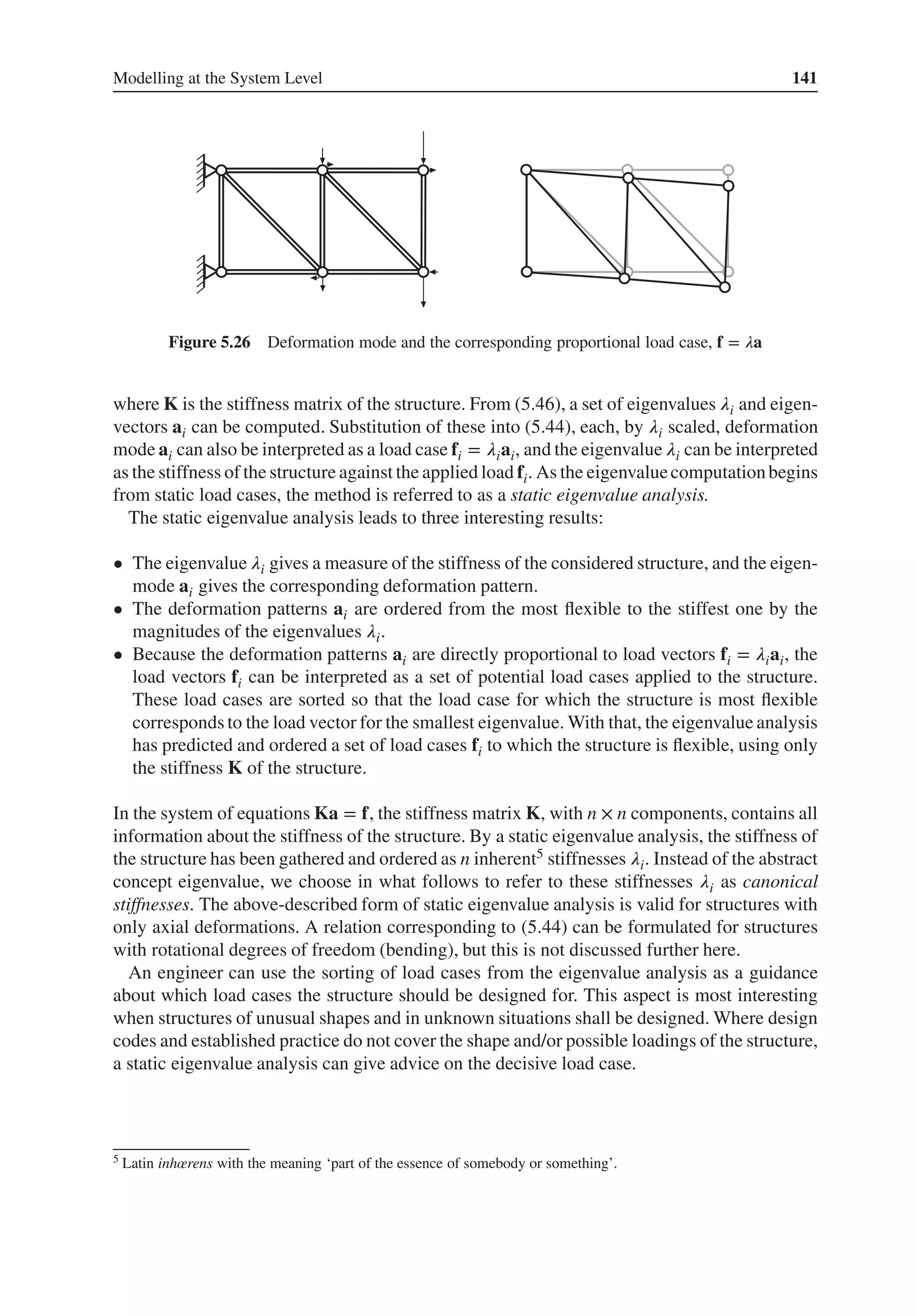
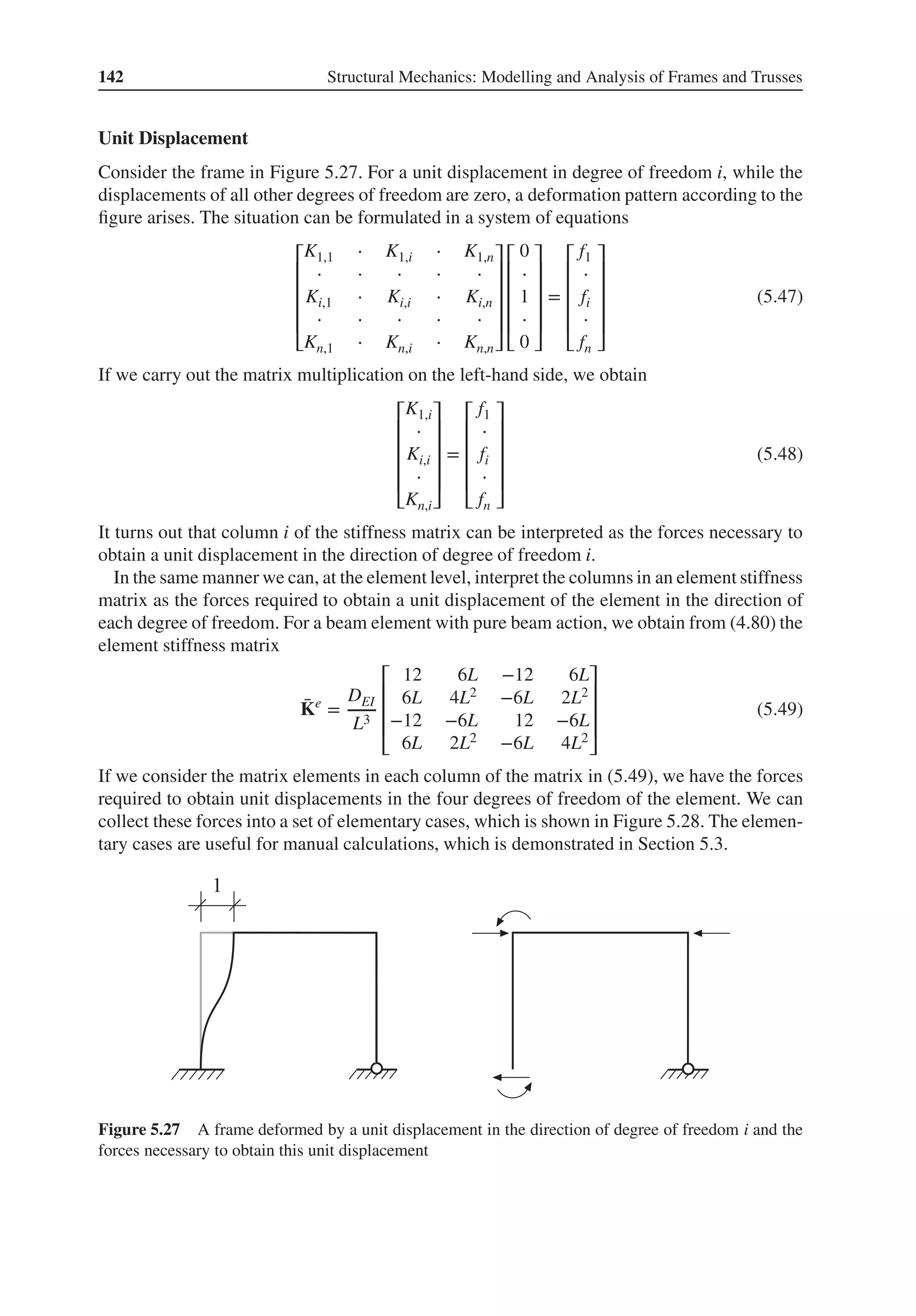
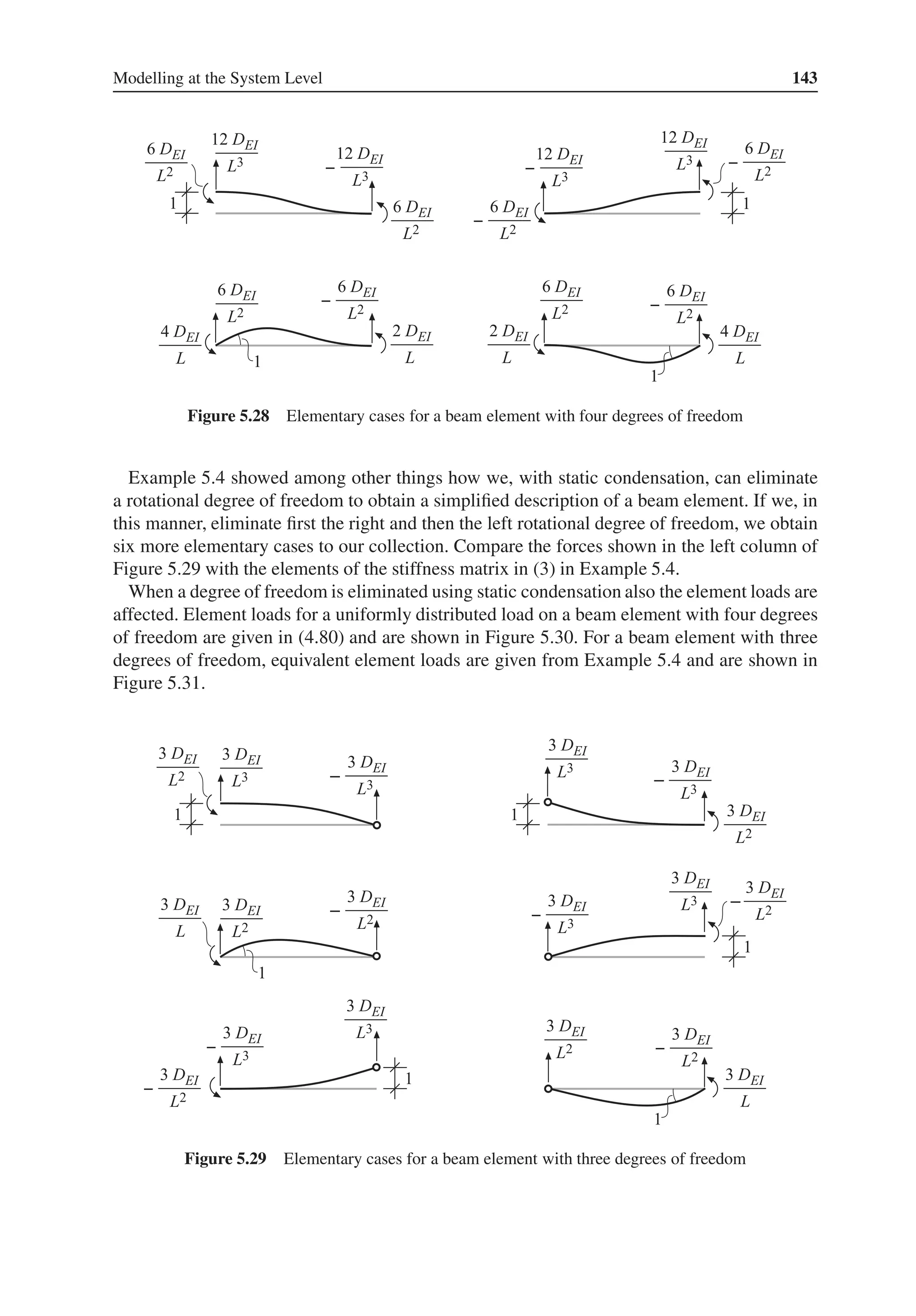
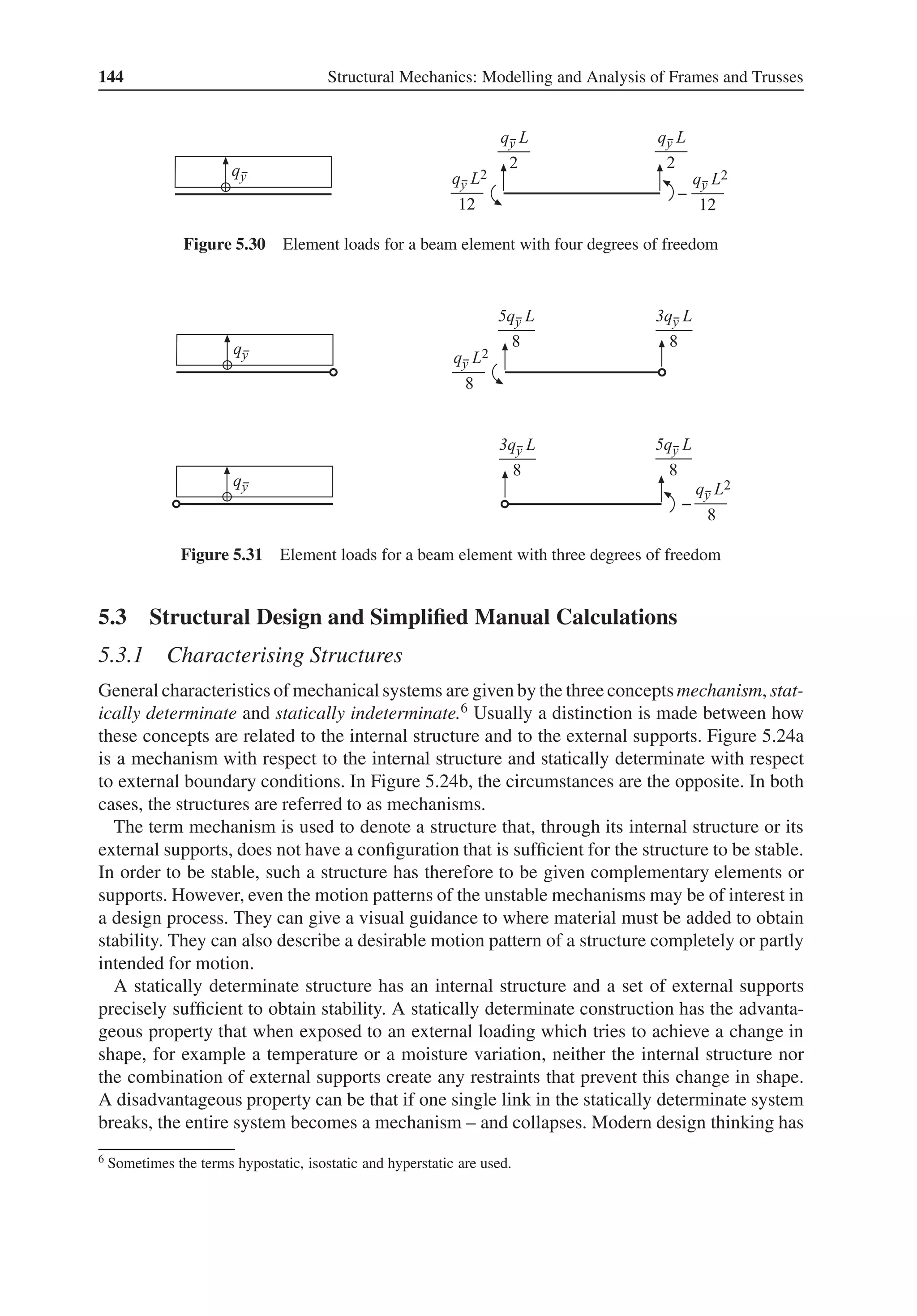
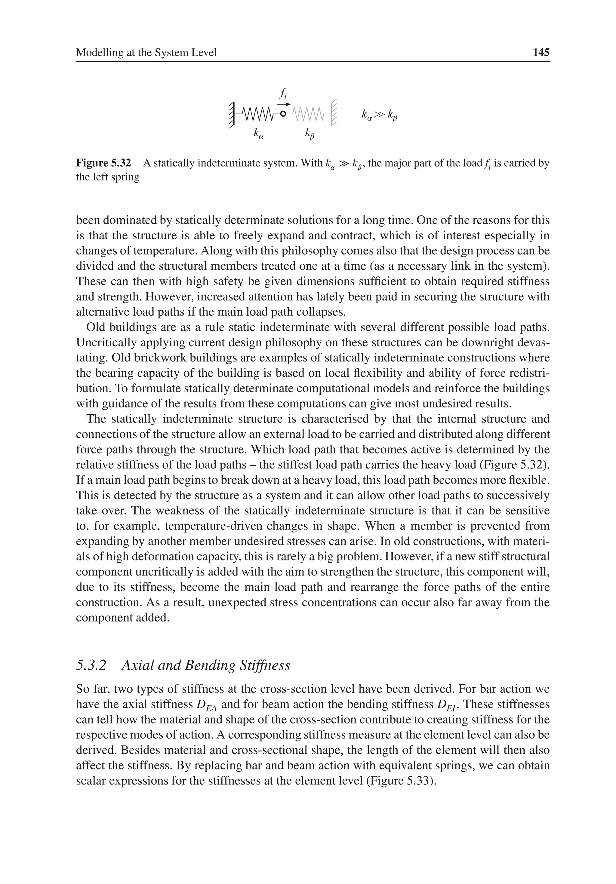
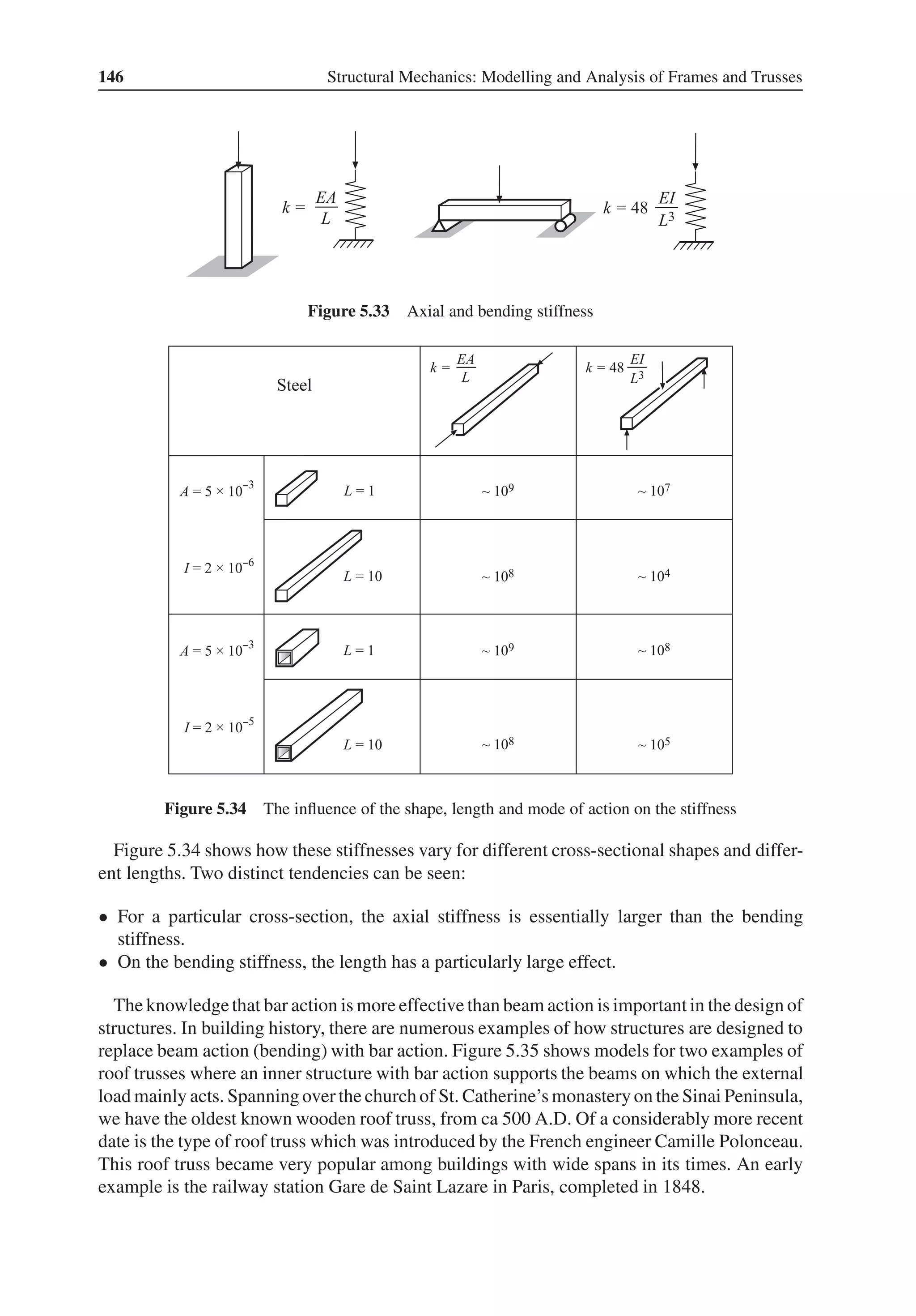
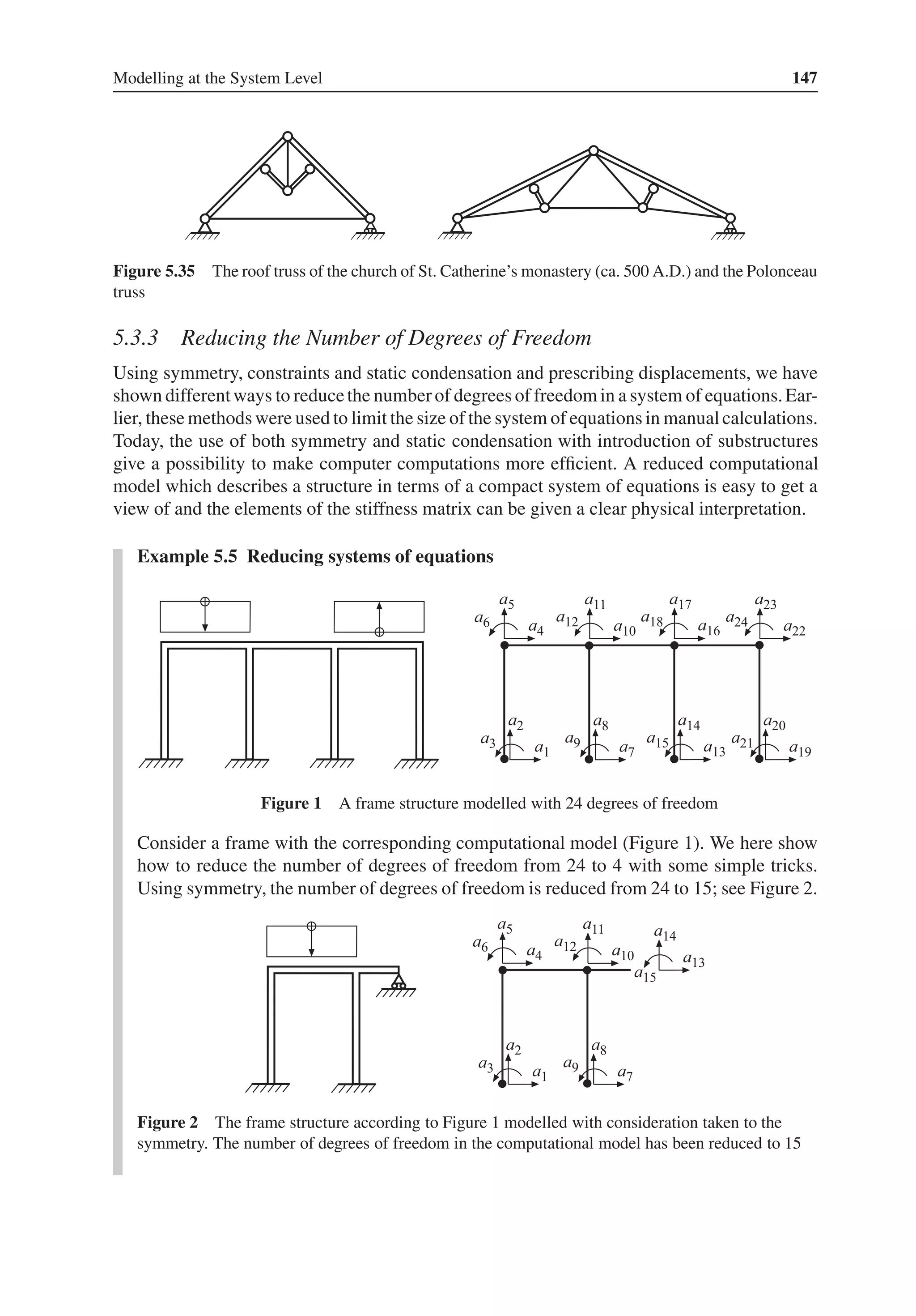
![148 Structural Mechanics: Modelling and Analysis of Frames and Trusses
The next reduction is possible because the mode of action of the frame in question is
dominated by beam action. In the previous section, we pointed out differences in stiffness
between structures carrying load by bar action and structures carrying load mainly by beam
action. For the present frame, beam action will dominate the magnitudes of deformations
and internal stresses. With beam action as the dominating mode of action, the axial defor-
mations can be neglected. This can be formulated as constraints where a5, a10, a11 and a13
can be regarded as sub-variables and the other displacements as main variables. Then we
obtain the constraints
a5 = a2; a10 = a4; a11 = a8; a13 = a4 (1)
which can be formulated in matrix form as
[
am
as
]
=
[
I
C
]
a (2)
If the degrees of freedom are written in numerical order and consequently with main and
sub-variables mixed, (2) becomes
⎡
⎢
⎢
⎢
⎢
⎢
⎢
⎢
⎢
⎢
⎢
⎢
⎢
⎢
⎢
⎢
⎢
⎢
⎢
⎣
a1
a2
a3
a4
a5
a6
a7
a8
a9
a10
a11
a12
a13
a14
a15
⎤
⎥
⎥
⎥
⎥
⎥
⎥
⎥
⎥
⎥
⎥
⎥
⎥
⎥
⎥
⎥
⎥
⎥
⎥
⎦
=
⎡
⎢
⎢
⎢
⎢
⎢
⎢
⎢
⎢
⎢
⎢
⎢
⎢
⎢
⎢
⎢
⎢
⎢
⎢
⎣
1 0 0 0 0 0 0 0 0 0 0
0 1 0 0 0 0 0 0 0 0 0
0 0 1 0 0 0 0 0 0 0 0
0 0 0 1 0 0 0 0 0 0 0
0 1 0 0 0 0 0 0 0 0 0
0 0 0 0 1 0 0 0 0 0 0
0 0 0 0 0 1 0 0 0 0 0
0 0 0 0 0 0 1 0 0 0 0
0 0 0 0 0 0 0 1 0 0 0
0 0 0 1 0 0 0 0 0 0 0
0 0 0 0 0 0 1 0 0 0 0
0 0 0 0 0 0 0 0 1 0 0
0 0 0 1 0 0 0 0 0 0 0
0 0 0 0 0 0 0 0 0 1 0
0 0 0 0 0 0 0 0 0 0 1
⎤
⎥
⎥
⎥
⎥
⎥
⎥
⎥
⎥
⎥
⎥
⎥
⎥
⎥
⎥
⎥
⎥
⎥
⎥
⎦
⎡
⎢
⎢
⎢
⎢
⎢
⎢
⎢
⎢
⎢
⎢
⎢
⎢
⎣
a1
a2
a3
a4
a5
a6
a7
a8
a9
a10
a11
⎤
⎥
⎥
⎥
⎥
⎥
⎥
⎥
⎥
⎥
⎥
⎥
⎥
⎦
(3)
where the old numbering of the degrees of freedom is shown in Figure 2 and the new
numbering of the degrees of freedom is shown in Figure 3a. Note that ai on the left hand
side of (3) does not denote the same thing as ai on the right-hand side.
(a) (b)
Figure 3 A computational model with neglected axial deformations (a) and the substituted
boundary conditions (b).](https://image.slidesharecdn.com/structuralmechanicsmodellingandanalysisofframesandtrussespdfdrive-230720064114-5e1f9a93/75/Structural-mechanics-_-modelling-and-analysis-of-frames-and-trusses-PDFDrive-pdf-162-2048.jpg)
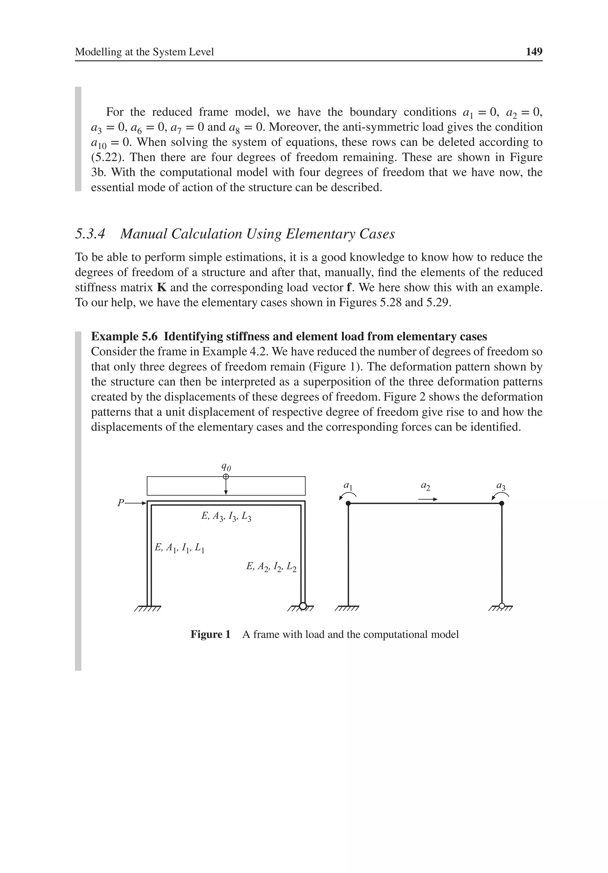
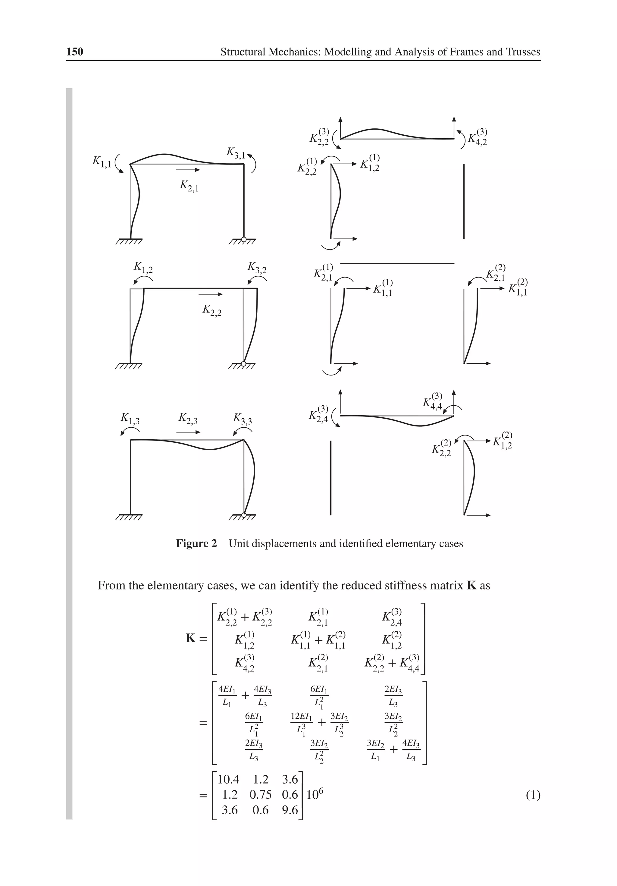
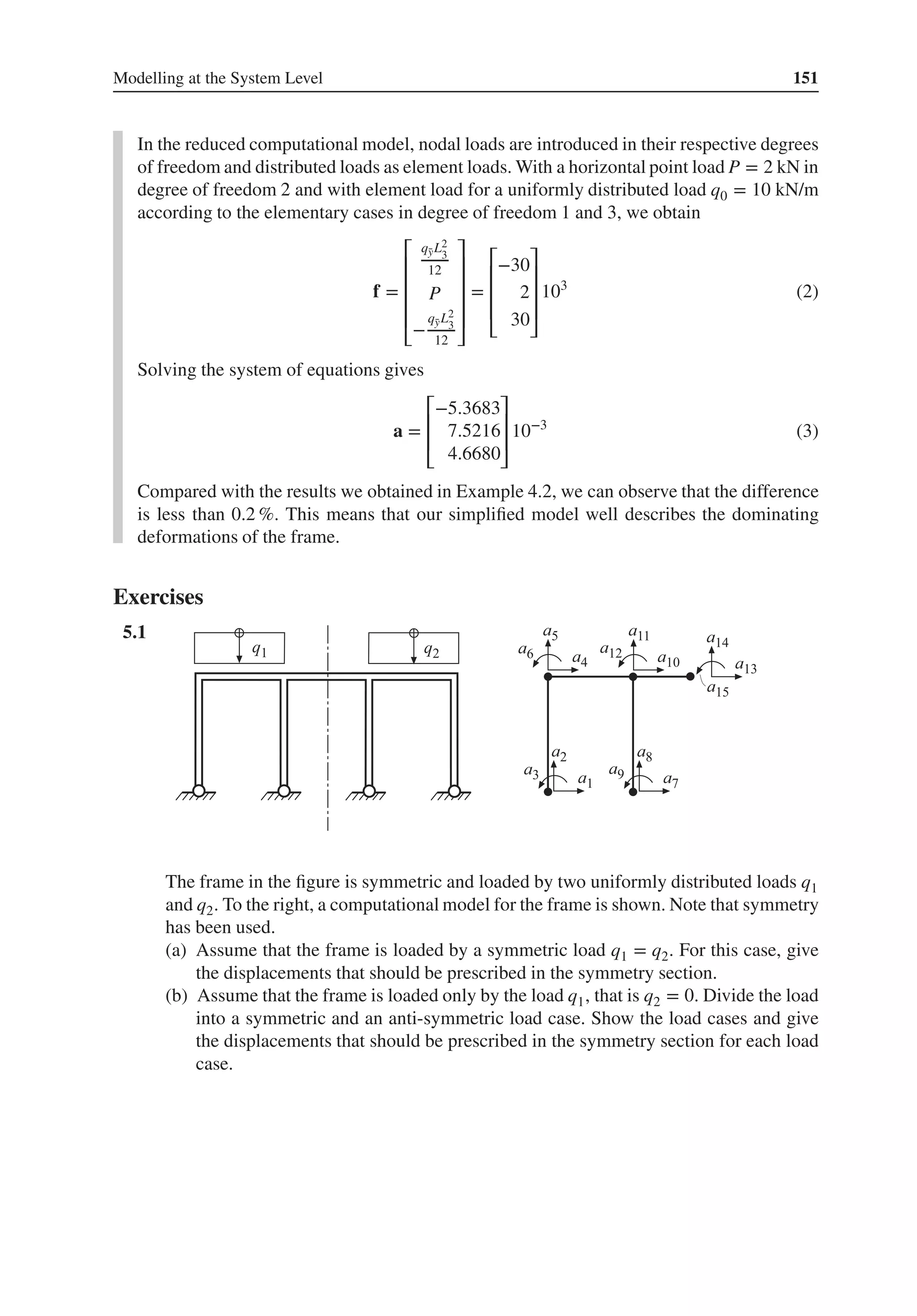
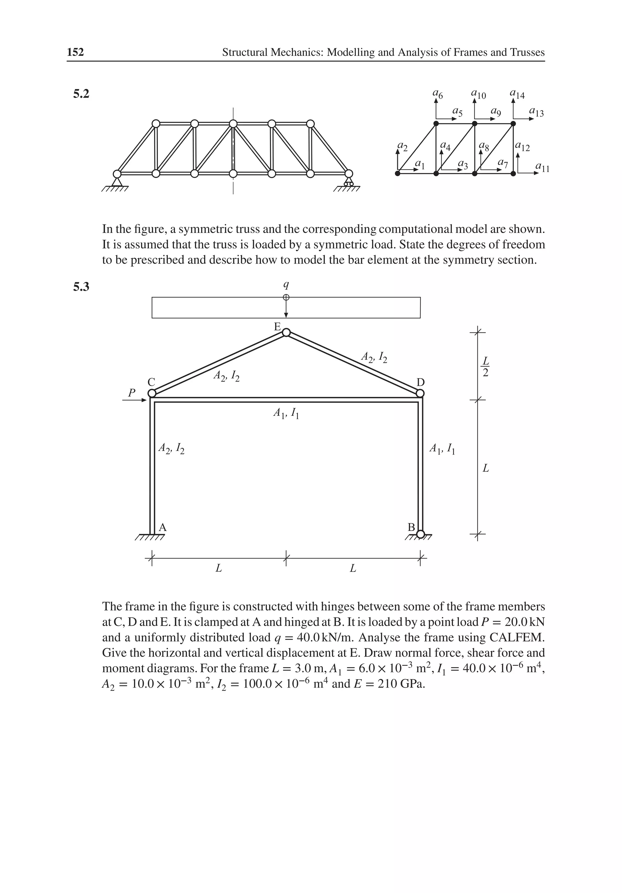
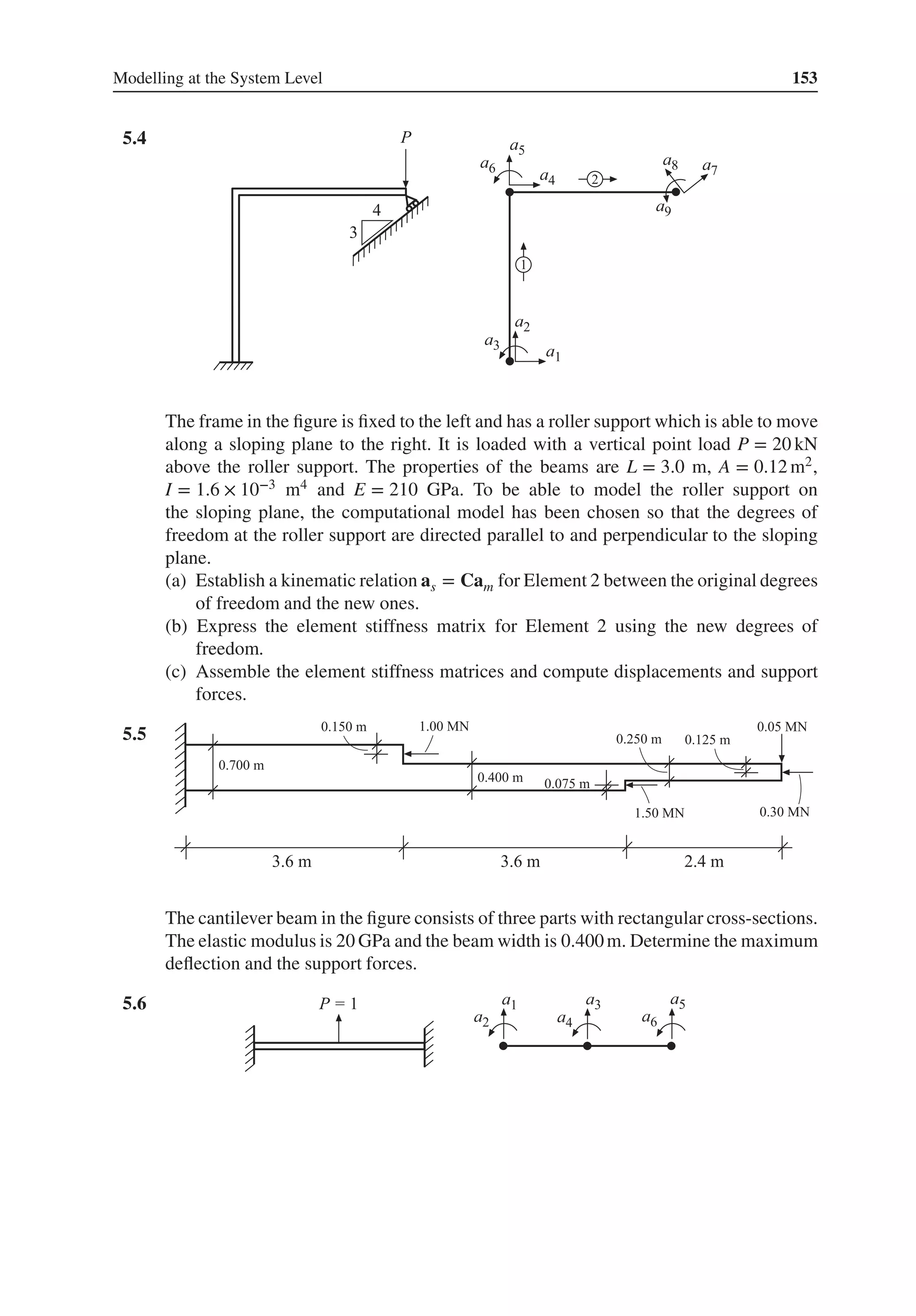
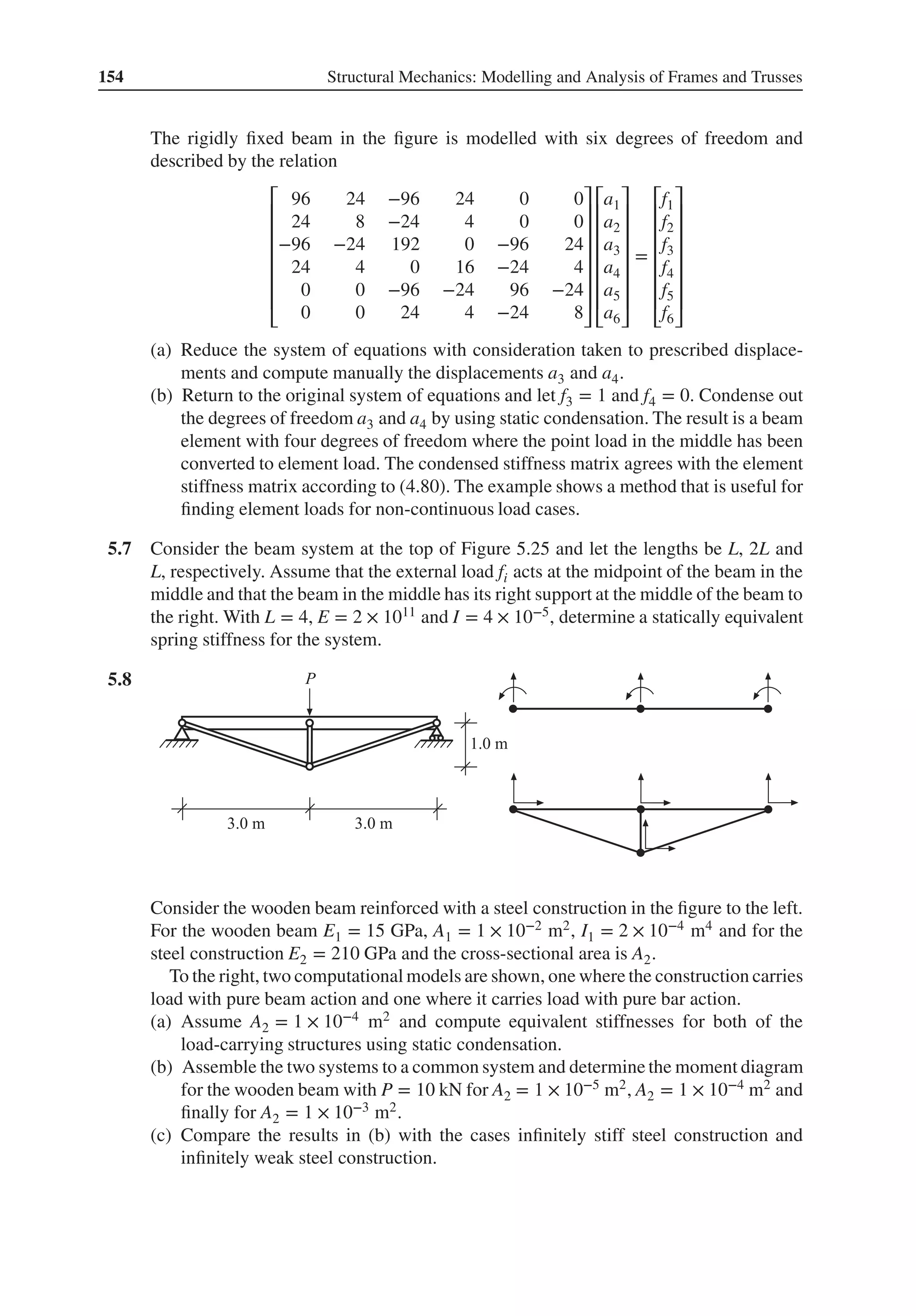
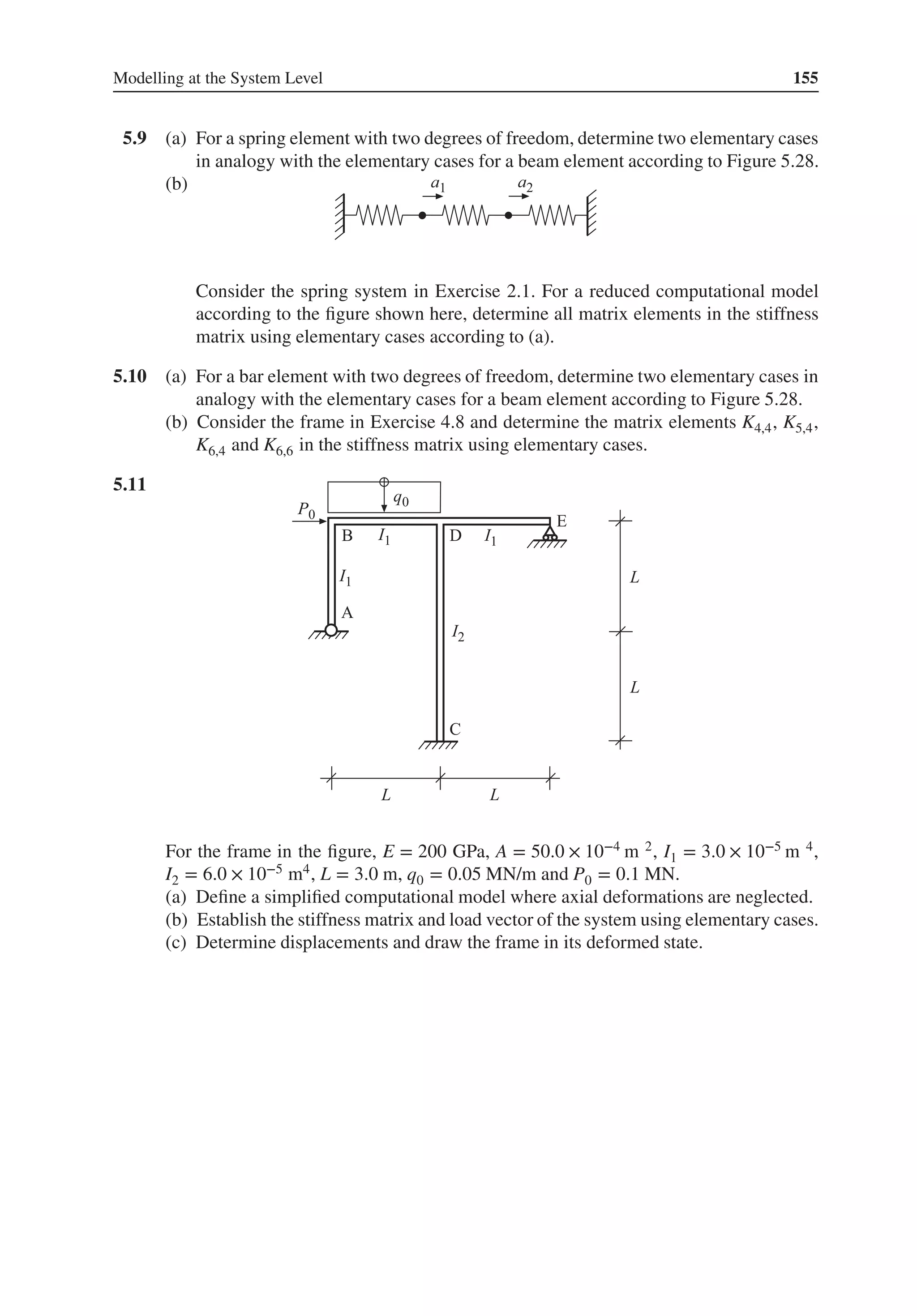

![6
Flexible Supports
Figure 6.1 Flexible supports
A structurecan be supportedby its surroundingsin differentmanners.So far,we have modelled
supports by prescribing displacements of the nodes. This approach allows only for two dif-
ferent options – completely fixed or completely free to move. We here study the possibility
to model deformable supports, which we refer to as flexible supports (Figure 6.1). Flexible
supports can exist both at nodes and along elements.
6.1 Flexible Supports at Nodes
The simplest type of flexible supports is obtained by introducing discrete elastic springs at the
nodes of the structure. From Chapter 2, we have the element relation for a spring:
Ke
ae
= fe
(6.1)
where
Ke
= k
[
1 −1
−1 1
]
; ae
=
[
u1
u2
]
; fe
=
[
P1
P2
]
(6.2)
The element displacements ae can be translation as well as rotational degrees of freedom, as
shown in Figure 6.2.
Structural Mechanics: Modelling and Analysis of Frames and Trusses, First Edition.
Karl-Gunnar Olsson and Ola Dahlblom.
© 2016 John Wiley & Sons, Ltd. Published 2016 by John Wiley & Sons, Ltd.](https://image.slidesharecdn.com/structuralmechanicsmodellingandanalysisofframesandtrussespdfdrive-230720064114-5e1f9a93/75/Structural-mechanics-_-modelling-and-analysis-of-frames-and-trusses-PDFDrive-pdf-171-2048.jpg)
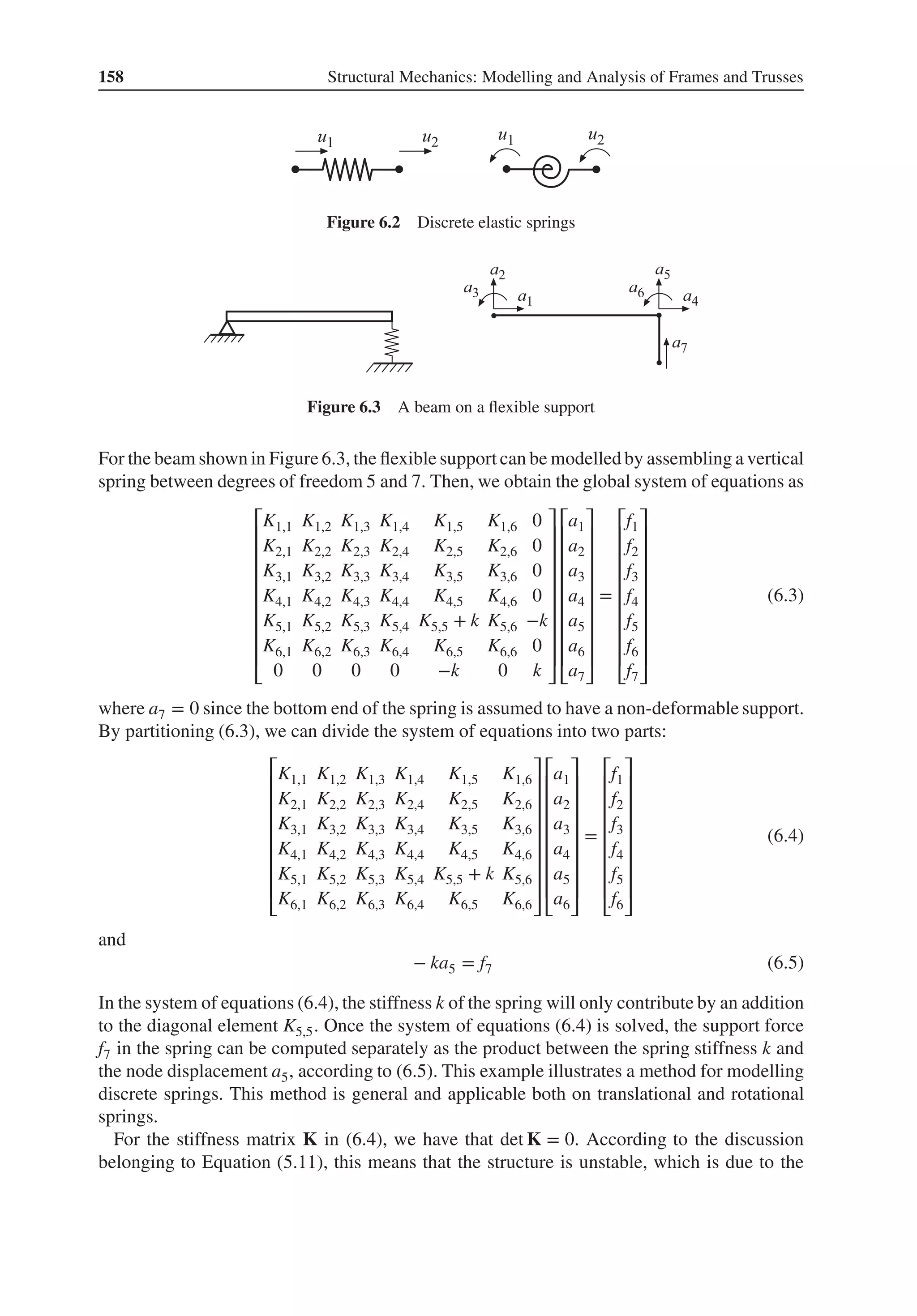
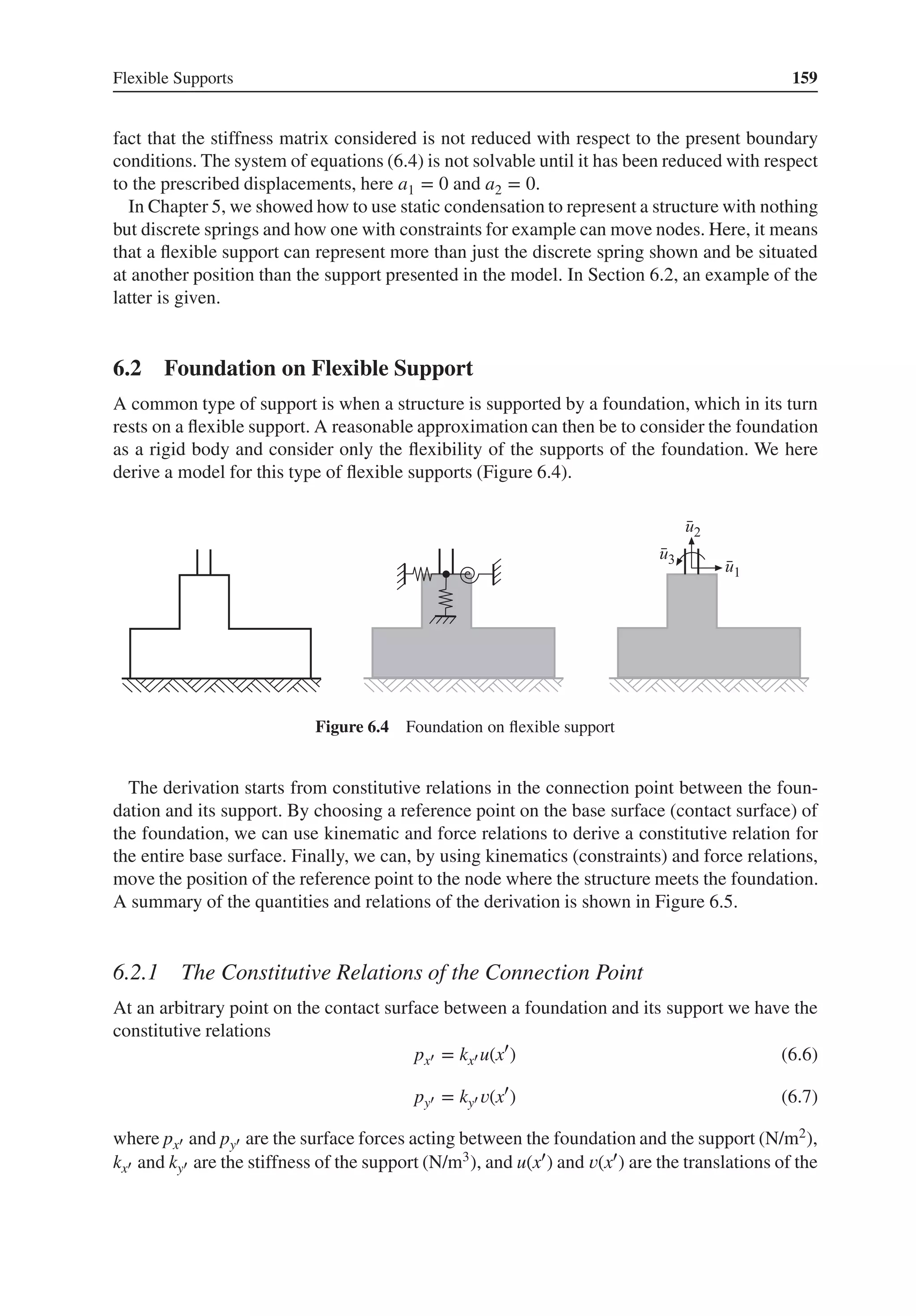
![160 Structural Mechanics: Modelling and Analysis of Frames and Trusses
Figure 6.5 From connection point to foundation
Figure 6.6 The stiffness of the connection point
point [m] horizontally and vertically (Figure 6.6). The relations (6.6) and (6.7) can be written
in matrix form as [
px′
py′
]
=
[
kx′ 0
0 ky′
] [
u(x′)
𝑣(x′)
]
(6.8)](https://image.slidesharecdn.com/structuralmechanicsmodellingandanalysisofframesandtrussespdfdrive-230720064114-5e1f9a93/75/Structural-mechanics-_-modelling-and-analysis-of-frames-and-trusses-PDFDrive-pdf-174-2048.jpg)
![Flexible Supports 161
x'
x'
'
u'
u' u'
z'
y'
y'
Figure 6.7 The local coordinate system, degrees of freedom and associated stiffnesses of the contact
surface
6.2.2 The Constitutive Relation of the Base Surface
To be able to formulate a comprehensive constitutive relation for the entire base surface of
the foundation, we have to choose a reference point. This reference point becomes the ori-
gin for a local coordinate system (x′, y′, z′) (Figure 6.7). We restrict ourselves to discuss
only two-dimensional motion of the foundation and for this we introduce three displacement
degrees of freedom u′
1
, u′
2
and u′
3
at the reference point. With that we have created the required
conditions to establish a stiffness matrix K′e
, which summarises the stiffness of the flexible
support of the base surface.
Kinematics
x' x'
x'u'
x'
x' u'
u' u'
u' u'
Figure 6.8 The kinematics of the base surface
For a rigid body motion of the foundation, the following kinematic relations between the
displacements of the reference point and an arbitrary point on the base surface (Figure 6.8)
can be established as
u(x′
) = u′
1 (6.9)
𝑣(x′
) = u′
2 + x′
u′
3 (6.10)
or in matrix form as
[
u(x′)
𝑣(x′)
]
=
[
1 0 0
0 1 x′
] ⎡
⎢
⎢
⎢
⎣
u′
1
u′
2
u′
3
⎤
⎥
⎥
⎥
⎦
(6.11)](https://image.slidesharecdn.com/structuralmechanicsmodellingandanalysisofframesandtrussespdfdrive-230720064114-5e1f9a93/75/Structural-mechanics-_-modelling-and-analysis-of-frames-and-trusses-PDFDrive-pdf-175-2048.jpg)
![162 Structural Mechanics: Modelling and Analysis of Frames and Trusses
Force Relations
P'
P'
P'
px'
x'
py'
Figure 6.9 Resulting forces
If we consider the foundation in its original state, the resulting forces acting on the support at
the reference point of the base surface (Figure 6.9) are obtained as
P′
1 =
∫A
px′ dA (6.12)
P′
2 =
∫A
py′ dA (6.13)
P′
3 =
∫A
x′
py′ dA (6.14)
or in matrix form as
⎡
⎢
⎢
⎢
⎣
P′
1
P′
2
P′
3
⎤
⎥
⎥
⎥
⎦
=
∫A
⎡
⎢
⎢
⎣
1 0
0 1
0 x′
⎤
⎥
⎥
⎦
[
px′
py′
]
dA (6.15)
Constitutive Relation
Substituting (6.8) and (6.11) into (6.15) and keeping in mind that the displacements u′
1
, u′
2
and
u′
3
are quantities that remain unchanged across the cross-section and, therefore, can be moved
outside the integral, we obtain
K′e
a′e
= f′e
(6.16)
where
K′e
=
⎡
⎢
⎢
⎢
⎣
∫Akx′ dA 0 0
0 ∫Aky′ dA ∫Ax′ky′ dA
0 ∫Ax′ky′ dA ∫Ax′2
ky′ dA
⎤
⎥
⎥
⎥
⎦
; a′e
=
⎡
⎢
⎢
⎢
⎣
u′
1
u′
2
u′
3
⎤
⎥
⎥
⎥
⎦
; f′e
=
⎡
⎢
⎢
⎢
⎣
P′
1
P′
2
P′
3
⎤
⎥
⎥
⎥
⎦
(6.17)](https://image.slidesharecdn.com/structuralmechanicsmodellingandanalysisofframesandtrussespdfdrive-230720064114-5e1f9a93/75/Structural-mechanics-_-modelling-and-analysis-of-frames-and-trusses-PDFDrive-pdf-176-2048.jpg)
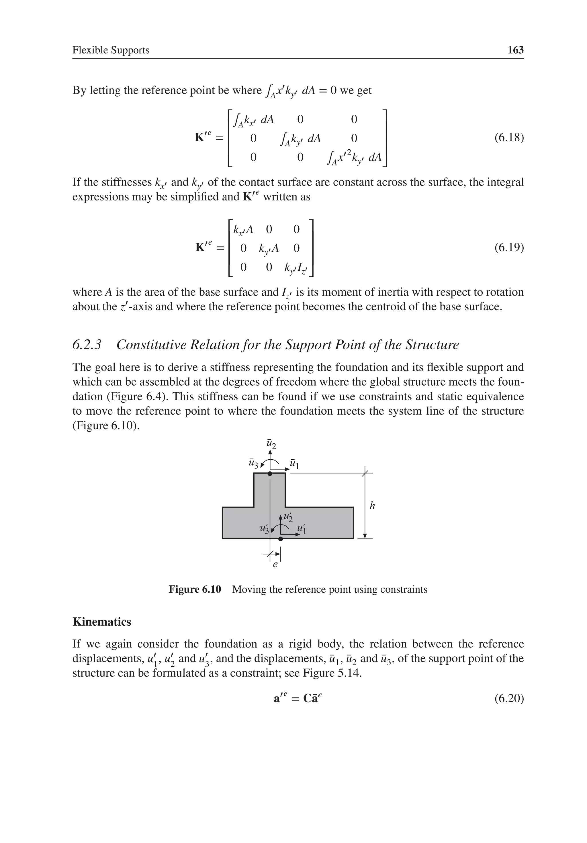
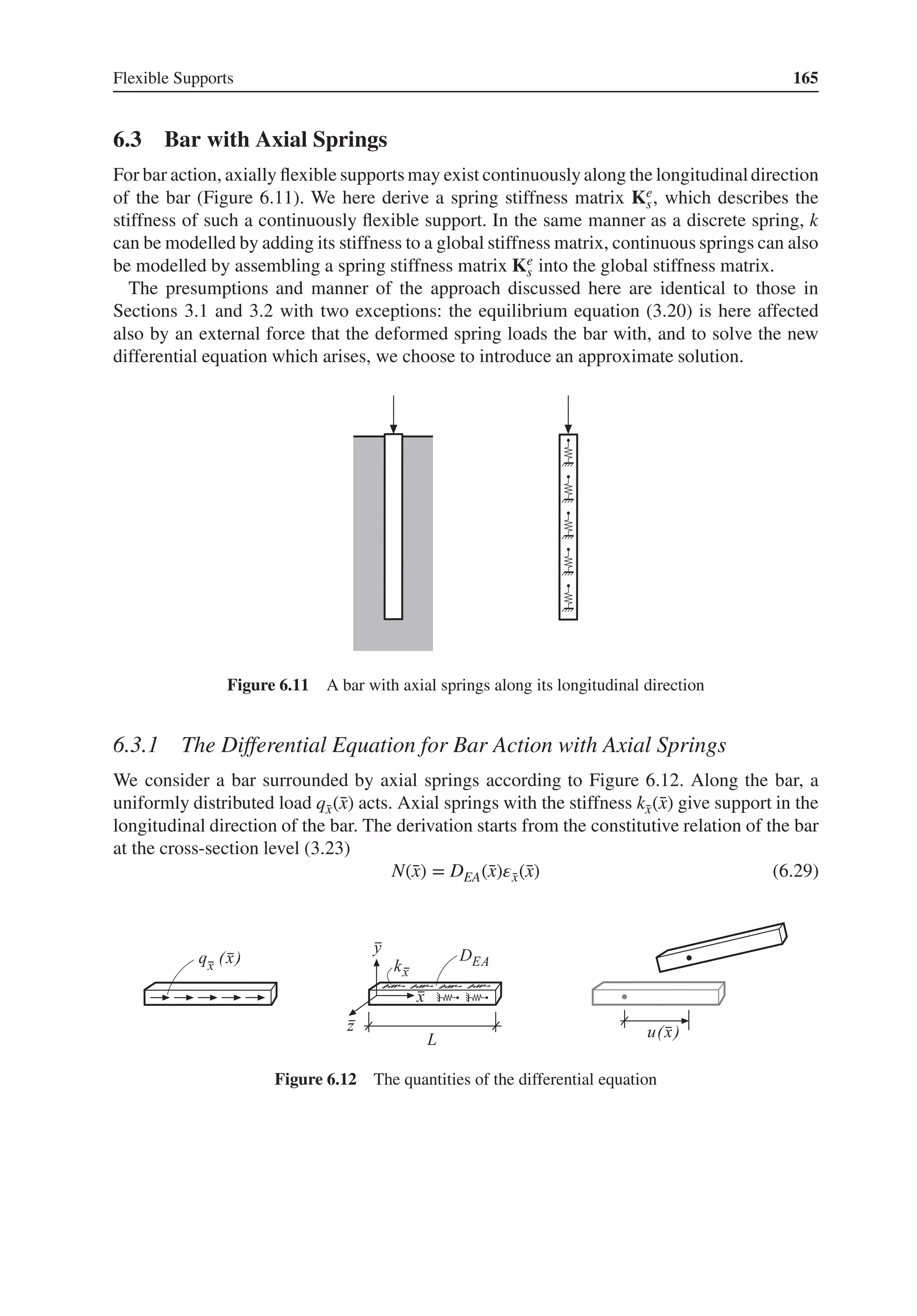
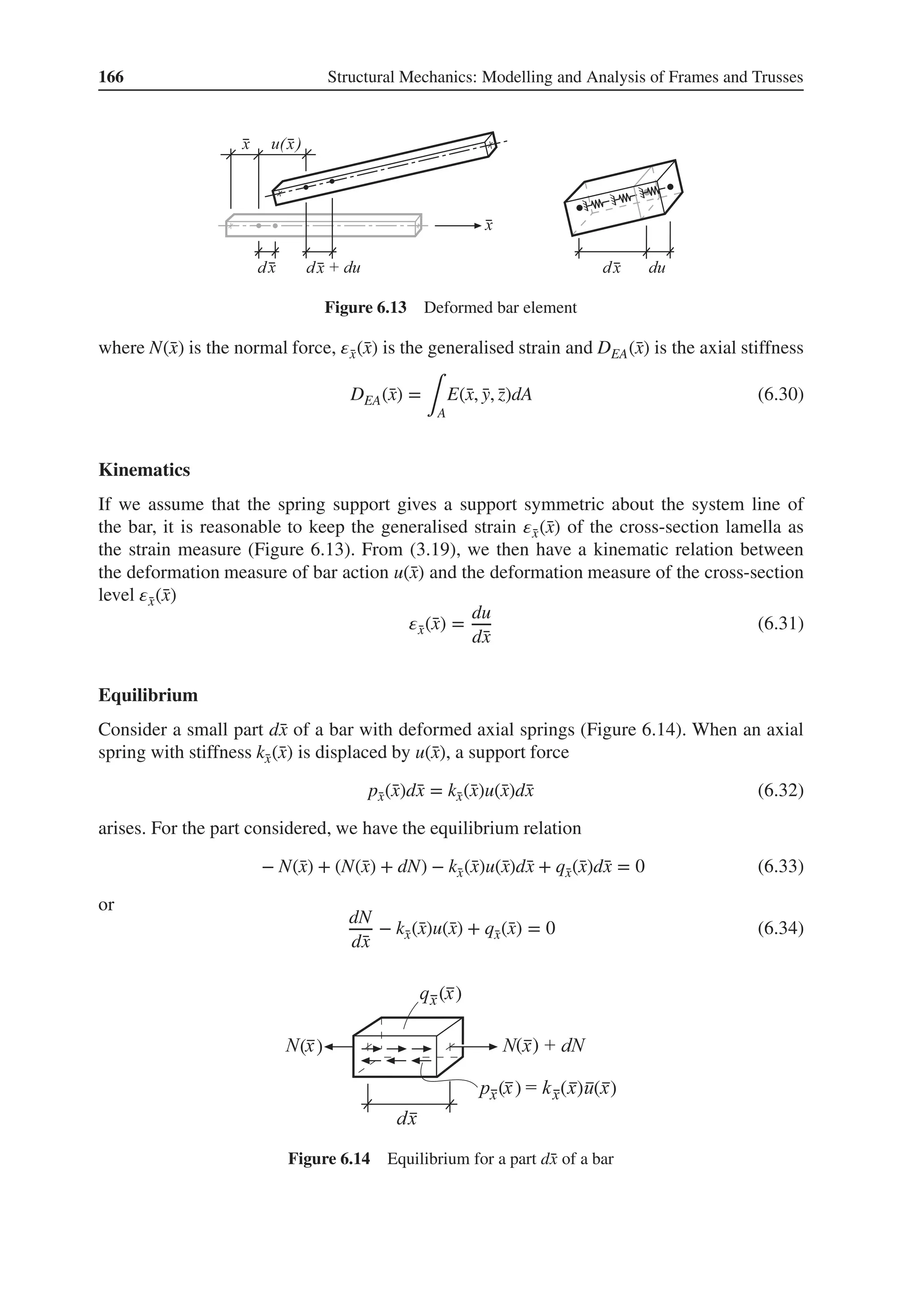
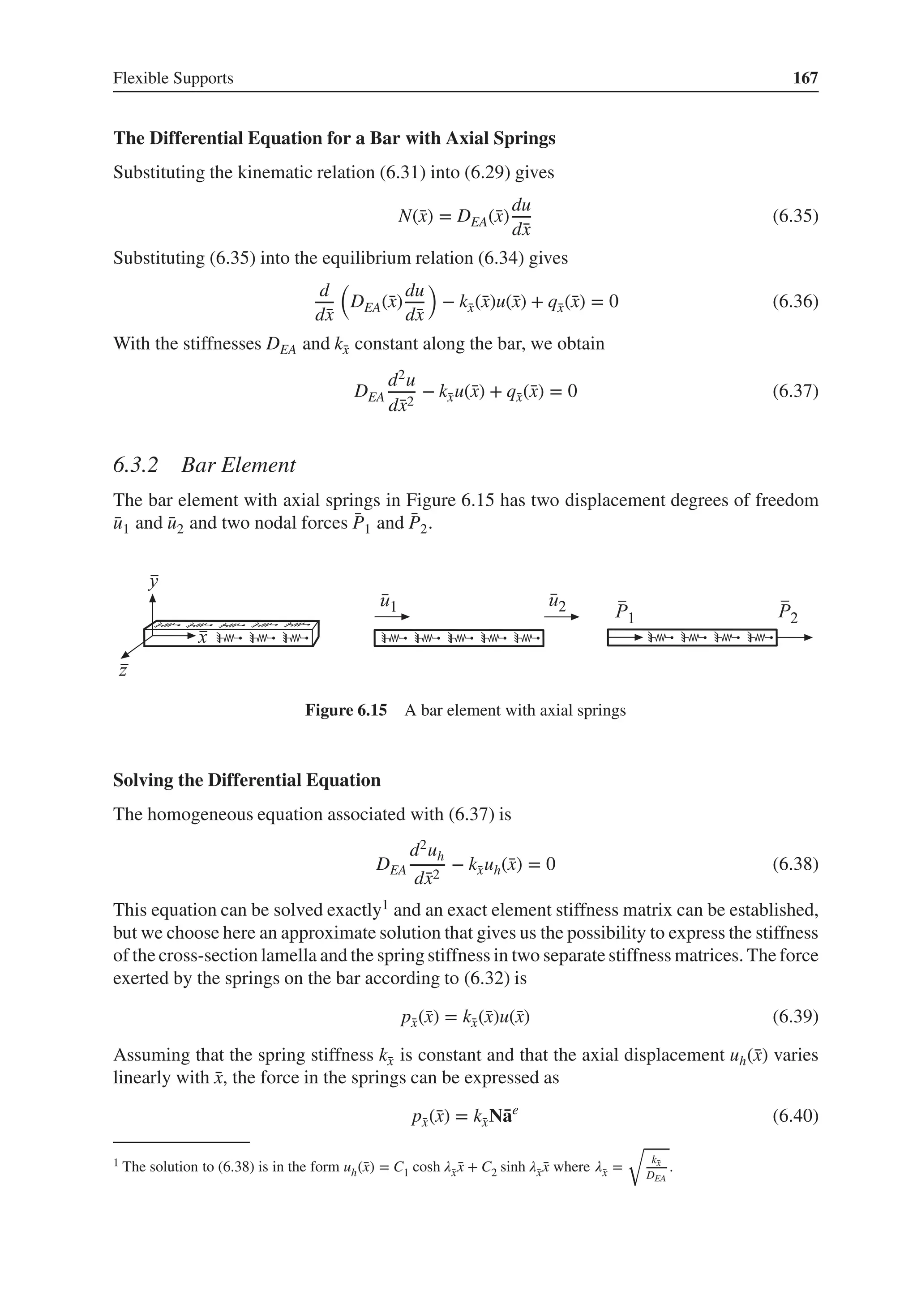
![168 Structural Mechanics: Modelling and Analysis of Frames and Trusses
where N̄
ae is the displacement of a bar element without springs and without axial load, accord-
ing to Chapter 3. The differential equation (6.37) can, when we use the approximation (6.40),
be written as
DEA
d2u
d̄
x2
− p̄
x(̄
x) + q̄
x(̄
x) = 0 (6.41)
and the homogeneous equation associated with this equation is
DEA
d2uh
d̄
x2
= 0 (6.42)
As we have seen in Chapter 3, the solution to (6.42) is given by (3.41), that is
uh(̄
x) = N̄
ae
(6.43)
where according to (3.42) and (3.38)
N = ̄
NC−1
=
[
1 ̄
x
]
[
1 0
−1
L
1
L
]
=
[
1 − ̄
x
L
̄
x
L
]
; ̄
ae
=
[
̄
u1
̄
u2
]
(6.44)
Differentiation of (6.43) gives
duh
d̄
x
=
[
0 1
]
[
1 0
−1
L
1
L
]
[
̄
u1
̄
u2
]
=
[
−1
L
1
L
][
̄
u1
̄
u2
]
(6.45)
The general solution to (6.41) can be written as
u(̄
x) = uh(̄
x) + up(̄
x) (6.46)
The particular solution is obtained by twice integrating (6.41) with (6.40) substituted. For the
case with a constant load q̄
x, we obtain
up(̄
x) =
k̄
x
DEA
[
̄
x2
2
̄
x3
6
][
1 0
−1
L
1
L
][
̄
u1
̄
u2
]
+
1
DEA
(
−q̄
x
̄
x2
2
+ C1 ̄
x + C2
)
(6.47)
The boundary conditions (3.47) and (3.48) give
C2 = 0 (6.48)
C1 = −k̄
x
[
L
2
L2
6
][
1 0
−1
L
1
L
][
̄
u1
̄
u2
]
+ q̄
x
L
2
(6.49)
that is
up(̄
x) =
k̄
x
DEA
[
̄
x2−L̄
x
2
̄
x3−L2 ̄
x
6
][
1 0
−1
L
1
L
][
̄
u1
̄
u2
]
−
q̄
x
DEA
(
̄
x2
2
−
L̄
x
2
)
(6.50)
Differentiation gives
dup
d̄
x
=
k̄
x
DEA
[
2̄
x−L
2
3̄
x2−L2
6
]
[
1 0
−1
L
1
L
][
̄
u1
̄
u2
]
−
q̄
x
DEA
(
̄
x −
L
2
)
(6.51)](https://image.slidesharecdn.com/structuralmechanicsmodellingandanalysisofframesandtrussespdfdrive-230720064114-5e1f9a93/75/Structural-mechanics-_-modelling-and-analysis-of-frames-and-trusses-PDFDrive-pdf-182-2048.jpg)
![Flexible Supports 169
or
dup
d̄
x
=
k̄
x
DEA
[
− ̄
x2
2L
+ ̄
x − L
3
̄
x2
2L
− L
6
][
̄
u1
̄
u2
]
−
q̄
x
DEA
(
̄
x −
L
2
)
(6.52)
An expression for the normal force N(̄
x) can be determined by substituting (6.46), (6.45) and
(6.52) into (6.35)
N(̄
x) = DEA
[
−1
L
1
L
]
[
̄
u1
̄
u2
]
+k̄
x
[
− ̄
x2
2L
+ ̄
x − L
3
̄
x2
2L
− L
6
]
[
̄
u1
̄
u2
]
−q̄
x
(
̄
x −
L
2
)
(6.53)
For ̄
x = 0 and ̄
x = L, we have
̄
P1 = −N(0) = DEA
[
1
L
−1
L
]
[
̄
u1
̄
u2
]
+ k̄
x
[
L
3
L
6
][
̄
u1
̄
u2
]
− q̄
x
L
2
(6.54)
̄
P2 = N(L) = DEA
[
−1
L
1
L
]
[
̄
u1
̄
u2
]
+ k̄
x
[
L
6
L
3
][
̄
u1
̄
u2
]
− q̄
x
L
2
(6.55)
or
̄
Ke
̄
ae
= ̄
fe
(6.56)
where
̄
Ke
= ̄
Ke
0 + ̄
Ke
s; ̄
fe
= ̄
fe
b + ̄
fe
l (6.57)
̄
Ke
0 =
DEA
L
[
1 −1
−1 1
]
; ̄
Ke
s = k̄
xL
⎡
⎢
⎢
⎣
1
3
1
6
1
6
1
3
⎤
⎥
⎥
⎦
(6.58)
̄
ae
=
[
̄
u1
̄
u2
]
; ̄
fe
b =
[
̄
P1
̄
P2
]
; ̄
fe
l =
q̄
xL
2
[
1
1
]
(6.59)
Equation (6.56) formulates the element relations for a bar with axial springs. The element
stiffness matrix here consists of two parts: one matrix ̄
Ke
0
describing the stiffness of a bar
without springs and a matrix ̄
Ke
s describing the stiffness of the springs.
Example 6.1 Choice of element length for a bar with axial springs
Figure 1 A bar with axial springs](https://image.slidesharecdn.com/structuralmechanicsmodellingandanalysisofframesandtrussespdfdrive-230720064114-5e1f9a93/75/Structural-mechanics-_-modelling-and-analysis-of-frames-and-trusses-PDFDrive-pdf-183-2048.jpg)
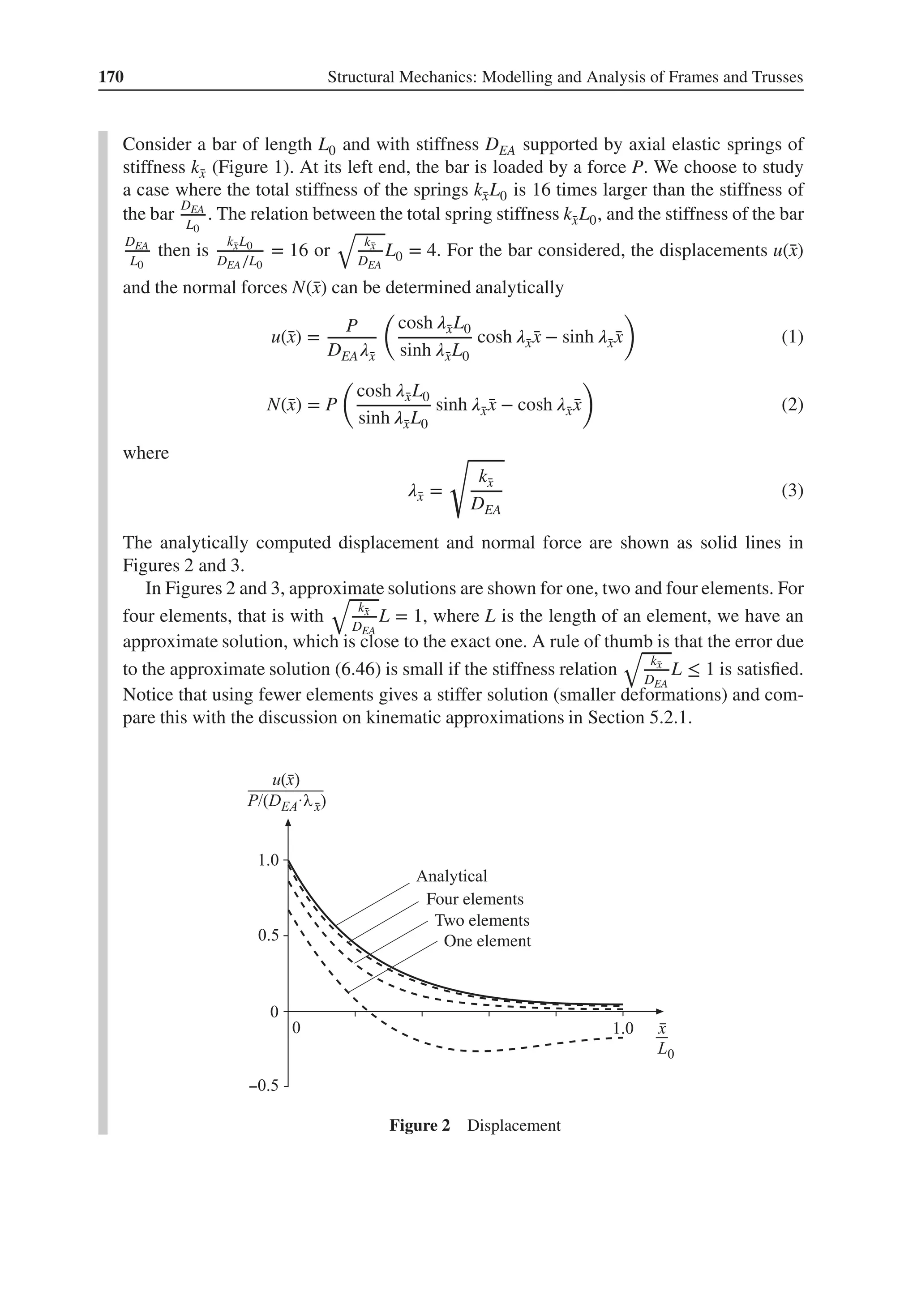
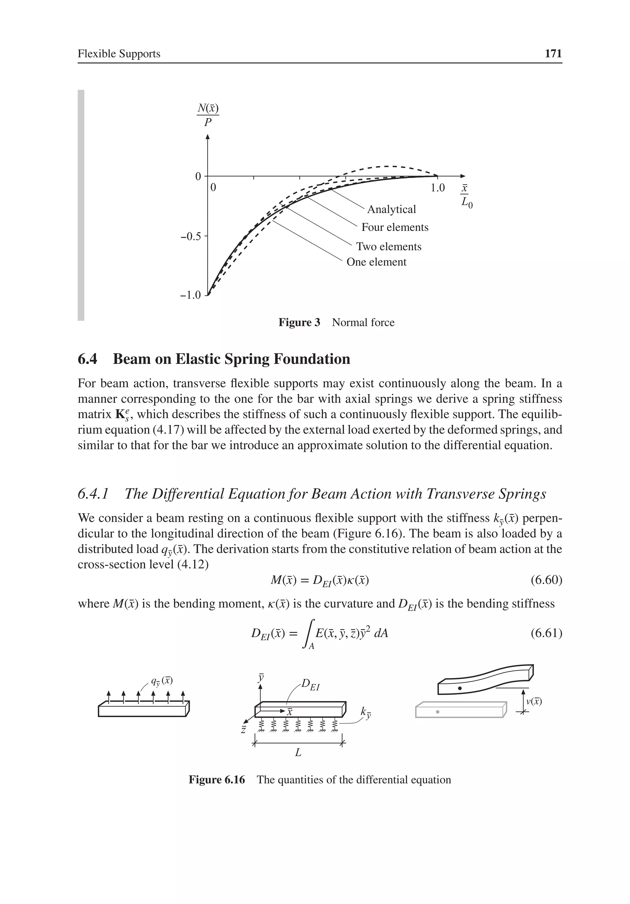
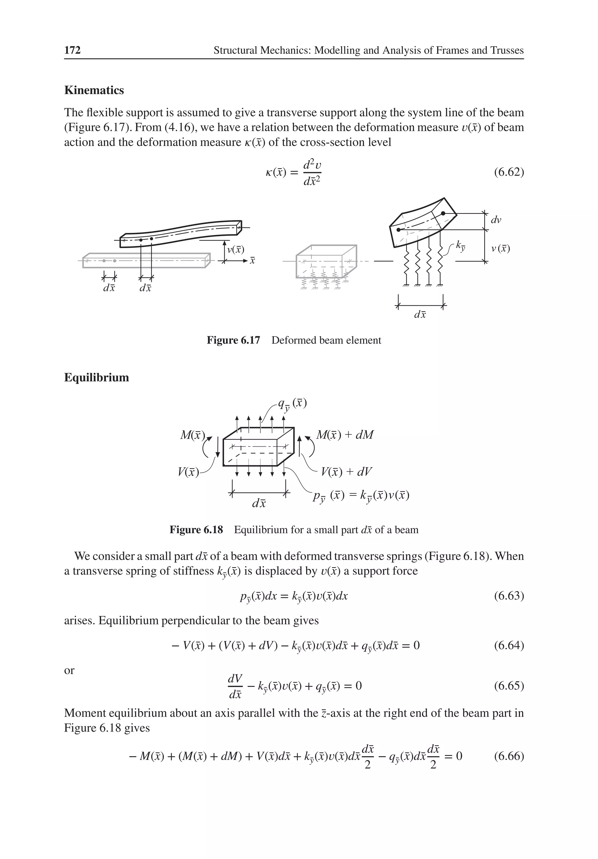
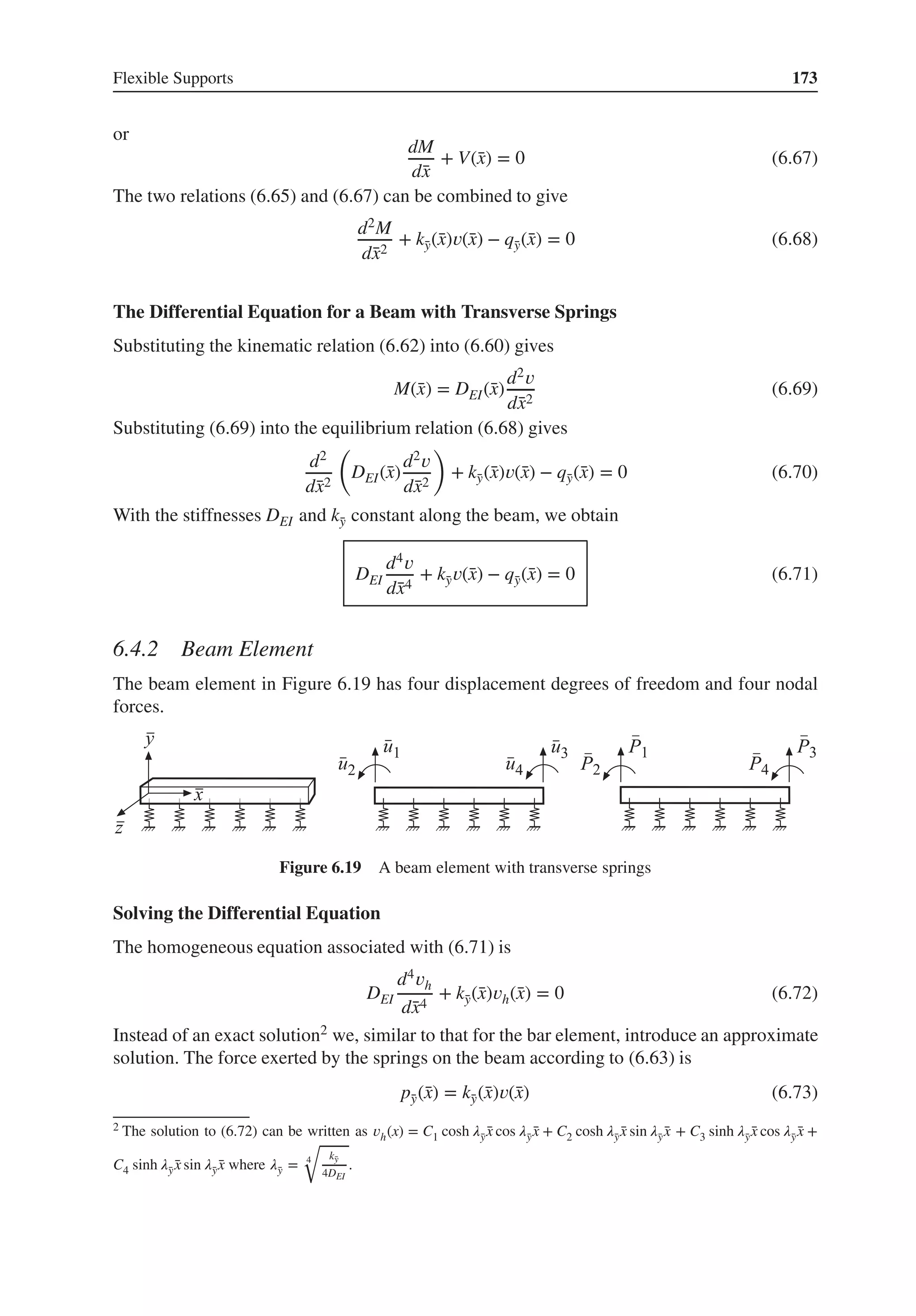
![174 Structural Mechanics: Modelling and Analysis of Frames and Trusses
Assuming that the spring stiffness k̄
y is constant and that the transverse displacement can be
described by a polynomial of degree three, the force in the springs can be expressed as
p̄
y(̄
x) = k̄
yN̄
ae
(6.74)
where N̄
ae is the displacement of a beam element without springs and without transverse load,
according to Chapter 4. The differential equation (6.71), using the approximation (6.74), can
be written as
DEI
d4𝑣
d̄
x4
+ p̄
y(̄
x) − q̄
y(̄
x) = 0 (6.75)
and the homogeneous equation associated with this differential equation is
DEI
d4𝑣h
d̄
x4
= 0 (6.76)
The solution to (6.76) is given from (4.47) of Chapter 4,
𝑣h(̄
x) = N̄
ae
(6.77)
where
N = ̄
NC−1
=
[
1 ̄
x ̄
x2 ̄
x3
]
⎡
⎢
⎢
⎢
⎢
⎣
1 0 0 0
0 1 0 0
− 3
L2 −2
L
3
L2 −1
L
2
L3
1
L2 − 2
L3
1
L2
⎤
⎥
⎥
⎥
⎥
⎦
; ̄
ae
=
⎡
⎢
⎢
⎢
⎢
⎣
̄
u1
̄
u2
̄
u3
̄
u4
⎤
⎥
⎥
⎥
⎥
⎦
(6.78)
Differentiating (6.77) gives
d2𝑣h
d̄
x2
= B̄
ae
(6.79)
d3𝑣h
d̄
x3
=
dB
d̄
x
̄
ae
(6.80)
where
B =
d2N
d̄
x2
=
d2 ̄
N
d̄
x2
C−1
=
[
0 0 2 6̄
x
]
⎡
⎢
⎢
⎢
⎢
⎣
1 0 0 0
0 1 0 0
− 3
L2 −2
L
3
L2 −1
L
2
L3
1
L2 − 2
L3
1
L2
⎤
⎥
⎥
⎥
⎥
⎦
(6.81)
dB
d̄
x
=
d3N
d̄
x3
=
d3 ̄
N
d̄
x3
C−1
=
[
0 0 0 6
]
⎡
⎢
⎢
⎢
⎢
⎣
1 0 0 0
0 1 0 0
− 3
L2 −2
L
3
L2 −1
L
2
L3
1
L2 − 2
L3
1
L2
⎤
⎥
⎥
⎥
⎥
⎦
(6.82)](https://image.slidesharecdn.com/structuralmechanicsmodellingandanalysisofframesandtrussespdfdrive-230720064114-5e1f9a93/75/Structural-mechanics-_-modelling-and-analysis-of-frames-and-trusses-PDFDrive-pdf-188-2048.jpg)
![Flexible Supports 175
The general solution to (6.75) can be written as
𝑣(̄
x) = 𝑣h(̄
x) + 𝑣p(̄
x) (6.83)
The particular solution is obtained by integrating (6.75) four times with (6.74) substituted. For
the case with a constant load q̄
y, we obtain
𝑣p(̄
x) = −
k̄
y
DEI
[
̄
x4
24
̄
x5
120
̄
x6
360
̄
x7
840
]
C−1
̄
ae
+
1
DEI
(
q̄
y
̄
x4
24
+ C1
̄
x3
6
+ C2
̄
x2
2
+ C3 ̄
x + C4
)
(6.84)
The boundary conditions (4.56)–(4.59) give
C1 = k̄
y
[
L
2
3L2
20
L3
15
L4
28
]
C−1
̄
ae
− q̄
y
L
2
(6.85)
C2 = −k̄
y
[
L2
12
L3
30
L4
60
L5
105
]
C−1
̄
ae
+ q̄
y
L2
12
(6.86)
C3 = 0 (6.87)
C4 = 0 (6.88)
that is
𝑣p(̄
x) = −
k̄
y
DEI
⎡
⎢
⎢
⎢
⎢
⎢
⎢
⎣
̄
x4−2L̄
x3+L2 ̄
x2
24
̄
x5−3L2 ̄
x3+2L3 ̄
x2
120
̄
x6−4L3 ̄
x3+3L4 ̄
x2
360
̄
x7−5L4 ̄
x3+4L5 ̄
x2
840
⎤
⎥
⎥
⎥
⎥
⎥
⎥
⎦
T
C−1
̄
ae
+
q̄
y
DEI
(
̄
x4
24
−
L̄
x3
12
+
L2 ̄
x2
24
)
(6.89)
d2𝑣p
d̄
x2
= −
k̄
y
DEI
⎡
⎢
⎢
⎢
⎢
⎢
⎢
⎣
6̄
x2−6L̄
x+L2
12
10̄
x3−9L2 ̄
x+2L3
60
5̄
x4−4L3 ̄
x+L4
60
21̄
x5−15L4 ̄
x+4L5
420
⎤
⎥
⎥
⎥
⎥
⎥
⎥
⎦
T
C−1
̄
ae
+
q̄
y
DEI
(
̄
x2
2
−
L̄
x
2
+
L2
12
)
(6.90)
d3𝑣p
d̄
x3
= −
k̄
y
DEI
⎡
⎢
⎢
⎢
⎢
⎢
⎢
⎣
2̄
x−L
2
10̄
x2−3L2
20
5̄
x3−L3
15
7̄
x4−L4
28
⎤
⎥
⎥
⎥
⎥
⎥
⎥
⎦
T
C−1
̄
ae
+
q̄
y
DEI
(
̄
x −
L
2
)
(6.91)](https://image.slidesharecdn.com/structuralmechanicsmodellingandanalysisofframesandtrussespdfdrive-230720064114-5e1f9a93/75/Structural-mechanics-_-modelling-and-analysis-of-frames-and-trusses-PDFDrive-pdf-189-2048.jpg)
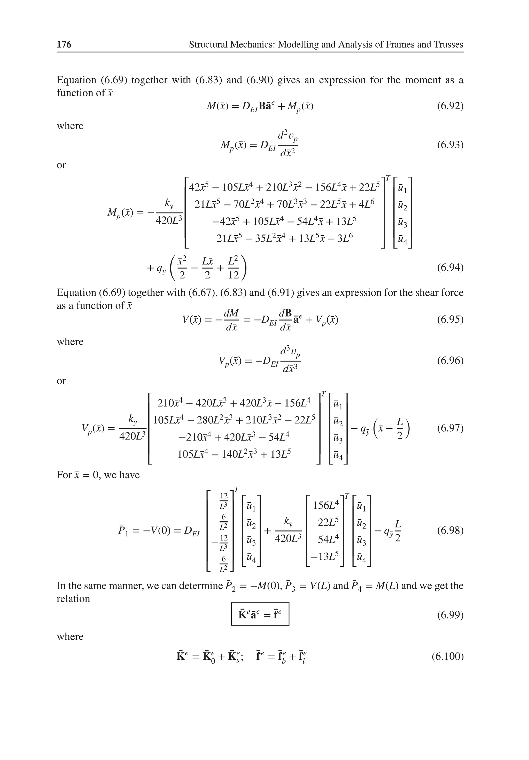
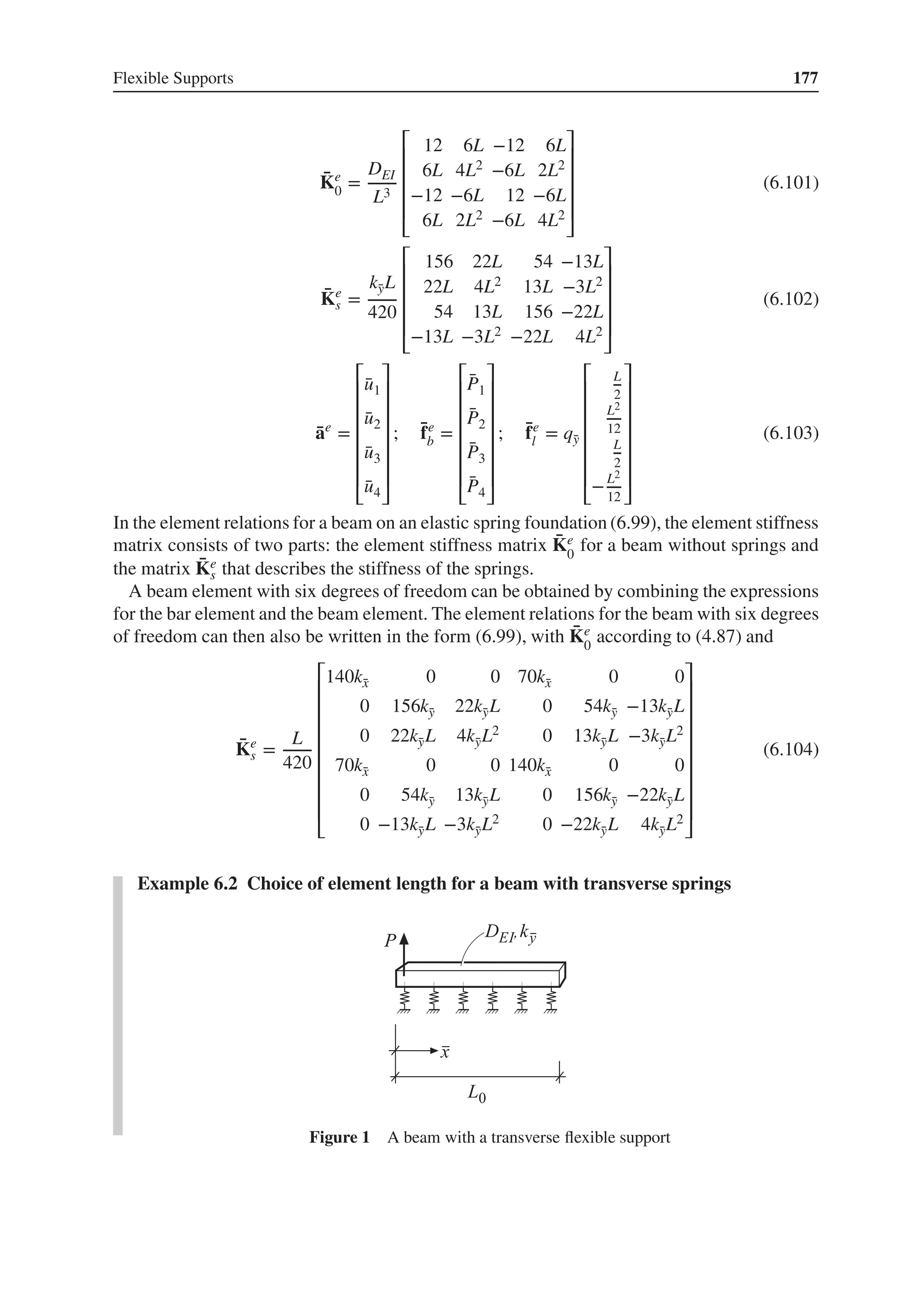
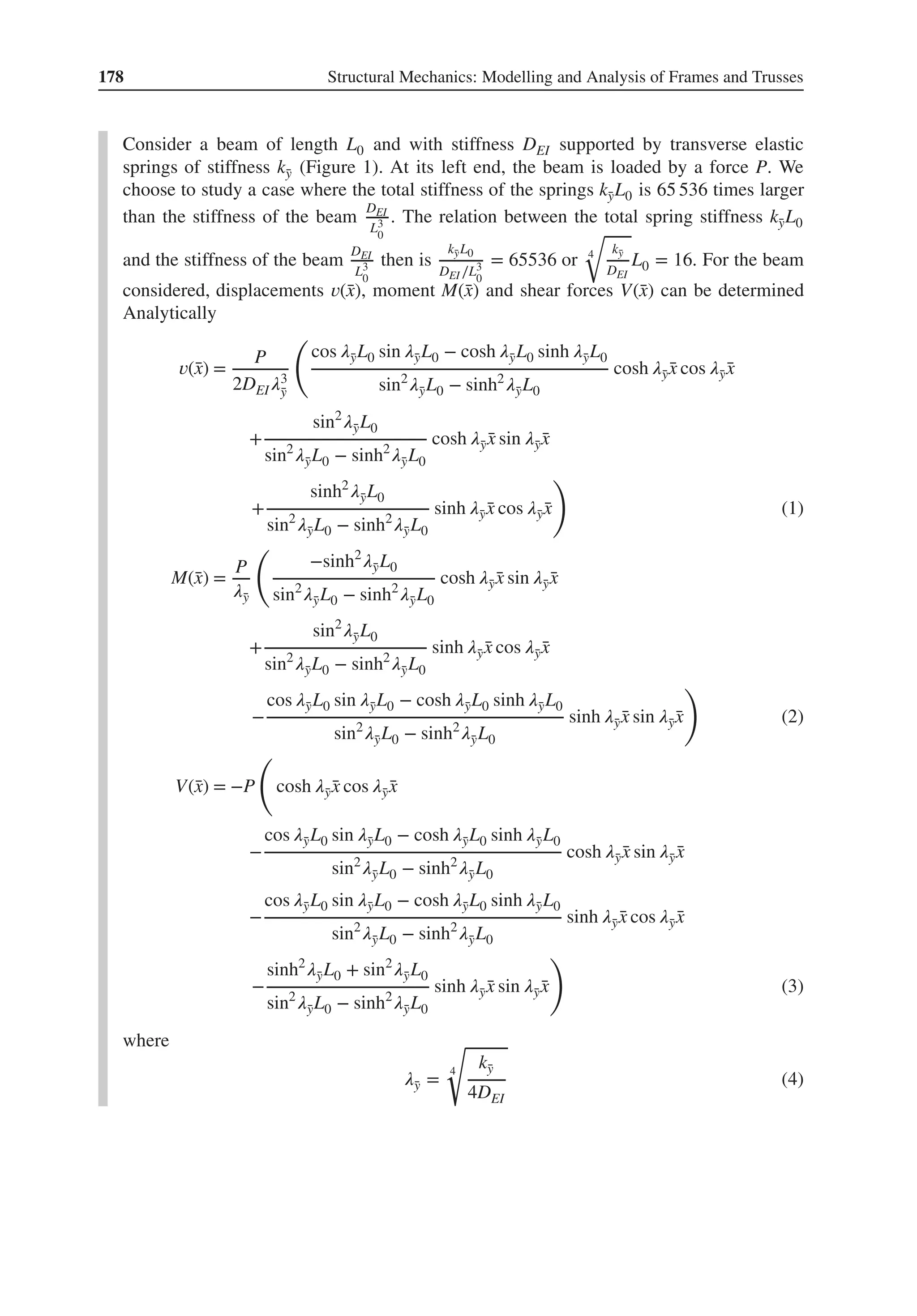
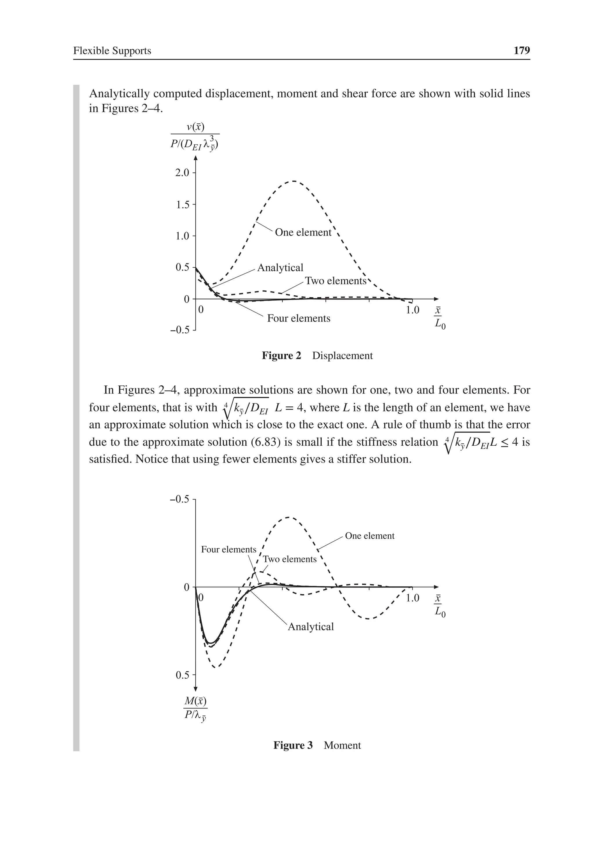

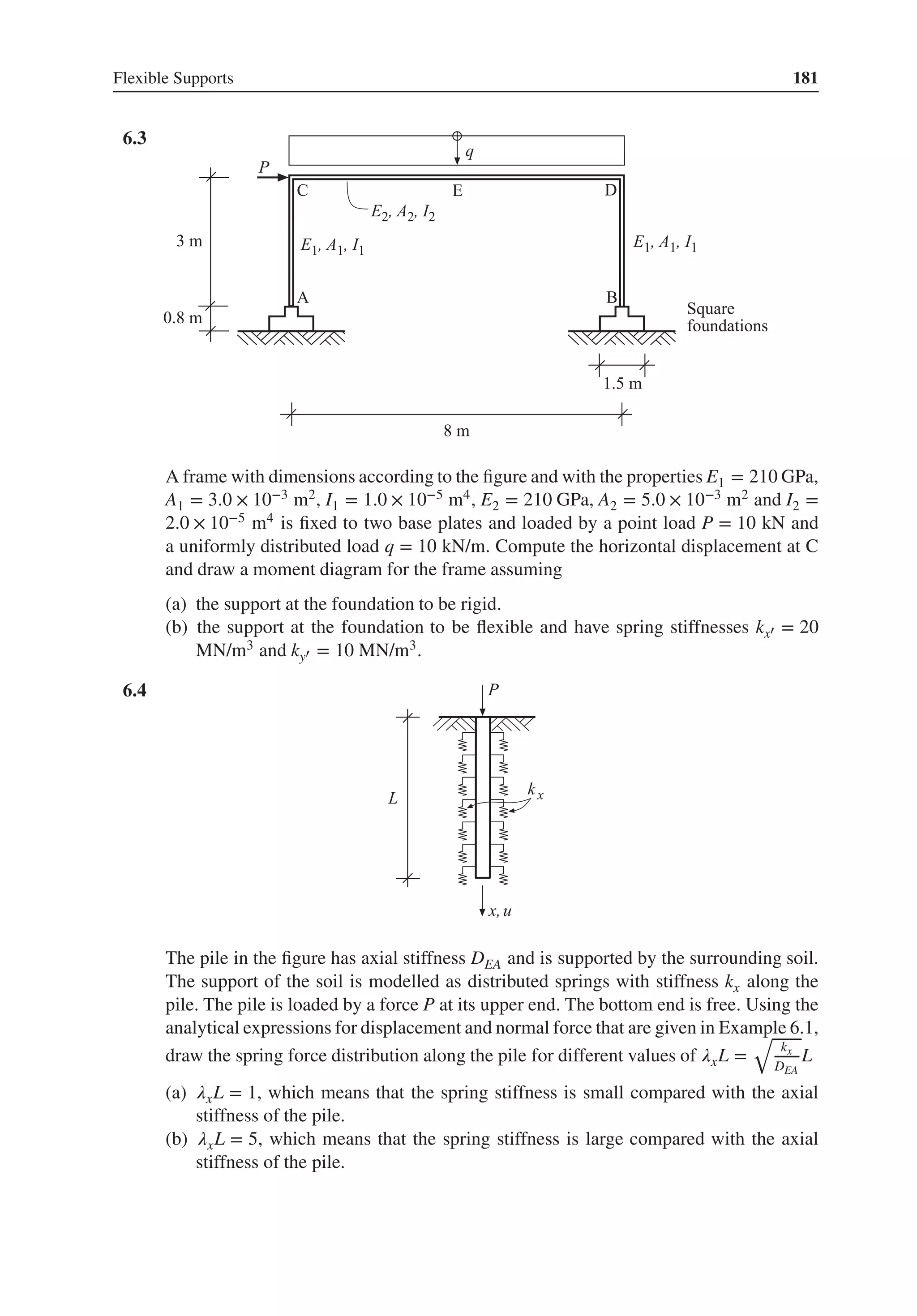
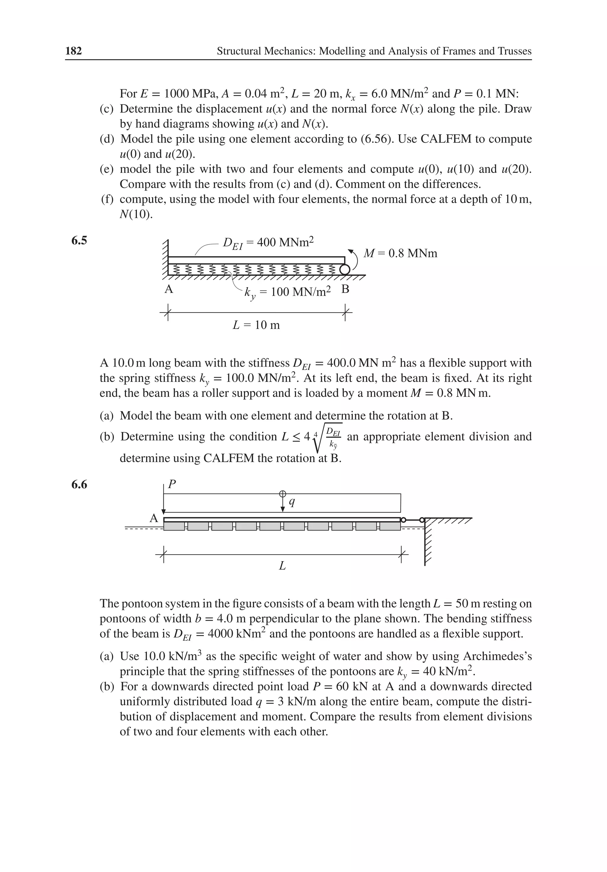
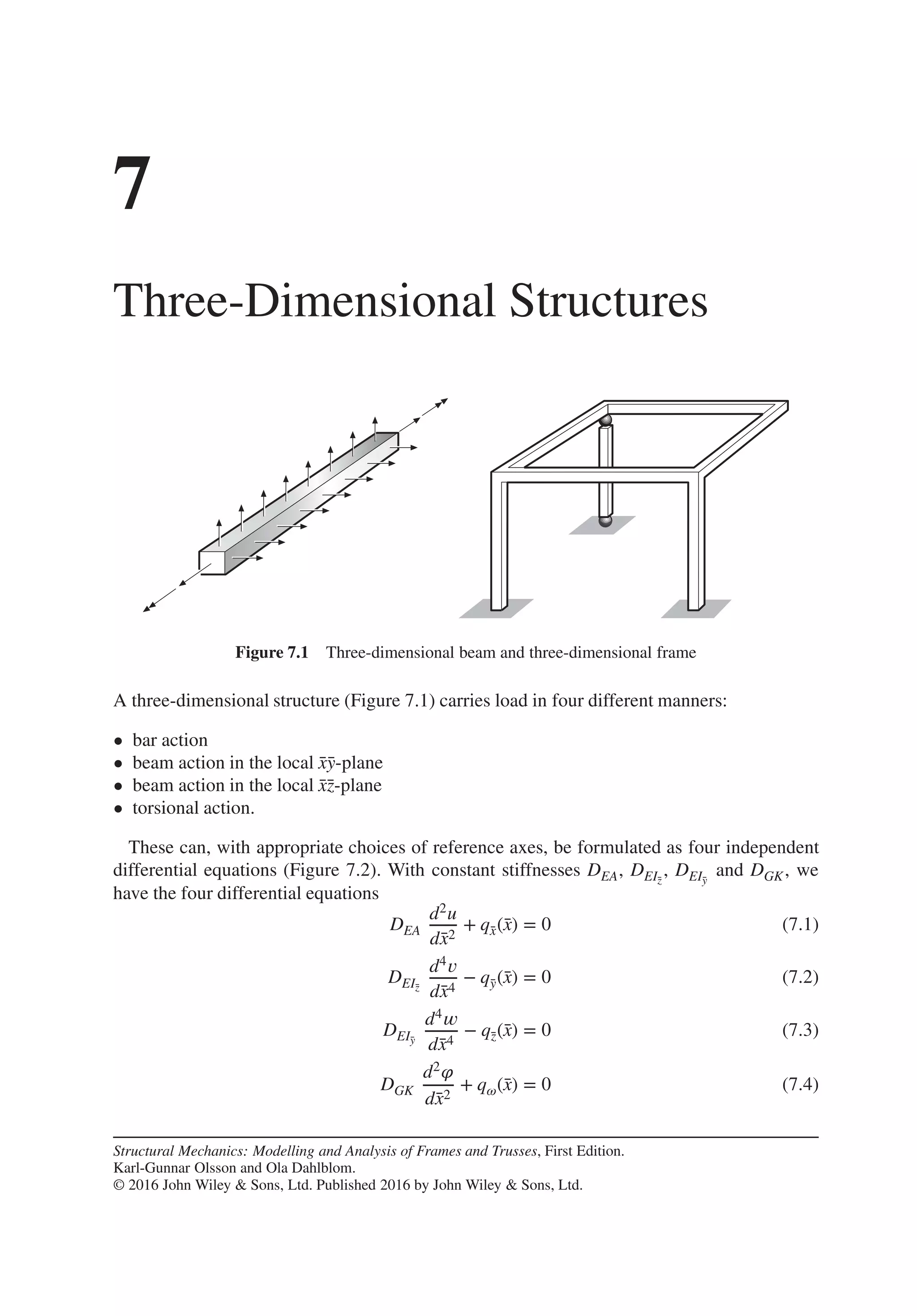
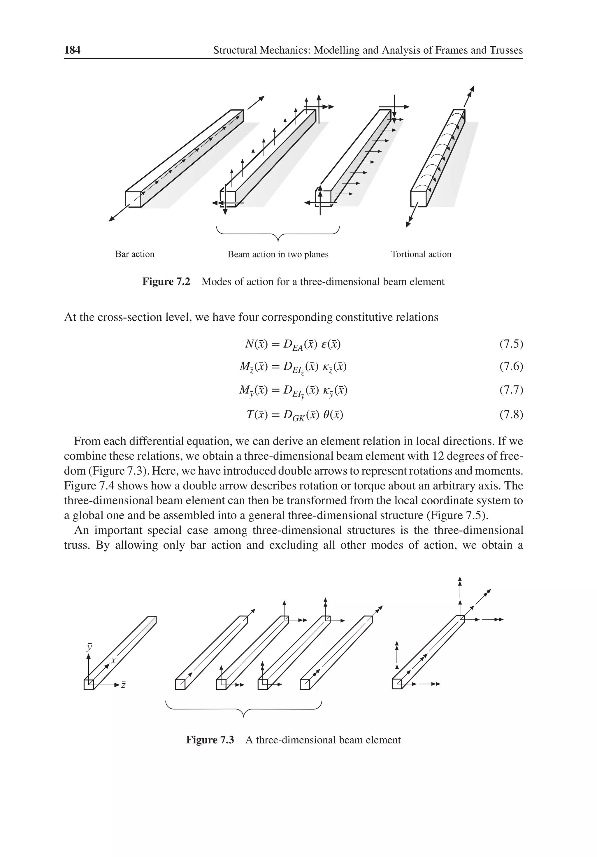
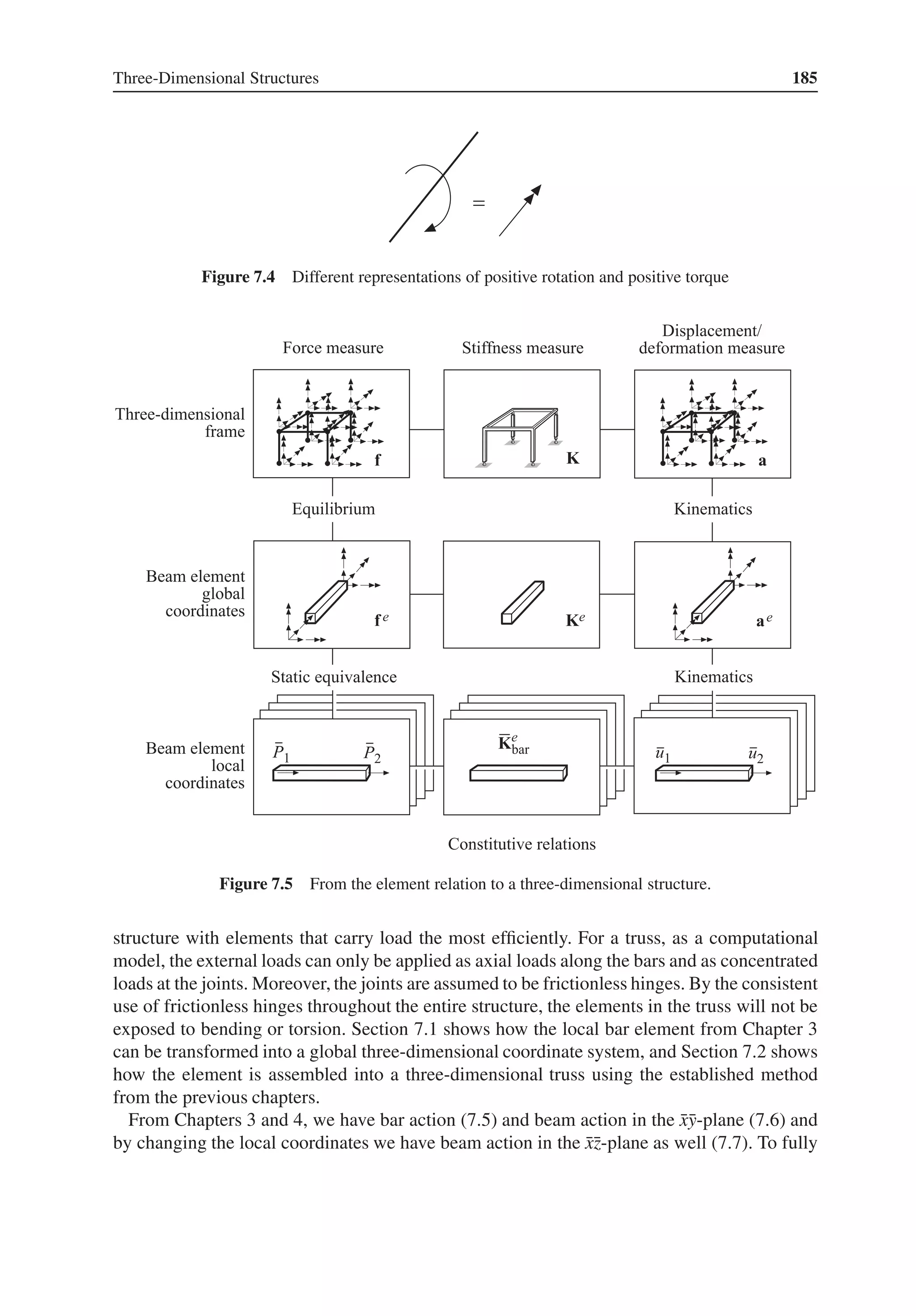
![186 Structural Mechanics: Modelling and Analysis of Frames and Trusses
establish the three-dimensional beam, we must add torsional action. In Section 7.3, a consti-
tutive relation at the cross-section level (7.8) and the differential equation for torsional action
(7.4) are derived. In Section 7.4, the element relations for the three-dimensional beam element
are formulated. Finally, Section 7.5 shows how a computational model for a three-dimensional
frame is established.
7.1 Three-Dimensional Bar Element
To be able to place the bar element (3.60) in a three-dimensional truss, we have to use forces
and displacements in the global coordinate system (x, y, z) of the truss. Here, the displacements
of the bar are described by the displacement components u1, u2, u3, u4, u5 and u6 and its nodal
forces by the force components P1, P2, P3, P4, P5 and P6 (Figure 7.6).
By using direction cosines, analogous to (3.73) and (3.74), the displacements ̄
u1 and ̄
u2 in
the longitudinal direction of the bar can be expressed in the global displacement components
u1, u2, u3, u4 u5 and u6 according to
̄
u1 = nx̄
xu1 + nȳ
xu2 + nz̄
xu3 (7.9)
̄
u2 = nx̄
xu4 + nȳ
xu5 + nz̄
xu6 (7.10)
or in matrix form
̄
ae
= Gae
(7.11)
where
̄
ae
=
[
̄
u1
̄
u2
]
; G =
[
nx̄
x nȳ
x nz̄
x 0 0 0
0 0 0 nx̄
x nȳ
x nz̄
x
]
; ae
=
⎡
⎢
⎢
⎢
⎢
⎢
⎢
⎣
u1
u2
u3
u4
u5
u6
⎤
⎥
⎥
⎥
⎥
⎥
⎥
⎦
(7.12)
Figure 7.6 Three-dimensional bar element with local and global degrees of freedom](https://image.slidesharecdn.com/structuralmechanicsmodellingandanalysisofframesandtrussespdfdrive-230720064114-5e1f9a93/75/Structural-mechanics-_-modelling-and-analysis-of-frames-and-trusses-PDFDrive-pdf-200-2048.jpg)
![Three-Dimensional Structures 187
The components P1, P2, P3, P4, P5 and P6 of the nodal forces ̄
P1 and ̄
P2, analogous to
(3.77)–(3.80), can be written as
P1 = nx̄
x
̄
P1 (7.13)
P2 = nȳ
x
̄
P1 (7.14)
P3 = nz̄
x
̄
P1 (7.15)
P4 = nx̄
x
̄
P2 (7.16)
P5 = nȳ
x
̄
P2 (7.17)
P6 = nz̄
x
̄
P2 (7.18)
or in matrix form
fe
b = GT ̄
fe
b (7.19)
where
fe
b =
⎡
⎢
⎢
⎢
⎢
⎢
⎢
⎢
⎢
⎣
P1
P2
P3
P4
P5
P6
⎤
⎥
⎥
⎥
⎥
⎥
⎥
⎥
⎥
⎦
; GT
=
⎡
⎢
⎢
⎢
⎢
⎢
⎢
⎢
⎢
⎣
nx̄
x 0
nȳ
x 0
nz̄
x 0
0 nx̄
x
0 nȳ
x
0 nz̄
x
⎤
⎥
⎥
⎥
⎥
⎥
⎥
⎥
⎥
⎦
; ̄
fe
b =
[
̄
P1
̄
P2
]
(7.20)
The relation between equivalent nodal loads fe
l
in a global system and equivalent nodal loads
̄
fe
l
in a local system can in the corresponding manner be written as
fe
l = GT ̄
fe
l (7.21)
An element relation with quantities expressed in the directions of the global coordinate system
is obtained if the transformations (7.19), (7.11) and (7.21) are substituted into the element
relation (3.58)
fe
b = Ke
ae
− fe
l (7.22)
where
Ke
= GT ̄
Ke
G (7.23)
When the matrix multiplication in Equation(7.23)is performed,the componentsof the element
stiffness matrix Ke are obtained for a bar element in the global three-dimensional system
Ke
=
DEA
L
[
C −C
−C C
]
; C =
⎡
⎢
⎢
⎢
⎣
nx̄
xnx̄
x nx̄
xnȳ
x nx̄
xnz̄
x
nȳ
xnx̄
x nȳ
xnȳ
x nȳ
xnz̄
x
nz̄
xnx̄
x nz̄
xnȳ
x nz̄
xnz̄
x
⎤
⎥
⎥
⎥
⎦
(7.24)](https://image.slidesharecdn.com/structuralmechanicsmodellingandanalysisofframesandtrussespdfdrive-230720064114-5e1f9a93/75/Structural-mechanics-_-modelling-and-analysis-of-frames-and-trusses-PDFDrive-pdf-201-2048.jpg)
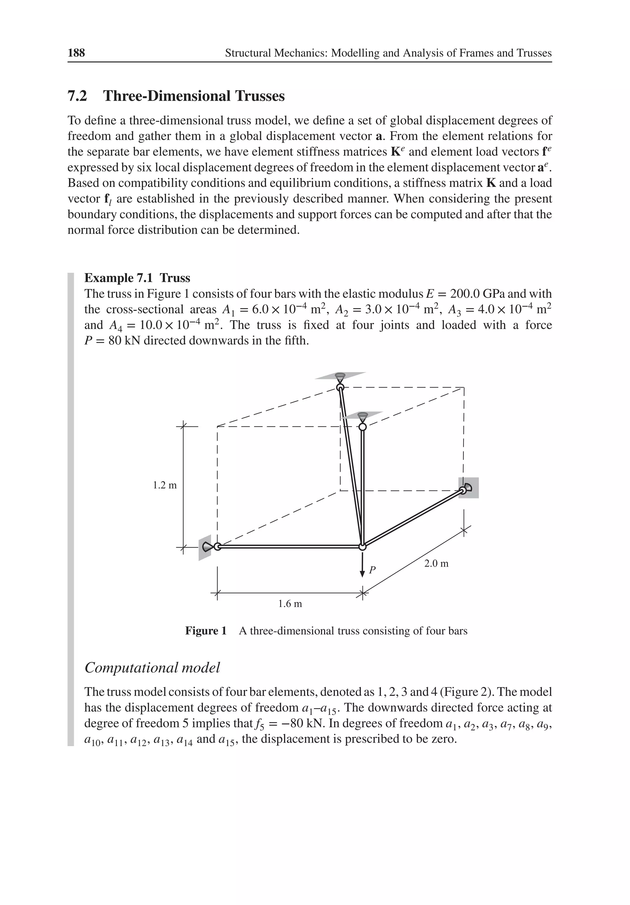
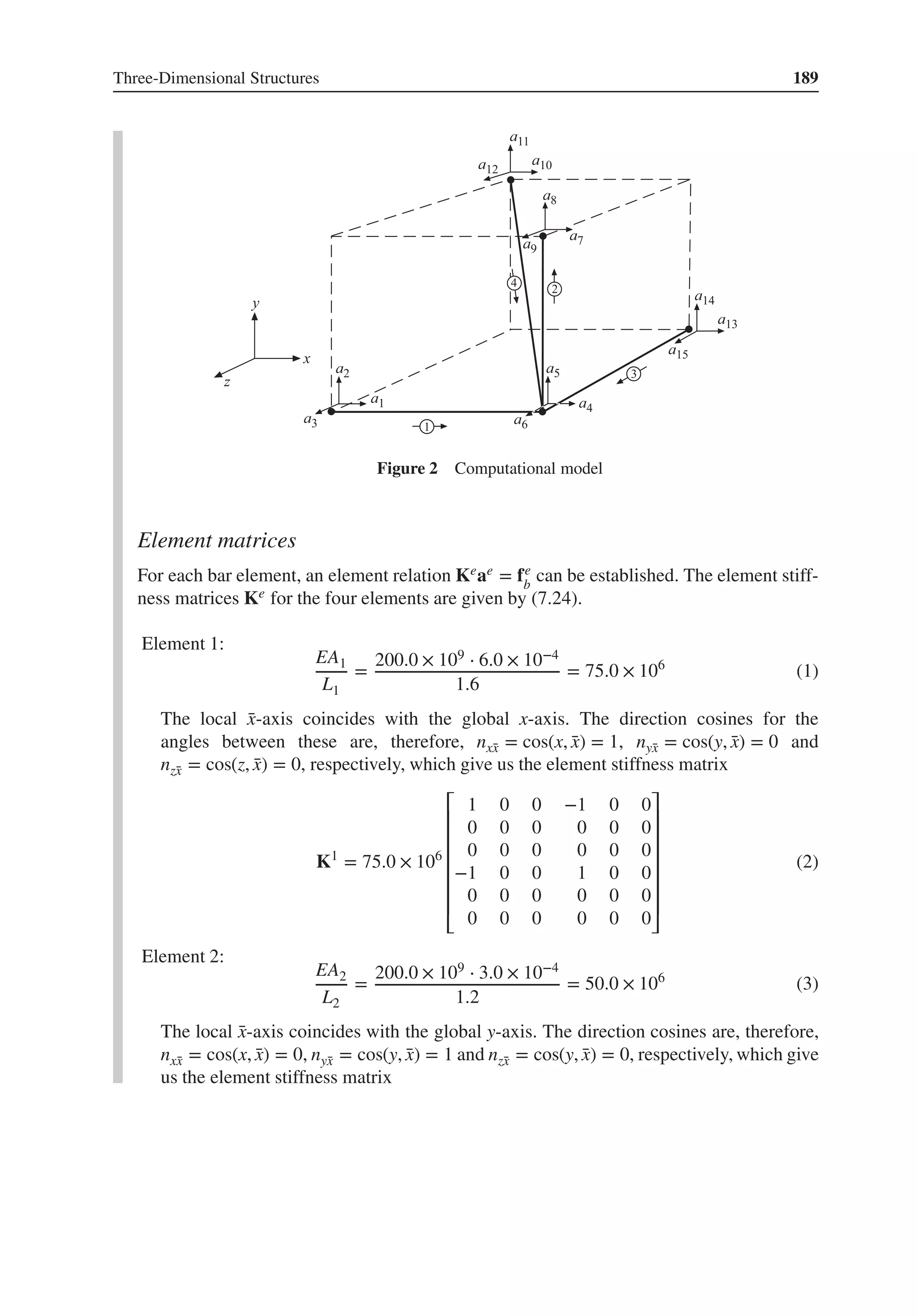
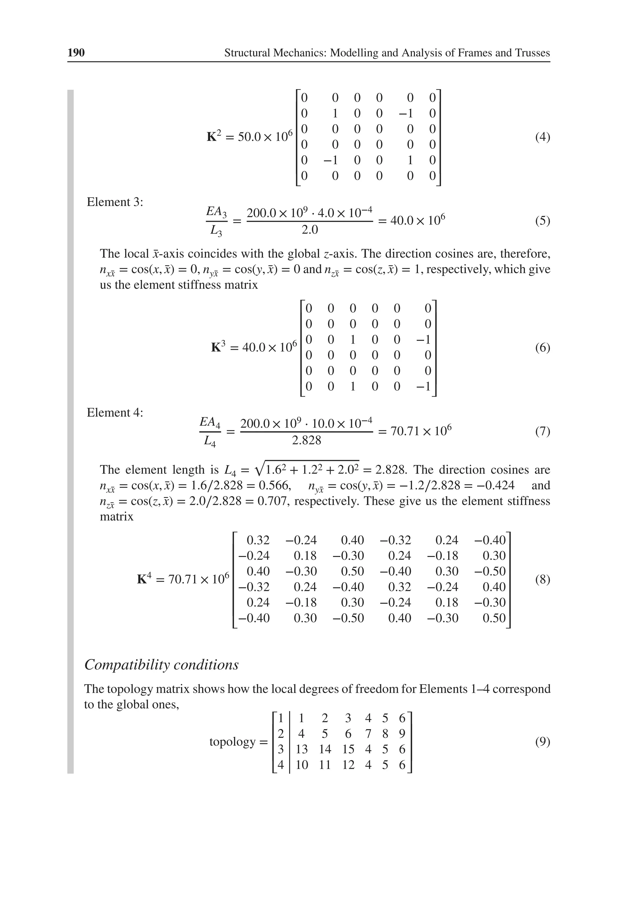
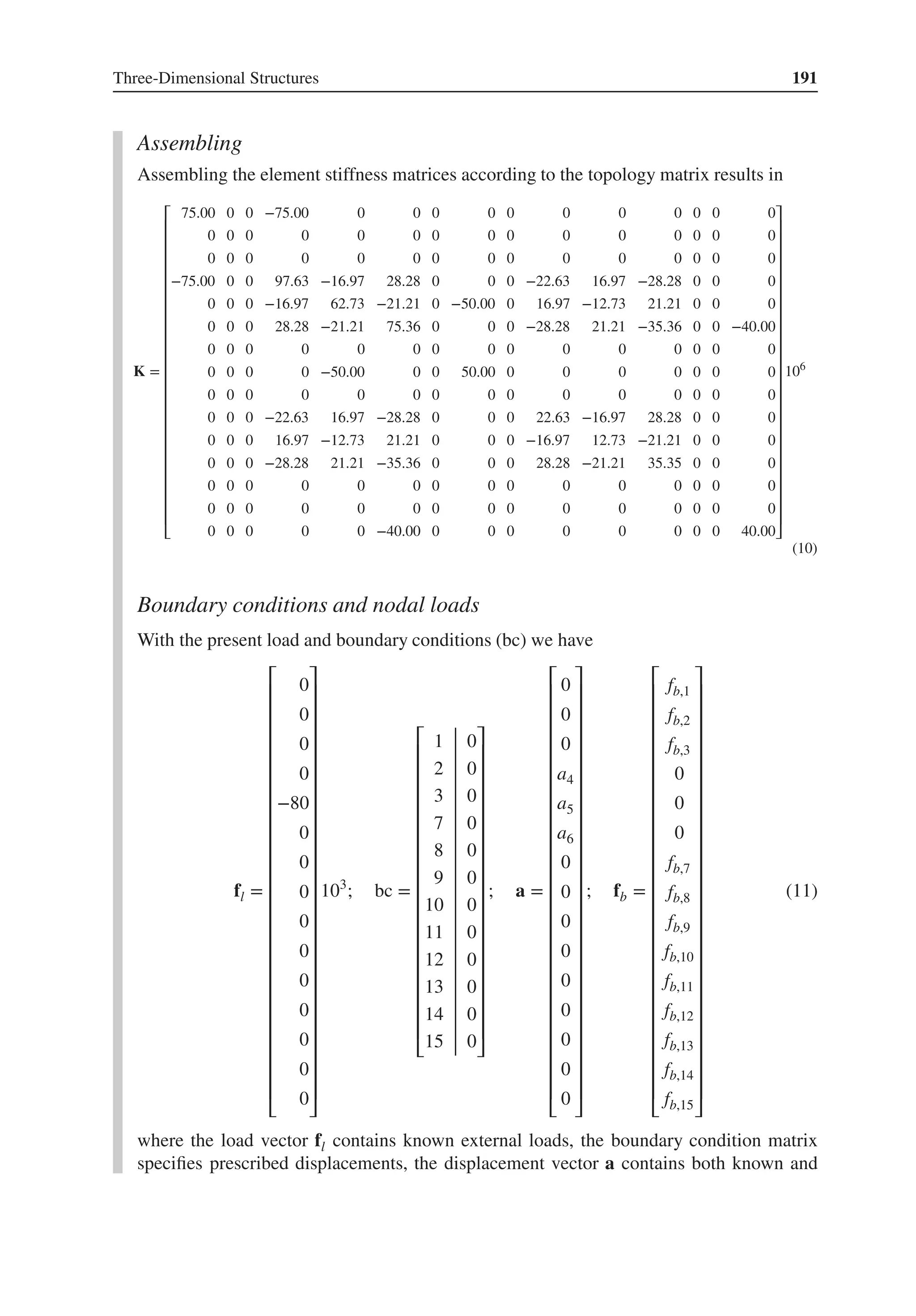
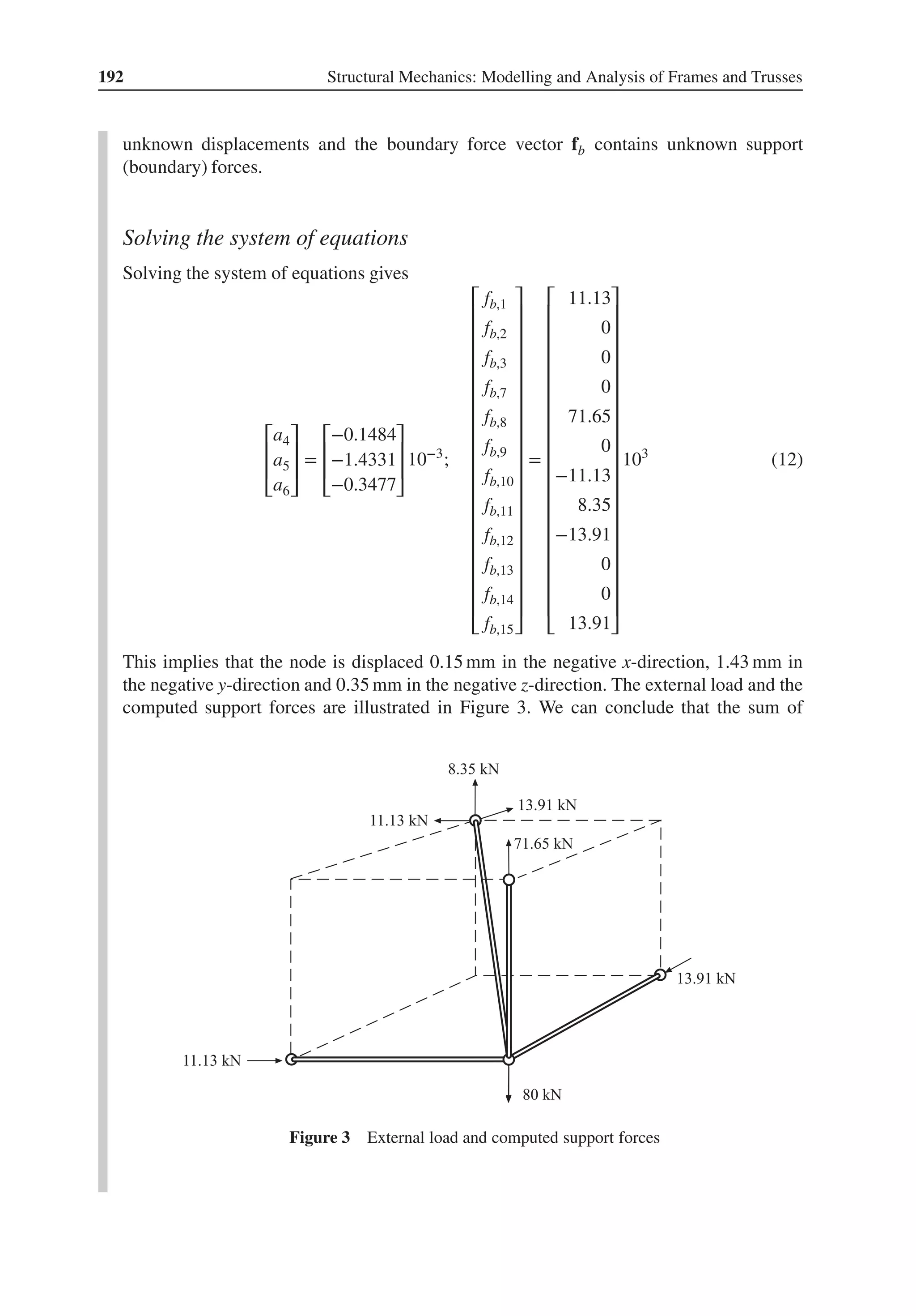
![Three-Dimensional Structures 193
the external forces in the x-, y- and z-direction, respectively, is equal to zero. Thus, the
equilibrium is satisfied.
Internal forces
Using (7.11), the displacements can be expressed in the local coordinate system of the
element. For Element 1, we obtain:
̄
a1
= Ga1
=
[
1 0 0 0 0 0
0 0 0 1 0 0
]
⎡
⎢
⎢
⎢
⎢
⎢
⎢
⎣
0
0
0
−0.1484
−1.4331
−0.3477
⎤
⎥
⎥
⎥
⎥
⎥
⎥
⎦
10−3
=
[
0
−0.1484
]
10−3
(13)
With the local displacements known, the normal force in Element 1 can be computed using
(3.52)
N(1)
= EA1B̄
a1
= 200.0 × 109
× 6.0 × 10−4 1
1.6
[
−1 1
]
[
0
−0.1484
]
10−3
= −11.13 × 10³
(14)
For Elements 2–4 we have, with the corresponding computations
N(2)
= 71.65 × 10³
(15)
N(3)
= −13.91 × 10³
(16)
N(4)
= 19.67 × 10³
(17)
These results imply that the normal forces in the four elements are −11.13, 71.65, −13.91
and 19.67 kN, respectively; see Figure 4.
Figure 4 Normal forces in the bars](https://image.slidesharecdn.com/structuralmechanicsmodellingandanalysisofframesandtrussespdfdrive-230720064114-5e1f9a93/75/Structural-mechanics-_-modelling-and-analysis-of-frames-and-trusses-PDFDrive-pdf-207-2048.jpg)
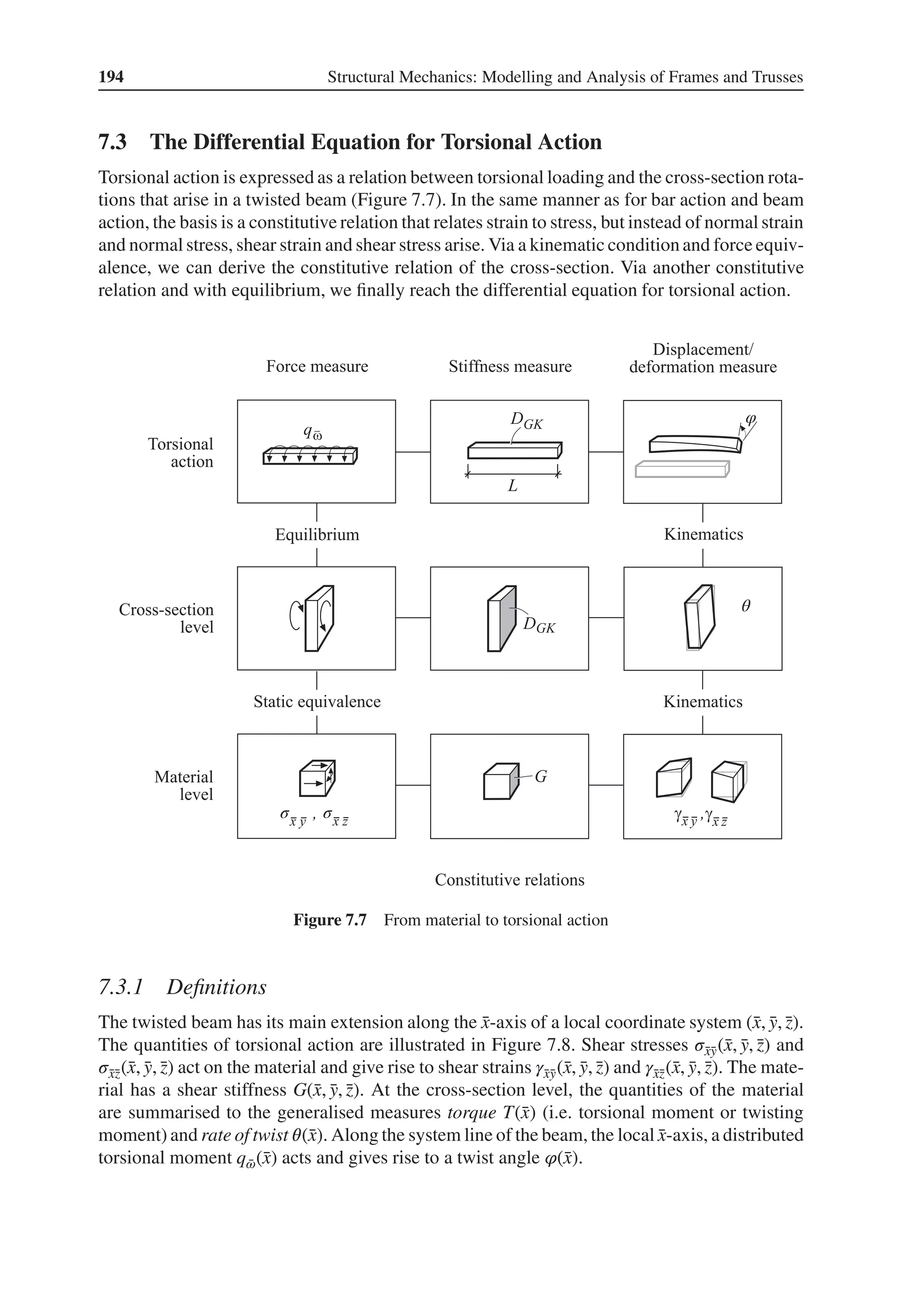
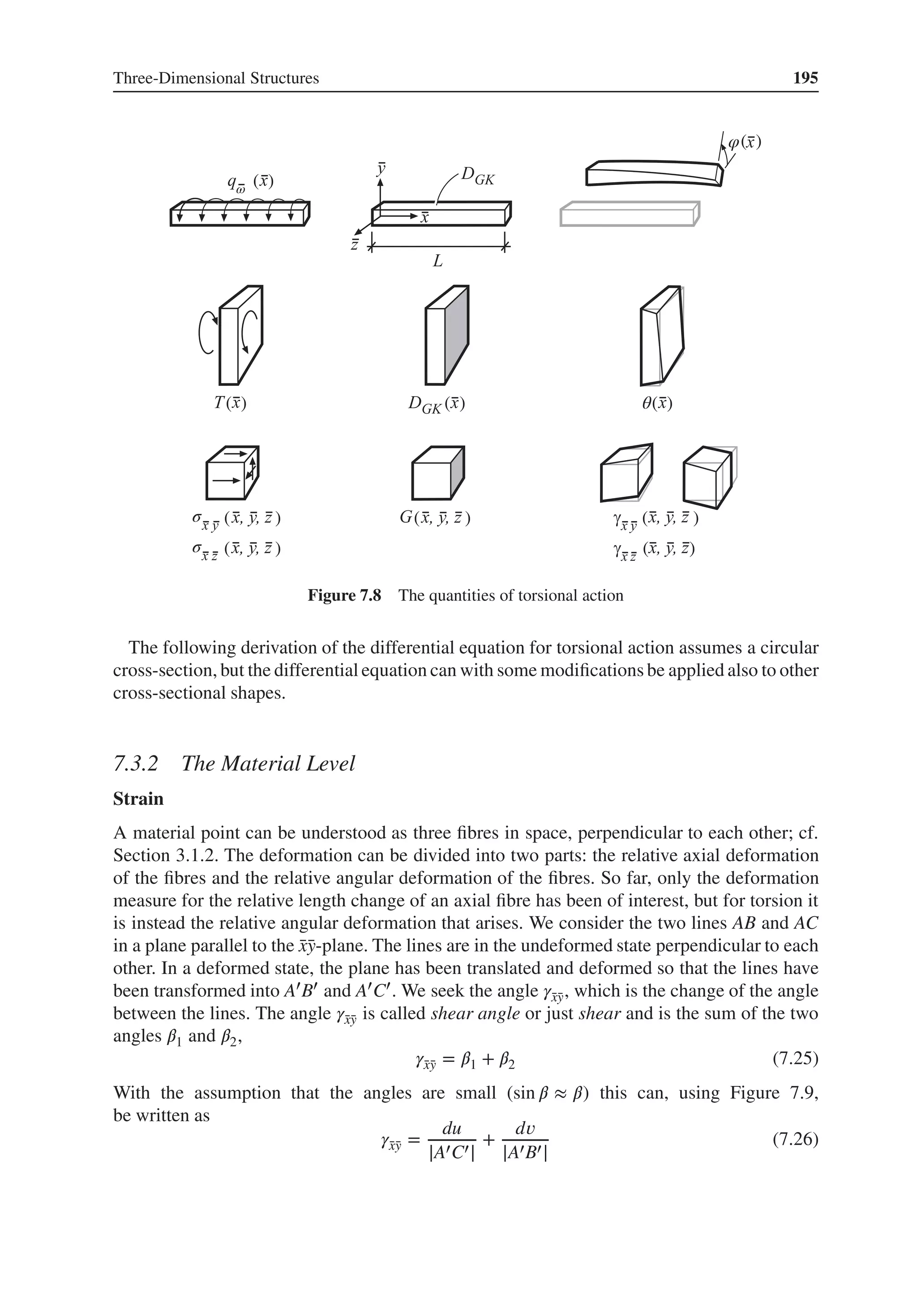
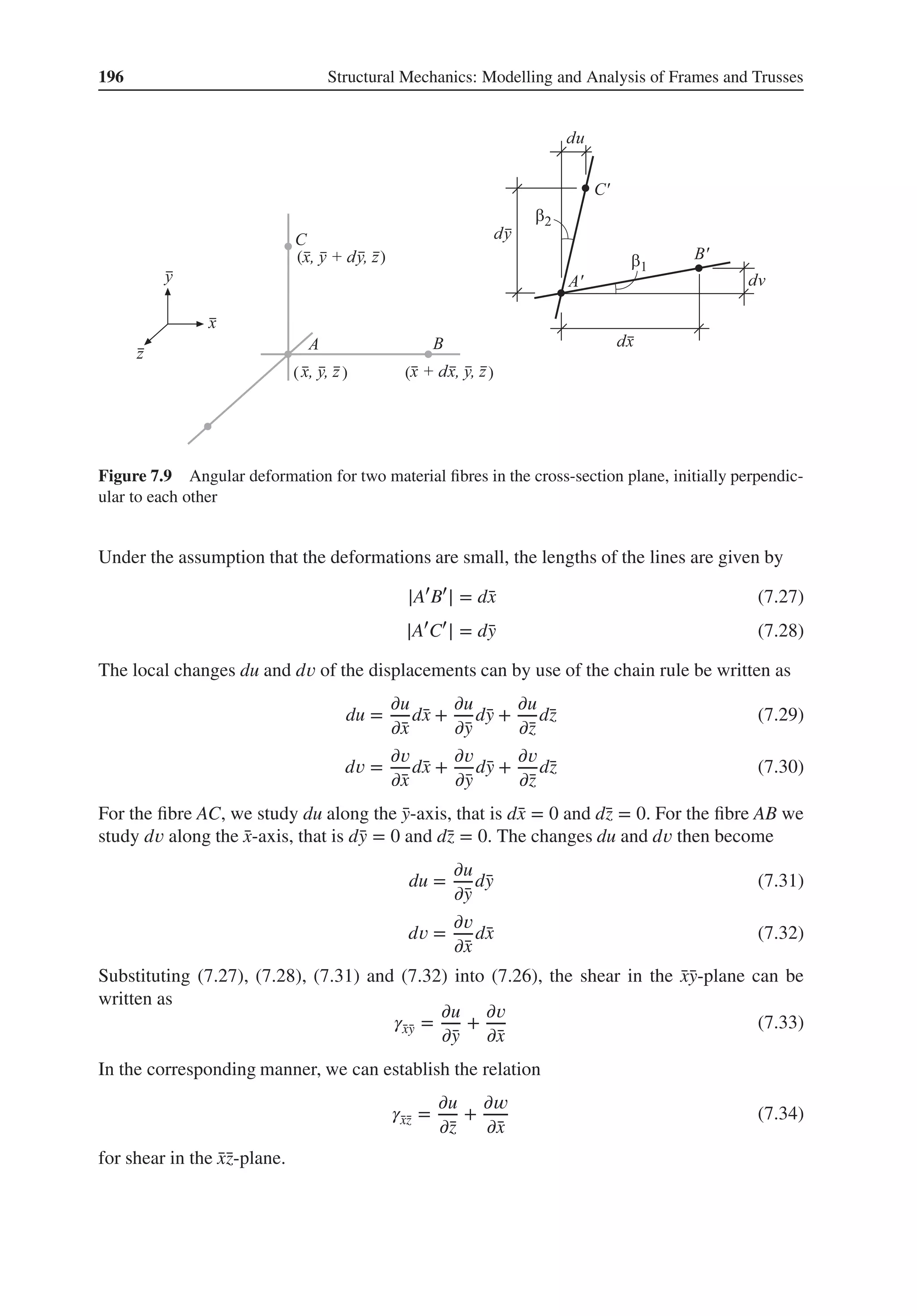
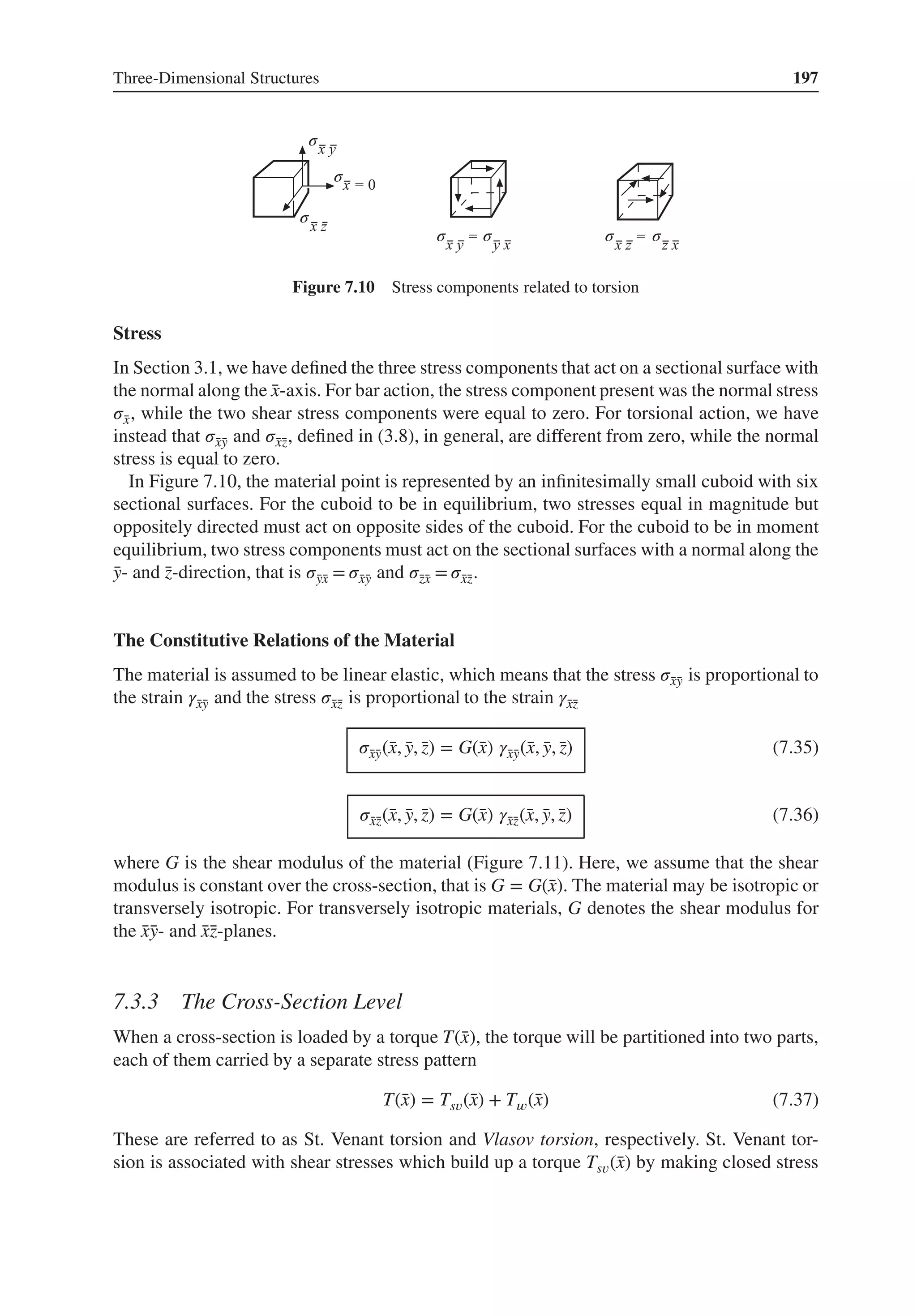
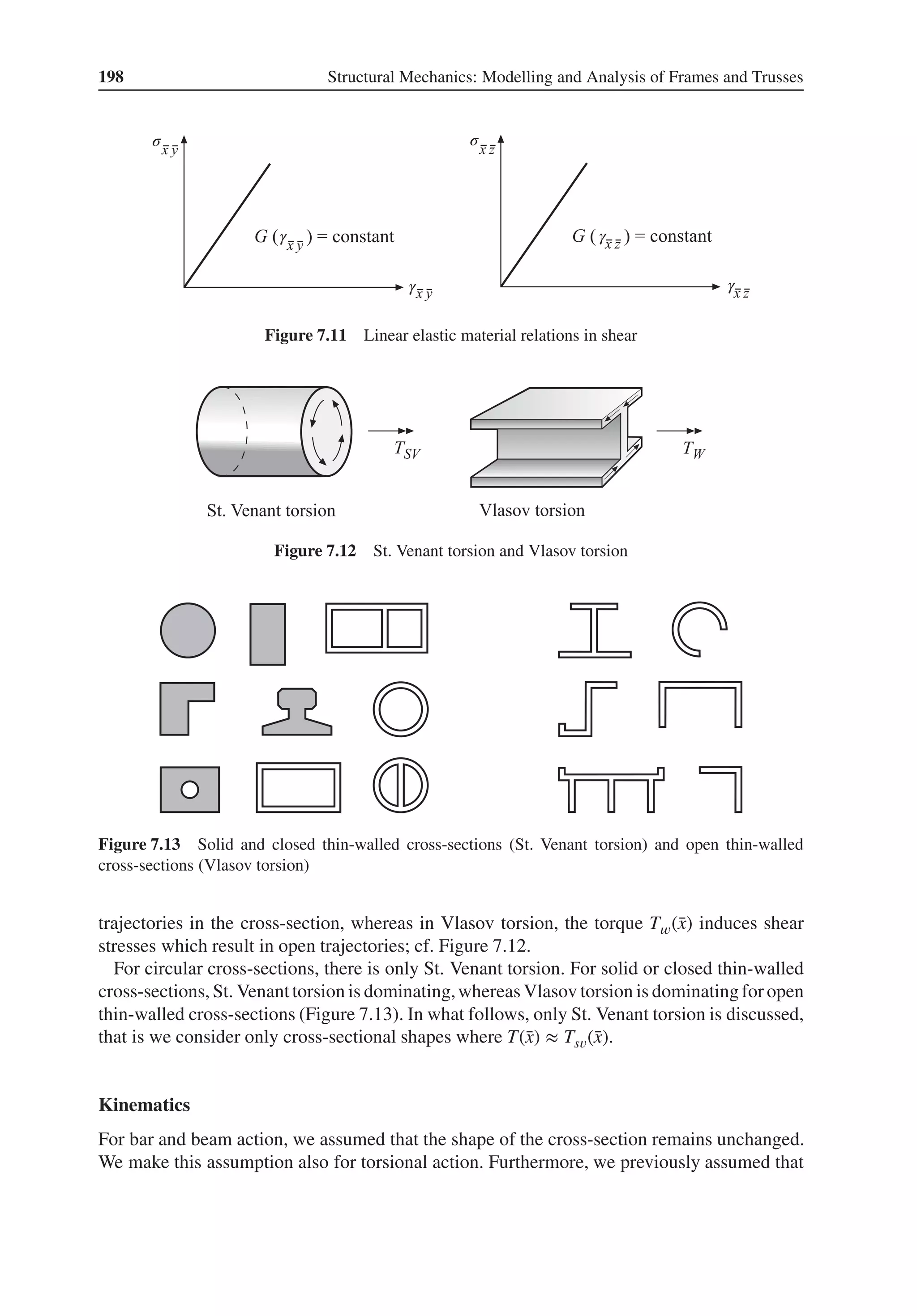
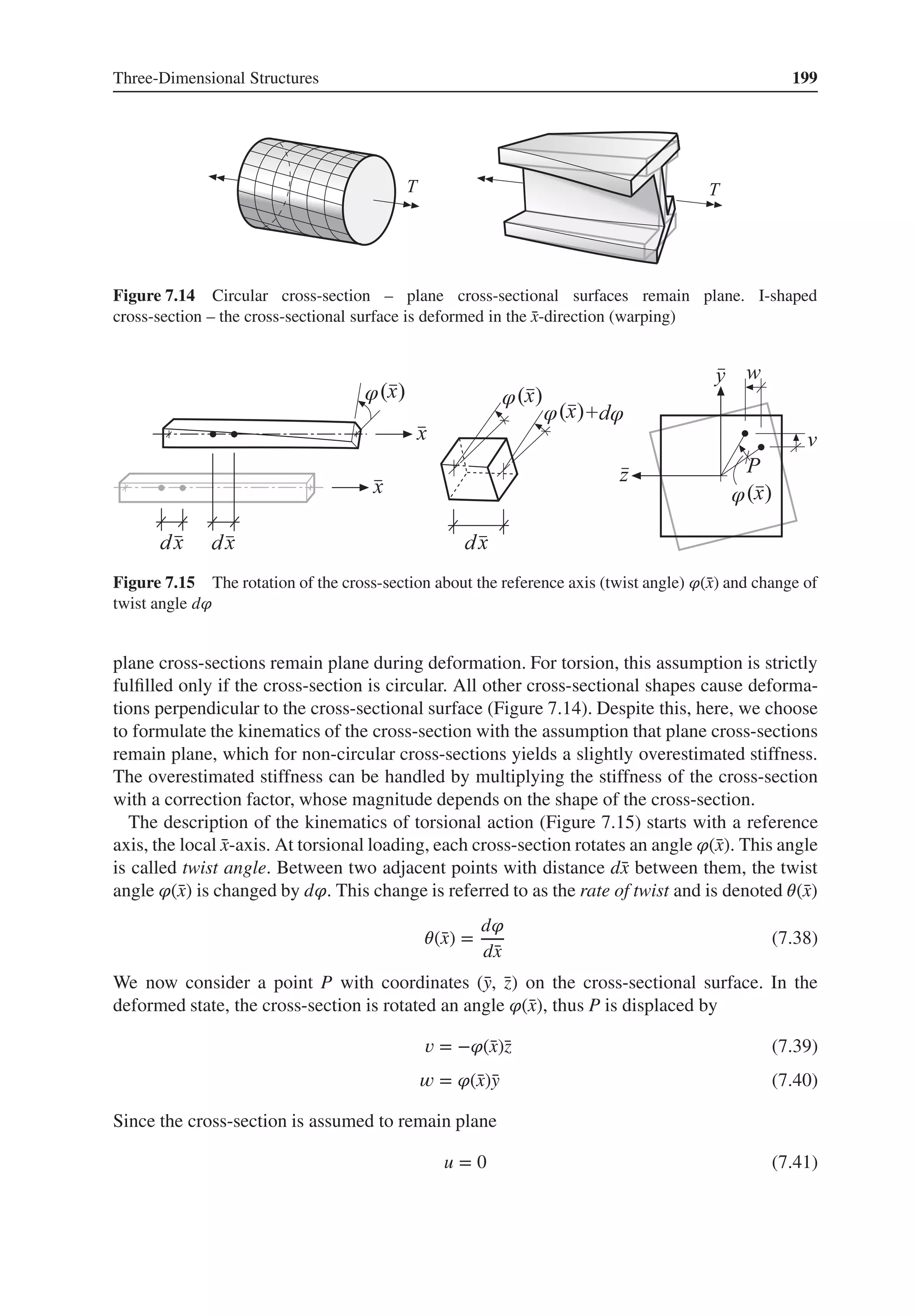
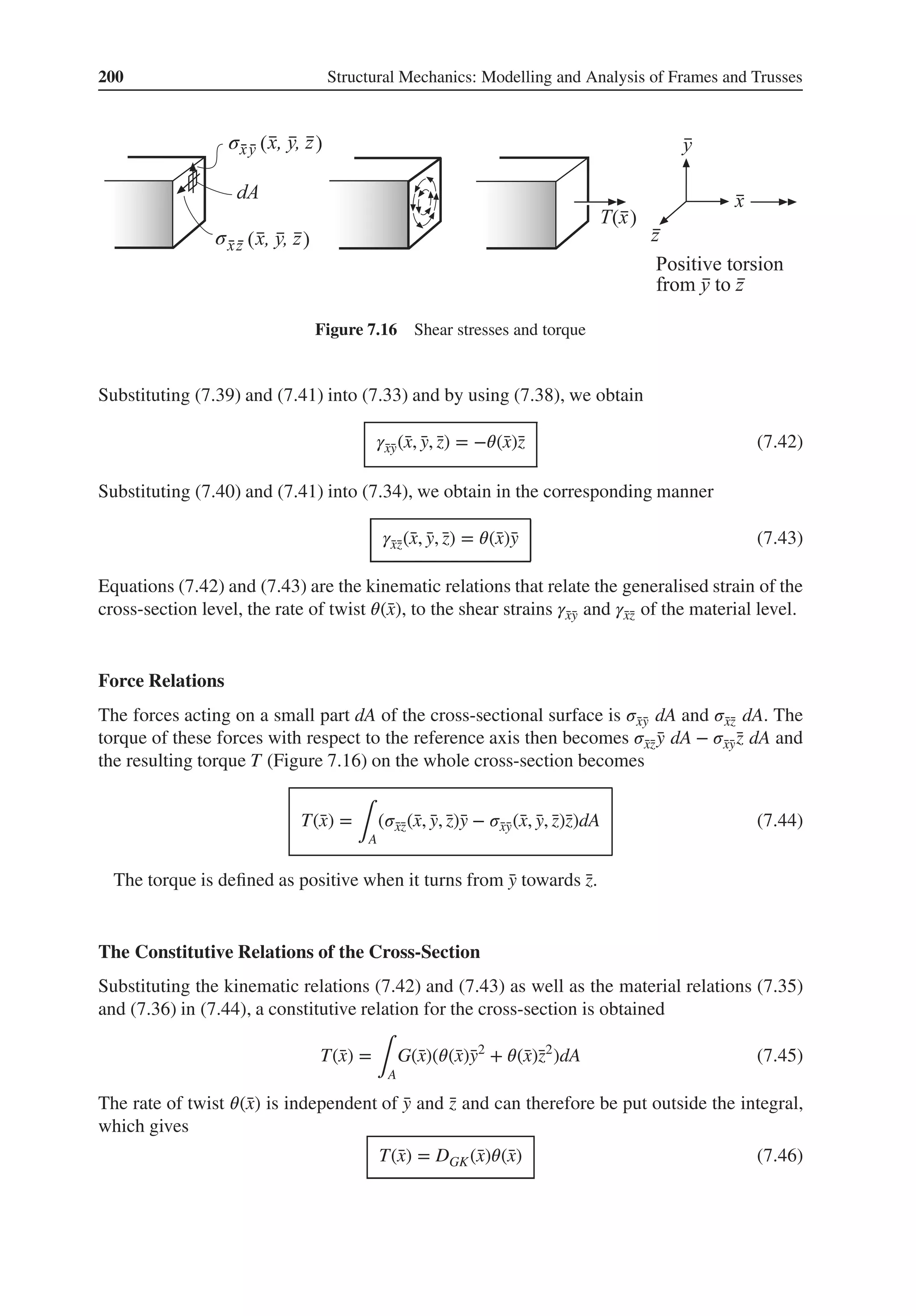
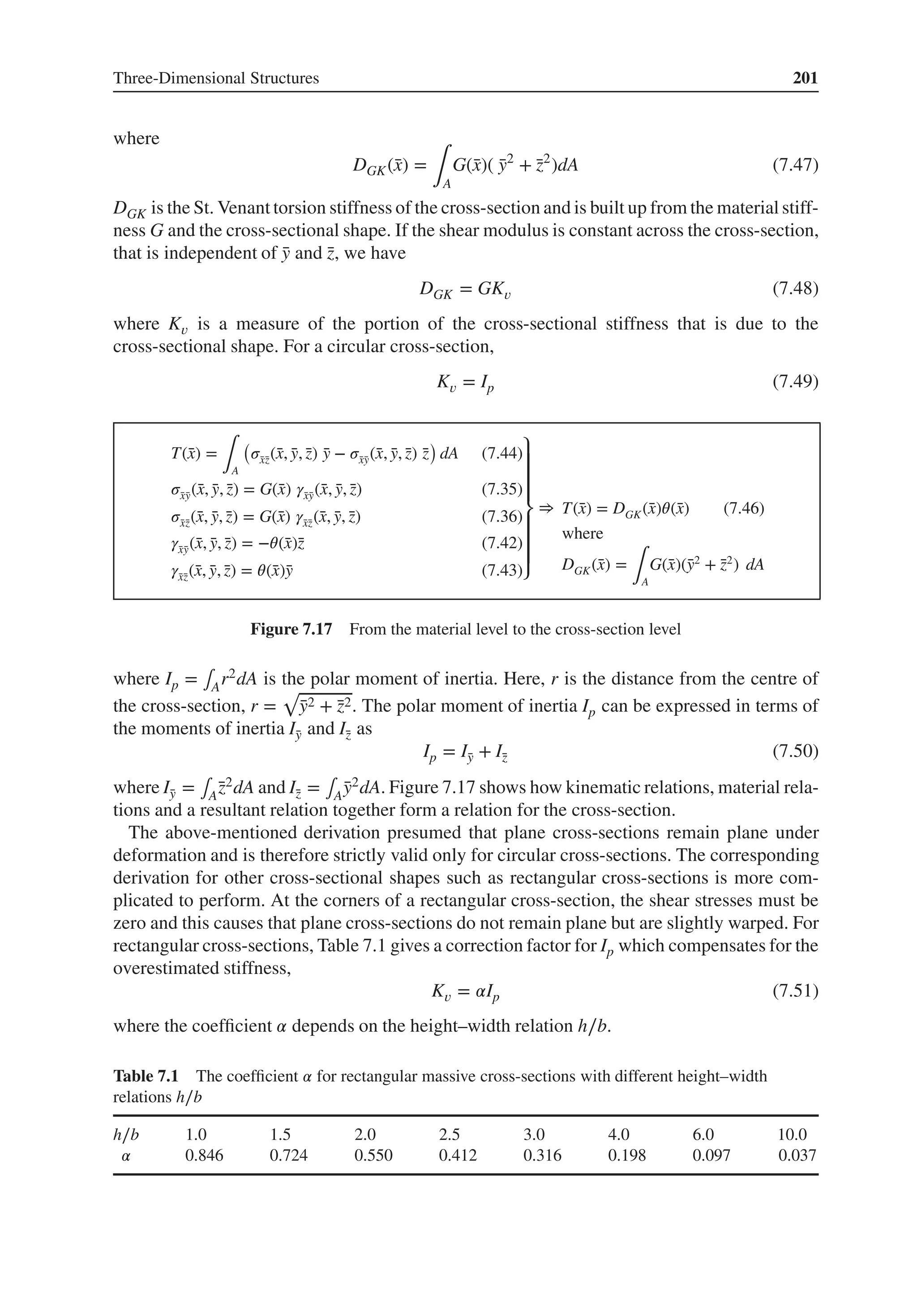
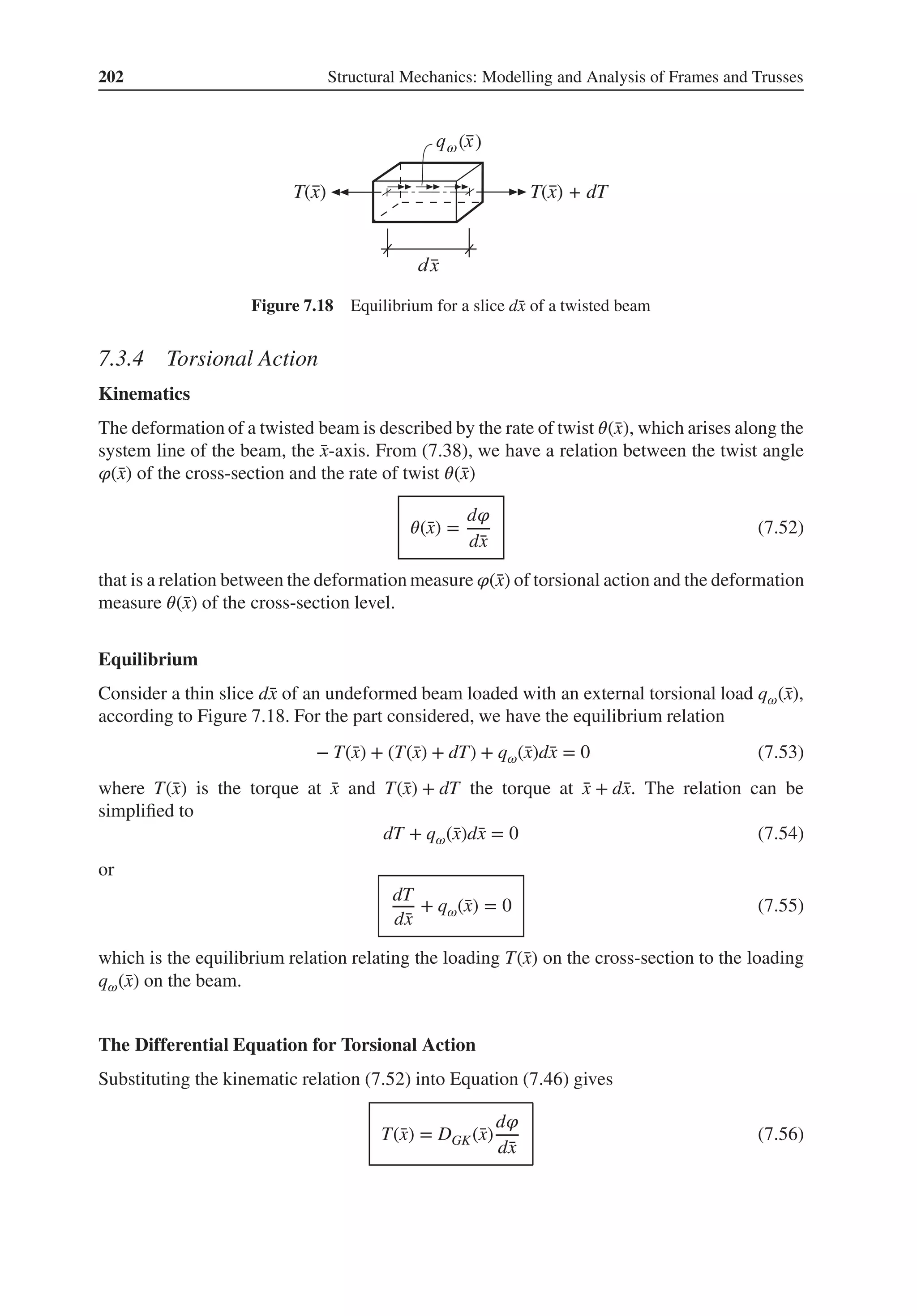
![204 Structural Mechanics: Modelling and Analysis of Frames and Trusses
Figure 7.20 Three-dimensional beam element
Figure 7.21 Element for pure torsional action
7.4.1 Element for Torsional Action
We start by formulating an element for pure torsional action. Such an element has two dis-
placement degrees of freedom, ̄
u1 and ̄
u2 (Figure 7.21). The degrees of freedom describe the
rotation about the ̄
x-axis for ̄
x = 0 and for ̄
x = L. The torques acting at ̄
x = 0 and ̄
x = L are
denoted ̄
P1 and ̄
P2, respectively, and are positive when directed as the rotations ̄
u1 and ̄
u2.
The differential equation for torsional action (7.52) is built in the same manner as the dif-
ferential equation for bar action (3.25), but with different variables and constants. Thus, the
solution is obtained in the same manner. Therefore, we can by using the solution for bar action
establish the solution for torsional action in matrix form as
̄
Ke
̄
ae
= ̄
fe
(7.60)
where
̄
Ke
=
DGK
L
[
1 −1
−1 1
]
(7.61)
̄
ae
=
[
̄
u1
̄
u2
]
(7.62)
̄
fe
= ̄
fe
b + ̄
fe
l (7.63)
̄
fe
b =
[
̄
P1
̄
P2
]
=
[
−T(0)
T(L)
]
(7.64)
̄
fe
l =
[
Tp(0)
−Tp(L)
]
(7.65)](https://image.slidesharecdn.com/structuralmechanicsmodellingandanalysisofframesandtrussespdfdrive-230720064114-5e1f9a93/75/Structural-mechanics-_-modelling-and-analysis-of-frames-and-trusses-PDFDrive-pdf-218-2048.jpg)
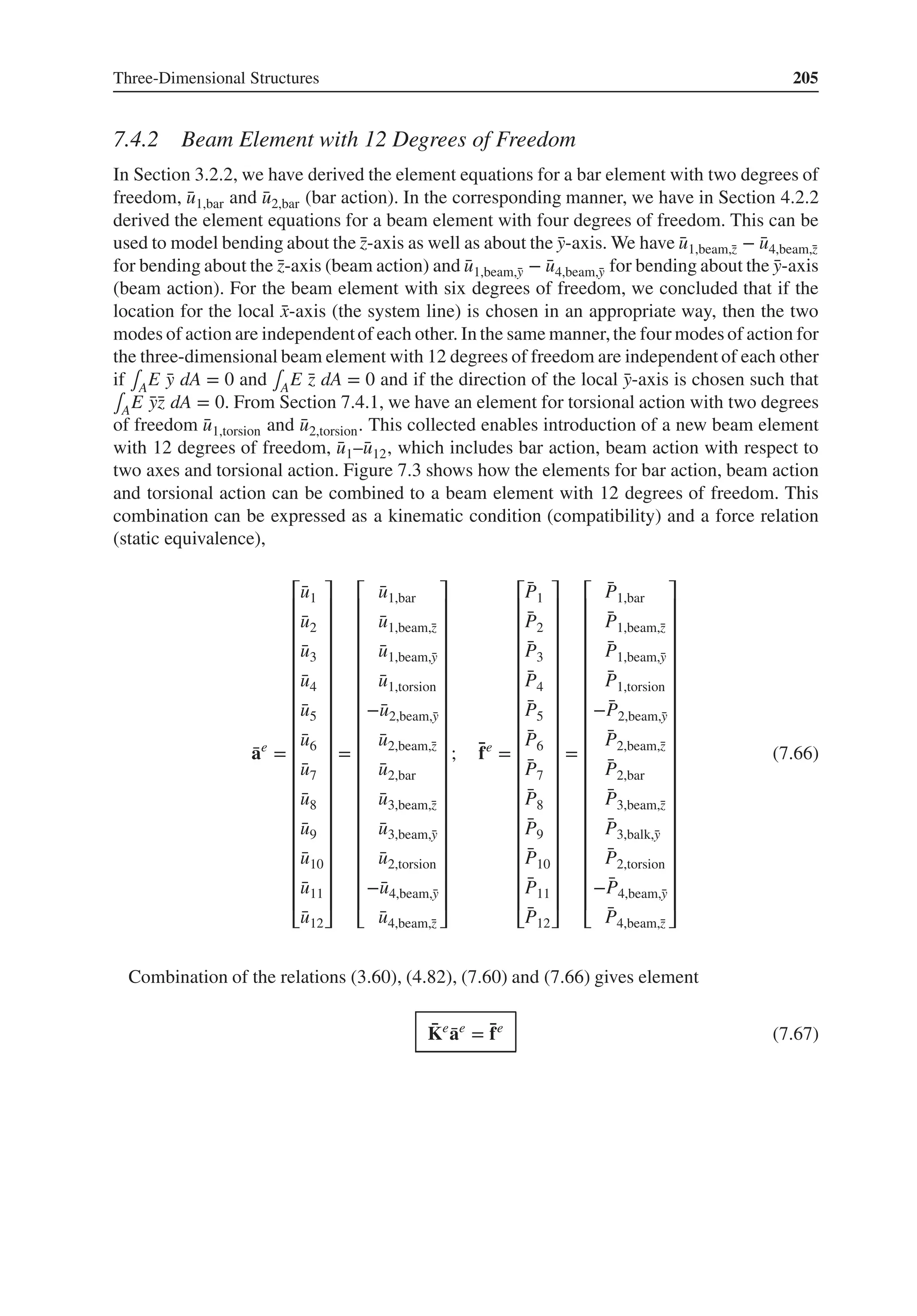
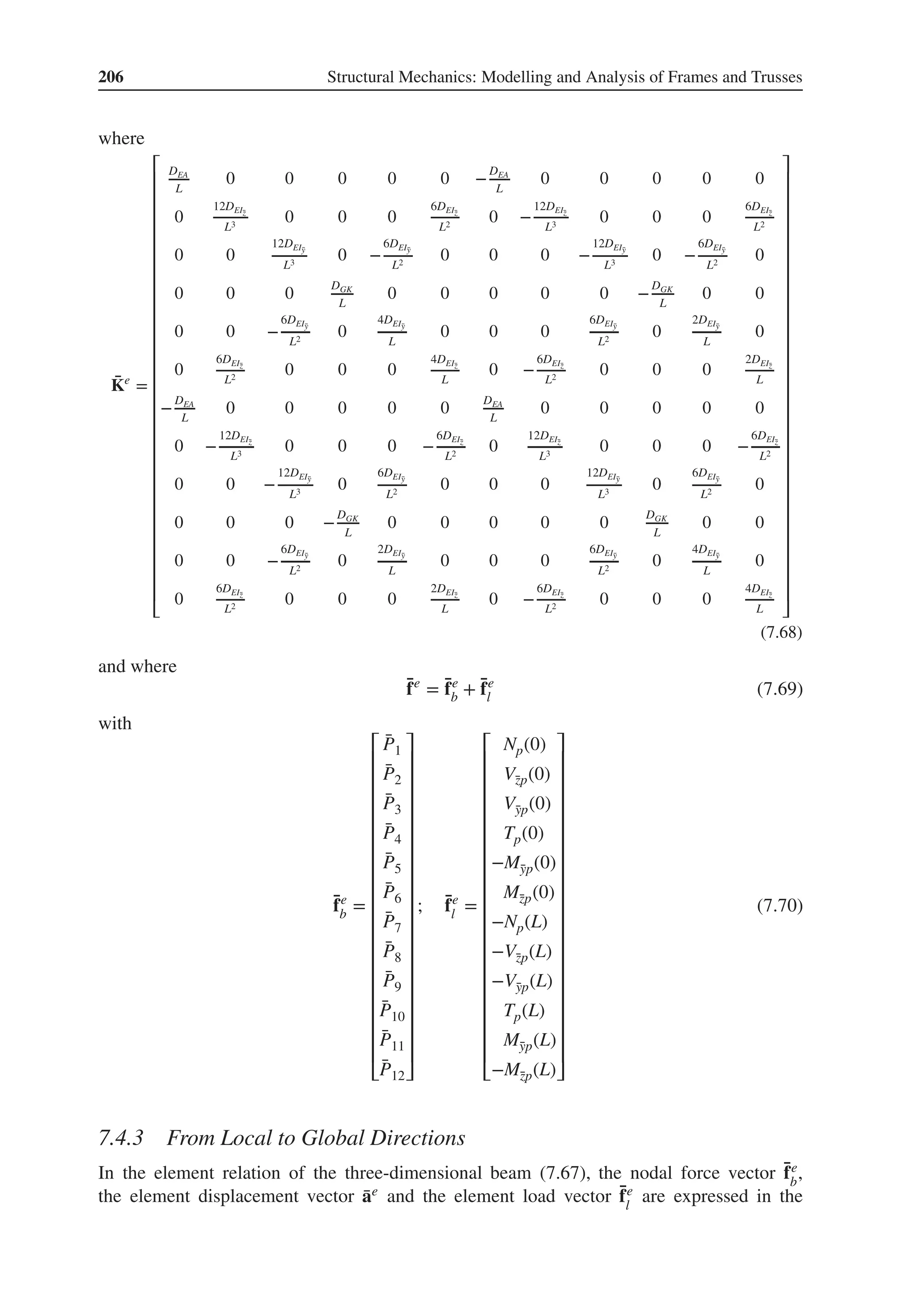
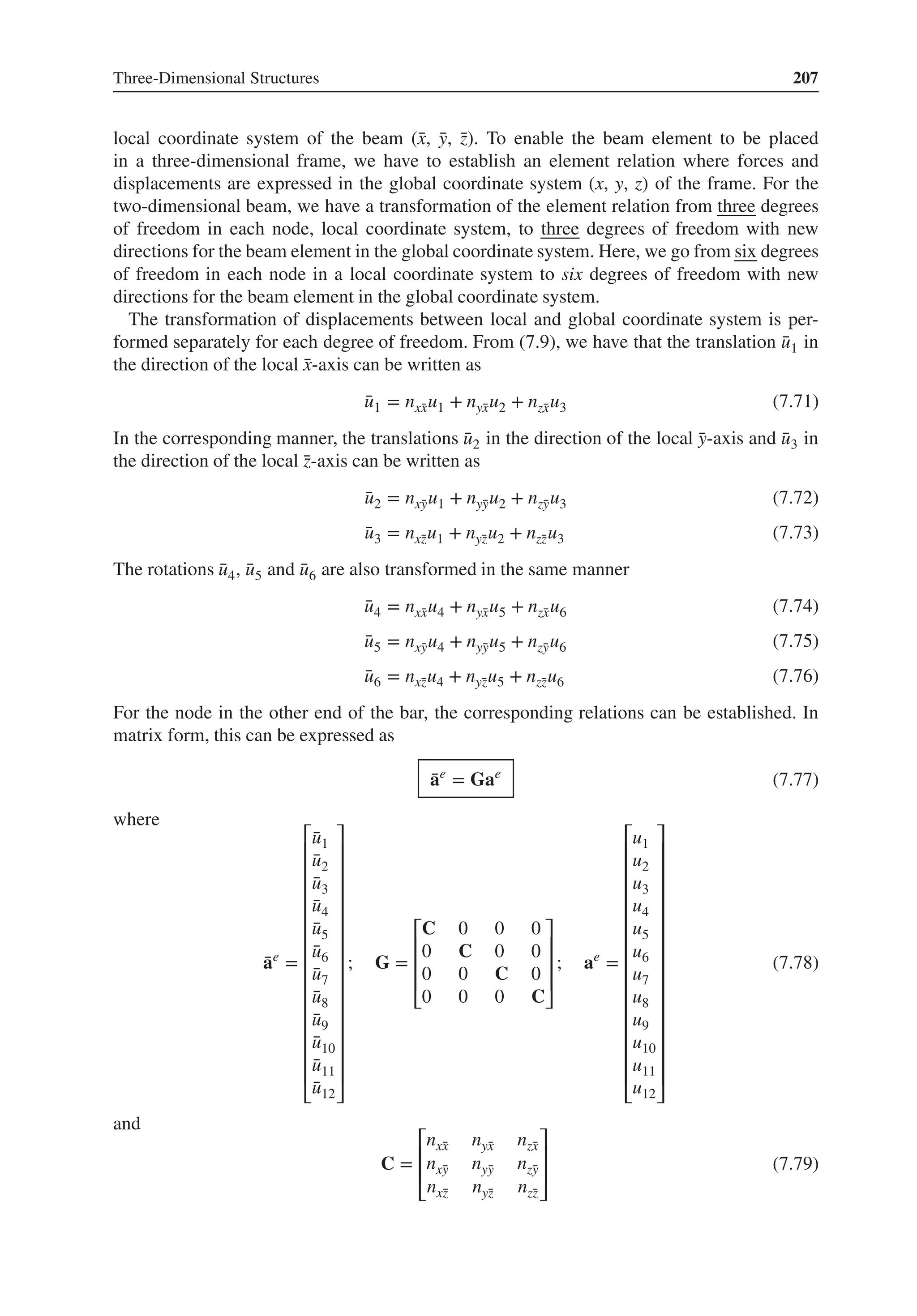
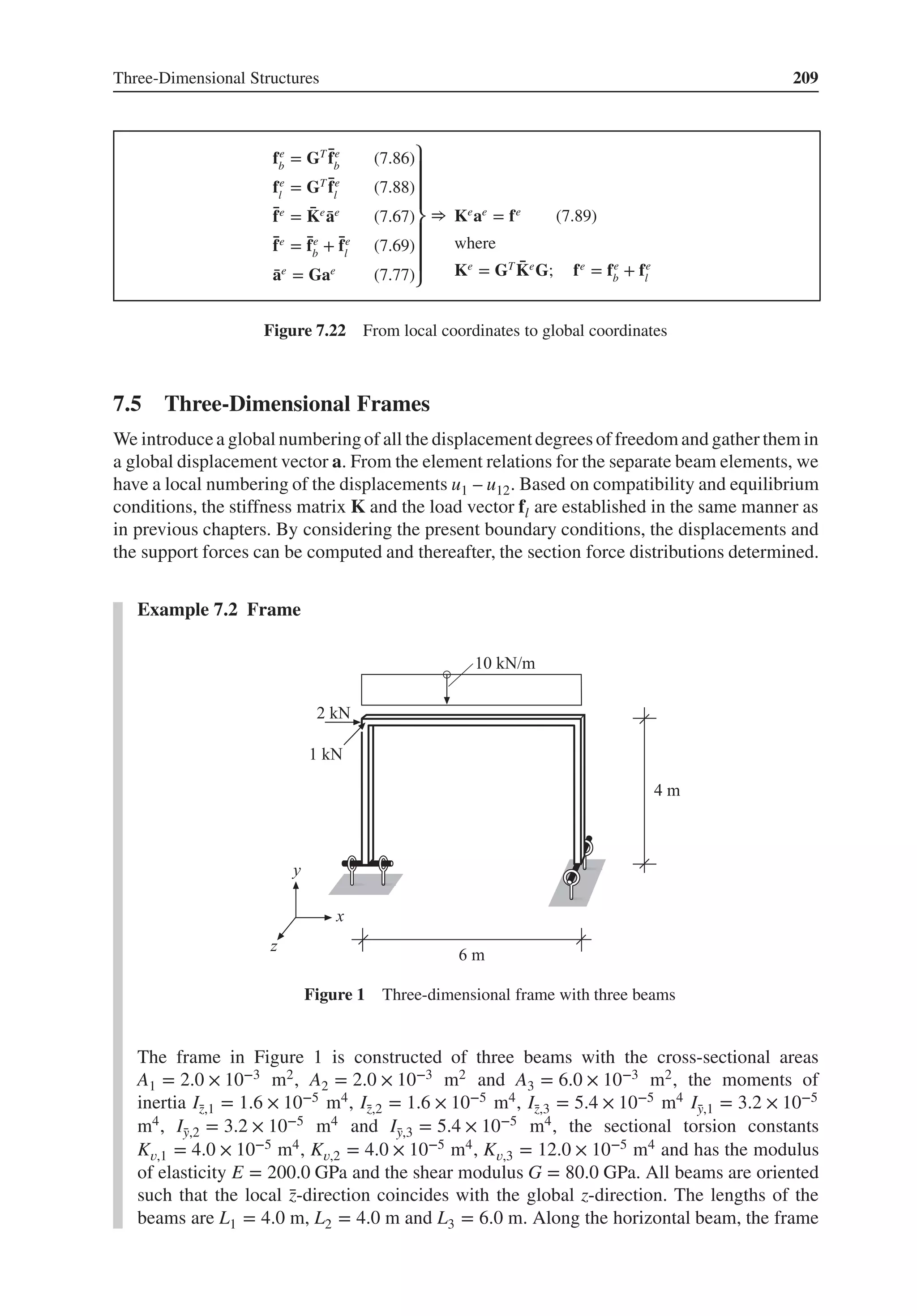
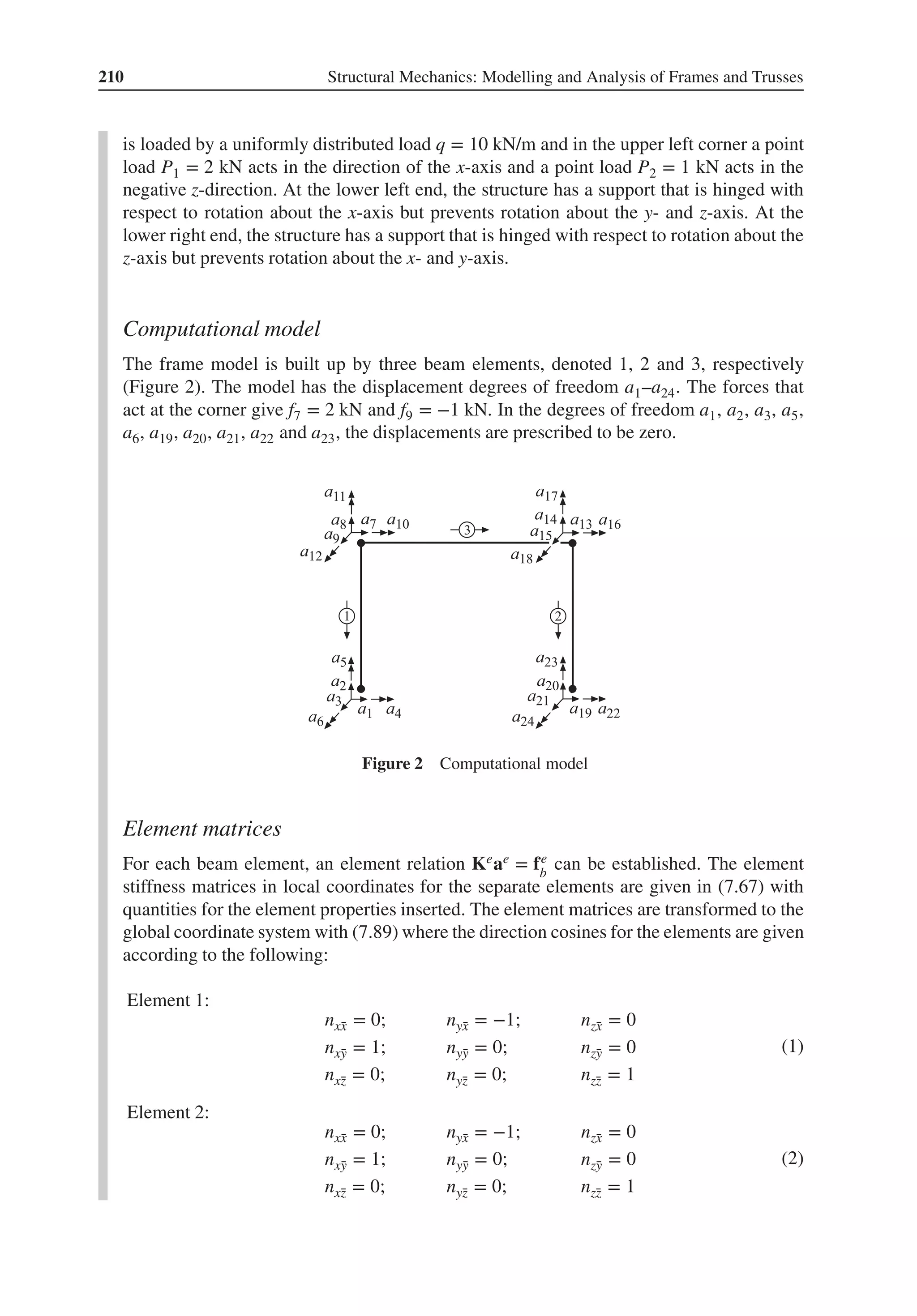
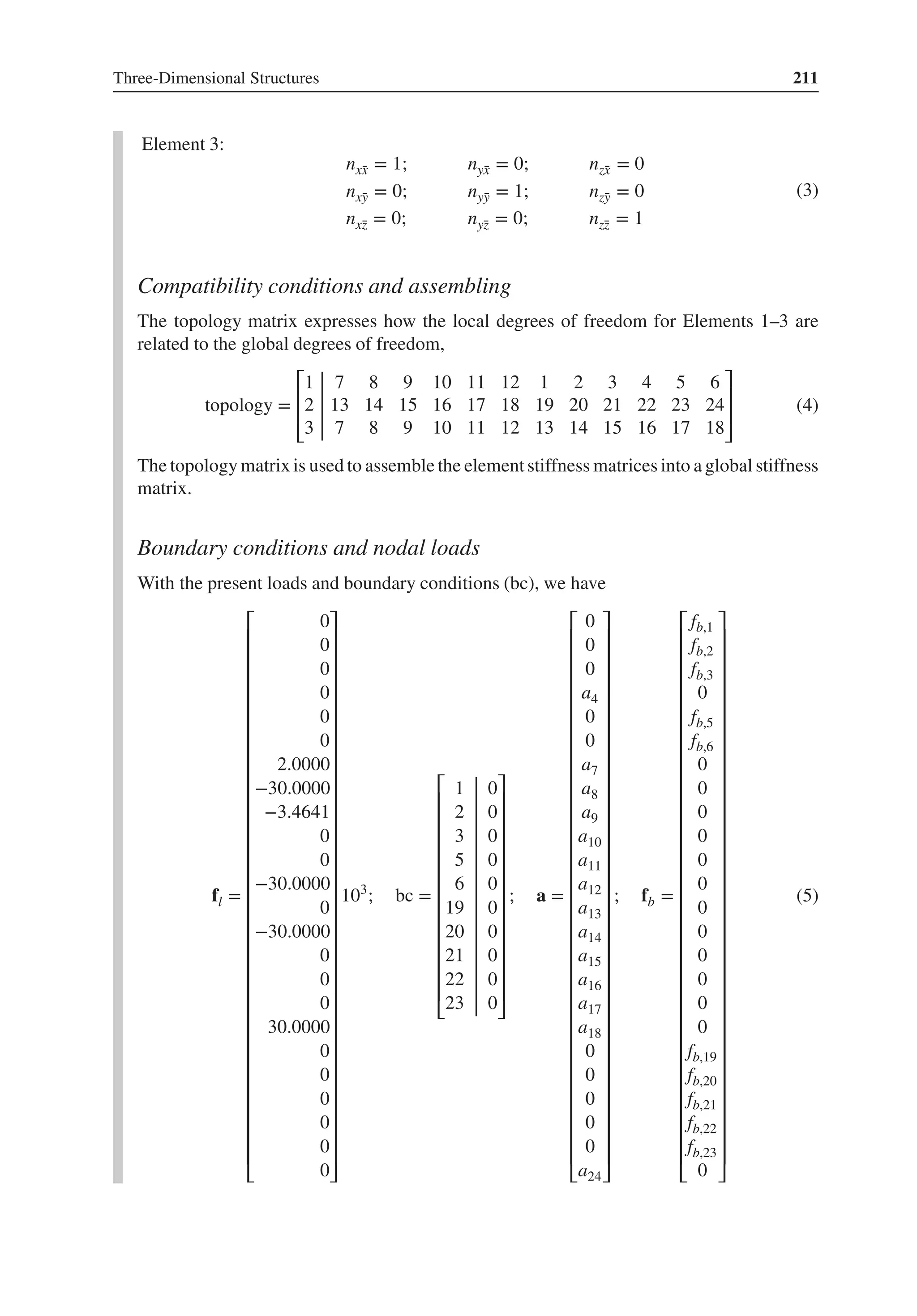
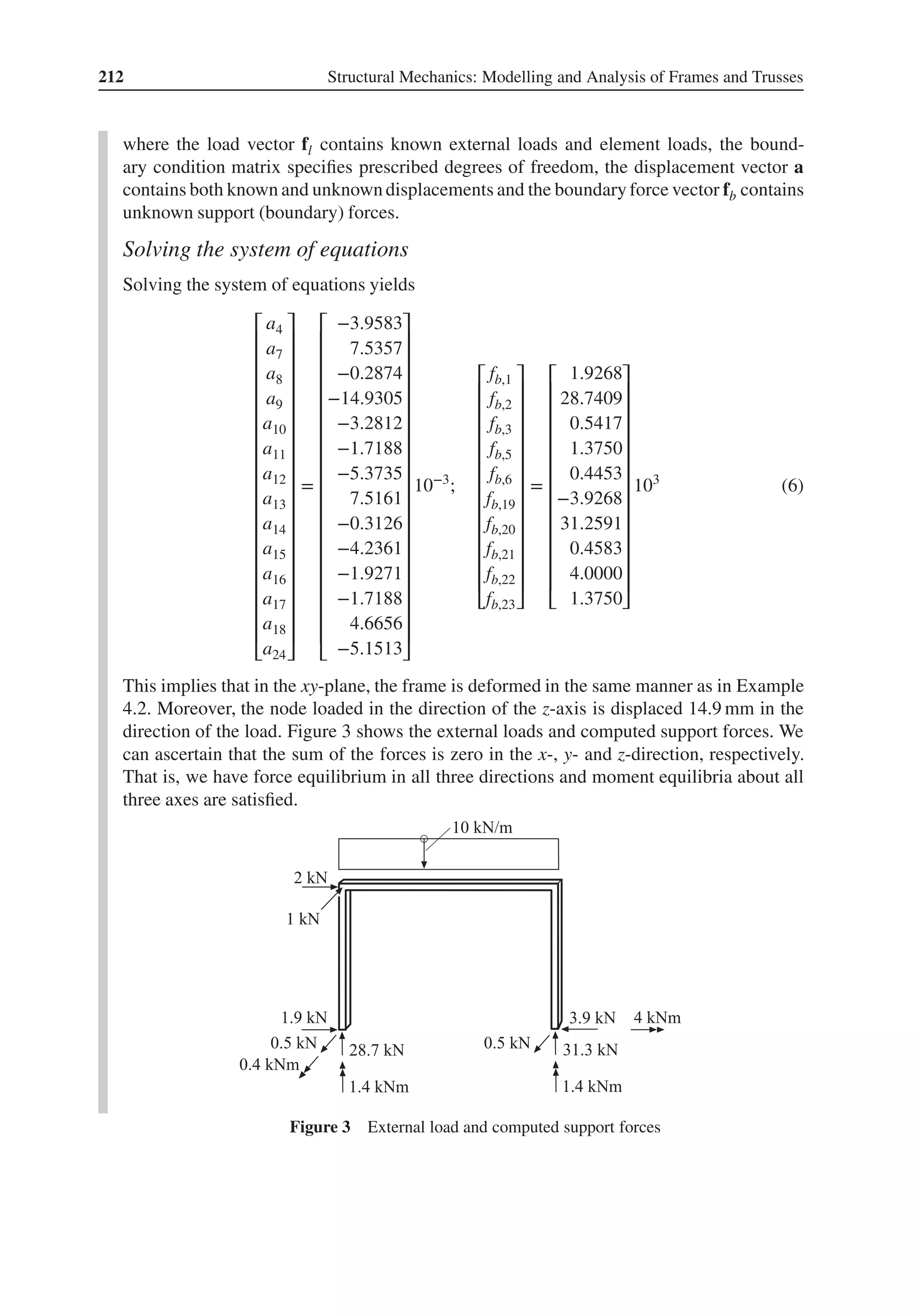
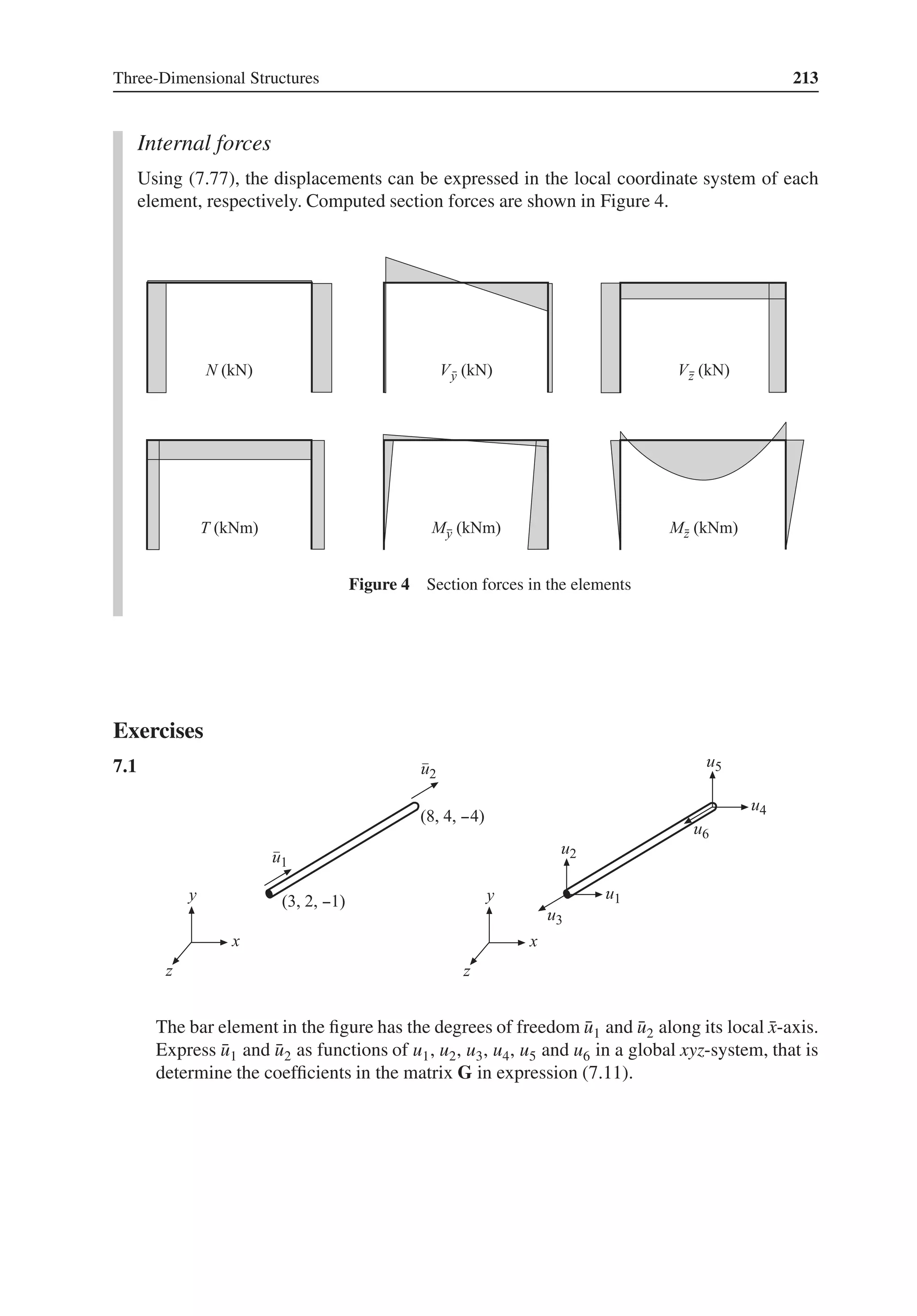
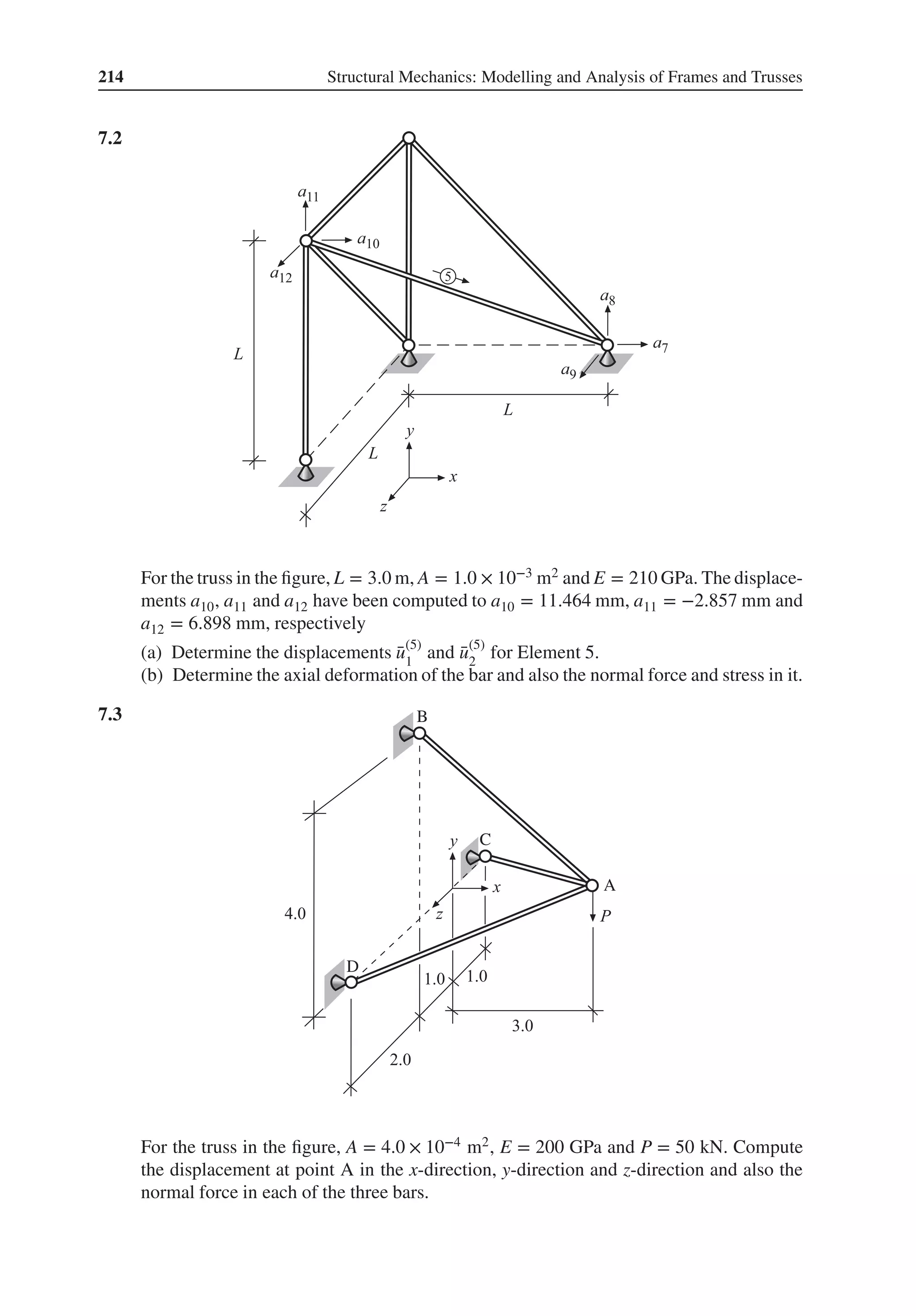
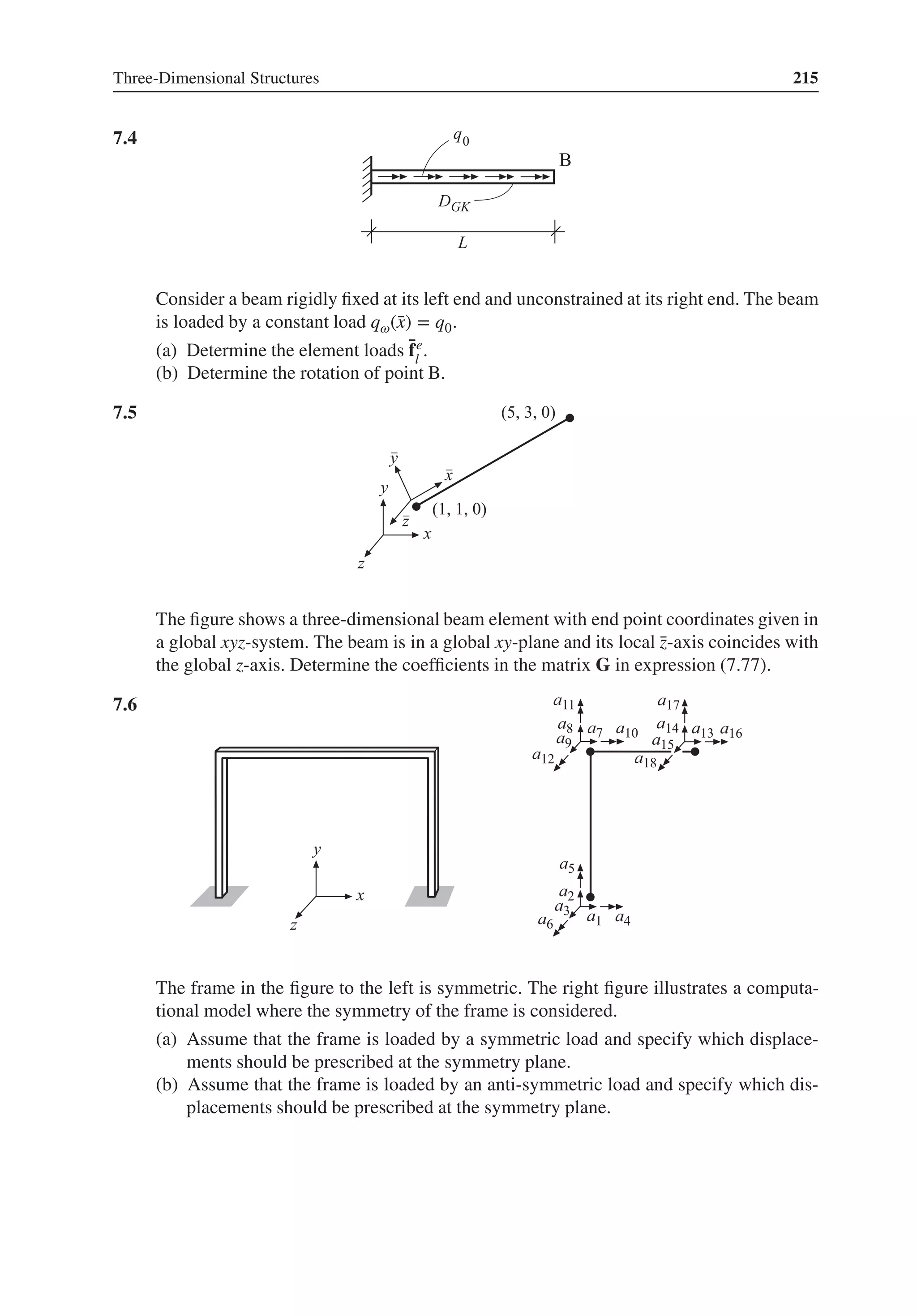
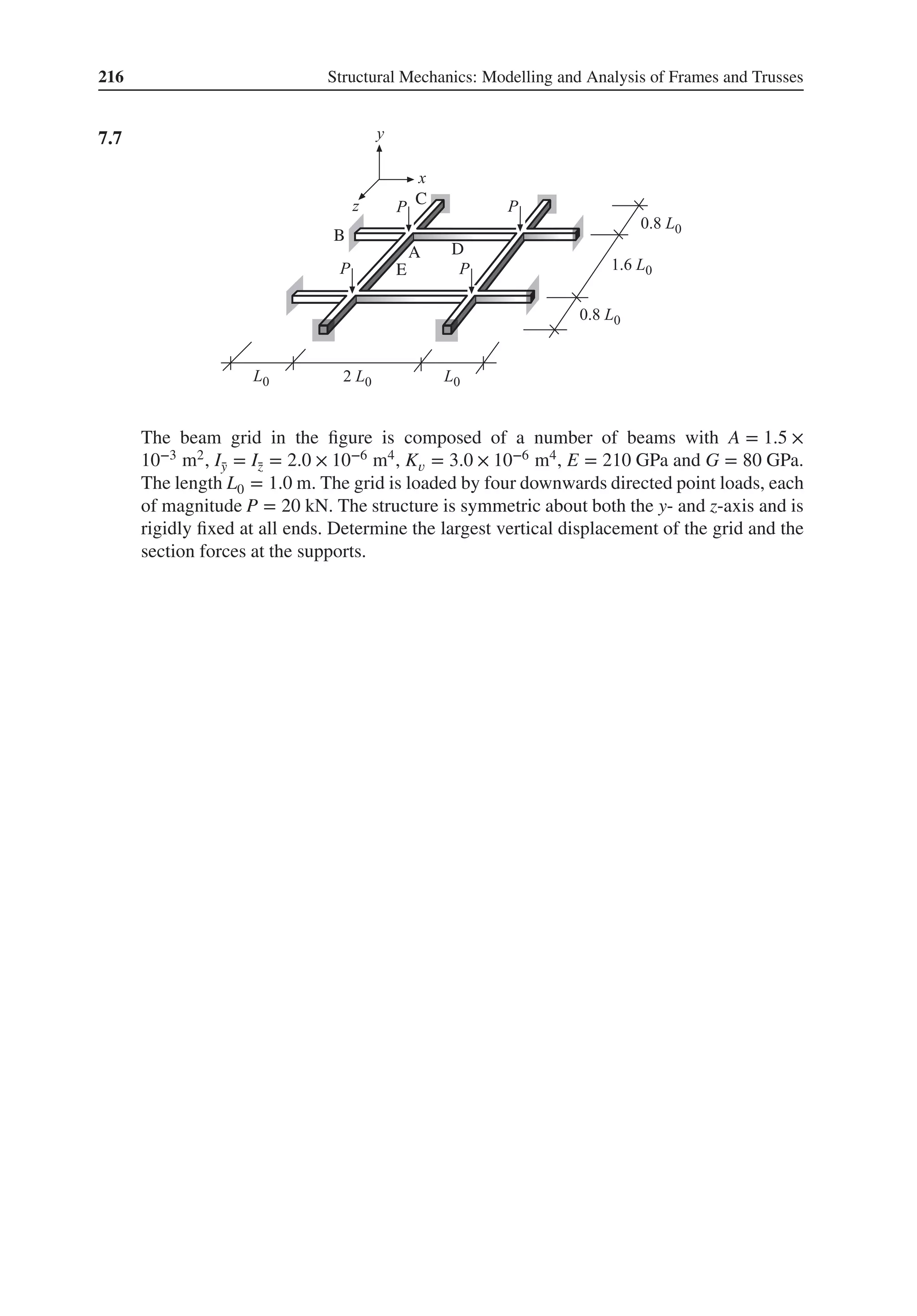
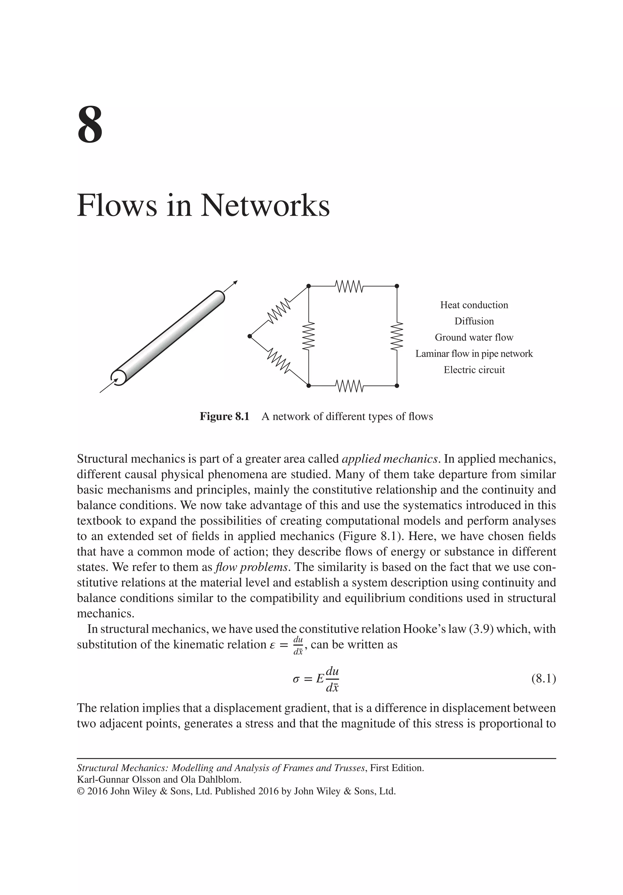
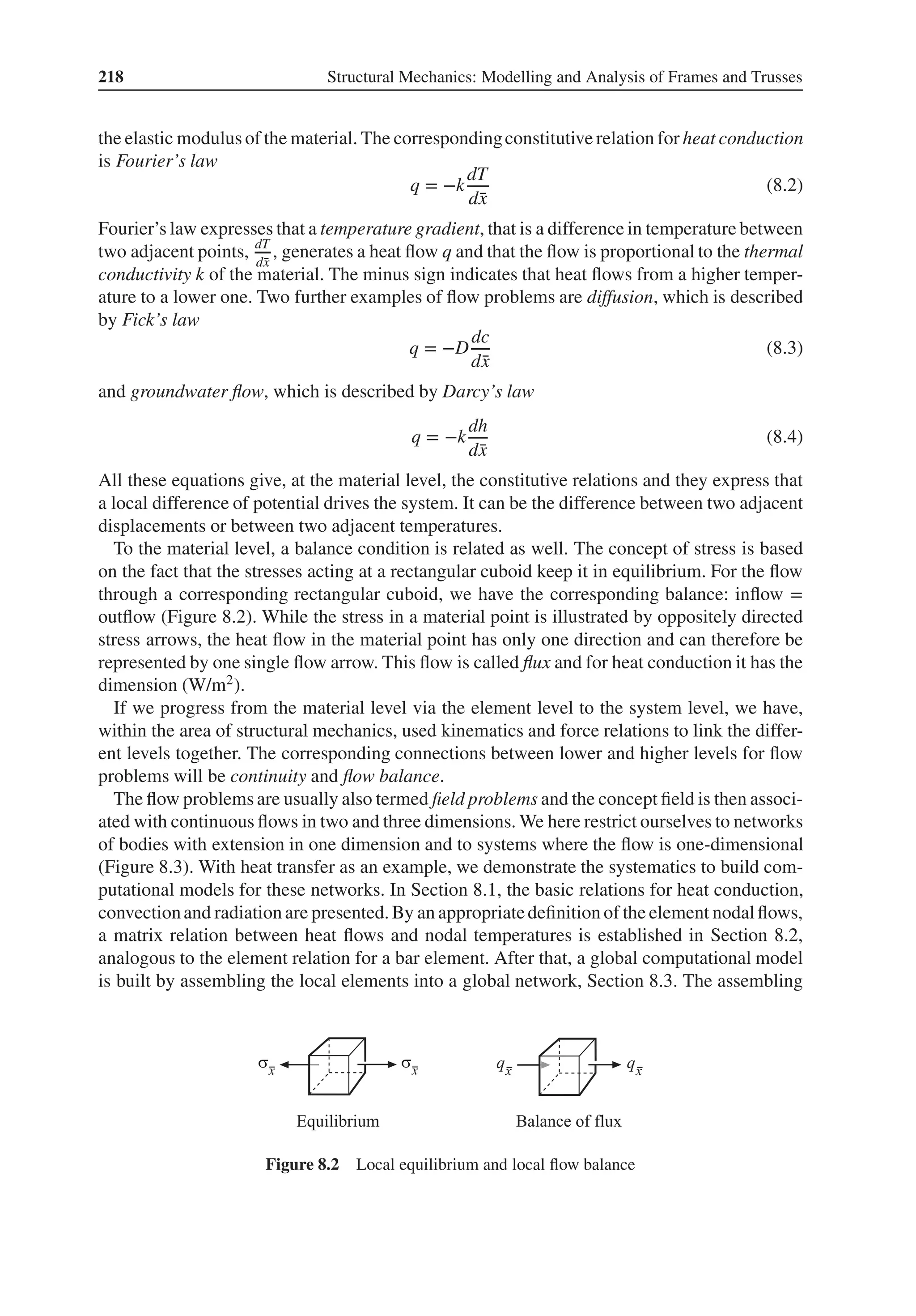
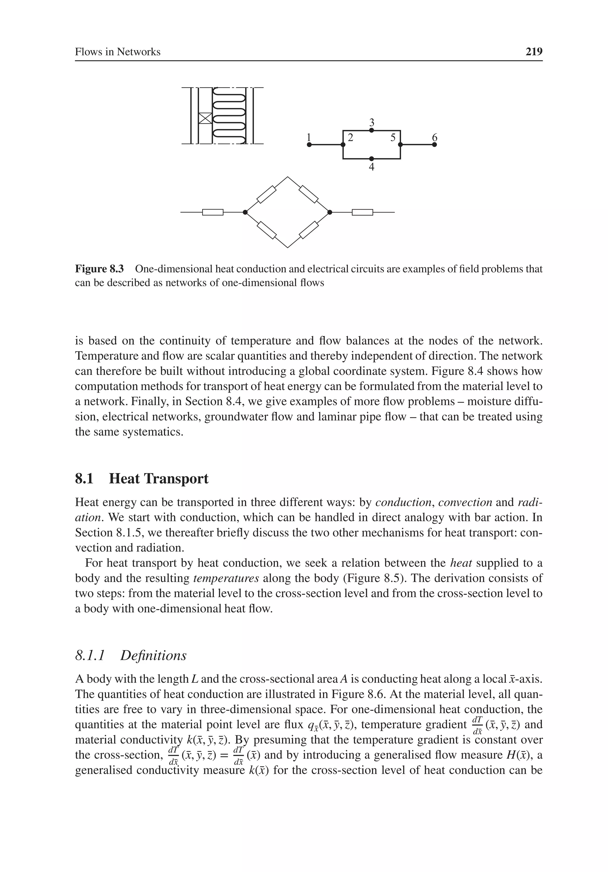
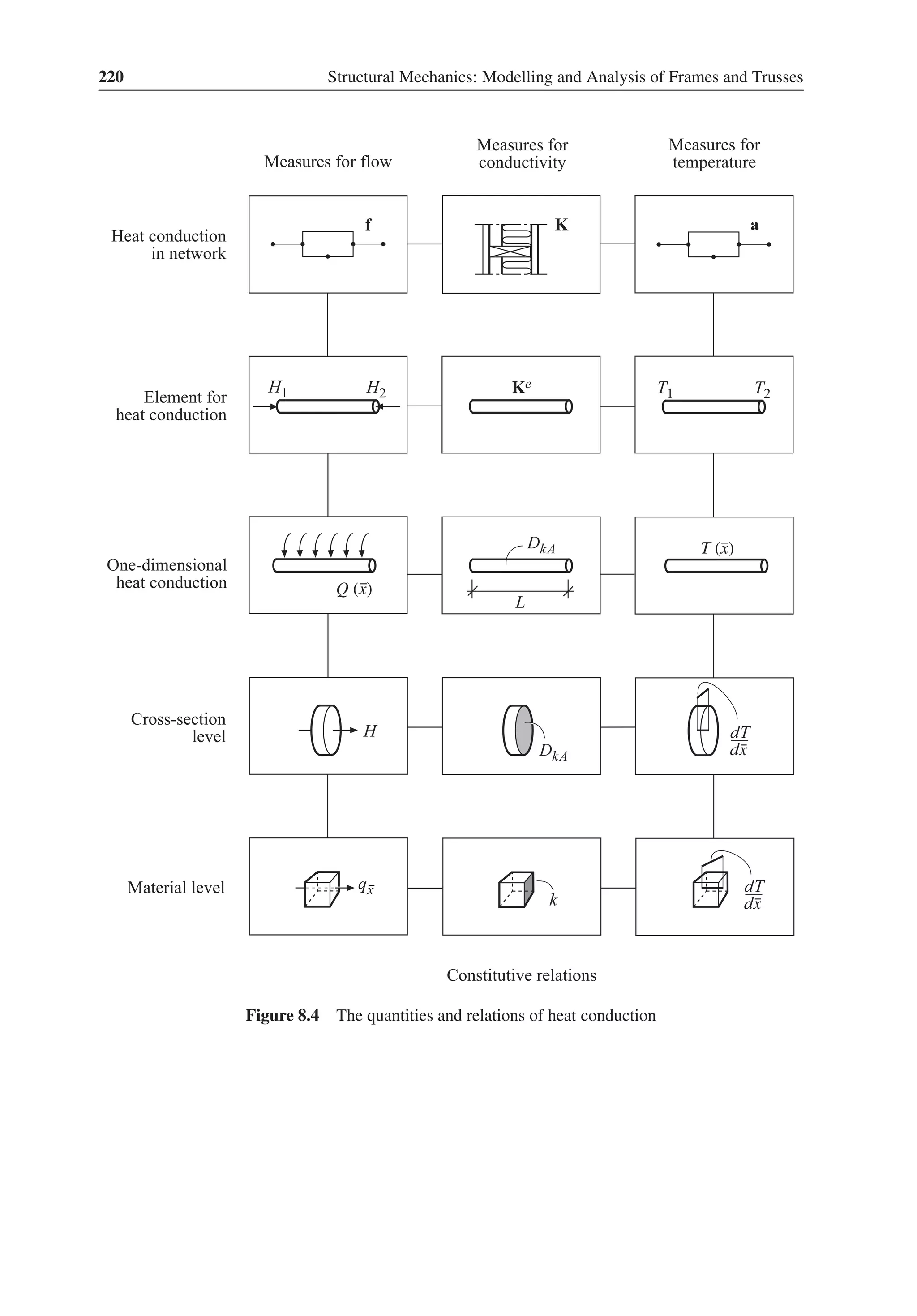
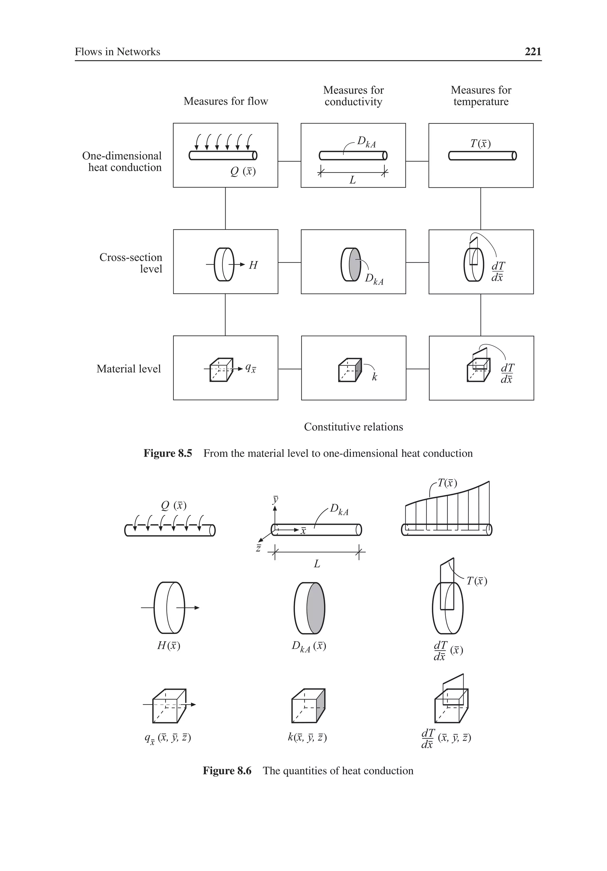
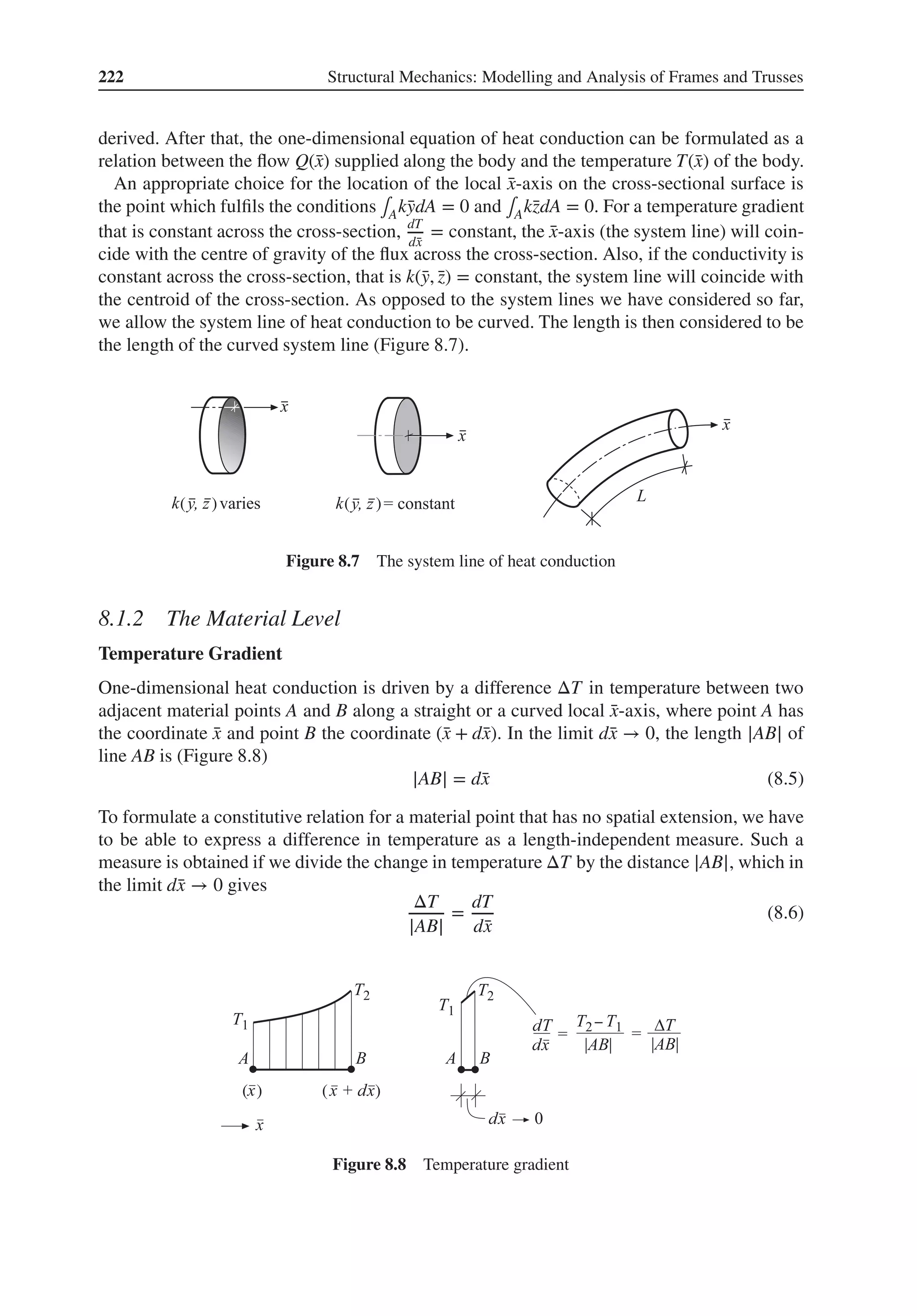
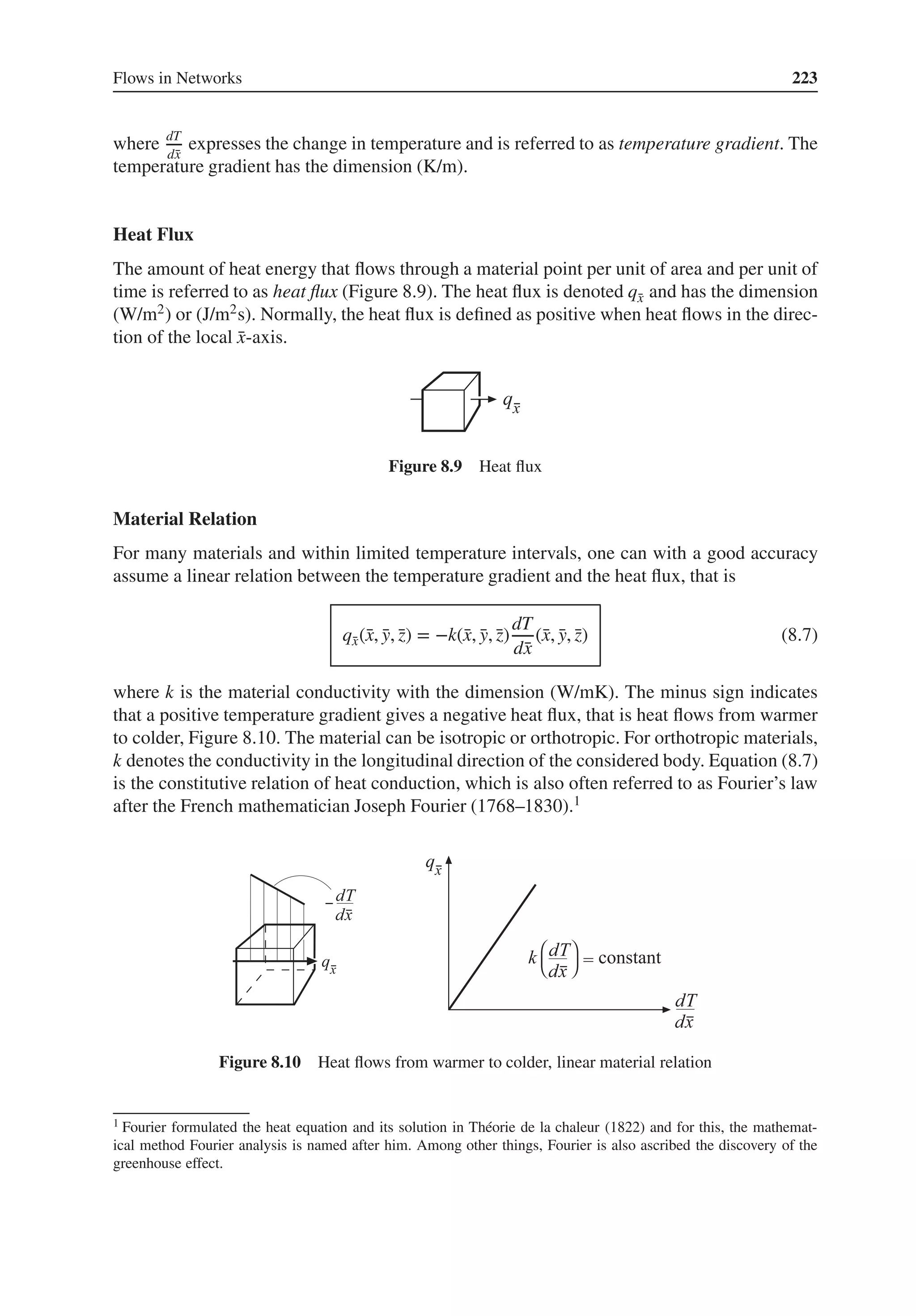
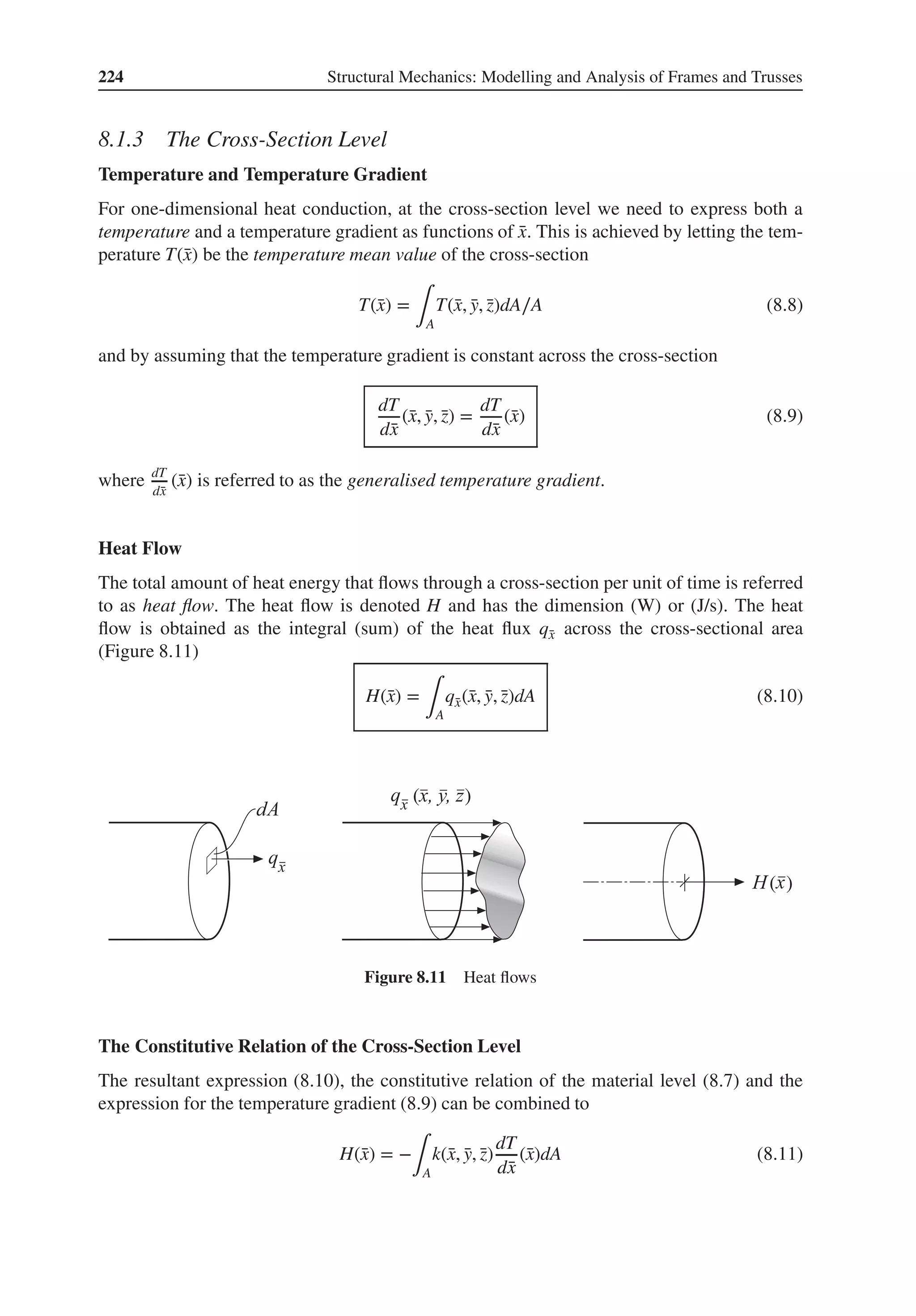
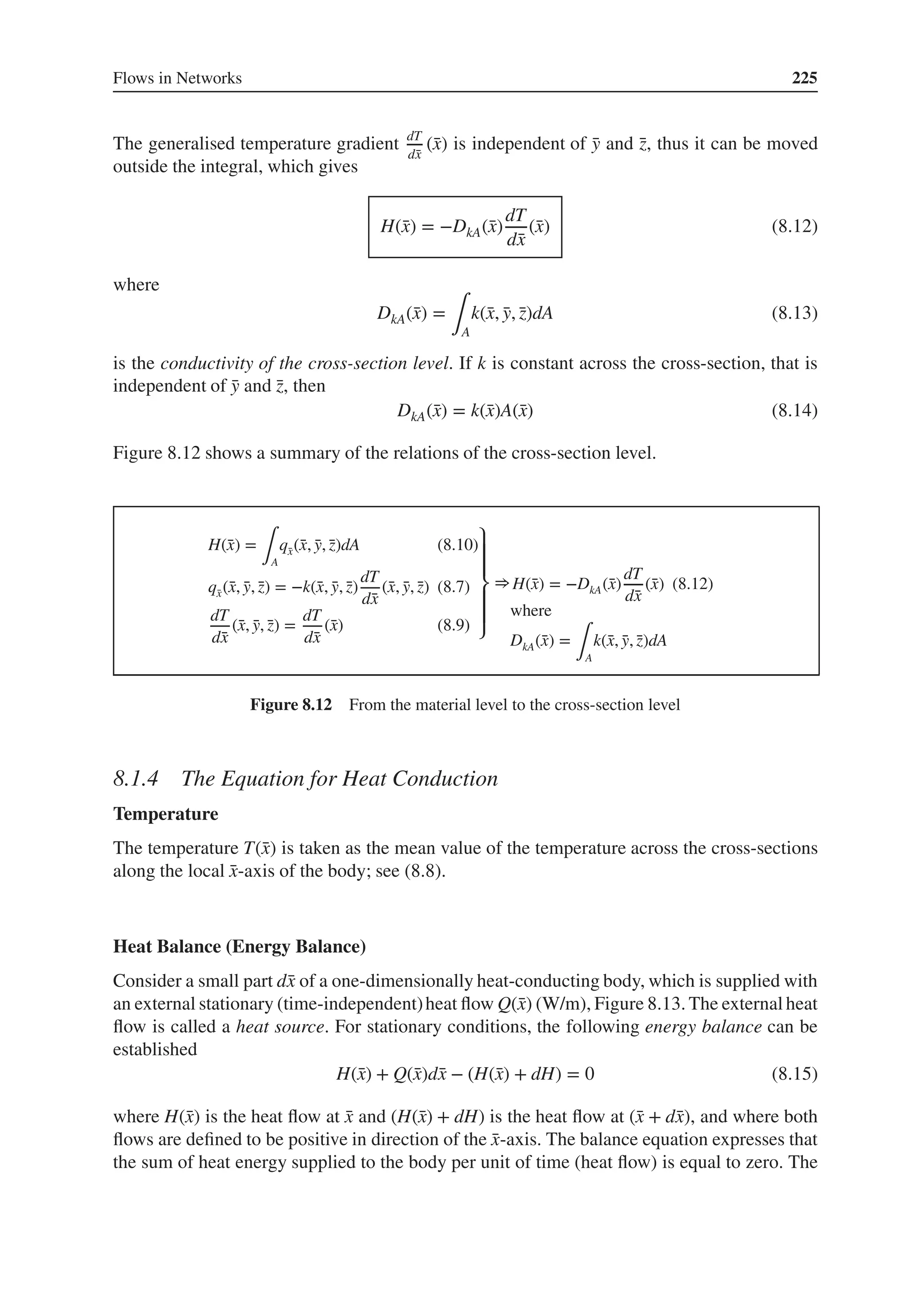
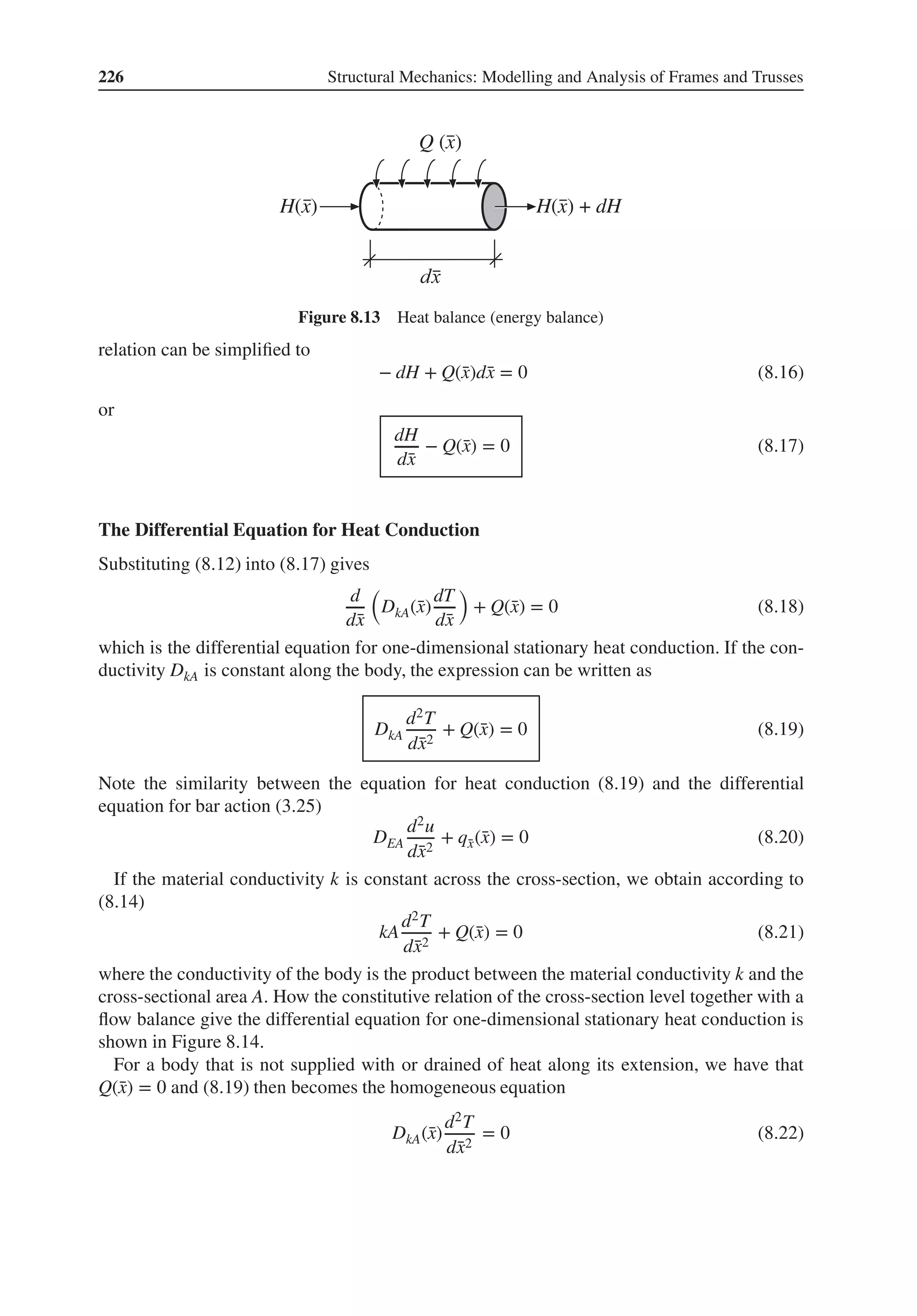
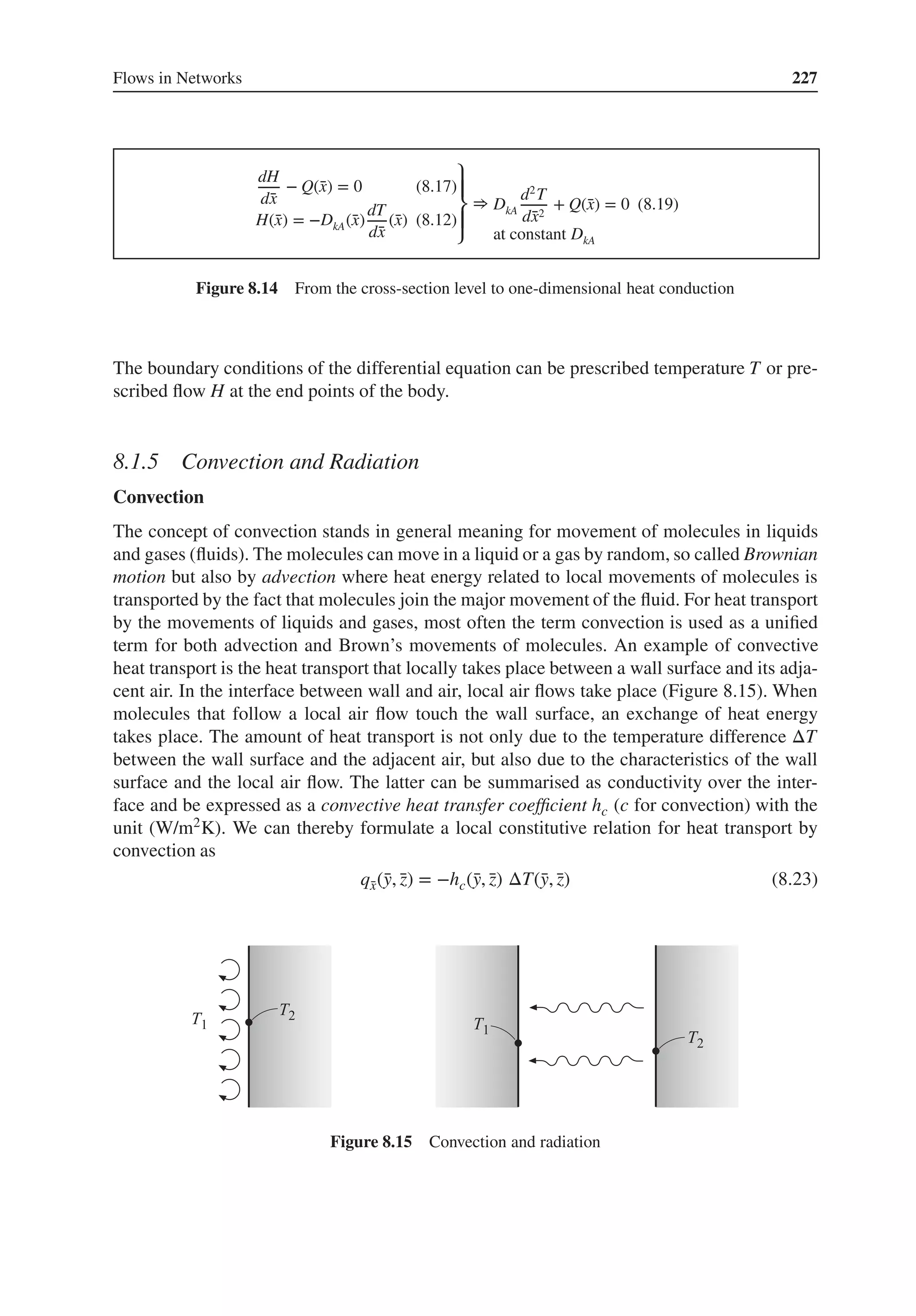
![228 Structural Mechanics: Modelling and Analysis of Frames and Trusses
where the temperature difference ΔT is positive for increasing temperature in the direction of
the local ̄
x-axis.
For a cross-section with the area A, we have the conductive heat flow H given by the integral
of the heat flux q̄
x according to (8.10). With the cross-section temperature T regarded as the
average temperature according to (8.8) and with hc(̄
y, ̄
z) = constant, we have
q̄
x = −hcΔT (8.24)
Substituting (8.24) into (8.10) the constitutive relation at the cross-section level can be writ-
ten as
H = −hc A ΔT (8.25)
Radiation
The third phenomenon for transport of heat energy is radiation. All bodies with a temperature
above absolute zero send out heat radiation. Heat radiation is an electromagnetic radiation
with different spectra of frequencies depending on the temperature of the body. The higher the
temperature is, the higher is the average frequency. It has been shown that the radiated flux is
proportional to the absolute temperature to the power of 4. The local constitutive relation for
heat radiation is formulated by Stefan–Boltzmann’s law as
q̄
x = 𝜀𝜎
(
T4
− T4
0
)
(8.26)
where q̄
x is the total radiated flux. T is the temperature of the radiating surface and T0 is the
temperature of the environment or an opposite surface given in Kelvin (K) (Figure 8.15). The
factor 𝜀 is a constant in the interval [0, 1] which describes the magnitude of the radiation. For
most bodies, the value 𝜀 = 1 is approximately used, which corresponds to an ideal black body.
The factor 𝜎 is called the Stefan–Boltzmann constant and has the value
𝜎 =
2𝜋5k4
B
15c2h3
= 5.67 × 10⁻⁸
(W/m2
K4
) (8.27)
where kB is the Boltzmann constant, c is the speed of light and h is the Planck constant.
By reformulation of the Stefan–Boltzmann law (8.26), we can formulate a constitutive rela-
tion for radiation analogous to Fourier’s law (8.7) and the constitutive relation for convective
heat transport (8.23). We have
(
T4
− T4
0
)
=
(
T2
+ T2
0
) (
T2
− T2
0
)
=
(
T2
+ T2
0
) (
T + T0
) (
T − T0
)
(8.28)
which means that (8.26) can be written as
q̄
x = 𝜀𝜎
(
T2
+ T2
0
) (
T + T0
) (
T − T0
)
(8.29)
or
q̄
x = −hrΔT (8.30)
where
hr = 𝜀𝜎
(
T2
+ T2
0
) (
T + T0
)
(8.31)
and where the temperature difference ΔT is positive for increasing temperature in the direction
of the local ̄
x-axis.](https://image.slidesharecdn.com/structuralmechanicsmodellingandanalysisofframesandtrussespdfdrive-230720064114-5e1f9a93/75/Structural-mechanics-_-modelling-and-analysis-of-frames-and-trusses-PDFDrive-pdf-242-2048.jpg)
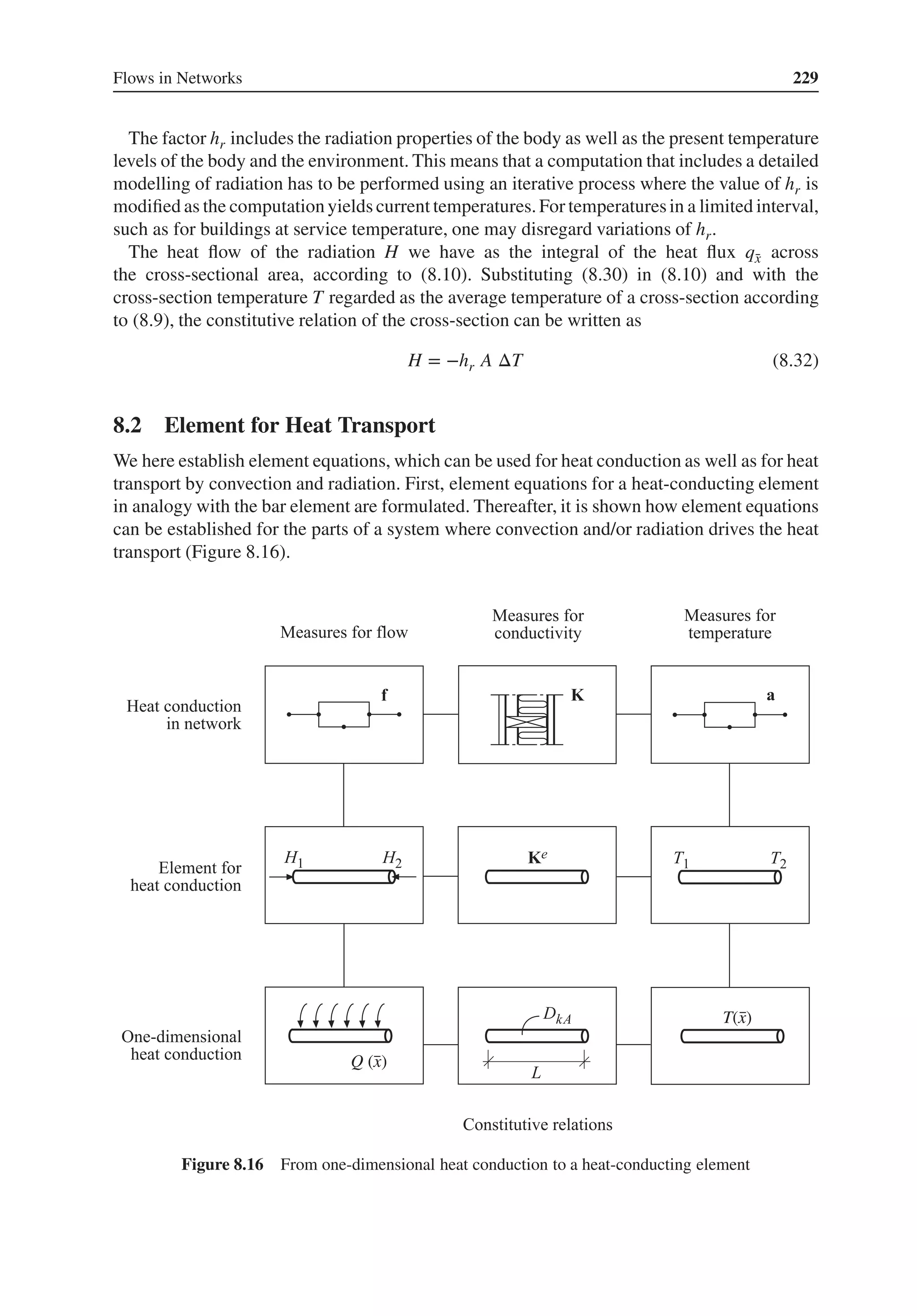
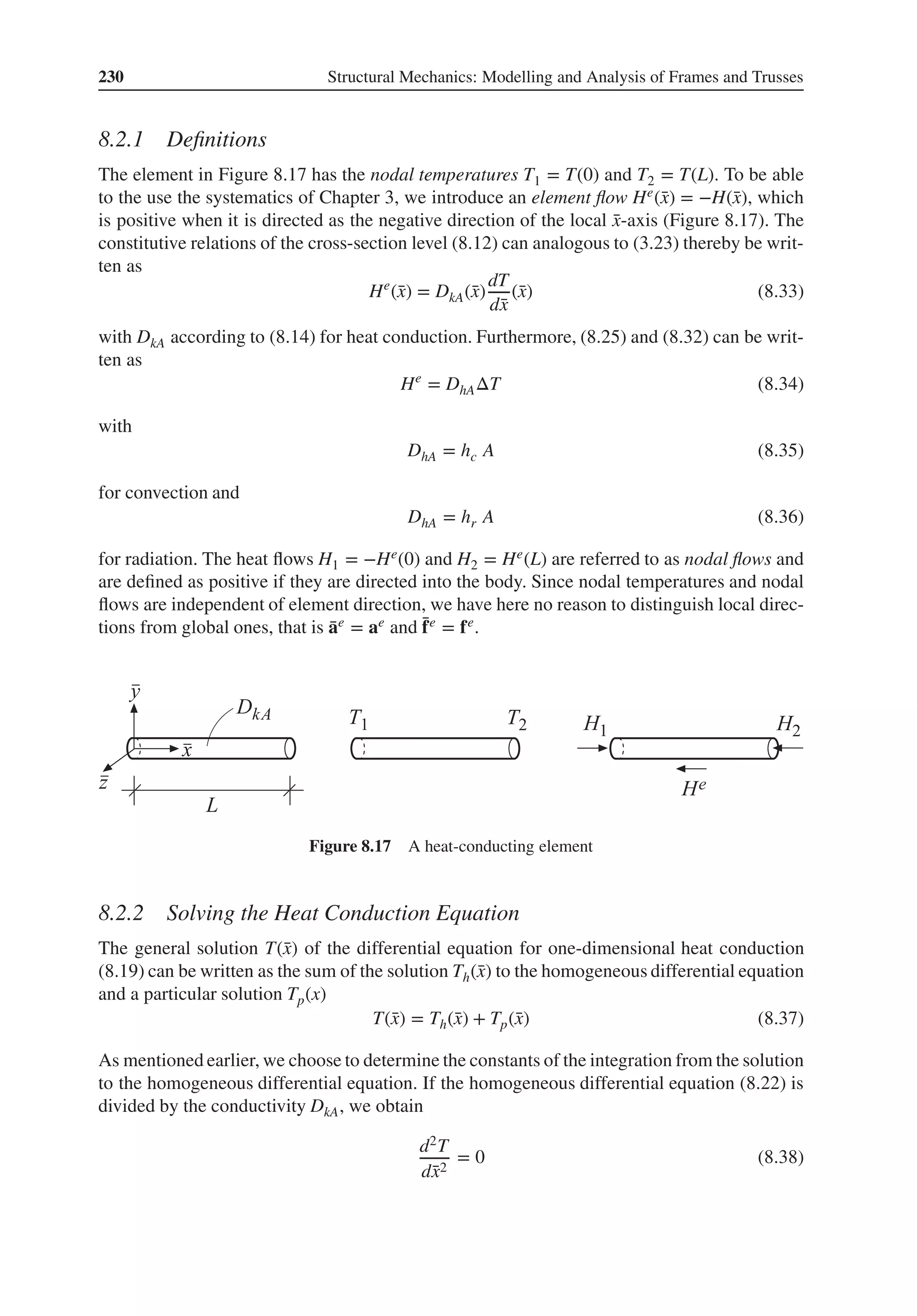
![Flows in Networks 231
Analogous to the derivation (3.29)–(3.43) we can find a solution Th(̄
x) to the homogeneous
differential equation that expresses the temperature variation along the element as a function
of the nodal temperatures of the element
Th(̄
x) = Nae
= N1(̄
x) T1 + N2(̄
x) T2 (8.39)
where
N =
[
1 − ̄
x
L
̄
x
L
]
; ae
=
[
T1
T2
]
(8.40)
The general solution to the differential equation is given by (8.37). Substituting (8.39) gives
T(̄
x) = Nae
+ Tp(̄
x) (8.41)
where the particular solution Tp(̄
x) is different for different types of supplied heat flow along
the heat-conducting element. The choice to, in (8.41), express the constants of integration as
functions of the nodal temperatures ae gives the condition that the particular solution may not
affect ae, that is
Tp(0) = 0 (8.42)
Tp(L) = 0 (8.43)
With this systematics, the general solution T(̄
x) can be understood as the sum of the temper-
ature distribution created by the nodal temperatures Th(̄
x) of the non-loaded element and the
temperature distribution created by a supplied heat flow along an element with a temperature
T = 0 at both its ends. Example 8.1 shows how the particular solution is obtained for a
heat-conducting element with a supplied heat flow that is constant along the element.
Differentiating (8.41) gives
dT
d̄
x
= Bae
+
dTp
d̄
x
(8.44)
where
B =
dN
d̄
x
=
d ̄
N
d̄
x
C−1
=
[
0 1
]
[
1 0
−1
L
1
L
]
=
1
L
[
−1 1
]
(8.45)
Substituting (8.44) into the expression for element flow (8.33) gives
He
(̄
x) = DkA
(
Bae
+
dTp
dx
)
(8.46)
or
He
(̄
x) = DkABae
+ Hp(̄
x) (8.47)
where
Hp(̄
x) = DkA
dTp
d̄
x
(8.48)
The definitions we have introduced for flows across the element ends (Figure 8.17) give
H1 = −He
(0); H2 = He
(L) (8.49)](https://image.slidesharecdn.com/structuralmechanicsmodellingandanalysisofframesandtrussespdfdrive-230720064114-5e1f9a93/75/Structural-mechanics-_-modelling-and-analysis-of-frames-and-trusses-PDFDrive-pdf-245-2048.jpg)
![232 Structural Mechanics: Modelling and Analysis of Frames and Trusses
Substituting (8.47) gives the nodal flows
He
(0) = DkABae
+ Hp(0) (8.50)
He
(L) = DkABae
+ Hp(L) (8.51)
With
fe
b =
[
H1
H2
]
; Ke
=
DkA
L
[
1 −1
−1 1
]
; fe
p =
[
−Hp(0)
Hp(L)
]
(8.52)
(8.50) and (8.51) can be written in matrix form
fe
b = Ke
ae
+ fe
p (8.53)
The left-hand side of the system of equations contains the nodal flows of the element fe
b
, that
is the flows that act on both the ends of the element. On the right-hand side, these flows are
divided into two parts. The product Keae gives the part of the flows that is generated by the
temperatures of the end points and the vector fe
p gives the part of the flows that is generated by
the along the element supplied heat flow, the heat source Q(̄
x). The division of the flows into
two parts is illustrated in Figure 8.18.
To prepare for a systematic handling of loads, we now introduce an element load vector fe
l
,
fe
l = −fe
p =
[
Hp(0)
−Hp(L)
]
(8.54)
where the components of fe
l
can be interpreted as resulting flows of the heat source Q(̄
x). These
resulting flows act on the nodes at the end points of the element (Figure 8.19).
( )
( )
( )
( )
Figure 8.18 Heat-conducting element in balance](https://image.slidesharecdn.com/structuralmechanicsmodellingandanalysisofframesandtrussespdfdrive-230720064114-5e1f9a93/75/Structural-mechanics-_-modelling-and-analysis-of-frames-and-trusses-PDFDrive-pdf-246-2048.jpg)
![Flows in Networks 233
( )
( )
Figure 8.19 Heat source and equivalent element loads
Thereby, we can write (8.53) as
Ke
ae
= fe
(8.55)
where
̄
fe
= ̄
fe
b + ̄
fe
l (8.56)
Equation (8.55) is the constitutive relation between nodal flows and temperatures for
a heat-conducting element. The relation is referred to as the element equation for a
heat-conducting element and Ke is the conductivity matrix of the element, ae its temperature
vector and fe its flow vector. The relations leading to the relation of the heat-conducting
element are summarised in Figure 8.20.
H1 = −He
(0) (8.49)
H2 = He
(L)
He
(̄
x) = DkA(̄
x)
dT
d̄
x
(8.33)
T(̄
x) = N̄
ae
+ Tp(̄
x) (8.41)
⎫
⎪
⎪
⎬
⎪
⎪
⎭
⇒ Ke
ae
= fe
(8.55)
where
fe
= fe
b
+ fe
l
Ke
=
DkA
L
[
1 −1
−1 1
]
; ae
=
[
T1
T2
]
fe
b
=
[
H1
H2
]
; fe
l
=
[
Hp(0)
−Hp(L)
]
Figure 8.20 From the cross-section level to element for one-dimensional heat-conduction
For a non-loaded element, that is for ̄
fe
l
= 𝟎, the temperature is described by the solution
to the homogeneous equation only. The case when the supplied heat is uniform is treated in
Example 8.1.
For heat transport through walls, the energy flow is modelled as heat conduction in the
solid materials, while the heat transport over air spaces and in the interface between the wall](https://image.slidesharecdn.com/structuralmechanicsmodellingandanalysisofframesandtrussespdfdrive-230720064114-5e1f9a93/75/Structural-mechanics-_-modelling-and-analysis-of-frames-and-trusses-PDFDrive-pdf-247-2048.jpg)
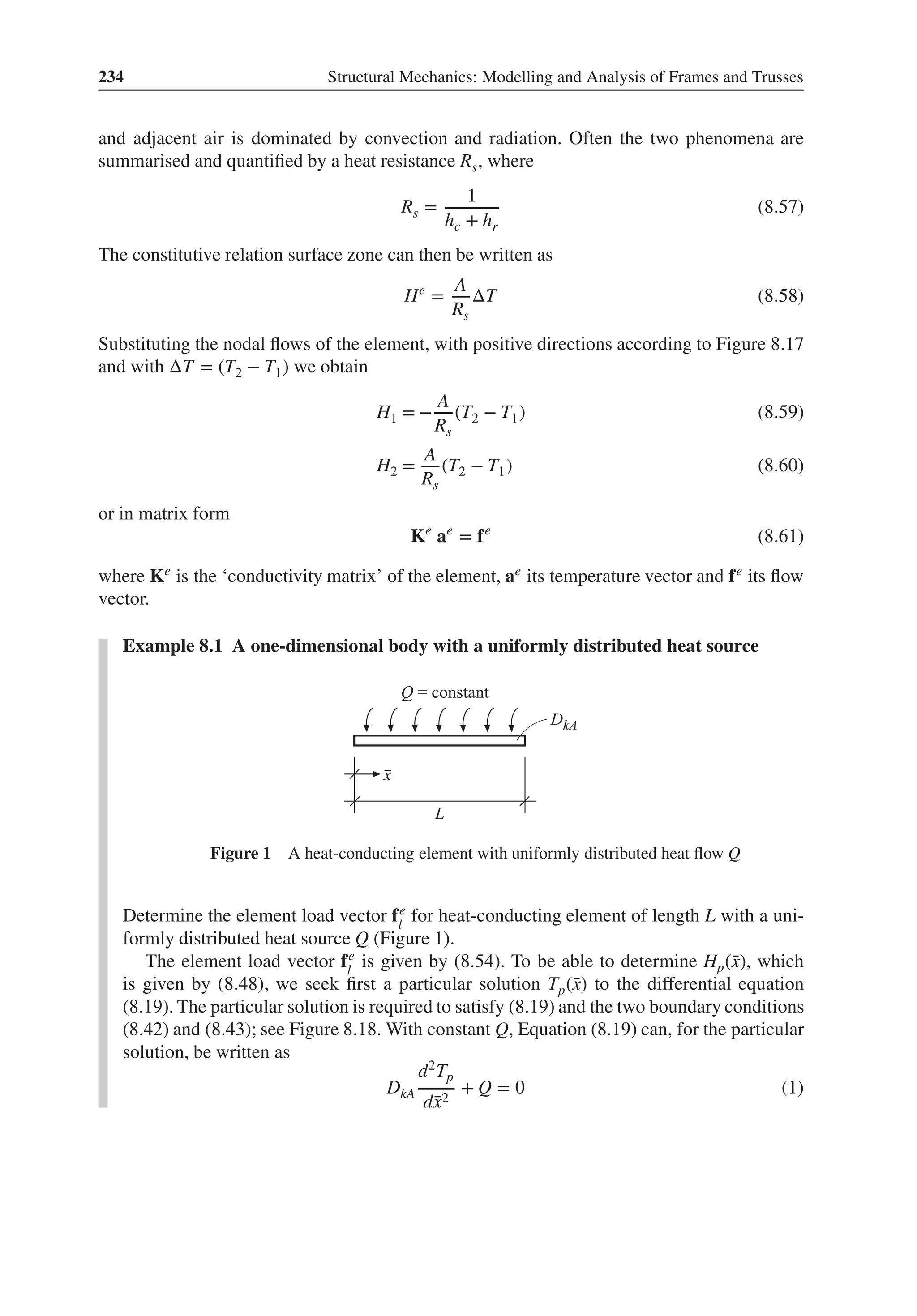
![Flows in Networks 235
Integration twice gives
DkA
dTp
d̄
x
+ Q̄
x − C1 = 0 (2)
DkATp(̄
x) + Q
̄
x2
2
− C1 ̄
x − C2 = 0 (3)
or
Tp(̄
x) =
1
DkA
(
−Q
̄
x2
2
+ C1 ̄
x + C2
)
(4)
The boundary conditions (8.42) and (8.43) give
Tp(0) =
1
DkA
C2 = 0; C2 = 0 (5)
Tp(L) =
1
DkA
(
−Q
L2
2
+ C1L + C2
)
= 0; C1 = Q
L
2
(6)
Substituting the constants C1 and C2, we obtain the particular solution
Tp(̄
x) = −
Q
DkA
(
̄
x2
2
−
L̄
x
2
)
(7)
Differentiation gives
dTp
d̄
x
= −
Q
DkA
(
̄
x −
L
2
)
(8)
which substituted into (8.48) gives
Hp(̄
x) = −Q
(
̄
x −
L
2
)
(9)
At the end points of the element, we have
Hp(0) = Q
L
2
; Hp(L) = −Q
L
2
(10)
Substituting Hp(0) and Hp(L) into (8.54), we obtain the element load vector
̄
fe
l =
QL
2
[
1
1
]
(11)
8.3 Networks of One-Dimensional Heat-Conducting Elements
A network consists of several one-dimensionalbodies connectedto each otherat the nodes. The
heat-conducting element we now have formulated is the basis for creation of a computational
model for a network.](https://image.slidesharecdn.com/structuralmechanicsmodellingandanalysisofframesandtrussespdfdrive-230720064114-5e1f9a93/75/Structural-mechanics-_-modelling-and-analysis-of-frames-and-trusses-PDFDrive-pdf-249-2048.jpg)
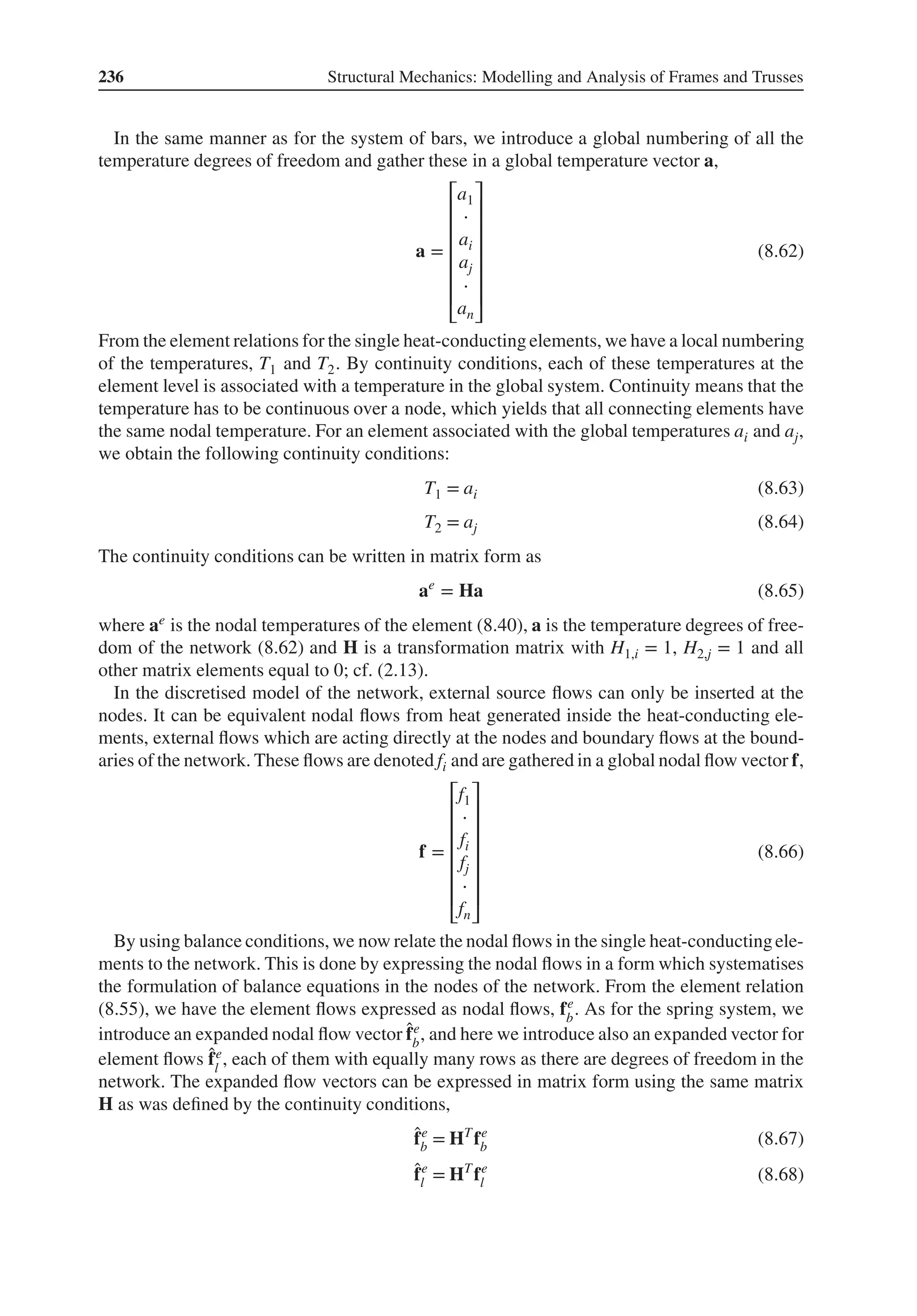
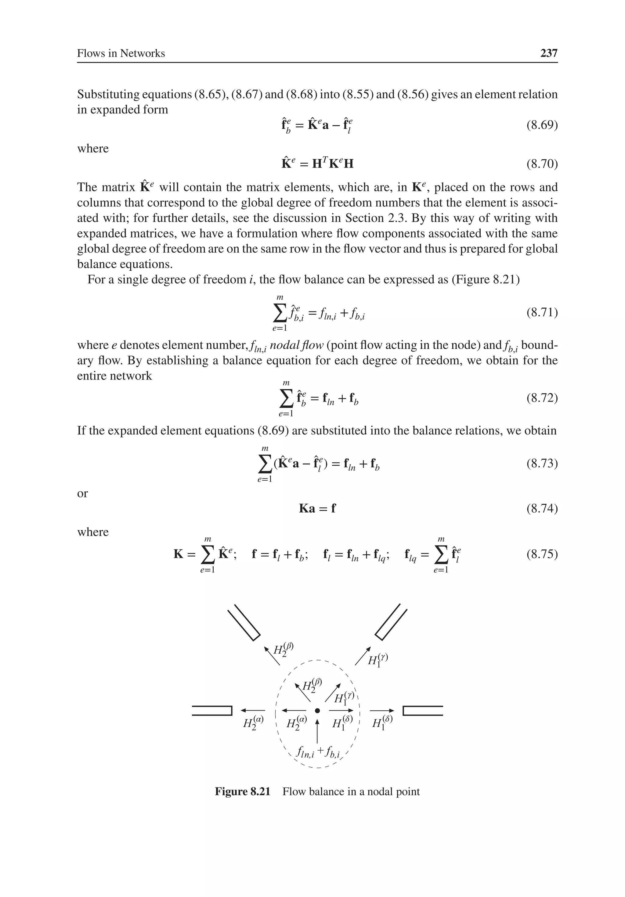
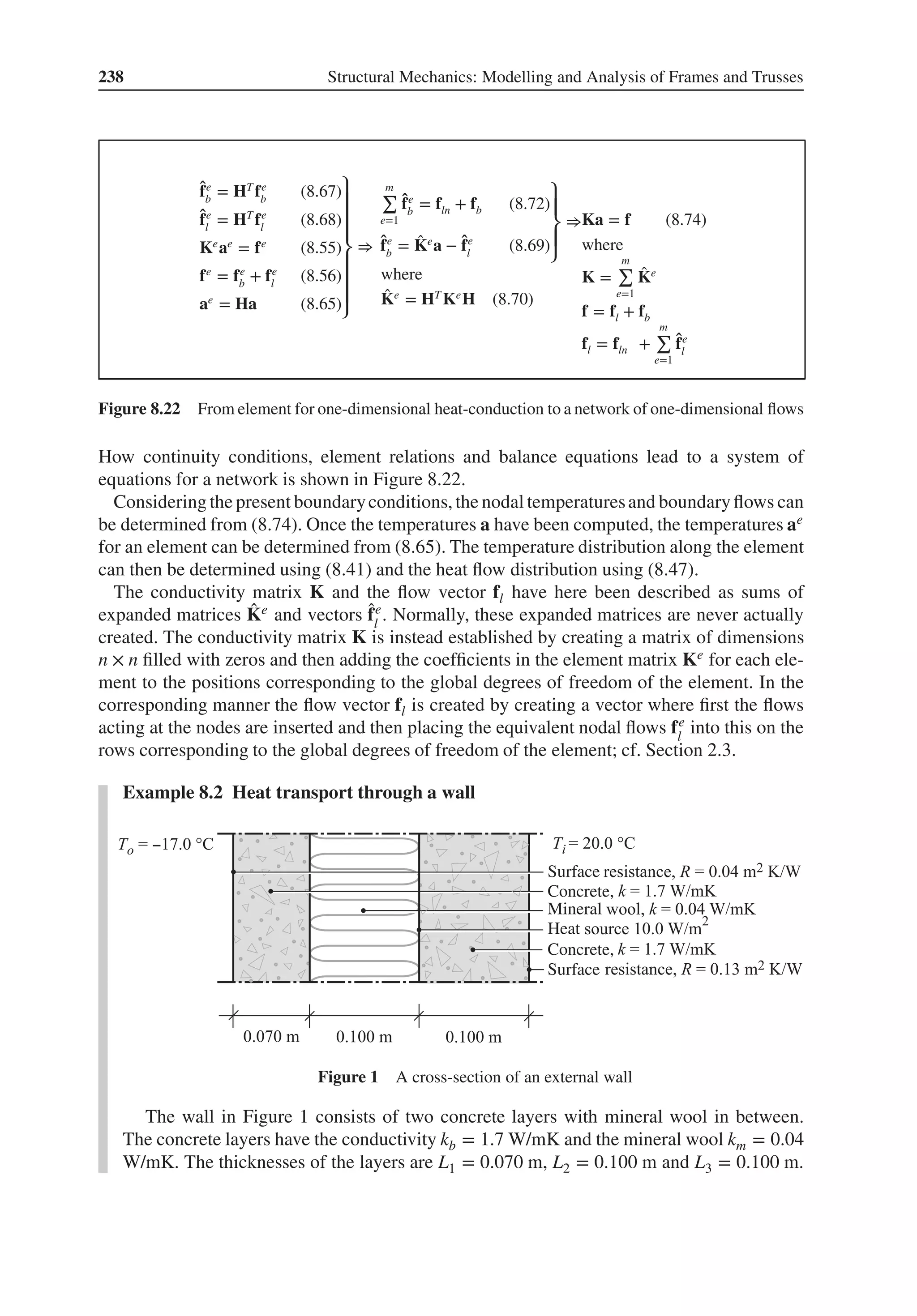
![Flows in Networks 239
The temperature on the outside of the wall is −17.0 ∘C and on the inside 20.0 ∘C. On the
outside, the thermal surface resistance is R = 0.04 m2 K/W and on the inside R = 0.13 m2
K/W. On the boundary between the mineral wool and the interior concrete layer, there is a
heat source that provides 10.0 W/m2. The temperature distribution and the stationary heat
flow through the wall shall be determined.
Computational model
Figure 2 Computational model
We choose to study the flow per m2 of the wall, that is we study 1 m2 wall. The wall is
modelled with five heat-conducting elements, denoted 1, 2, 3, 4 and 5, beginning from
the outside (Figure 2). Element 1 describes the thermal surface resistance on the outside,
Element 2 the exterior concrete layer, Element 3 the mineral wool, Element 4 the interior
concrete layer and Element 5 the interior thermal surface resistance. The model has tem-
perature degrees of freedom a1, a2, a3, a4, a5 and a6. The temperatures given on the outside
and on the inside imply that degrees of freedom a1 and a6 shall be prescribed to be −17
and 20 ∘C, respectively. The heat source inside the wall implies that fl,4 = 10 W/m2.
Element matrices
For each element, an element relation Keae = fe
l
+ fe
b
can be established. The element con-
ductivity matrix Ke is given by (8.52). For the five elements in our model, we have the
following:
Elements 2–4: With A, k and L known,the element conductivity matrix can be computed,
̄
K2
=
kA
L
[
1 −1
−1 1
]
=
1.7 ⋅ 1
0.07
[
1 −1
−1 1
]
= 24.3
[
1 −1
−1 1
]
(1)
̄
K3
=
0.04 ⋅ 1
0.1
[
1 −1
−1 1
]
= 0.4
[
1 −1
−1 1
]
(2)
̄
K4
=
1.7 ⋅ 1
0.1
[
1 −1
−1 1
]
= 17.0
[
1 −1
−1 1
]
(3)
Elements 1 and 5: These elements describe the thermal surface resistance between the wall
and the air.
̄
K1
=
A
Rs
[
1 −1
−1 1
]
=
1
0.04
[
1 −1
−1 1
]
= 25.0
[
1 −1
−1 1
]
(4)
̄
K5
=
1
0.13
[
1 −1
−1 1
]
= 7.7
[
1 −1
−1 1
]
(5)](https://image.slidesharecdn.com/structuralmechanicsmodellingandanalysisofframesandtrussespdfdrive-230720064114-5e1f9a93/75/Structural-mechanics-_-modelling-and-analysis-of-frames-and-trusses-PDFDrive-pdf-253-2048.jpg)
![240 Structural Mechanics: Modelling and Analysis of Frames and Trusses
Continuity conditions
The relation between the local degrees of freedom and the global degrees of freedom is
described by the topology matrix:
topology =
⎡
⎢
⎢
⎢
⎢
⎣
1 1 2
2 2 3
3 3 4
4 4 5
5 5 6
⎤
⎥
⎥
⎥
⎥
⎦
(6)
Assembling
Substituting the element conductivity matrices in a global conductivity matrix is performed
using the topology information,
K =
⎡
⎢
⎢
⎢
⎢
⎢
⎢
⎣
25.0 −25.0 0 0 0 0
−25.0 49.3 −24.3 0 0 0
0 −24.3 24.7 −0.4 0 0
0 0 −0.4 17.4 −17.0 0
0 0 0 −17.0 24.7 −7.7
0 0 0 0.0 −7.7 7.7
⎤
⎥
⎥
⎥
⎥
⎥
⎥
⎦
(7)
The heat source of 10.0 W/m2 inside the wall is placed on position 4 in the global flow
vector,
fl =
⎡
⎢
⎢
⎢
⎢
⎢
⎢
⎣
0
0
0
10.0
0
0
⎤
⎥
⎥
⎥
⎥
⎥
⎥
⎦
(8)
Boundary conditions
The temperature is prescribed in the degrees of freedom where the construction is in contact
with the air outside and with the air inside, that is a1 = −17.0, a6 = 20.0. This is described
by the boundary condition matrix
boundary conditions =
[
1 −17.0
6 20.0
]
(9)
In the degrees of freedom where the temperature is prescribed, boundary flows arise. These
are unknown for now and are denoted fb,1 and fb,6, respectively. The temperature vector a](https://image.slidesharecdn.com/structuralmechanicsmodellingandanalysisofframesandtrussespdfdrive-230720064114-5e1f9a93/75/Structural-mechanics-_-modelling-and-analysis-of-frames-and-trusses-PDFDrive-pdf-254-2048.jpg)
![Flows in Networks 241
and the boundary flow vector fb can now be written as
a =
⎡
⎢
⎢
⎢
⎢
⎢
⎢
⎣
−17.0
a2
a3
a4
a5
20.0
⎤
⎥
⎥
⎥
⎥
⎥
⎥
⎦
; fb =
⎡
⎢
⎢
⎢
⎢
⎢
⎢
⎣
fb,1
0
0
0
0
fb,6
⎤
⎥
⎥
⎥
⎥
⎥
⎥
⎦
(10)
Solving the system of equations
By solving the system of equations, we obtain
⎡
⎢
⎢
⎢
⎣
a2
a3
a4
a5
⎤
⎥
⎥
⎥
⎦
=
⎡
⎢
⎢
⎢
⎣
−16.44
−15.86
19.24
19.48
⎤
⎥
⎥
⎥
⎦
(11)
which means that the temperature at the surface of the wall is −16.44 ∘C and the tempera-
tures at the material boundaries are −15.86 and 19.24 ∘C, respectively, and the temperature
on the inside of the wall is 19.48 ∘C. We also obtain the boundary flows
[
fb,1
fb,6
]
=
[
−14.0
4.0
]
(12)
This means that we have the flow 14.0 W/m2 out of the wall on the outside and 4.0 W/m2
into the wall on the inside. We can conclude that the flows into the wall are −14.0 + 10.0 +
4.0 = 0, that is the external heat balance is satisfied.
Internal heat flows
With the global nodal temperatures a known, we can, using the continuity relations, deter-
mine the temperatures of each element
a1
=
[
−17.00
−16.44
]
(13)
a2
=
[
−16.44
−15.86
]
(14)
a3
=
[
−15.86
19.24
]
(15)
a4
=
[
19.24
19.48
]
(16)
a5
=
[
19.48
20.00
]
(17)](https://image.slidesharecdn.com/structuralmechanicsmodellingandanalysisofframesandtrussespdfdrive-230720064114-5e1f9a93/75/Structural-mechanics-_-modelling-and-analysis-of-frames-and-trusses-PDFDrive-pdf-255-2048.jpg)
![242 Structural Mechanics: Modelling and Analysis of Frames and Trusses
The flow through each element can be computed using (8.46). For Elements 1 and 5, k∕L
shall be replaced by 1∕R.
H(1)
=
1
0.04
[
−1 1
][
−17.00
−16.44
]
= 14.0 W (18)
H(2)
= 1.7
[
− 1
0.07
1
0.07
][
−16.44
−15.86
]
= 14.0 W (19)
H(3)
= 0.04
[
− 1
0.1
1
0.1
][
−15.86
19.24
]
= 14.0 W (20)
H(4)
= 1.7
[
− 1
0.1
1
0.1
][
19.24
19.48
]
= 4.0 W (21)
H(5)
=
1
0.13
[
−1 1
][
19.48
20.00
]
= 4.0 W (22)
8.4 Analogies
The above-described methodology for the analysis of systems of heat-conducting bodies has
several analogous applications and we briefly discuss the following areas: diffusion, laminar
liquid flow in pipes, groundwater flow and electric circuits. The analogies presented have been
limited to a description of steady-state (time-independent) processes.
8.4.1 Diffusion – Fick’s Law
The physical concept of diffusion describes a process where differences in concentration
decrease. The term concentration can refer to the matter itself (particles or molecules) and the
motion of the matter (thermal energy). In Sections 8.1 and 8.2, in the concept of diffusion,
we have studied how thermal energy is transported from hot (high concentration of molecular
motion) to cold (low concentration of molecular motion). In a more limited sense, the concept
of diffusion is used for description of the transport of substances where the transport is driven
by differences in concentration between adjacent regions. With that meaning, Fick’s first law
was formulated in the year 1855 by the German physiologist Adolf Fick (1829–1901)
J = −D
dc
d̄
x
(8.76)
where c denotes a concentration that either can be a density of mass (kg/m3) or an amount of
substance (mol/m3), D is the diffusivity (m2/s) of the material J indicates a flux of matter per
unit of area and unit of time (kg/m2s) or a flux of substance per unit of area and unit of time
(mol/m2s). One common application for buildings is vapour diffusion driven by differences in
concentration of vapour.
During a stationary (independent of time) process, the sum of all matter supplied to a delim-
ited body is equal to zero. No matter is created nor disappears uncontrolled during the process.
If we choose to consider the matter as density of mass and consider, analogous to Figure 8.13,
a one-dimensional body with the length d̄
x and the cross-sectional area A(̄
x), such a balance](https://image.slidesharecdn.com/structuralmechanicsmodellingandanalysisofframesandtrussespdfdrive-230720064114-5e1f9a93/75/Structural-mechanics-_-modelling-and-analysis-of-frames-and-trusses-PDFDrive-pdf-256-2048.jpg)
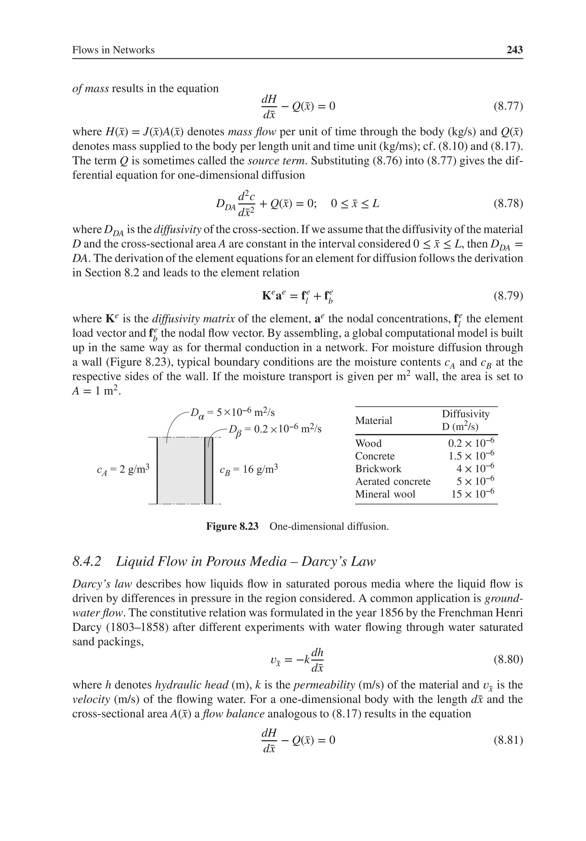
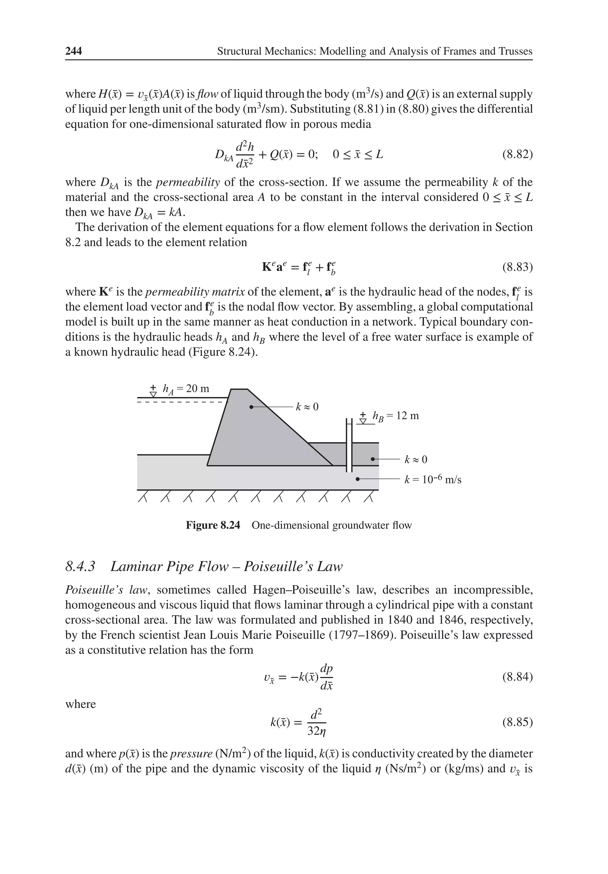
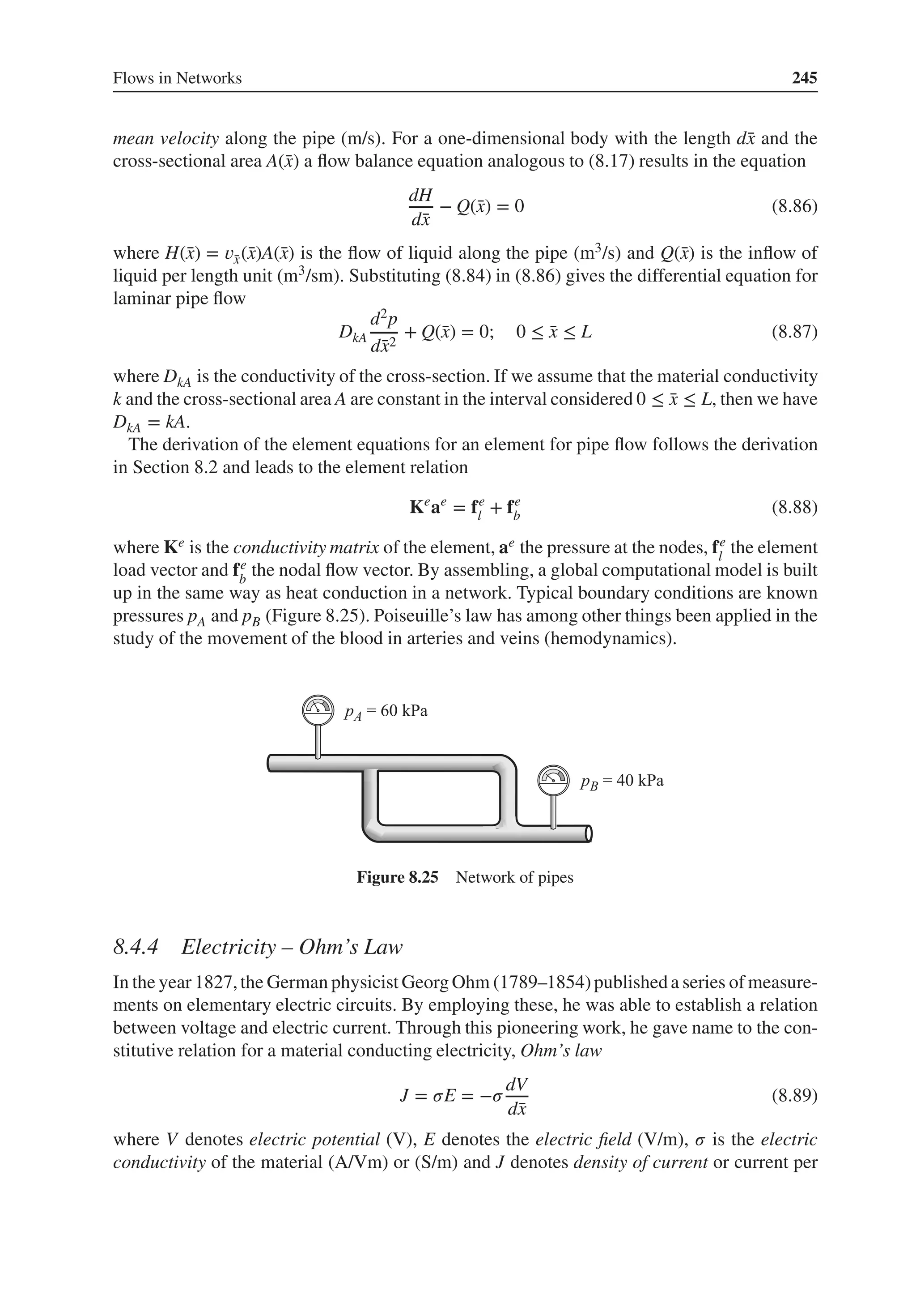
![246 Structural Mechanics: Modelling and Analysis of Frames and Trusses
unit of area (A/m2). A maybe more well-known form of Ohm’s law we have when we go up
in scale and consider a one-dimensional body conducting electricity
I = −
1
R
U (8.90)
where U denotes voltage (V), R is the resistance of the body [Ω] and I denotes electric cur-
rent (A).
An element conducting electricity (resistor) has as nodal variables electric potentials V1 and
V2 and nodal flows (currents) I1 and I2. The voltage U over an element is the difference in
electric potential U = V2 − V1; cf. (2.2). If we introduce Ie = −I (cf. Section 8.2), Ohm’s law
(8.90) for the element can be written as
Ie
=
1
R
(
V2 − V1
)
(8.91)
With the nodal flows of the element substituted and with positive directions according to
Figure 8.17, we get
I1 = −
1
R
(
V2 − V1
)
(8.92)
I2 =
1
R
(
V2 − V1
)
(8.93)
or, in matrix form
Ke
ae
= fe
b (8.94)
where Ke is the conductivity matrix of the element, ae the electric potential of the nodes and fe
b
the nodal flow vector. A global computational model is assembled in the same manner as heat
conduction in a network. Boundary conditions in electric circuits (Figure 8.26) can be known
electric potentials VA and VB and known currents IC. If a node in the circuit is connected to the
ground, this node has electric potential zero, that is the boundary condition VJ = 0.
Figure 8.26 Electric circuit
8.4.5 Summary
In Table 8.1, a summary is given of constitutive relations for the different areas of applied
mechanics, which have been treated.](https://image.slidesharecdn.com/structuralmechanicsmodellingandanalysisofframesandtrussespdfdrive-230720064114-5e1f9a93/75/Structural-mechanics-_-modelling-and-analysis-of-frames-and-trusses-PDFDrive-pdf-260-2048.jpg)
![Flows in Networks 247
Table 8.1 Summary of constitutive relations for different problem areas of applied mechanics
Physical problem Material level Cross-section level Differential equation
Bar Hooke’s law 𝜎̄
x = E du
d̄
x
N(̄
x) = DEA
du
d̄
x
DEA
d2u
d̄
x2
+ q̄
x(̄
x) = 0
Heat conduction Fourier’s law q̄
x = −kdT
d̄
x
H(̄
x) = −DkA
dT
d̄
x
DkA
d2T
d̄
x2
+ Q(x) = 0
Diffusion Fick’s law J = −Ddc
d̄
x
H(̄
x) = −DDA
dc
d̄
x
DDA
d2c
d̄
x2
+ Q(̄
x) = 0
Groundwater flow Darcy’slaw q̄
x = −kdh
d̄
x
H(̄
x) = −DkA
dh
d̄
x
DkA
d2h
d̄
x2
+ Q(̄
x) = 0
Laminar pipe flow Poiseuille’s law 𝑣̄
x = −kdp
d̄
x
H(̄
x) = −DkA
dp
d̄
x
DkA
d2p
d̄
x2
+ Q(̄
x) = 0
Spring N = k𝛿
Electric circuit Ohm’s law J = −𝜎 dV
d̄
x
I = 1
R
U
Exercises
8.1 In the figures, elements for modelling five different physical problems are shown. All of
them can be described by the same type of element matrix
Ke
= K
[
1 −1
−1 1
]
where K denotes the stiffness or conductivity of the element. Give a value of K for each
of the following elements:
(a) Spring
k = 8000 MN/m
(b) Bar
E = 21 GPa
A = 0.04 m2
(c) One-dimensional heat conduction
k = 0 .30 W/mK
(d) Heat resistance at boundary surface
Rs = 0 .04 m2
K/W](https://image.slidesharecdn.com/structuralmechanicsmodellingandanalysisofframesandtrussespdfdrive-230720064114-5e1f9a93/75/Structural-mechanics-_-modelling-and-analysis-of-frames-and-trusses-PDFDrive-pdf-261-2048.jpg)
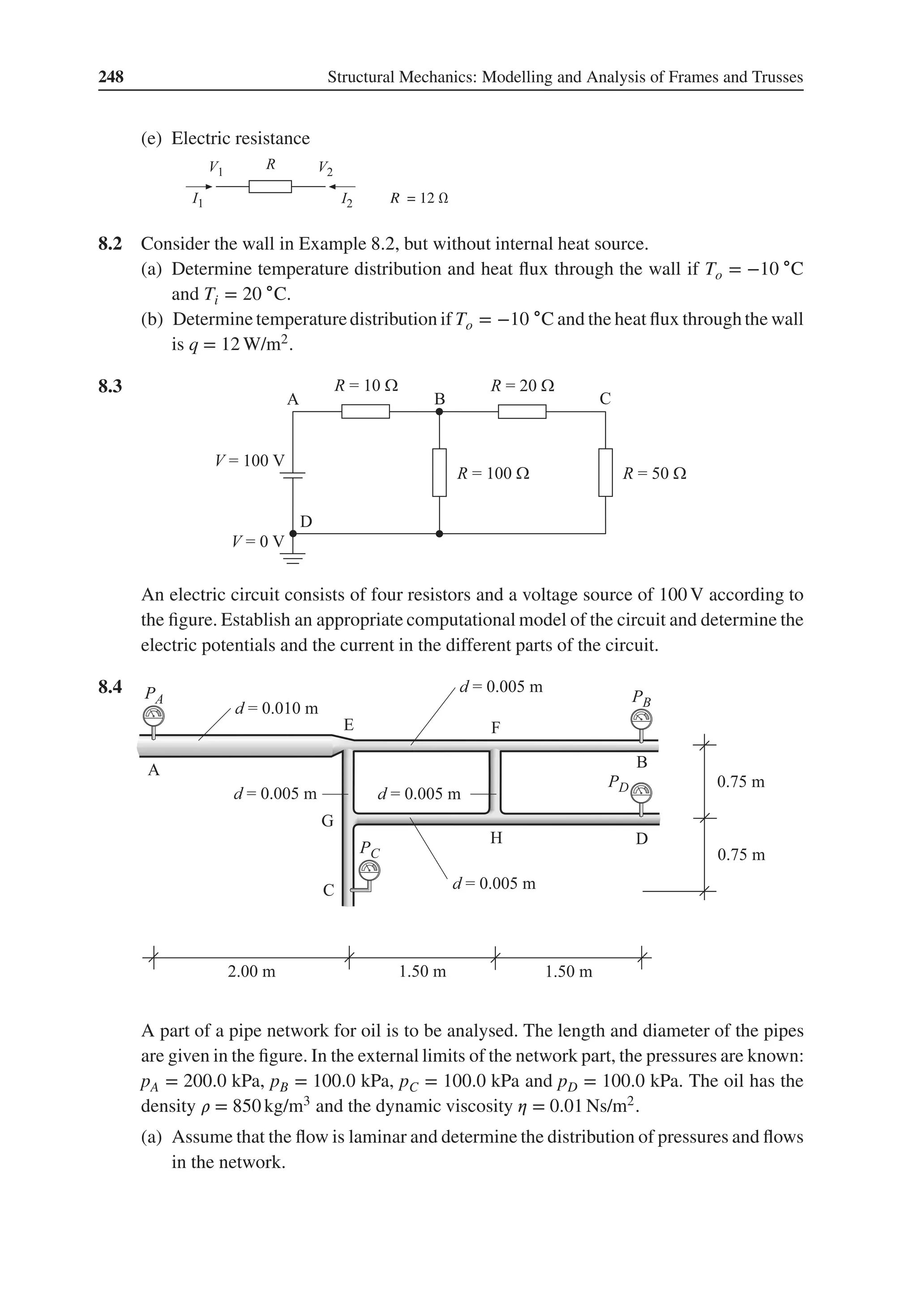
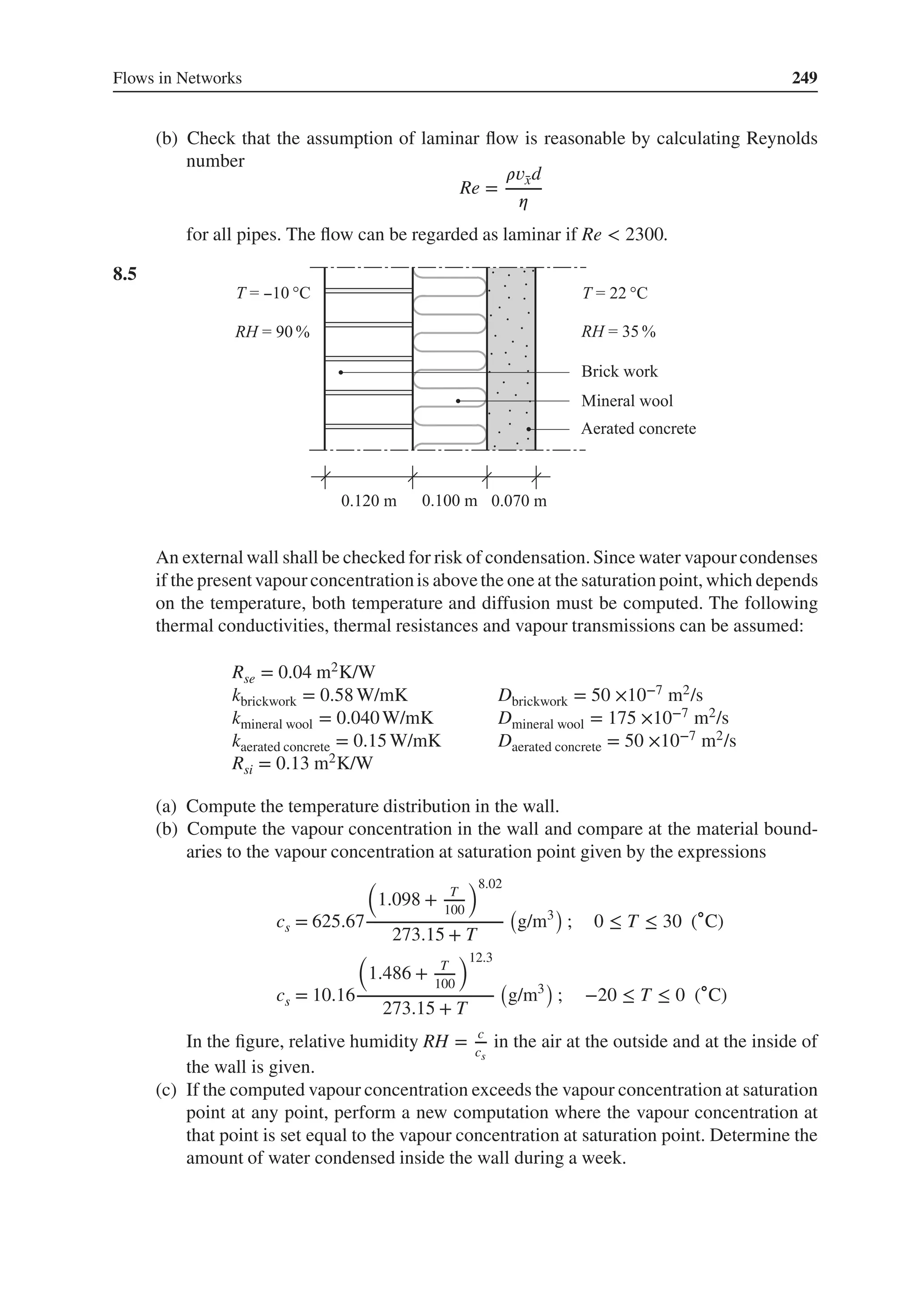

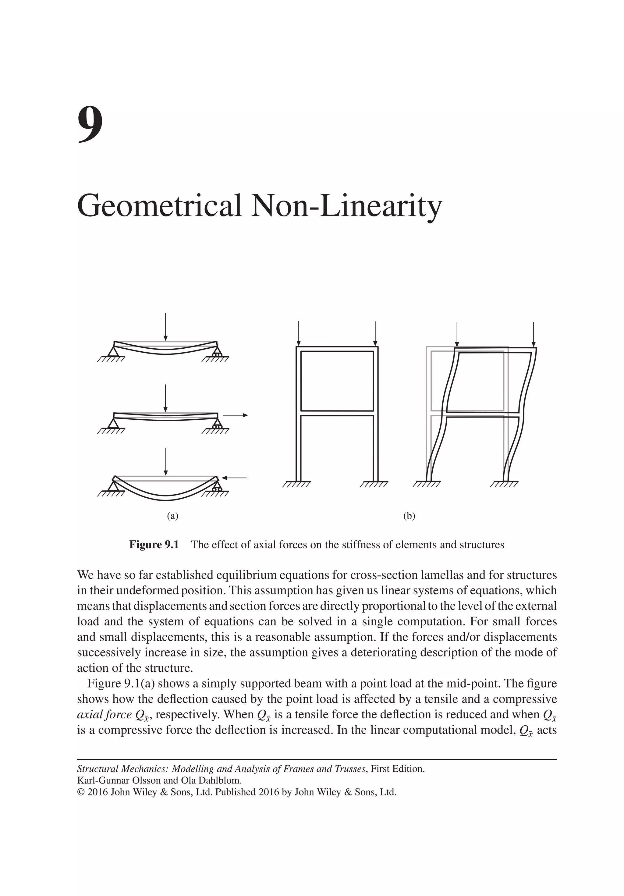
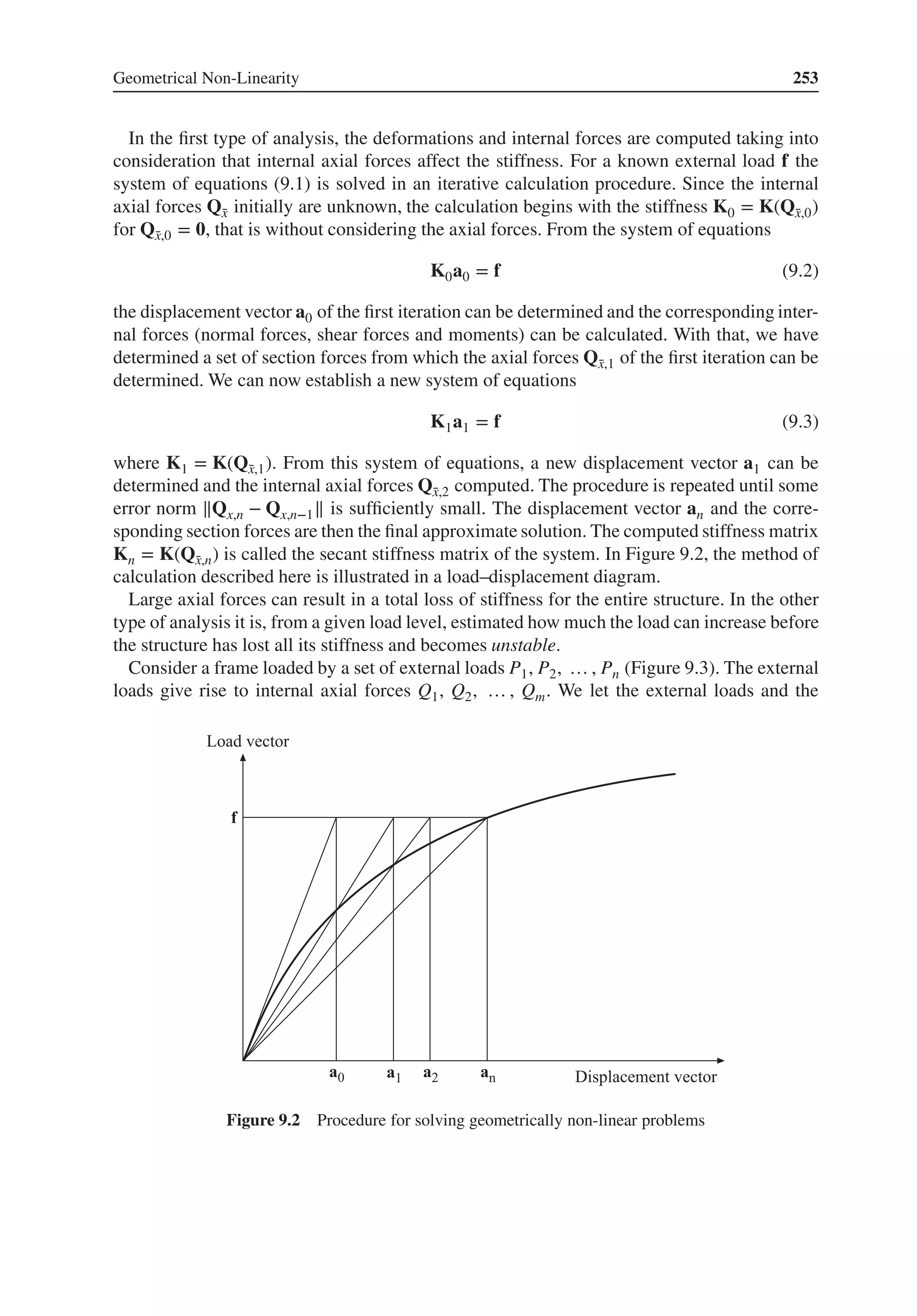
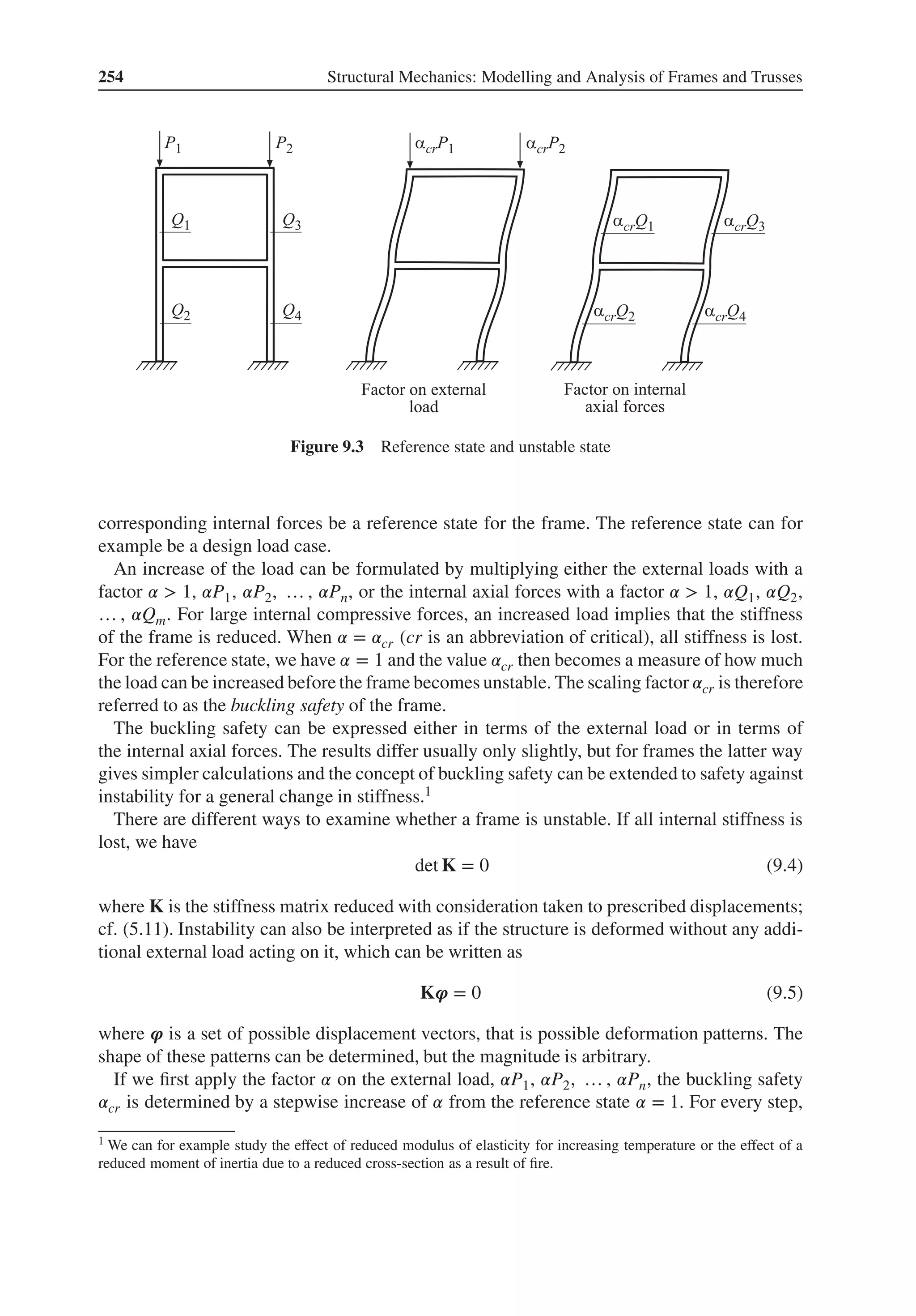
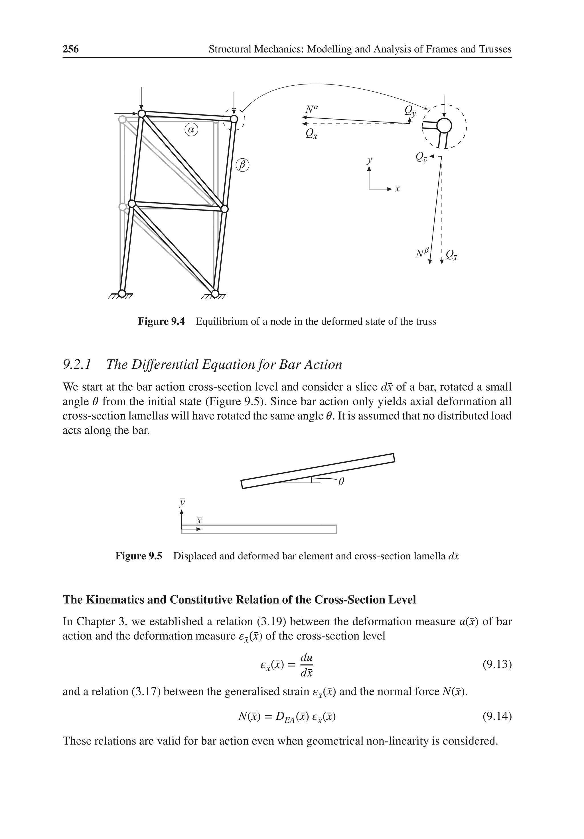
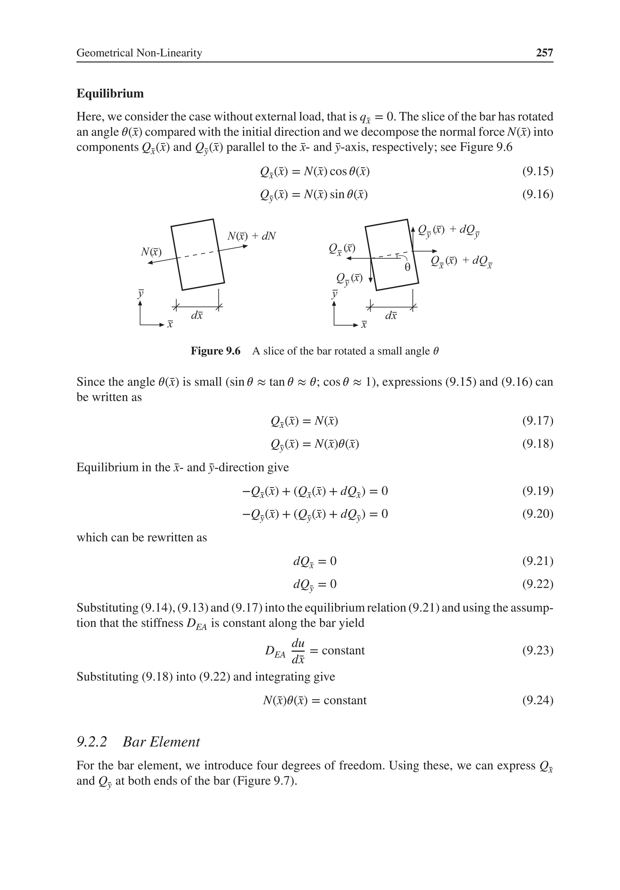
![258 Structural Mechanics: Modelling and Analysis of Frames and Trusses
Figure 9.7 Bar element and degrees of freedom
Solving the Differential Equation
From Chapter 3, we know that the solution of (9.23) can be expressed in terms of the nodal
displacements, denoted here by ̄
u1 and ̄
u3,
u(̄
x) = N̄
ae
=
[
1 − ̄
x
L
̄
x
L
][
̄
u1
̄
u3
]
(9.25)
Using (9.13) and substituting into (9.14) enable us to express the normal force using nodal
displacements
N = DEA
[
−1
L
1
L
][
̄
u1
̄
u3
]
(9.26)
Substitution into (9.17) gives the force component in the ̄
x-direction, Q̄
x
Q̄
x = DEA
[
−1
L
1
L
][
̄
u1
̄
u3
]
(9.27)
For pure bar action, the angle 𝜃 is constant along the element and can be expressed as a function
of the nodal displacements, ̄
u2 and ̄
u4, and the length L of the bar; see Figure 9.8
𝜃 ≈ sin 𝜃 =
̄
u4 − ̄
u2
L
(9.28)
With 𝜃 being constant, we obtain from (9.24) that N is constant. When considering this and
substituting (9.28) and (9.17) into (9.18), we obtain the force component in the ̄
y-direction, Q̄
y
Q̄
y = Q̄
x
[
−1
L
1
L
][
̄
u2
̄
u4
]
(9.29)
Figure 9.8 Displaced bar element](https://image.slidesharecdn.com/structuralmechanicsmodellingandanalysisofframesandtrussespdfdrive-230720064114-5e1f9a93/75/Structural-mechanics-_-modelling-and-analysis-of-frames-and-trusses-PDFDrive-pdf-272-2048.jpg)
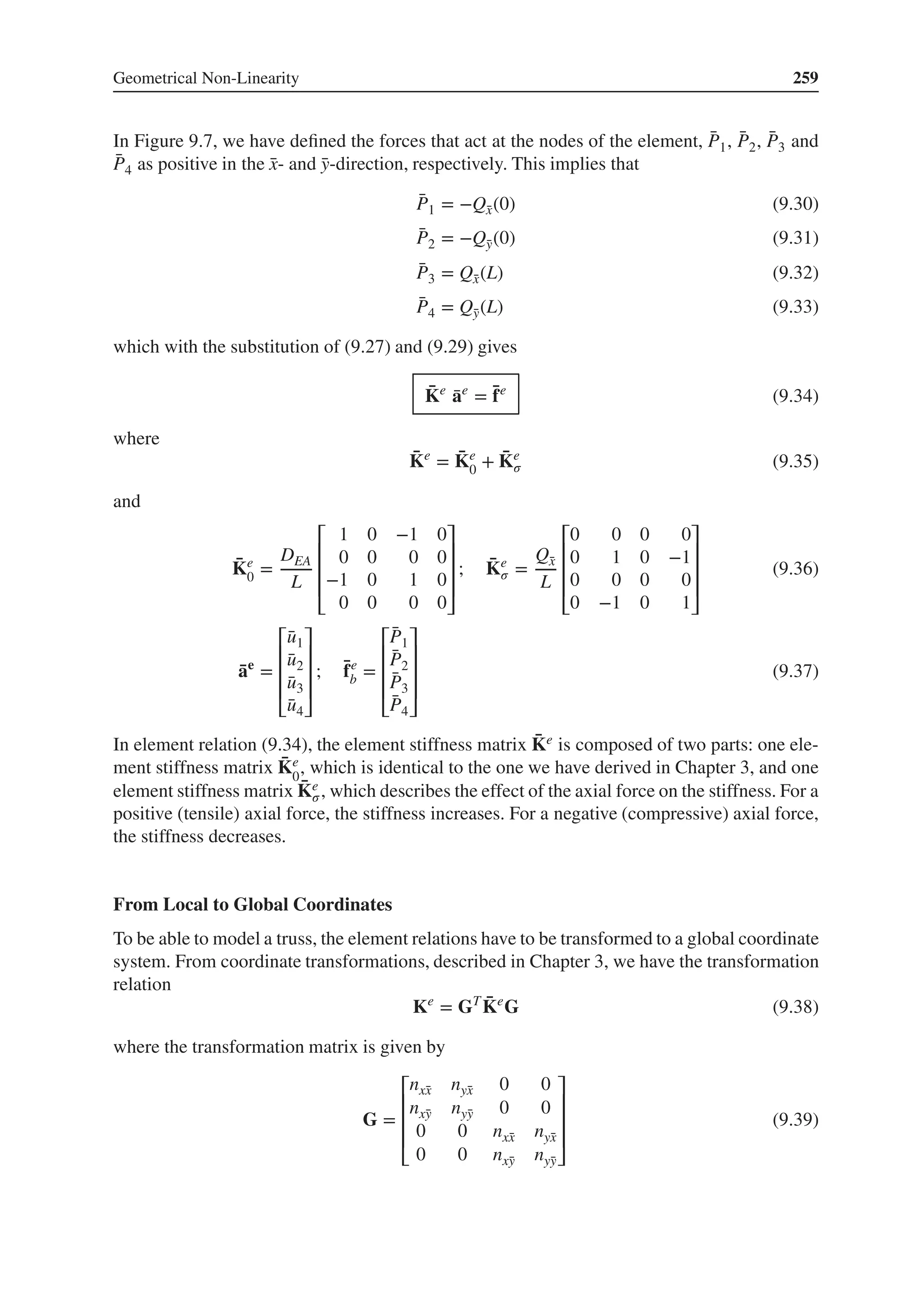
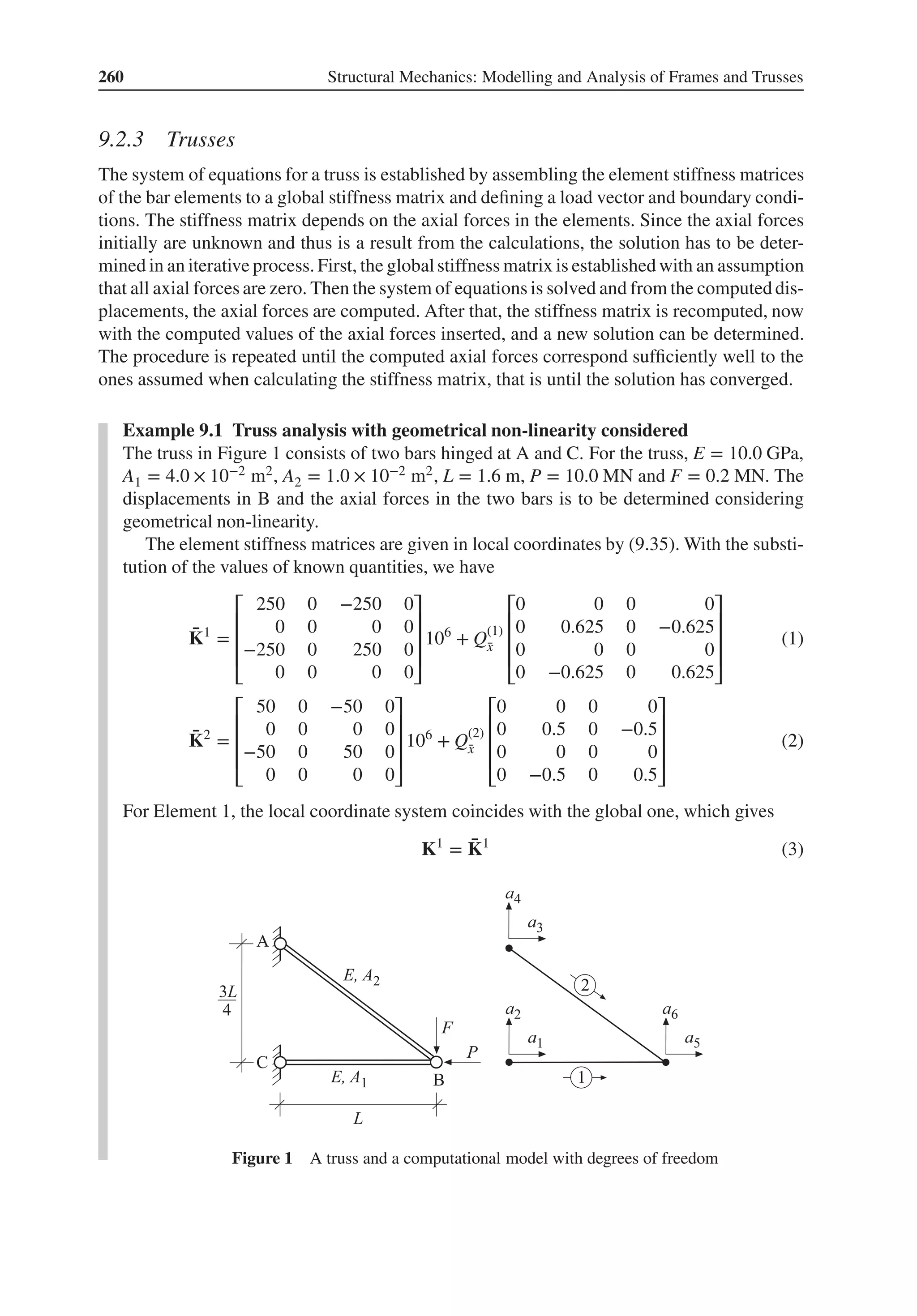
![Geometrical Non-Linearity 261
For Element 2 we have the direction cosines nx̄
x = 0.8, nȳ
x = −0.6, nx̄
y = 0.6 and nȳ
y = 0.8.
Substitution into (9.38) this yields
K2
=
⎡
⎢
⎢
⎢
⎣
32 −24 −32 24
−24 18 24 −18
−32 24 32 −24
24 −18 −24 18
⎤
⎥
⎥
⎥
⎦
106
+ Q(2)
̄
x
⎡
⎢
⎢
⎢
⎣
0.18 0.24 −0.18 −0.24
0.24 0.32 −0.24 −0.32
−0.18 −0.24 0.18 0.24
−0.24 −0.32 0.24 0.32
⎤
⎥
⎥
⎥
⎦
(4)
Assembling the element stiffness matrices gives a global stiffness matrix K and substituting
the loads P and F into the load vector f, we obtain a system of equations Ka = f for the
truss. Taking the boundary conditions a1 = 0, a2 = 0, a3 = 0 and a4 = 0 into consideration,
the system of equations can be reduced to
[
282 × 106 + 0.18Q(2)
̄
x −24 × 106 + 0.24Q(2)
̄
x
−24 × 106 + 0.24Q(2)
̄
x 18 × 106 + 0.625Q(1)
̄
x + 0.32Q(2)
̄
x
]
[
a5
a6
]
=
[
−10 × 106
−0.2 × 10⁶
]
(5)
The stiffness matrix depends on the axial forces Q(1)
̄
x and Q(2)
̄
x , which are unknown at the
beginning of the computation. To obtain a solution, we use an iterative procedure. We start
by solving the system of equations with Q(1)
̄
x = 0 and Q(2)
̄
x = 0, which gives
[
a5
a6
]
=
[
−41.067
−65.867
]
10−3
(6)
Transformation of the computed displacements to local coordinates and substitution into
(9.26) give the axial forces
Q(1)
̄
x = −10.2667 × 10⁶
(7)
Q(2)
̄
x = 0.3333 × 10⁶
(8)
The new values of Q(1)
̄
x and Q(2)
̄
x are substituted into the system of equations, then the dis-
placements and thereafter the axial forces are recomputed. The procedure is repeated until
the axial forces computed in a step correspond sufficiently well to the values used to com-
pute the element stiffness matrices in that step. In this example, the solution has converged
after six iterations; see Table 1.
Table 1 Computed displacements and axial forces
Iteration number a5 (mm) a6 (mm) Q(1)
̄
x (MN) Q(2)
̄
x (MN)
1 −41.067 −65.867 −10.2667 0.3333
2 −44.653 −108.477 −11.1632 1.4682
3 −44.569 −109.106 −11.1421 1.4905
4 −44.544 −108.843 −11.1359 1.4835
5 −44.544 −108.833 −11.1360 1.4833
6 −44.544 −108.835 −11.1360 1.4833
The vertical displacement at B is 1.6 times larger than in the linear computation (itera-
tion 1) and the axial force in Element 2 is 4.5 times larger.](https://image.slidesharecdn.com/structuralmechanicsmodellingandanalysisofframesandtrussespdfdrive-230720064114-5e1f9a93/75/Structural-mechanics-_-modelling-and-analysis-of-frames-and-trusses-PDFDrive-pdf-275-2048.jpg)
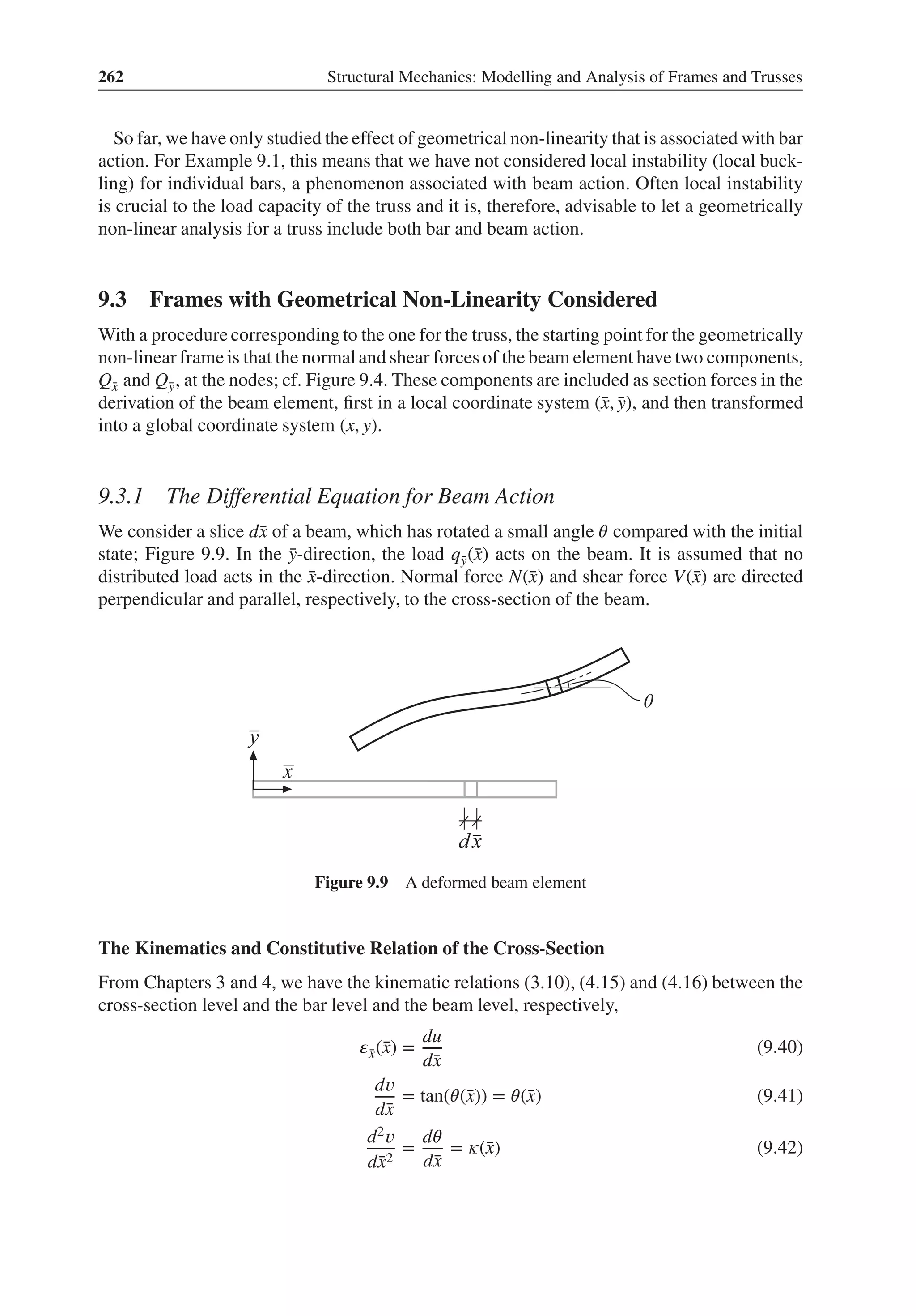
![Geometrical Non-Linearity 263
where u(̄
x), 𝑣(̄
x) and 𝜃(̄
x) are the displacements and rotation of the system line and where 𝜀̄
x
and 𝜅(̄
x) are the strain and curvature, respectively, of the cross-section. Moreover, we have the
constitutive relations (3.16) and (4.12)
N(̄
x) = DEA(̄
x) 𝜀̄
x(̄
x) (9.43)
M(̄
x) = DEI(̄
x) 𝜅(̄
x) (9.44)
between the force measures N(̄
x) and M(̄
x) of the cross-section and its deformation measures
𝜀̄
x(̄
x) and 𝜅̄
x(̄
x).
Equilibrium
At the deformed cross-section, normal force N(̄
x) and shear force V(̄
x) act perpendicular
and parallel, respectively, to the cross-sectional surface. When we establish equilibria in the
deformed state, we use the directions of the coordinates ̄
x and ̄
y, thus we obtain the section
forces in these directions as axial force Q̄
x(̄
x) and transverse force Q̄
y(̄
x) (Figure 9.10). Q̄
x(̄
x)
and Q̄
y(̄
x) can also be expressed in normal force N(̄
x) and shear force V(̄
x)
Q̄
x(̄
x) = N(̄
x) cos 𝜃(̄
x) − V(̄
x) sin 𝜃(̄
x) (9.45)
Q̄
y(̄
x) = N(̄
x) sin 𝜃(̄
x) + V(̄
x) cos 𝜃(̄
x) (9.46)
or [
Q̄
x(̄
x)
Q̄
y(̄
x)
]
=
[
cos 𝜃(̄
x) − sin 𝜃(̄
x)
sin 𝜃(̄
x) cos 𝜃(̄
x)
]
[
N(̄
x)
V(̄
x)
]
(9.47)
Inversely, we have [
N(̄
x)
V(̄
x)
]
=
[
cos 𝜃(̄
x) sin 𝜃(̄
x)
− sin 𝜃(̄
x) cos 𝜃(̄
x)
]
[
Q̄
x(̄
x)
Q̄
y(̄
x)
]
(9.48)
Since the angle 𝜃 is small (sin 𝜃 ≈ tan 𝜃 ≈ 𝜃, cos 𝜃 ≈ 1), the expressions (9.47) and (9.48) can
be written as
[
Q̄
x(̄
x)
Q̄
y(̄
x)
]
=
[
1 −𝜃(̄
x)
𝜃(̄
x) 1
]
[
N(̄
x)
V(̄
x)
]
(9.49)
[
N(̄
x)
V(̄
x)
]
=
[
1 𝜃(̄
x)
−𝜃(̄
x) 1
]
[
Q̄
x(̄
x)
Q̄
y(̄
x)
]
(9.50)
θ
Figure 9.10 Section forces in the deformed cross-section and expressed in the ̄
x̄
y-system](https://image.slidesharecdn.com/structuralmechanicsmodellingandanalysisofframesandtrussespdfdrive-230720064114-5e1f9a93/75/Structural-mechanics-_-modelling-and-analysis-of-frames-and-trusses-PDFDrive-pdf-277-2048.jpg)
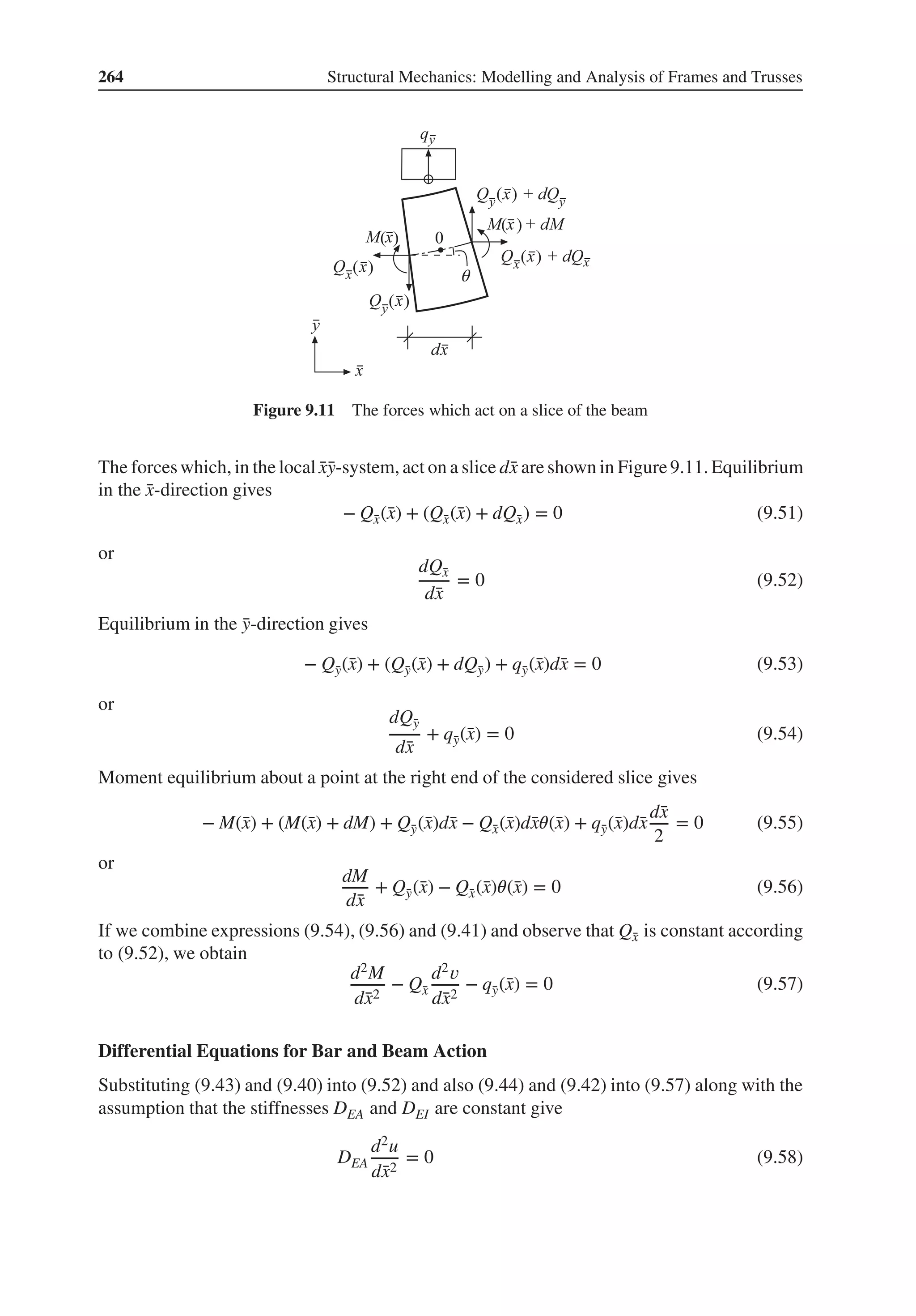
![Geometrical Non-Linearity 265
DEI
d4𝑣
d̄
x4
− Q̄
x
d2𝑣
d̄
x2
− q̄
y(̄
x) = 0 (9.59)
These two differential equations describe bar and beam action with equilibria established in the
deformed state. The expressions show that the axial force Q̄
x locally only affects the bending
stiffness and not the axial stiffness.
9.3.2 Beam Element
For the beam element, we have to introduce six degrees of freedom by which we can express
the components of the normal and shear force of the deformed element.
Solving the Differential Equation for Bar Action
From Chapter 3, we know that the solution to (9.58) can be expressed in terms of the nodal
displacements, here denoted ̄
u1 and ̄
u4 according to Figure 9.12,
u(̄
x) = N̄
ae
=
[
1 − ̄
x
L
̄
x
L
][
̄
u1
̄
u4
]
(9.60)
Then, by substituting (9.40) into (9.43), the normal force can be expressed in terms of nodal
displacements
N = DEA
[
−1
L
1
L
][
̄
u1
̄
u4
]
(9.61)
From (9.50), we have
Q̄
x(̄
x) = N(̄
x) + 𝜃(̄
x)Q̄
y(̄
x) (9.62)
But since a geometrically non-linear analysis is only relevant for large normal forces and since
the kinematics of beam action presume small rotations, the term 𝜃(̄
x)Q̄
y(̄
x) can be neglected,
that is
Q̄
x(̄
x) = N(̄
x) (9.63)
Substitution of (9.61) gives
Q̄
x = DEA
[
−1
L
1
L
][
̄
u1
̄
u4
]
(9.64)
Figure 9.12 A beam element with six degrees of freedom](https://image.slidesharecdn.com/structuralmechanicsmodellingandanalysisofframesandtrussespdfdrive-230720064114-5e1f9a93/75/Structural-mechanics-_-modelling-and-analysis-of-frames-and-trusses-PDFDrive-pdf-279-2048.jpg)
![266 Structural Mechanics: Modelling and Analysis of Frames and Trusses
In Figure 9.12,we have defined the forces that act at the nodesof the element. In the ̄
x-direction,
we have ̄
P1 and ̄
P4 that is
̄
P1 = −Q̄
x(0) (9.65)
̄
P4 = Q̄
x(L) (9.66)
Substituting (9.64), the element relations for bar action can be expressed as
̄
fe
b = ̄
Ke
0
̄
ae
(9.67)
where
̄
Ke
0 =
DEA
L
[
1 −1
−1 1
]
; ̄
ae
=
[
̄
u1
̄
u4
]
; ̄
fe
b =
[
̄
P1
̄
P4
]
(9.68)
Approximate Solution of the Differential Equation for Beam Action
For a beam element, an exact solution can be obtained (see later), but analogous to the solution
for a beam on a transverse flexible support (Chapter 6), we introduce an approximate solution
instead. The differential equation (9.59) can be written as
DEI
d4𝑣
d̄
x4
+ p̄
y(̄
x) − q̄
y(̄
x) = 0 (9.69)
where the effect of the axial force Q̄
x on the beam has been interpreted as an effect of a dis-
tributed load
p̄
y(̄
x) = −Q̄
x
d2𝑣
d̄
x2
(9.70)
If we assume that the transverse displacement varies as a third-degree polynomial, the load
p̄
y(̄
x) in the differential equation can be written as
p̄
y(̄
x) = −Q̄
x
d2N
d̄
x2
̄
ae
(9.71)
where N̄
ae is the third-degree polynomial expressed in terms of the nodal displacements of the
beam, according to (4.47). The homogeneous equation corresponding to (9.69) is
DEI
d4𝑣h
d̄
x4
= 0 (9.72)
As we have seen in Chapter 4, the solution of (9.72) is given from (4.47)
𝑣h(̄
x) = N̄
ae
(9.73)
where according to (4.48) and (4.44)
N = ̄
NC−1
=
[
1 ̄
x ̄
x2 ̄
x3
]
⎡
⎢
⎢
⎢
⎢
⎢
⎢
⎣
1 0 0 0
0 1 0 0
− 3
L2 −2
L
3
L2 −1
L
2
L3
1
L2 − 2
L3
1
L2
⎤
⎥
⎥
⎥
⎥
⎥
⎥
⎦
; ̄
ae
=
⎡
⎢
⎢
⎢
⎢
⎢
⎢
⎣
̄
u2
̄
u3
̄
u5
̄
u6
⎤
⎥
⎥
⎥
⎥
⎥
⎥
⎦
(9.74)](https://image.slidesharecdn.com/structuralmechanicsmodellingandanalysisofframesandtrussespdfdrive-230720064114-5e1f9a93/75/Structural-mechanics-_-modelling-and-analysis-of-frames-and-trusses-PDFDrive-pdf-280-2048.jpg)
![Geometrical Non-Linearity 267
The general solution to (9.69) is
𝑣(̄
x) = 𝑣h(̄
x) + 𝑣p(̄
x) (9.75)
Integrating (9.69) four times with the substitution of (9.71) gives for the case with a constant
load q̄
y
𝑣p(̄
x) =
Q̄
x
DEI
[
0 0 ̄
x4
12
̄
x5
20
]
C−1
̄
ae
+
1
DEI
(
q̄
y
̄
x4
24
+ C1
̄
x3
6
+ C2
̄
x2
2
+ C3 ̄
x + C4
)
(9.76)
The boundary conditions (4.56)–(4.59) give the constants of integration
C1 = −Q̄
x
[
0 0 L 9L2
10
]
C−1
̄
ae
− q̄
y
L
2
(9.77)
C2 = Q̄
x
[
0 0 L2
6
L3
5
]
C−1
̄
ae
+ q̄
y
L2
12
(9.78)
C3 = 0 (9.79)
C4 = 0 (9.80)
Substituting C1, C2, C3 and C4, the particular solution can be written as
𝑣p(̄
x) =
Q̄
x
DEI
[
0 0
(
̄
x4
12
− L̄
x3
6
+ L2 ̄
x2
12
) (
̄
x5
20
− 3L2 ̄
x3
20
+ L3 ̄
x2
10
)]
C−1
̄
ae
+
q̄
y
DEI
(
̄
x4
24
−
L̄
x3
12
+
L2 ̄
x2
24
)
(9.81)
d2𝑣p
d ̄
x2
=
Q̄
x
DEI
[
0 0
(
̄
x2 − L̄
x + L2
6
) (
̄
x3 − 9L2 ̄
x
10
+ L3
5
)]
C−1
̄
ae
+
q̄
y
DEI
(
̄
x2
2
−
L̄
x
2
+
L2
12
)
(9.82)
d3𝑣p
d ̄
x3
=
Q̄
x
DEI
[
0 0 (2̄
x − L)
(
3̄
x2 − 9L2
10
)]
C−1
̄
ae
+
q̄
y
DEI
(
̄
x −
L
2
)
(9.83)
Equation (9.44) together with (9.42) and (9.75) gives an expression for the moment as a func-
tion of ̄
x
M(̄
x) = DEIB̄
ae
+ Mp(̄
x) (9.84)
where
Mp(̄
x) = DEI
d2𝑣p
d̄
x2
(9.85)](https://image.slidesharecdn.com/structuralmechanicsmodellingandanalysisofframesandtrussespdfdrive-230720064114-5e1f9a93/75/Structural-mechanics-_-modelling-and-analysis-of-frames-and-trusses-PDFDrive-pdf-281-2048.jpg)
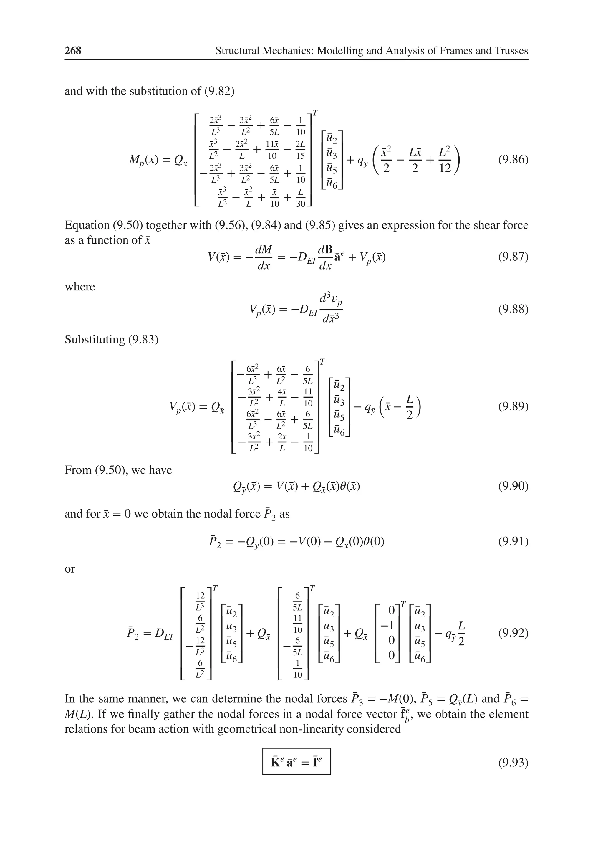
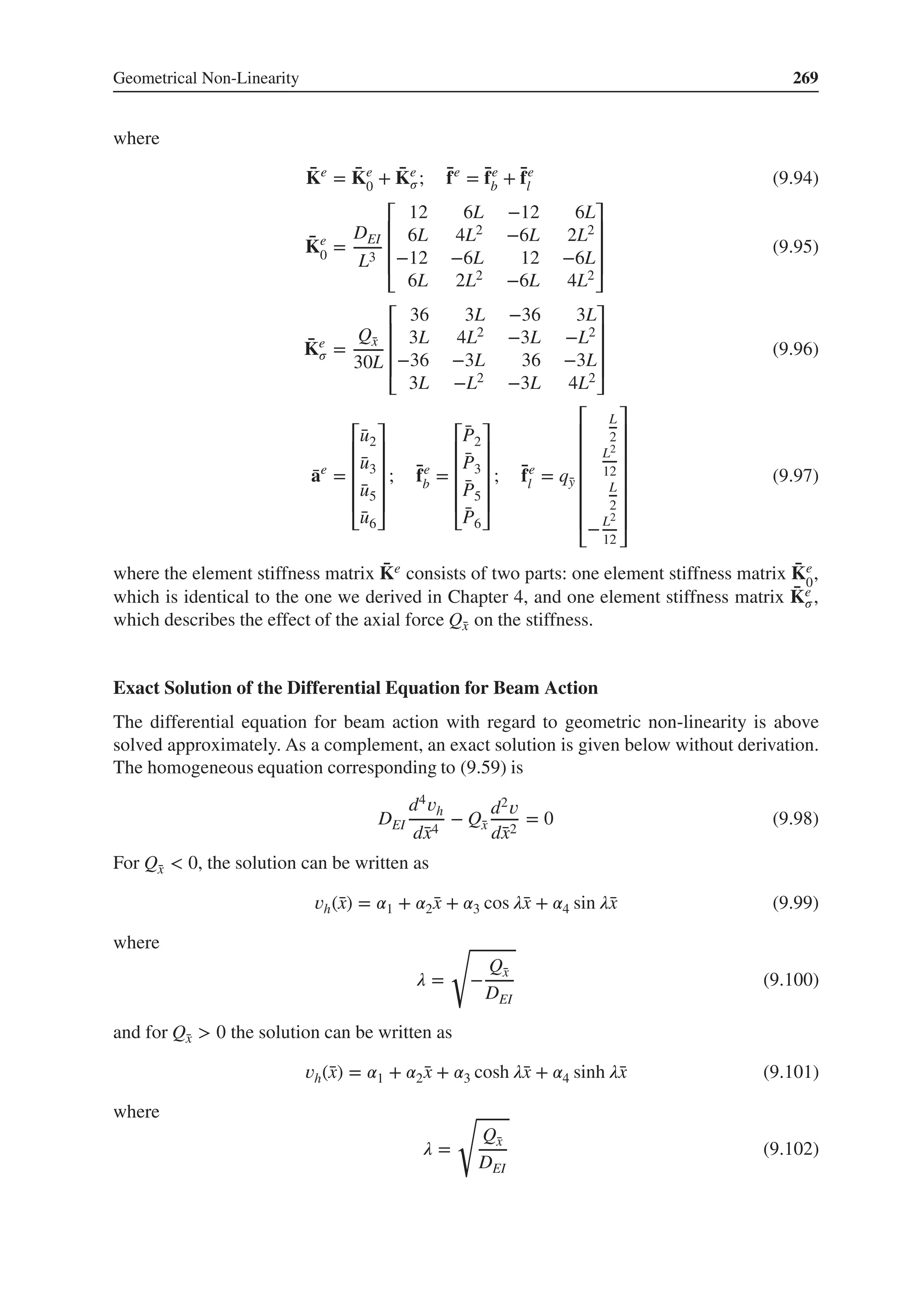
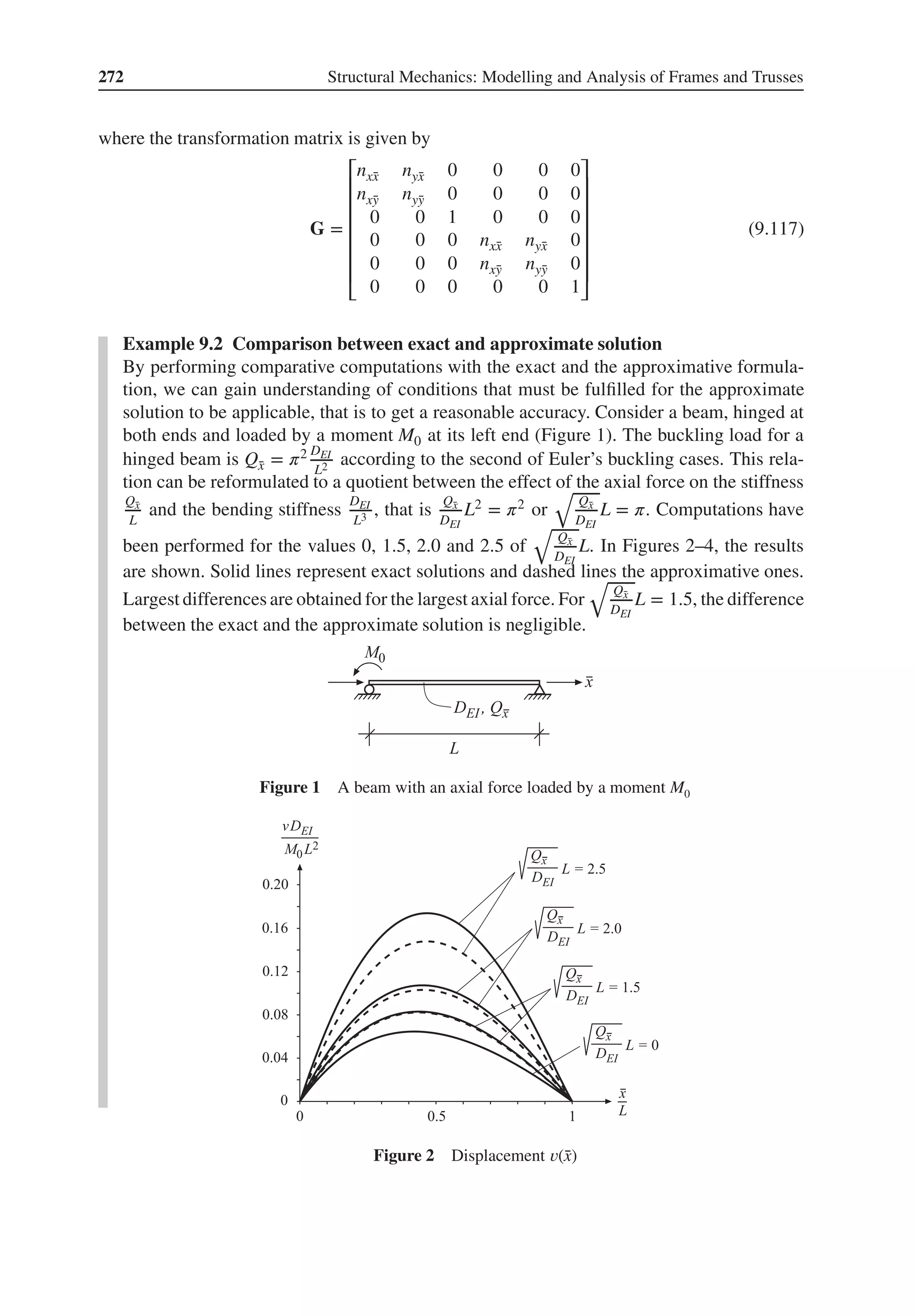
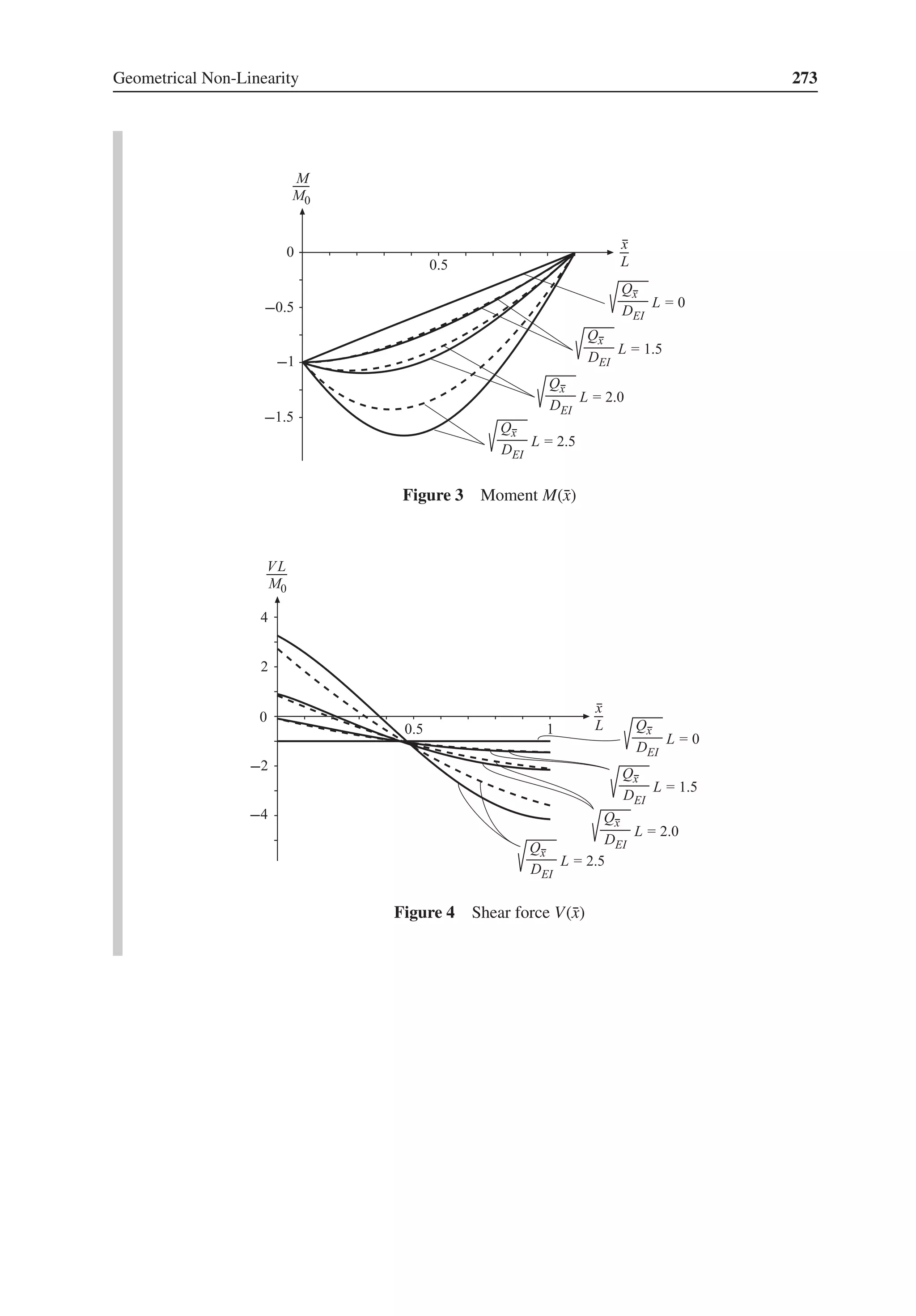
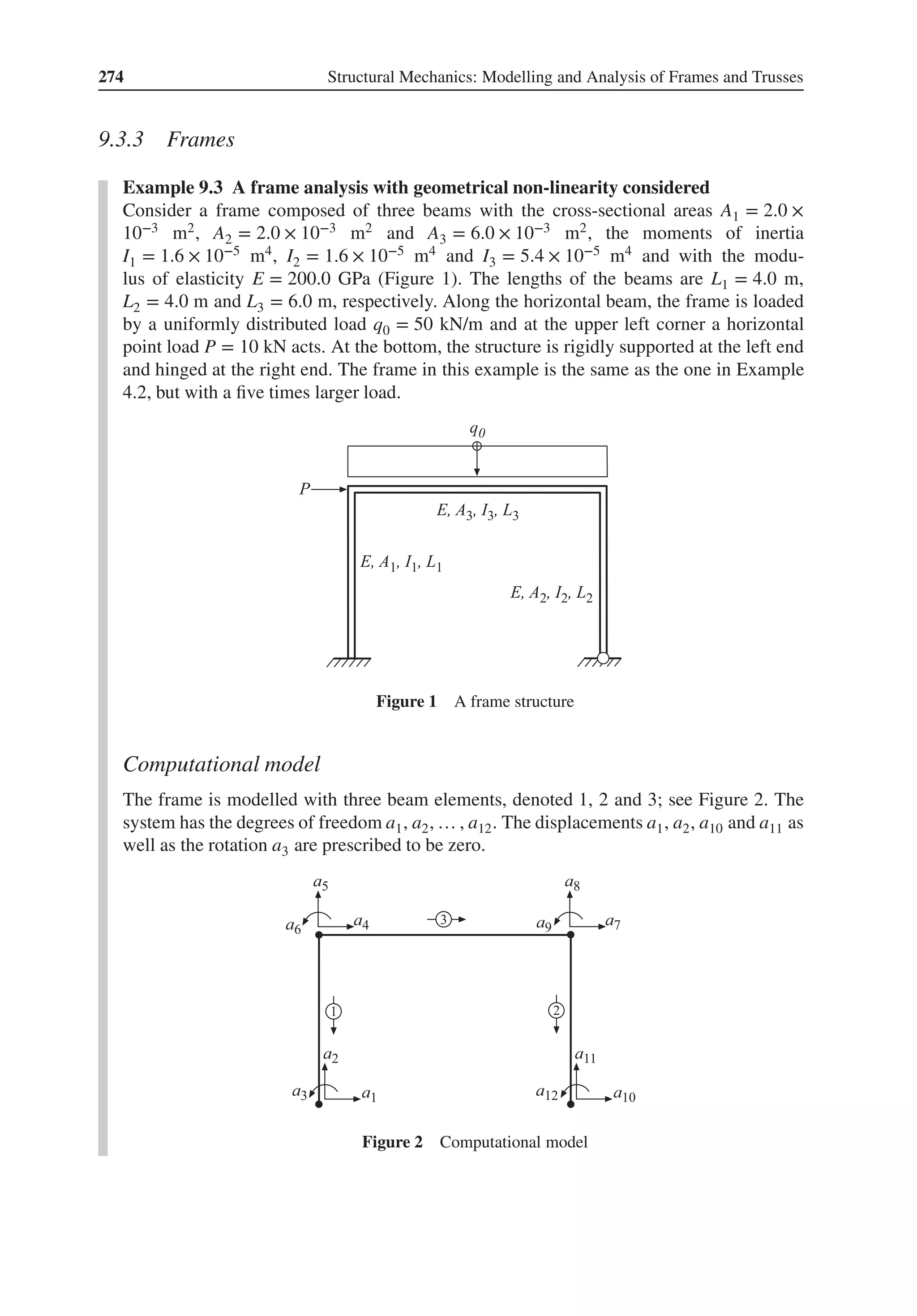
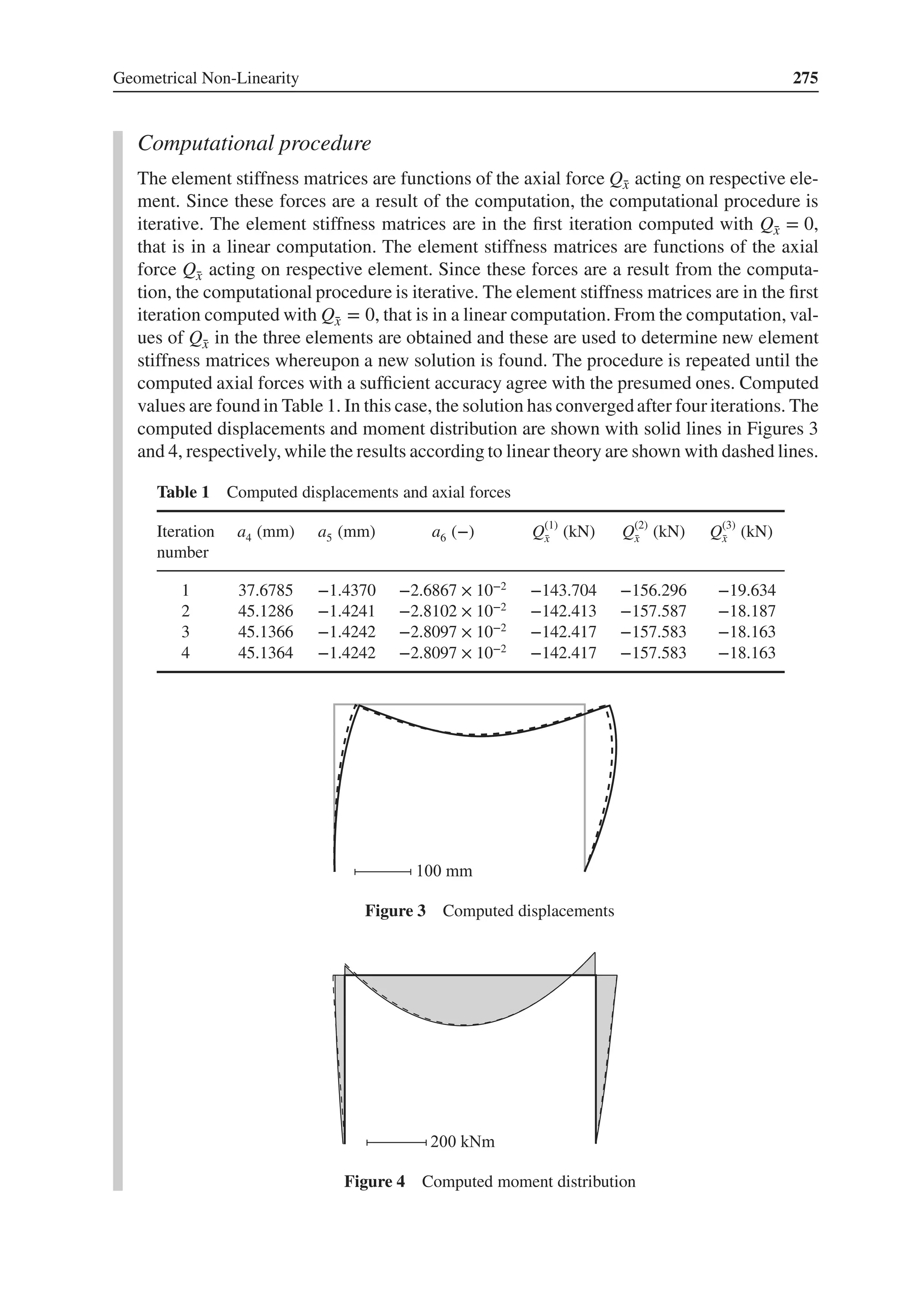
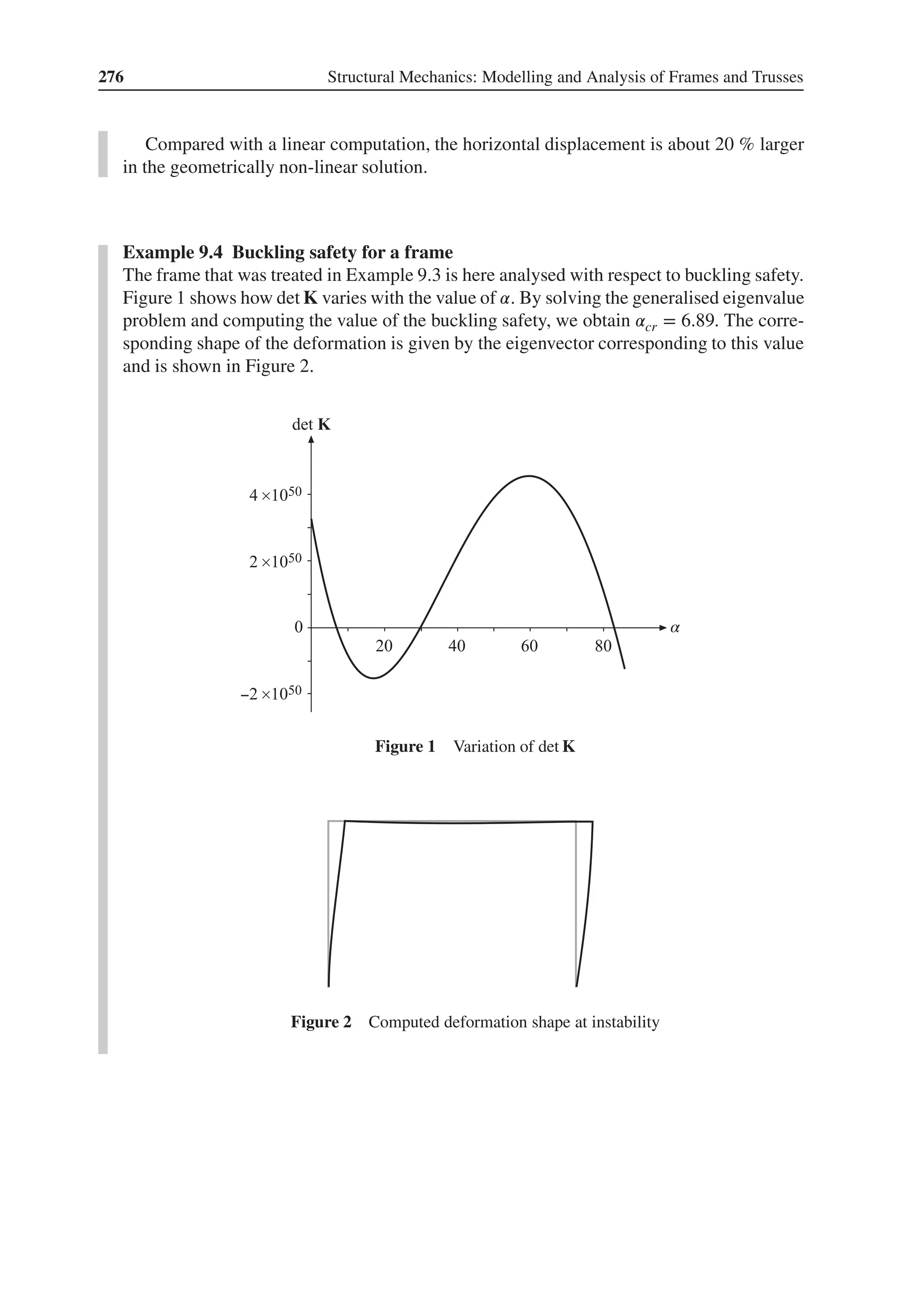
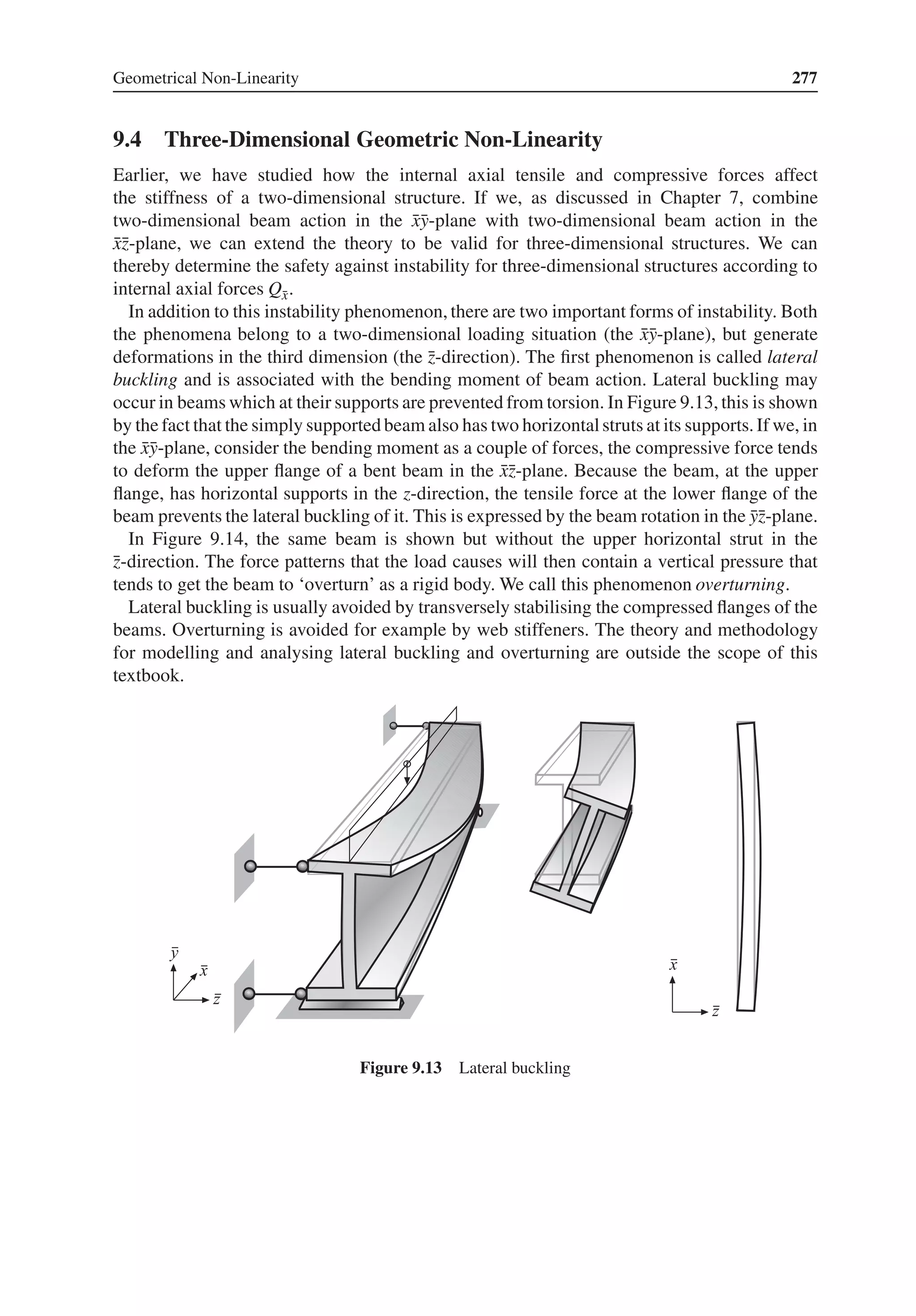
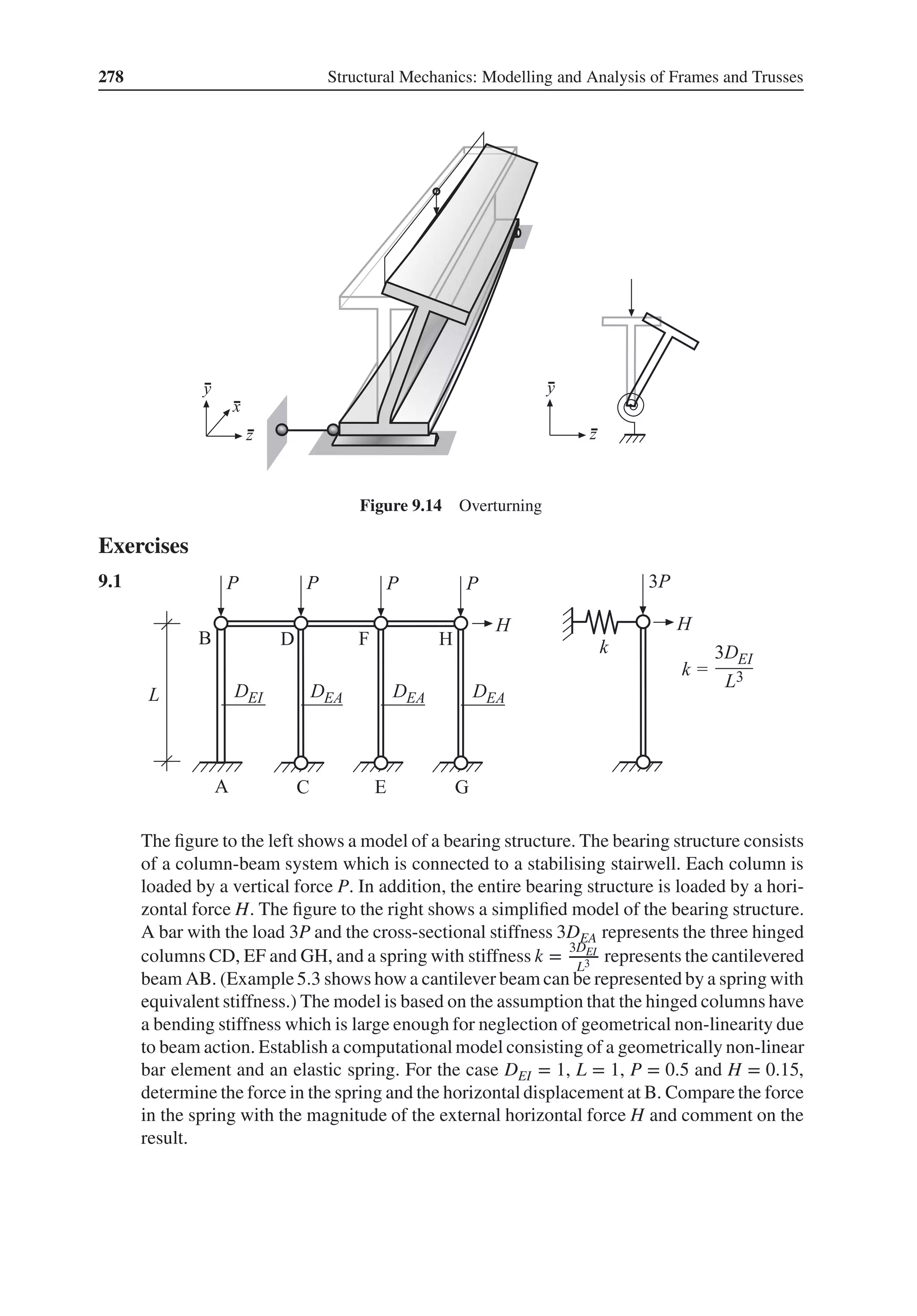
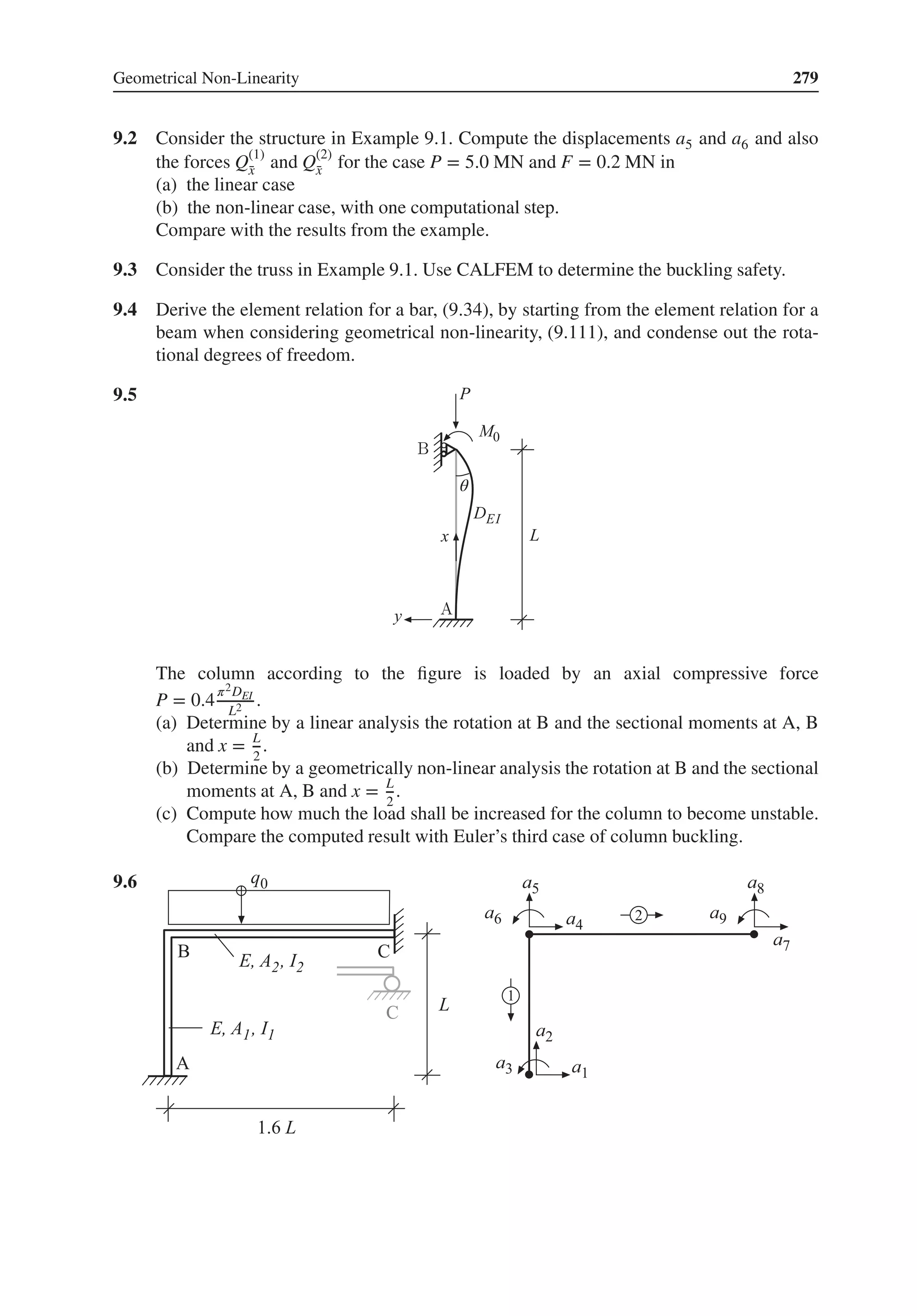
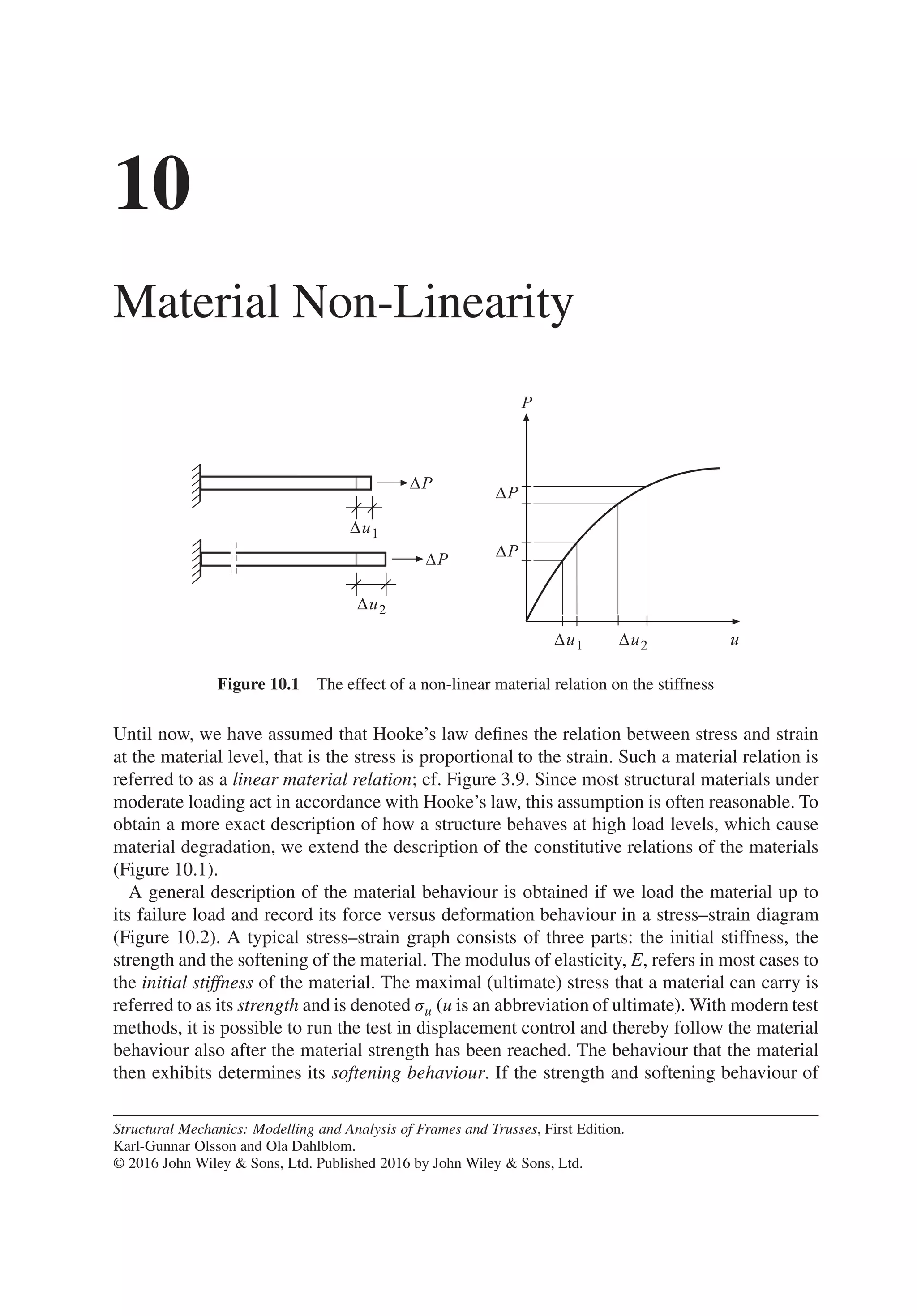
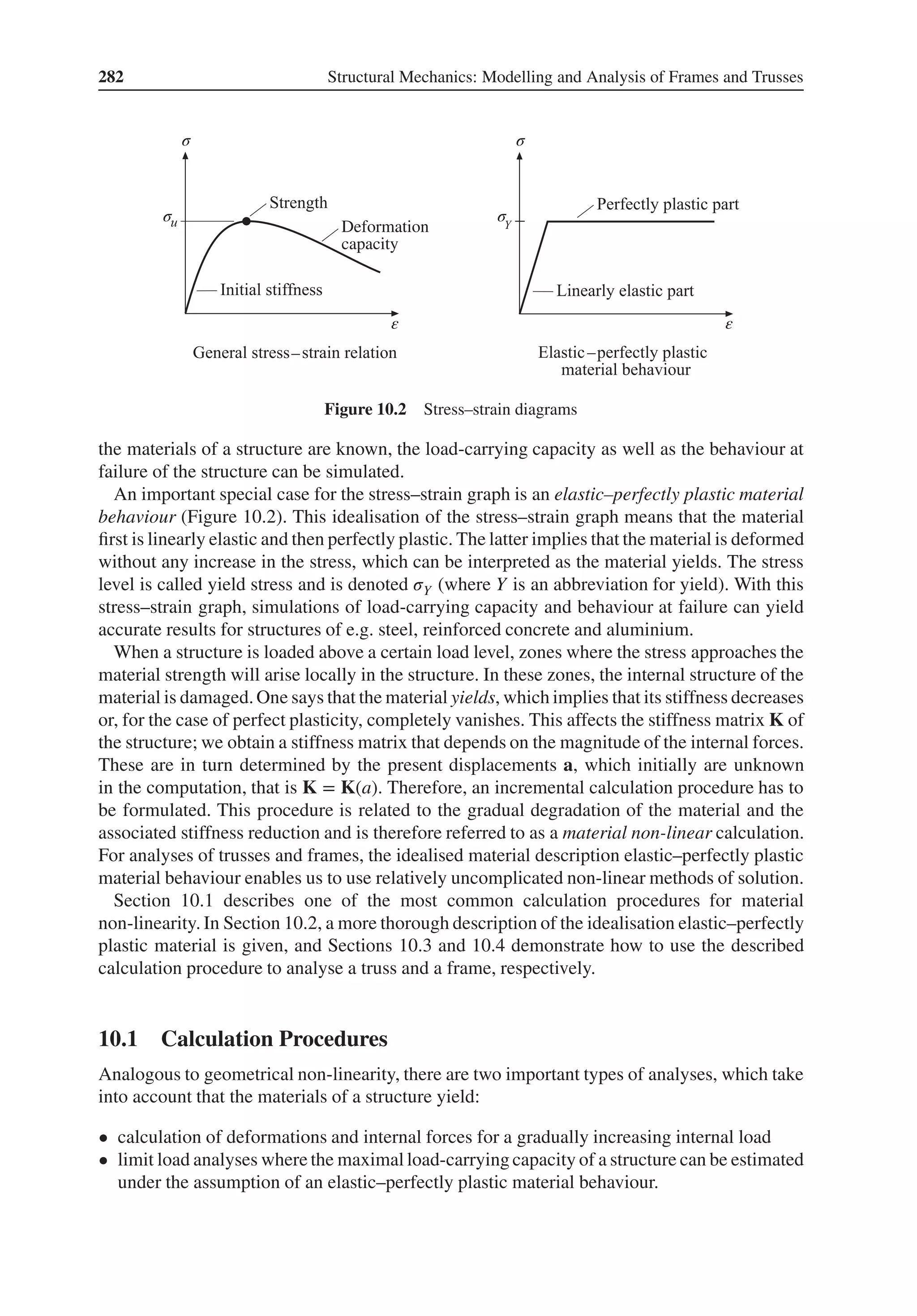
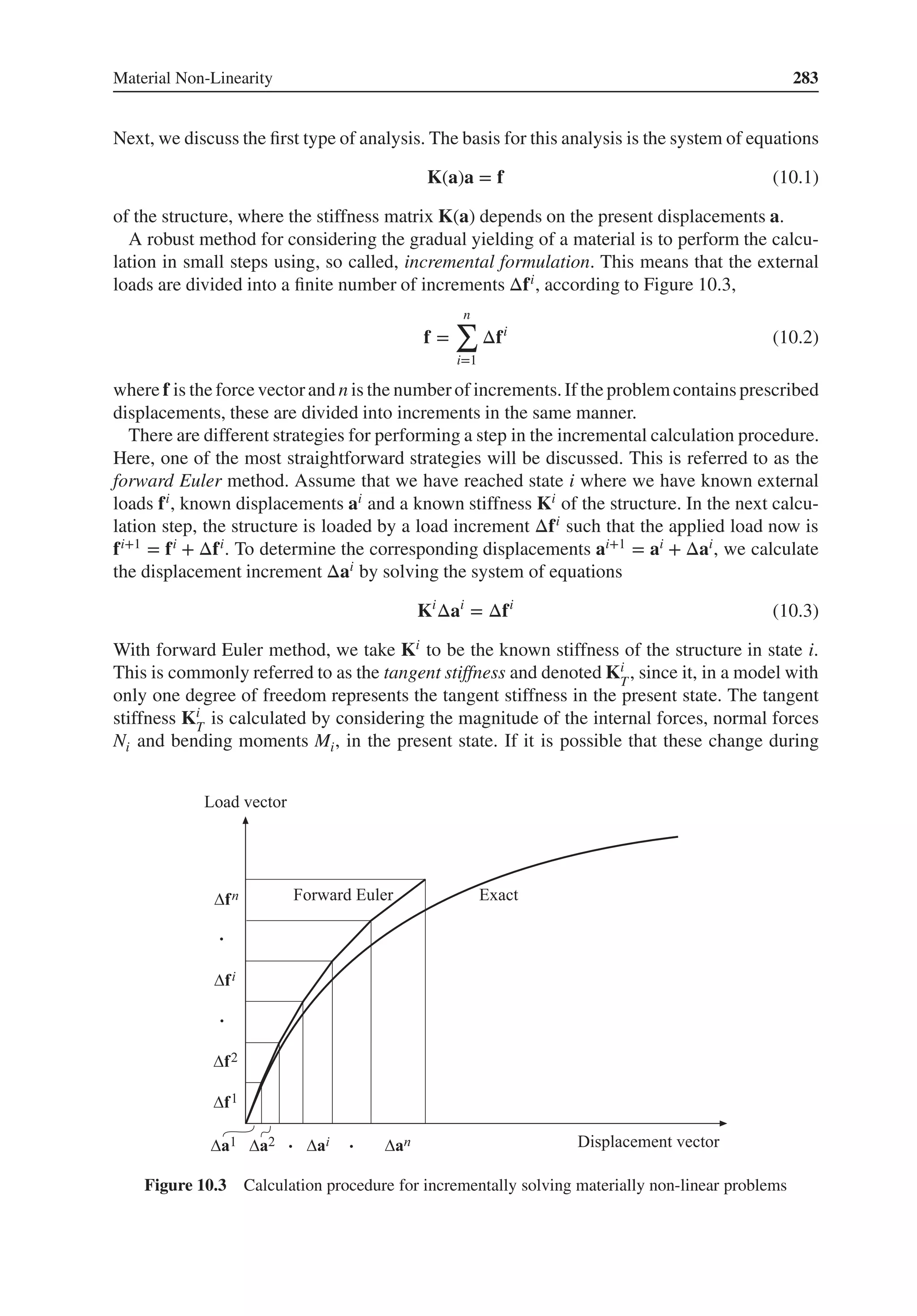
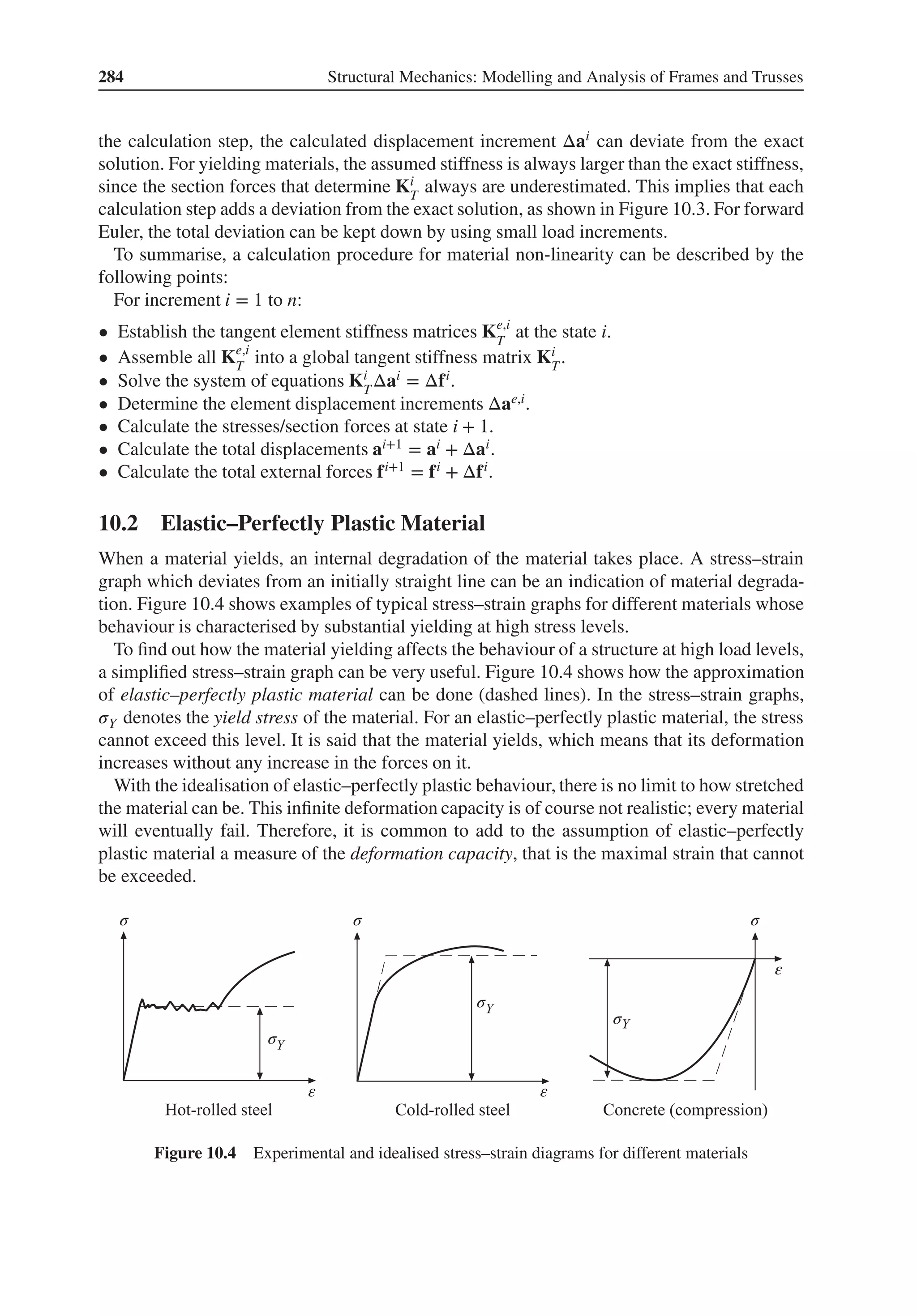
![Material Non-Linearity 285
10.3 Trusses with Material Non-Linearity Considered
The behaviour of a truss at high load levels can be simulated if the model of calculation allows
the material in the bars to yield. Moreover, with such a computational model, the failure load
can be accurately determined. In Section 10.2, it was shown that several of the most common
building materials can be represented by an elastic–perfectly plastic material model. For a
homogeneous cross-section, the stress 𝜎 is constant across the cross-sectional surface of a bar
and the normal force N can according to (3.14) be written as
N =
∫A
𝜎dA = 𝜎A (10.4)
The yield stress 𝜎Y is reached simultaneously across the entire cross-section and correspondsto
a yield force NY = 𝜎YA. For a bar with no externalaxial load and with a constant cross-sectional
area, the stress is the same throughout the entire bar. Thus, yielding will be initiated simulta-
neously in the entire bar.
The calculations become very simple if the analysis of a truss is performed with an
elastic–perfectly plastic material behaviour and by using the forward Euler method. A bar
behaves either elastically or fully plastic. The criterion for when plastic deformations occur
in the bar is N = NY . If N < NY, the bar behaves elastically. There are two different tangent
stiffnesses ET for the material, one for the initial linear-elastic range of action (𝜎 < 𝜎Y)
where ET = E and another one for the plastic range (𝜎 = 𝜎Y) where ET = 0. The incremental
element equation for a bar with elastic–perfectly plastic material can then be written in the
local coordinate system as
ETA
L
[
1 −1
−1 1
]
[
Δu1
Δu2
]
=
[
ΔP1
ΔP2
]
(10.5)
where
ET = E for N < NY
ET = 0 for N = NY (10.6)
How to apply the incremental calculation procedure described in Section 10.1 to the analysis
of a truss by using these relations is shown in Example 10.1.
Example 10.1 Truss analysis with material non-linearity considered
The truss from Example 3.1 is analysed here with an assumption of a non-linear material
behaviour. Each bar is fixed by a hinge in one end and connected to the other bars in a joint
in its other end, as shown in Figure 1. The lengths of the bars are L1 = 1.6 m, L2 = 1.2 m
and L3 =
√
1.62 + 1.22 = 2.0 m, respectively, and the cross-sectional areas are A1 = 6.0 ×
10−4 m2, A2 = 3.0 × 10⁻⁴ m2 and A3 = 10.0 × 10⁻⁴ m2, respectively. The material in the
bars is assumed to be elastic–perfectly plastic with the modulus of elasticity E = 200.0 GPa
and the yield stress 𝜎Y = 400.0 MPa. The truss is loaded by a downwards directed force P
in the free joint and we seek the maximal load Pu that the truss can carry before it becomes
a mechanism due to yielding in the bars and collapses.](https://image.slidesharecdn.com/structuralmechanicsmodellingandanalysisofframesandtrussespdfdrive-230720064114-5e1f9a93/75/Structural-mechanics-_-modelling-and-analysis-of-frames-and-trusses-PDFDrive-pdf-299-2048.jpg)
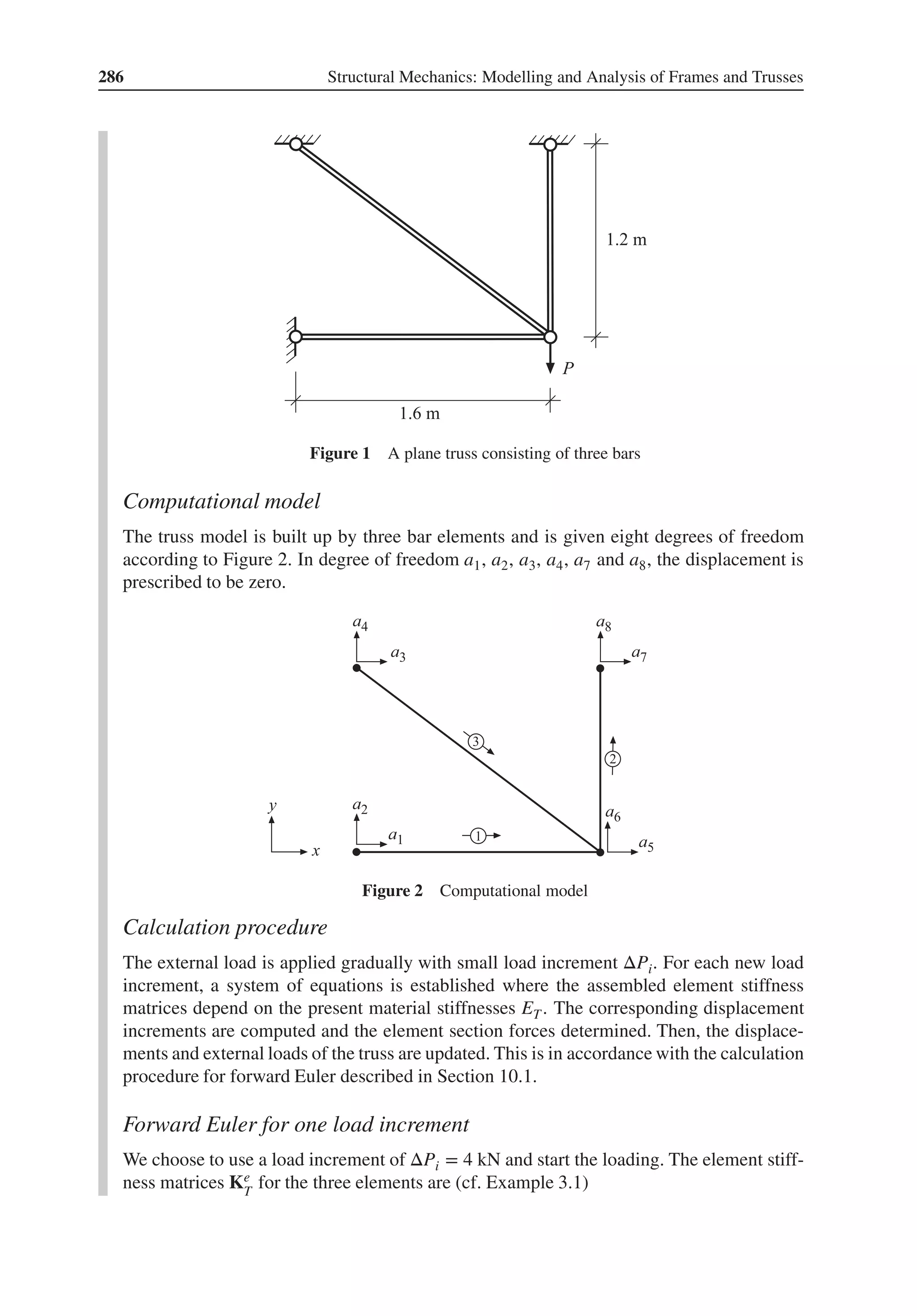
![Material Non-Linearity 287
K1
T =
E(1)
T
⋅ 6.0 × 10−4
1.6
⎡
⎢
⎢
⎢
⎣
1 0 −1 0
0 0 0 0
−1 0 1 0
0 0 0 0
⎤
⎥
⎥
⎥
⎦
(1)
K2
T =
E(2)
T
⋅ 3.0 × 10−4
1.2
⎡
⎢
⎢
⎢
⎣
0 0 0 0
0 1 0 −1
0 0 0 0
0 −1 0 1
⎤
⎥
⎥
⎥
⎦
(2)
K3
T =
E(3)
T
⋅ 10.0 × 10−4
2.0
⎡
⎢
⎢
⎢
⎣
0.64 −0.48 −0.64 0.48
−0.48 0.36 0.48 −0.36
−0.64 0.48 0.64 −0.48
0.48 −0.36 −0.48 0.36
⎤
⎥
⎥
⎥
⎦
(3)
where the modulus of elasticity ET is
ET = 200.0 GPa for N < NY (4)
ET = 0 for N = NY (5)
When the element matrices have been assembled and the system of equations has been
reduced considering prescribed displacements, it becomes
10−5
[
37.5E(1)
T
+ 32E(3)
T
−24E(3)
T
−24E(3)
T
25E(2)
T
+ 18E(3)
T
]
[
Δa5
Δa6
]
=
[
0
−ΔPi
]
103
(6)
which initially, with ET = 200 GPa for all the bars and known quantities inserted, gives
106
[
139 −48
−48 86
][
Δa5
Δa6
]
=
[
0
−4
]
103
(7)
which has the solution [
Δa5
Δa6
]
=
[
−19.90
−57.62
]
10−6
(8)
For Element 1, we have initially the element displacement increments
Δ„
a1
= GΔa1
=
[
1 0 0 0
0 0 1 0
]⎡
⎢
⎢
⎢
⎣
0
0
−19.90
−57.62
⎤
⎥
⎥
⎥
⎦
10−6
=
[
0
−19.90
]
10−6
(9)
which give the normal force increment
ΔN(1)
= EA1BΔ„
a1
= 200.0 × 109
⋅ 6.0 × 10−4 1
1.6
[
−1 1
]
[
0
−19.90
]
10−6
= −1.492 × 10³
(10)](https://image.slidesharecdn.com/structuralmechanicsmodellingandanalysisofframesandtrussespdfdrive-230720064114-5e1f9a93/75/Structural-mechanics-_-modelling-and-analysis-of-frames-and-trusses-PDFDrive-pdf-301-2048.jpg)
![288 Structural Mechanics: Modelling and Analysis of Frames and Trusses
For Elements 2 and 3, we can in the same manner determine the initial values of ΔN(2) and
ΔN(3)
ΔN(2)
= 2.881 × 10³
(11)
ΔN(3)
= 1.865 × 10³
(12)
In the end of each load increment, the element normal forces are updated
Ne,i+1
= Ne,i
+ ΔNe
(13)
as well as the displacements of the truss and the external load
ai+1
= ai
+ Δai
(14)
fi+1
= fi
+ Δfi
(15)
Check for yielding and collapse
To determine the material stiffnesses ET in a new calculation step, the present normal force
N is compared with the yield force NY for each element. The three bar elements have the
yield forces
N(1)
Y
= 𝜎YA1 = 240 kN (16)
N(2)
Y
= 𝜎YA2 = 120 kN (17)
N(3)
Y
= 𝜎YA3 = 400 kN (18)
During the first 41 load increments, none of the normal forces reaches the corresponding
yield force; thus, the initial stiffness matrix
KT = 106
[
139 −48
−48 86
]
(19)
can be used throughout all these increments.
At load increment 42, we obtain N(2),42 = 120.99 kN, which exceeds the yield force of
120 kN. A new and reduced stiffness matrix KT is calculated
KT = 106
[
139 −48
−48 36
]
(20)
where the material stiffness for Element 2 has been reduced to E(2)
T
= 0. Thereafter, we first
check whether the plastic flow in bar Element 2 leads to a collapse of the truss, but since
det KT > 0 there is no collapse yet and we can continue the calculation, where we choose
to keep the load increment ΔPi = 4 kN.
After load increment 76, we obtain N(1),76 = −244.00 kN, which exceeds the yield force
of 240 kN. A new reduced stiffness matrix KT for the truss is calculated
KT = 106
[
64 −48
−48 36
]
(21)
where also the material stiffness E(1)
T
= 0. The determinant of the reduced stiffness matrix
det KT = 0, that is we have a mechanism, the truss has collapsed and the calculation is
terminated.](https://image.slidesharecdn.com/structuralmechanicsmodellingandanalysisofframesandtrussespdfdrive-230720064114-5e1f9a93/75/Structural-mechanics-_-modelling-and-analysis-of-frames-and-trusses-PDFDrive-pdf-302-2048.jpg)
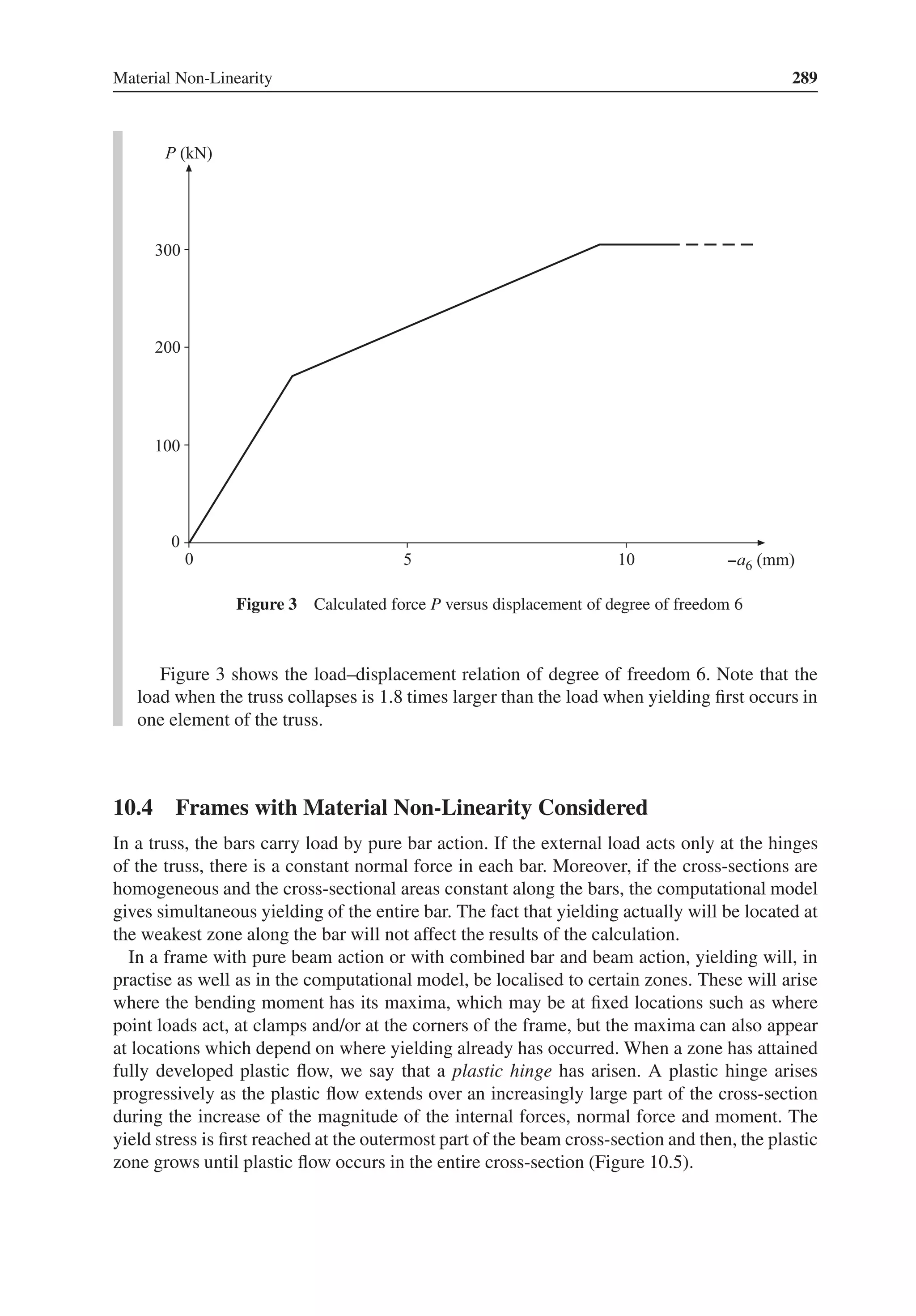
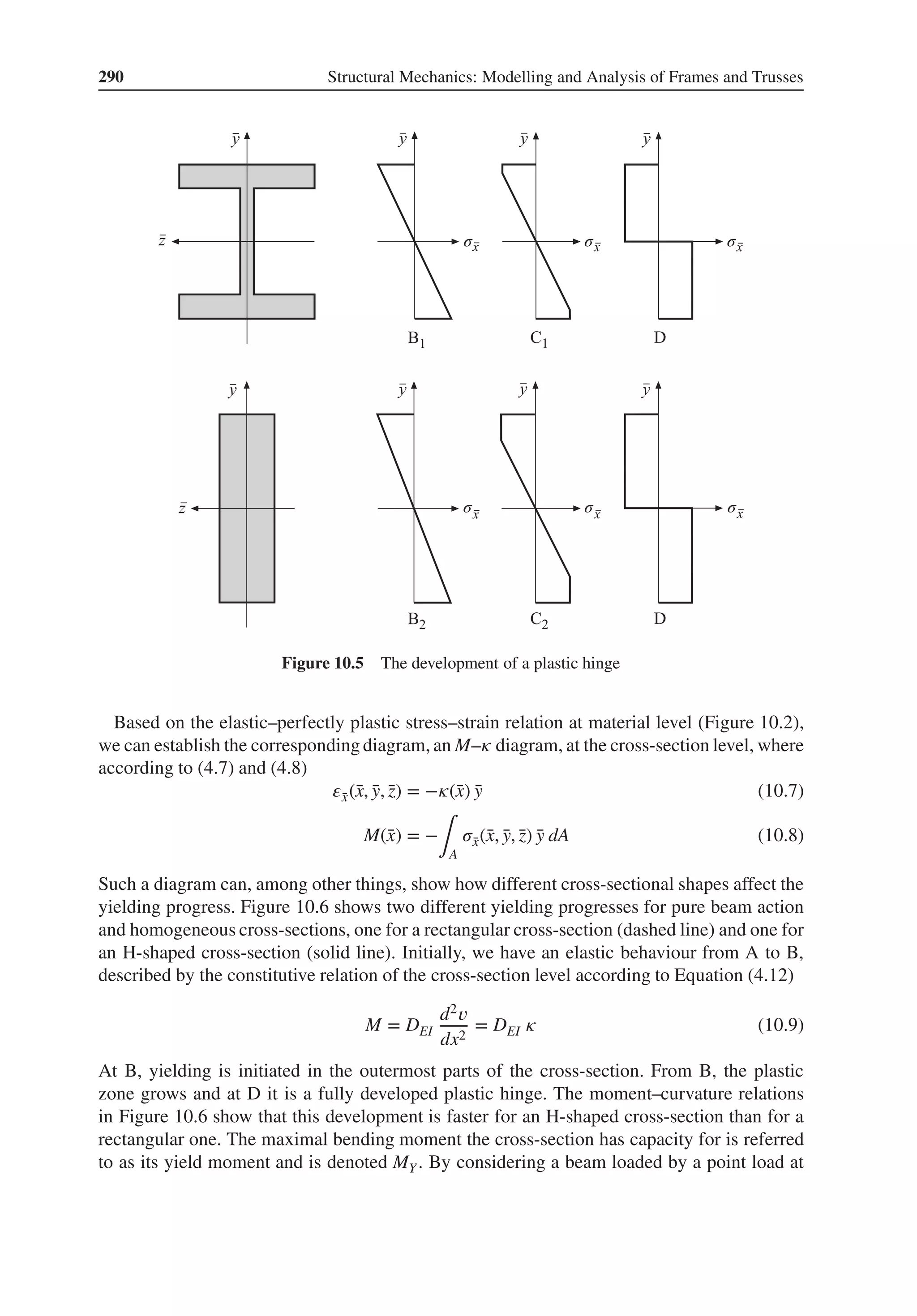
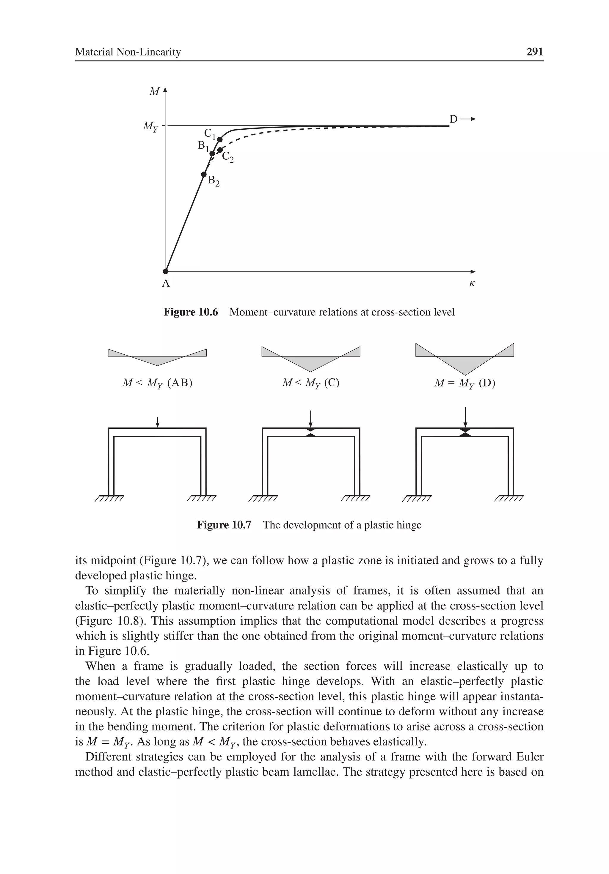
![292 Structural Mechanics: Modelling and Analysis of Frames and Trusses
Figure 10.8 An elastic–perfectly plastic moment–curvature relation at the cross-section level
θ
θ
γ
α
β
Figure 10.9 Modelling of a plastic hinge
that locations where yielding can be expected are predefined in the computational model.
At these locations, a rotational spring is inserted between the adjoining beam elements
(Figure 10.9). A rigid connection between the beam elements can then be modelled by
assigning an infinite stiffness k𝜃 to the inserted springs. In practise, it is appropriate to choose
a k𝜃 that is in an order of magnitude of 104 to 106 times the rotational stiffness of the adjoining
beam elements. This rotational stiffness is
4DEI
L
; cf. K3,3 in (4.87). When yielding occurs, the
plastic hinge is modelled by letting the stiffness of the corresponding rotational spring be
zero, k𝜃 = 0.
Analogous to the bar in a truss, (10.5) and (10.6), an incremental element relation for a
rotational spring can be established.
k𝜃
[
1 −1
−1 1
][
Δu1
Δu2
]
=
[
ΔP1
ΔP2
]
(10.10)
where
k𝜃 = 106
⋅
4DEI
L
for M < MY
k𝜃 = 0 for M = MY (10.11)](https://image.slidesharecdn.com/structuralmechanicsmodellingandanalysisofframesandtrussespdfdrive-230720064114-5e1f9a93/75/Structural-mechanics-_-modelling-and-analysis-of-frames-and-trusses-PDFDrive-pdf-306-2048.jpg)
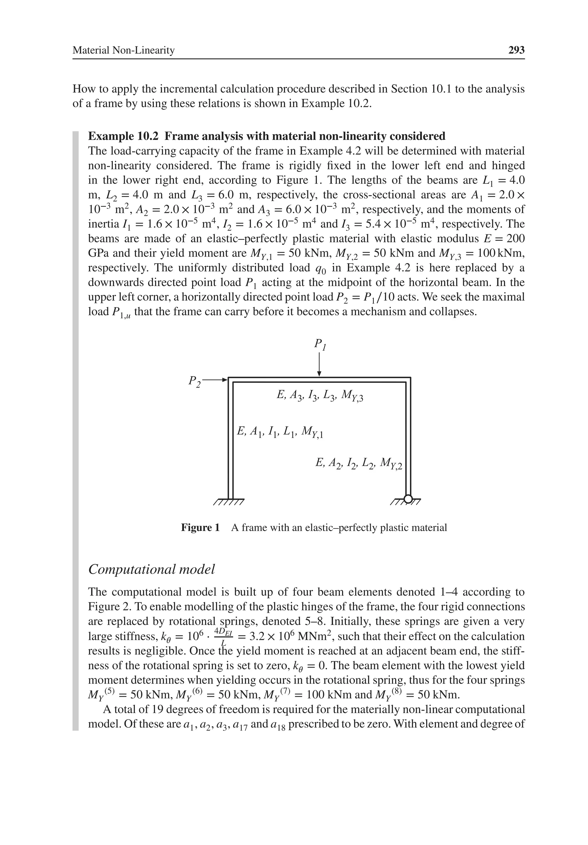
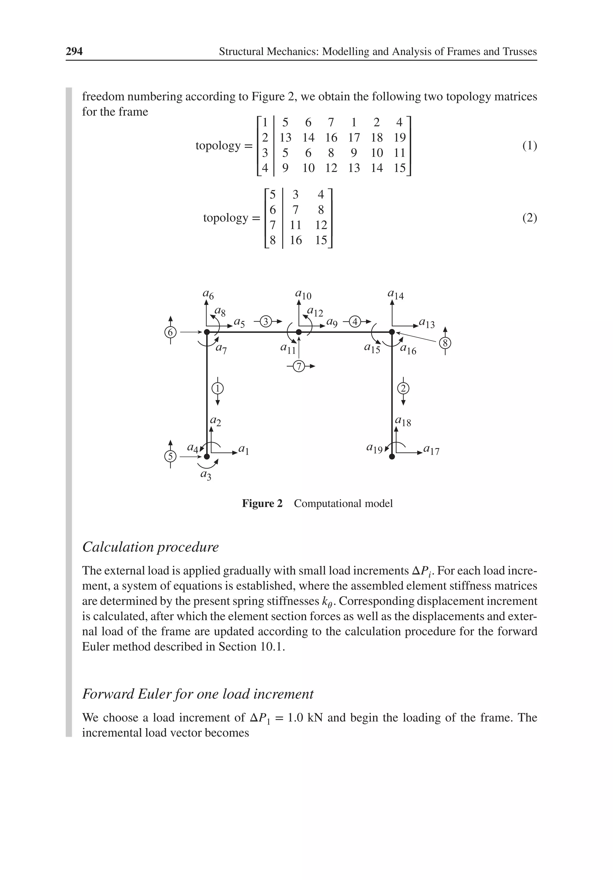
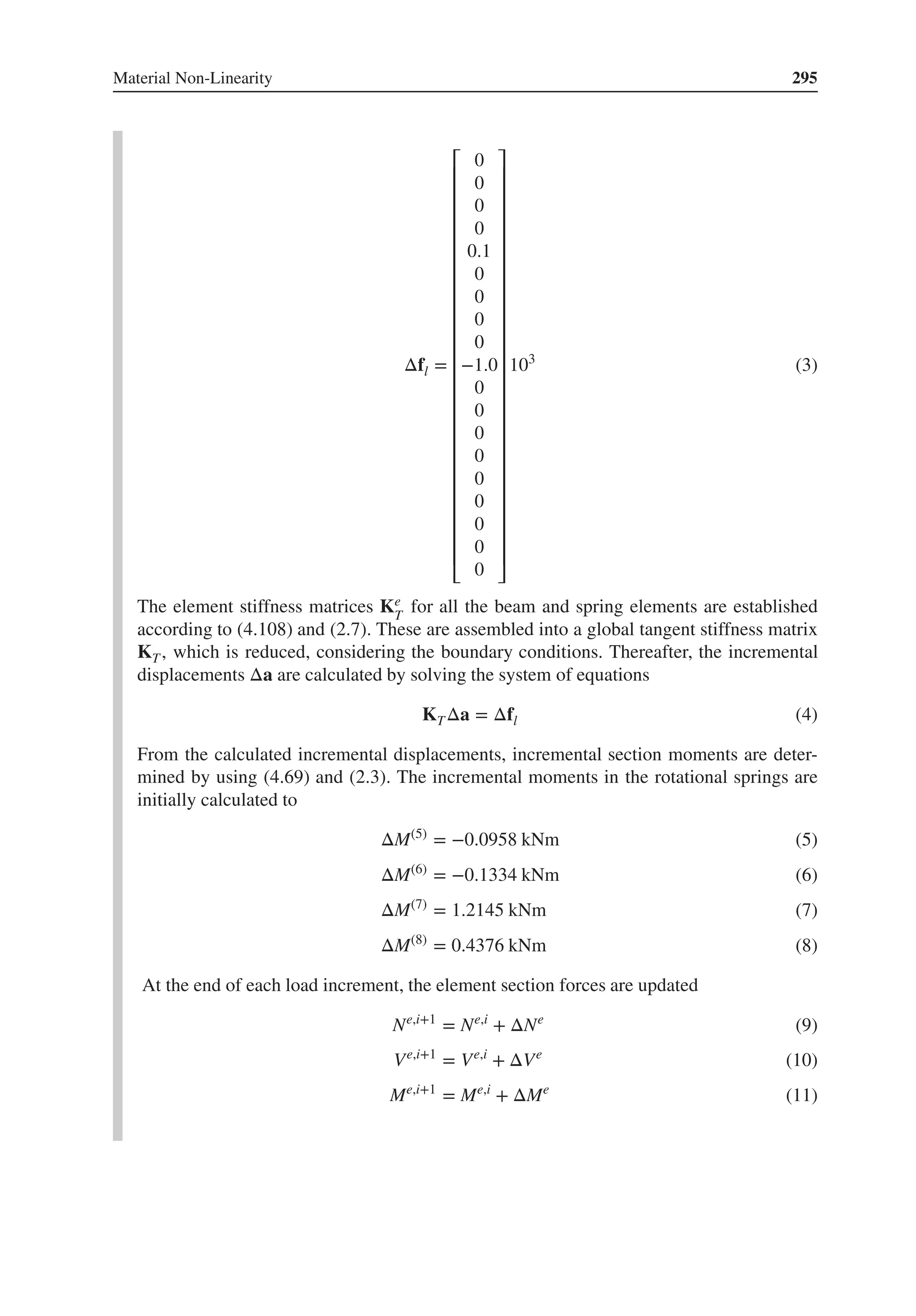
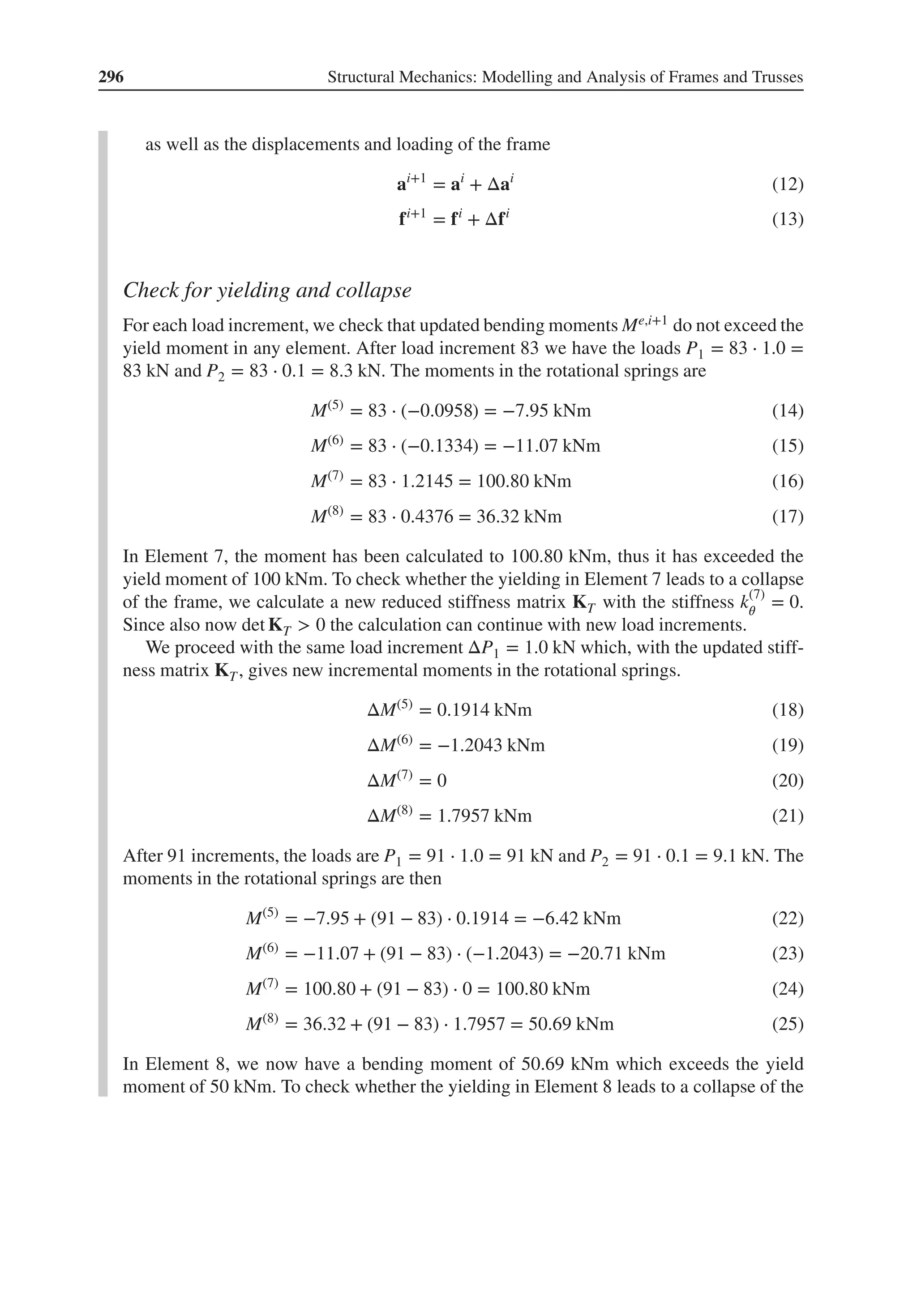
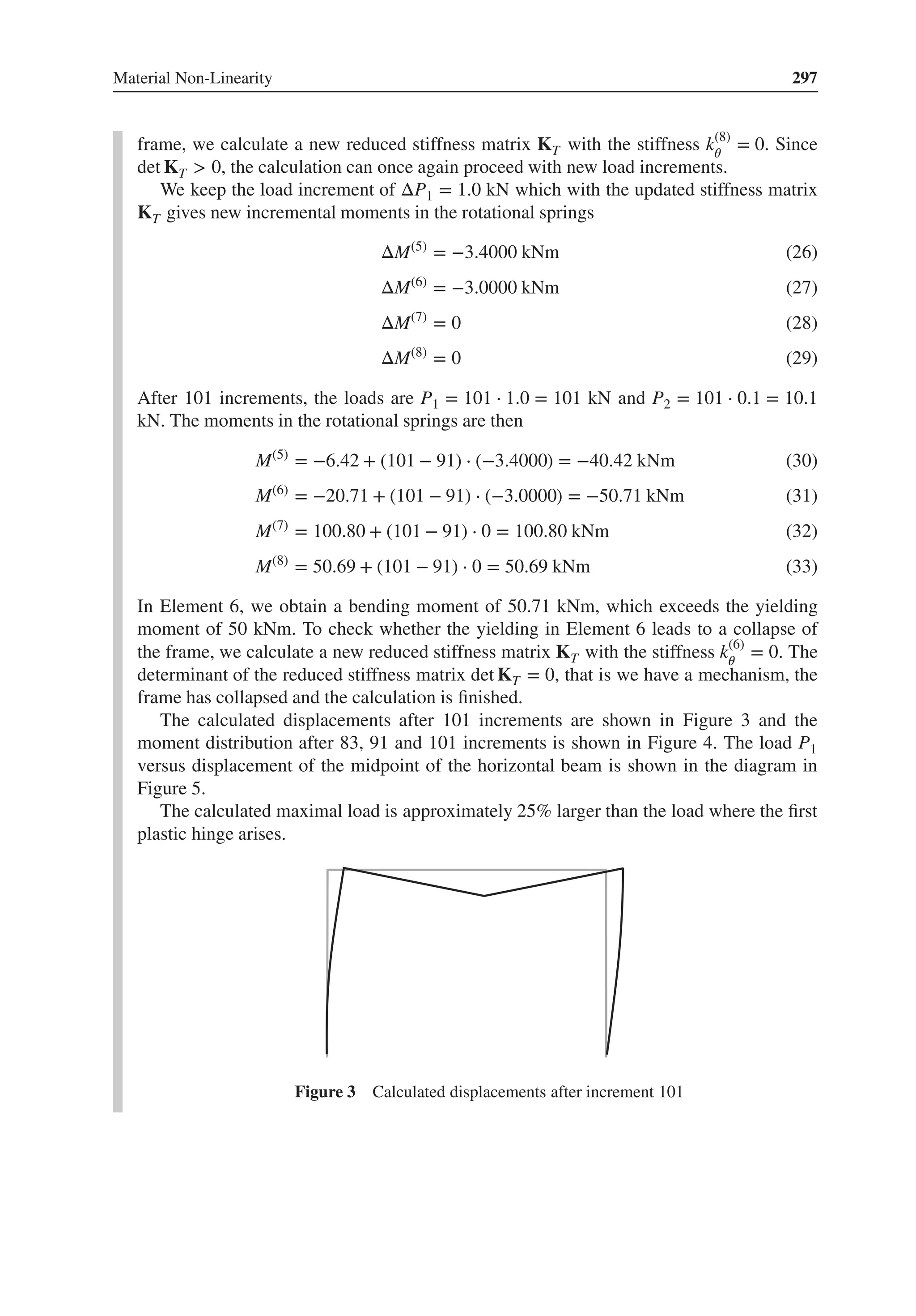
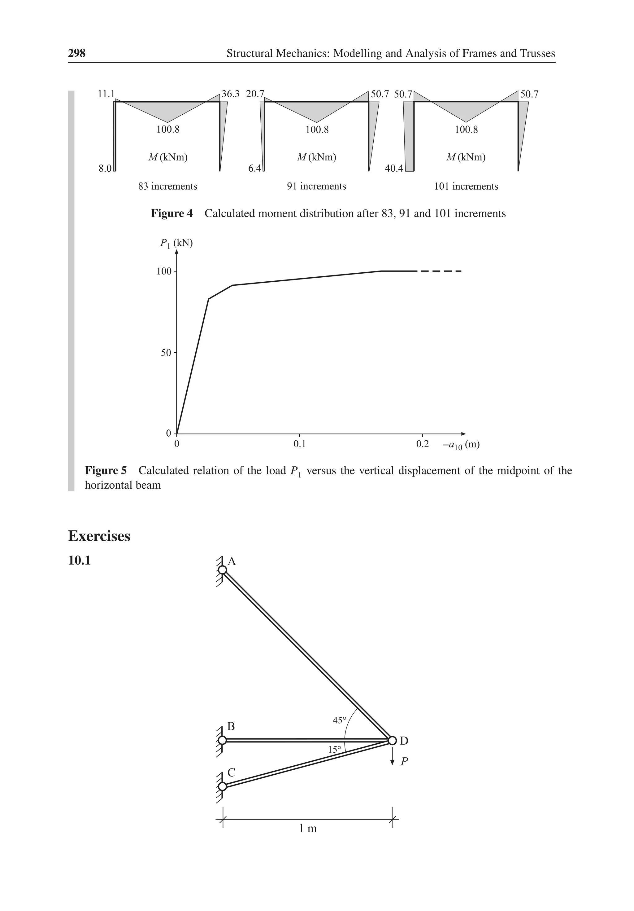
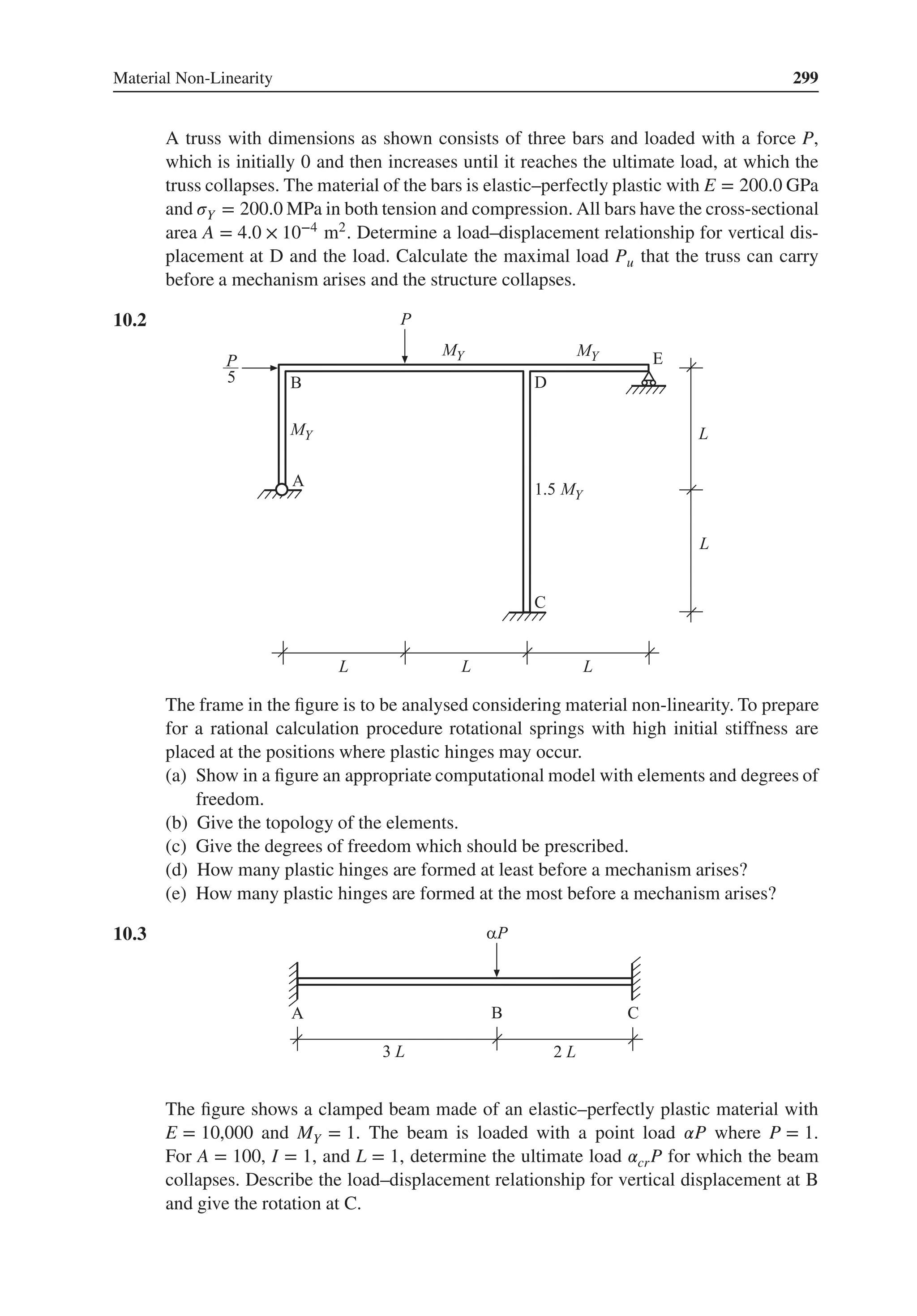
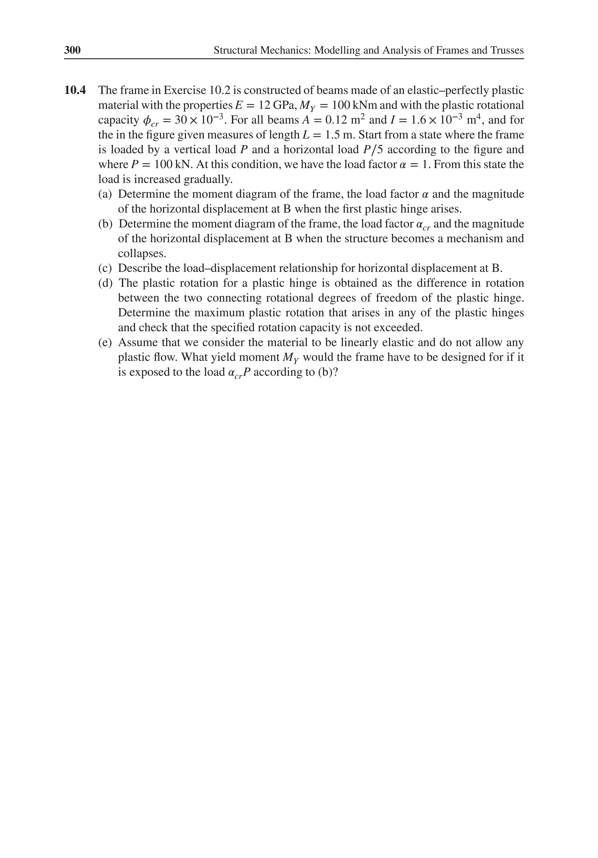
![Appendix B
Answers to the Exercises
1.1 .
(a)
[
2 1 3
5 8 2
]
(b)
[
−10 0
−16 4
]
(c) ⎡
⎢
⎢
⎣
4 8 0
−4 −6 2
16 28 −4
⎤
⎥
⎥
⎦
(d)
[
11 2 8
36 16 20
]
(e) 28
1.2 .
(a) 4 × 6
(b) 3 × 1
(c) it is not possible to perform this operation
(d) 4 × 8
(e) 6 × 4
1.3 ⎡
⎢
⎢
⎣
a1
a2
a3
⎤
⎥
⎥
⎦
=
⎡
⎢
⎢
⎣
1
−2
2
⎤
⎥
⎥
⎦
1.4 .
(a) a3 = 2, f1 = −4, f2 = −6
(b) a2 = 3, a3 = 2, f1 = −10
(c) a2 = −1, a4 = 1, f1 = −8, f3 = −1, f5 = 6
1.5 .
(a) A + B = B + A
(b) AB ≠ BA
Structural Mechanics: Modelling and Analysis of Frames and Trusses, First Edition.
Karl-Gunnar Olsson and Ola Dahlblom.
© 2016 John Wiley & Sons, Ltd. Published 2016 by John Wiley & Sons, Ltd.](https://image.slidesharecdn.com/structuralmechanicsmodellingandanalysisofframesandtrussespdfdrive-230720064114-5e1f9a93/75/Structural-mechanics-_-modelling-and-analysis-of-frames-and-trusses-PDFDrive-pdf-317-2048.jpg)
![304 Appendix B: Answers to the Exercises
(c) (AB)T = BTAT , (BA)T ≠ BT AT
(d) CD 4 × 4-matrix, DC 1 × 1-matrix
(e) CTAC 1 × 1-matrix
(f) det A = 416, AA−1 = I
1.6 .
(a) ⎡
⎢
⎢
⎢
⎣
a1
a2
a3
a4
⎤
⎥
⎥
⎥
⎦
=
⎡
⎢
⎢
⎢
⎣
4
6
1
−4
⎤
⎥
⎥
⎥
⎦
(b) infinitely many solutions, det K = 𝟎, f = 𝟎
(c) there is no unique solution, det K = 𝟎, f ≠ 𝟎
1.7 .
(a) 𝜆1 = 1, 𝜆2 = 11
(b)
a1 = t1
[
1
3
]
, a2 = t2
[
3
−1
]
2.1 a2 = 0.4F
k
, a3 = 0.6F
k
, f1 = −0.4F, f4 = −0.6F, N(1) = 0.4F, N(2) = 0.4F,
N(3) = −0.6F
2.2 a2 = 0.4, a3 = 0.6, f1 = −0.4, f4 = −0.6, N(1) = 0.4, N(2) = 0.4, N(3) = −0.6
2.3 .
(a)
K1 =
[
3 −3
−3 3
]
; K2 =
[
6 −6
−6 6
]
; K3 =
[
7 −7
−7 7
]
; topology =
⎡
⎢
⎢
⎣
1 1 2
2 2 3
3 3 4
⎤
⎥
⎥
⎦
;
K =
⎡
⎢
⎢
⎢
⎣
3 −3 0 0
−3 9 −6 0
0 −6 13 −7
0 0 −7 7
⎤
⎥
⎥
⎥
⎦
(b) det K = 0, there is no unique solution. Boundary conditions not defined, rigid
body motion is not prevented
(c) one
(d) a2 = 0.1543, a3 = 0.1481, f1 = −0.4630, f4 = −1.0370
(e) a2 = 0.0356, a3 = 0.0433, f1 = −0.0467, f4 = 0.0467
2.4
topology =
⎡
⎢
⎢
⎢
⎢
⎢
⎢
⎣
1 1 2
2 2 3
3 3 4
4 3 4
5 2 4
6 4 5
⎤
⎥
⎥
⎥
⎥
⎥
⎥
⎦
K =
⎡
⎢
⎢
⎢
⎢
⎣
k1 −k1 0 0 0
−k1 k1 + k2 + k5 −k2 −k5 0
0 −k2 k2 + k3 + k4 −k3 − k4 0
0 −k5 −k3 − k4 k3 + k4 + k5 + k6 −k6
0 0 0 −k6 k6
⎤
⎥
⎥
⎥
⎥
⎦](https://image.slidesharecdn.com/structuralmechanicsmodellingandanalysisofframesandtrussespdfdrive-230720064114-5e1f9a93/75/Structural-mechanics-_-modelling-and-analysis-of-frames-and-trusses-PDFDrive-pdf-318-2048.jpg)
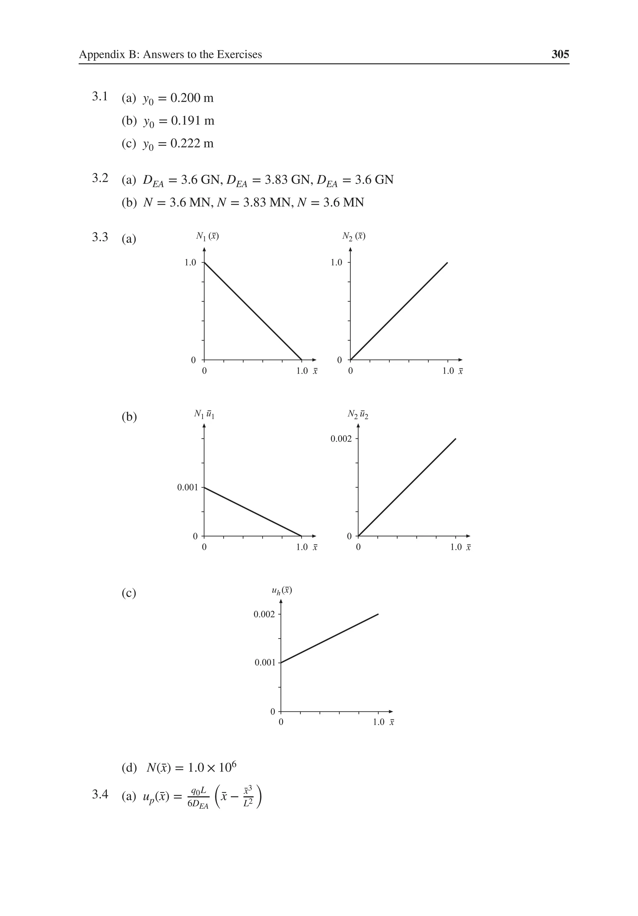
![306 Appendix B: Answers to the Exercises
(b) .
(c) Np(̄
x) =
q0L
6
(
1 − 3̄
x2
L2
)
0.2
–0.2
–0.4
(d) ̄
fe
l
=
q0L
6
[
1
2
]
3.5 uB =
q0L2
3DEA
3.6 u(̄
x) = 7.5 × 10⁻⁴̄
x − 6.25 × 10⁻⁵̄
x3, N(̄
x) = 3.0 × 10⁵ − 7.5 × 10⁴̄
x2
3.7 .
(a) nx̄
x =
√
3
2
= 0.866, nȳ
x = 0.5
(b) nx̄
x = 1
√
10
= 0.316, nȳ
x = 3
√
10
= 0.948
(c) nx̄
x = − 1
√
10
= −0.316, nȳ
x = 3
√
10
= 0.948
3.8
G =
[
0.894 0.447 0 0
0 0 0.894 0.447
]
3.9 Ke
11
: K7,7, Ke
24
: K8,16, Ke
32
: K15,8
3.10 .
(a) ̄
u(7)
1
= −4.128 mm, ̄
u(7)
2
= −5.628 mm
(b) 𝛿 = −1.500 mm, N = −120 kN, 𝜎 = −120 MPa
Note that the displacements have been drawn in exaggerated scale.](https://image.slidesharecdn.com/structuralmechanicsmodellingandanalysisofframesandtrussespdfdrive-230720064114-5e1f9a93/75/Structural-mechanics-_-modelling-and-analysis-of-frames-and-trusses-PDFDrive-pdf-320-2048.jpg)
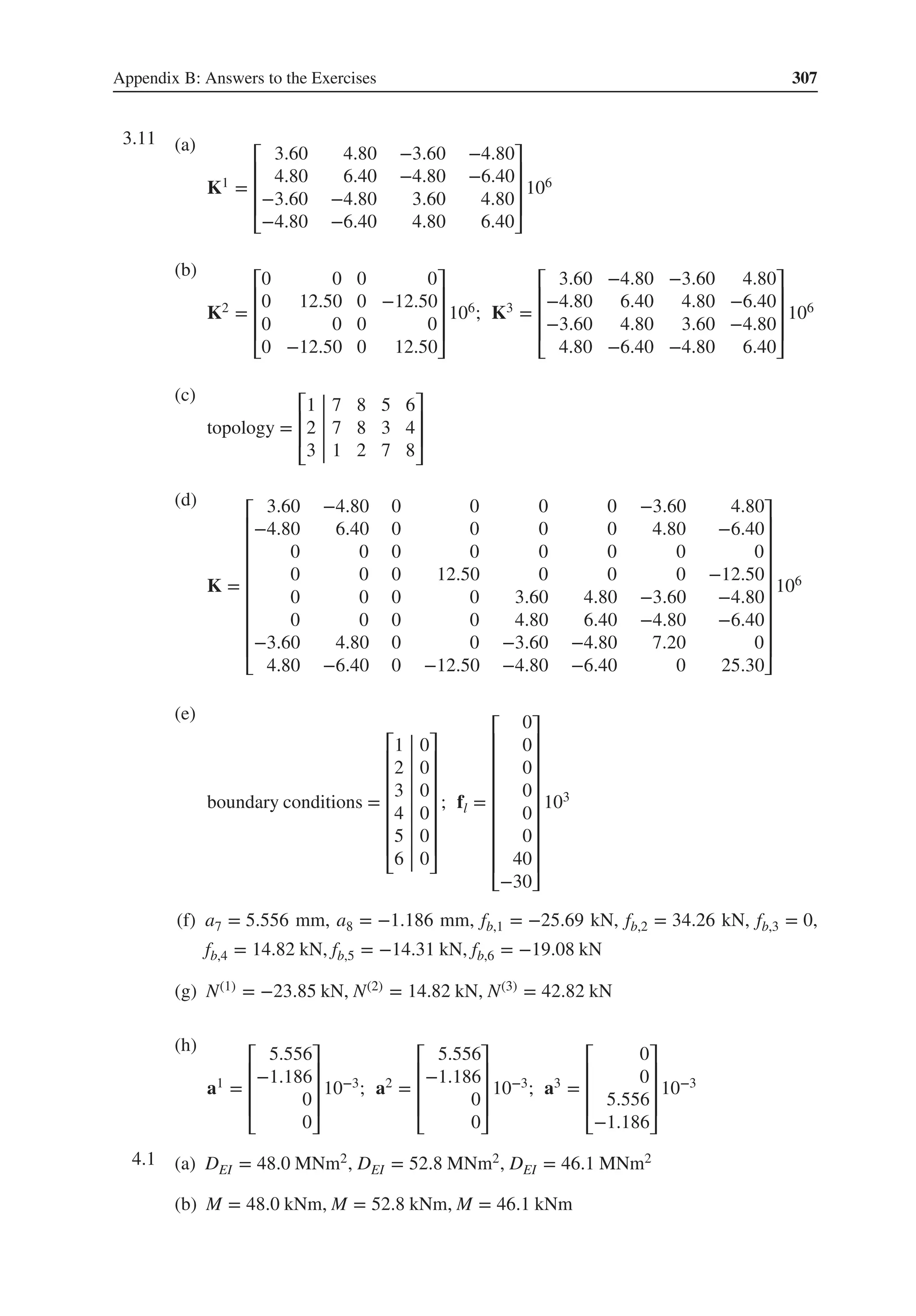
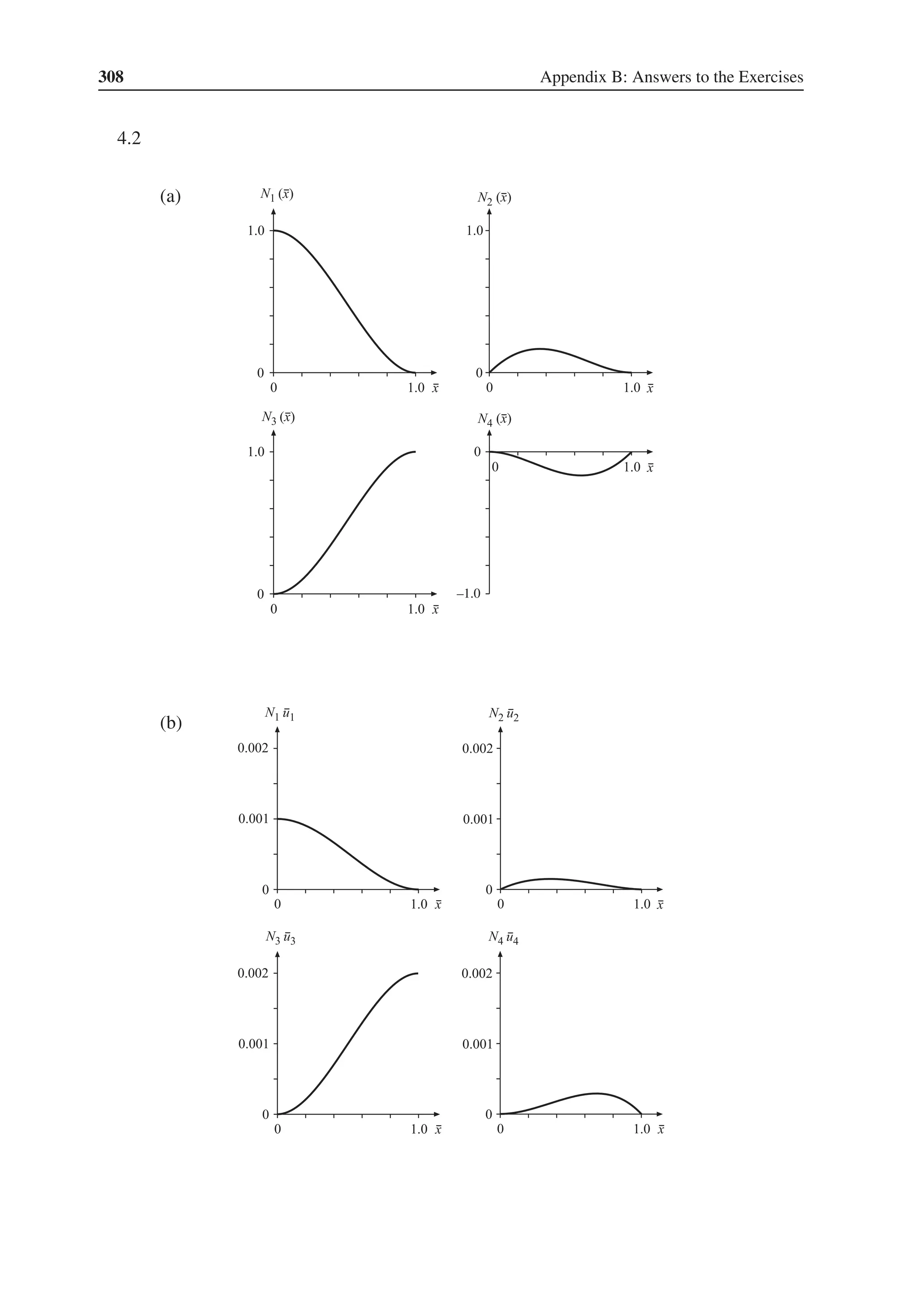
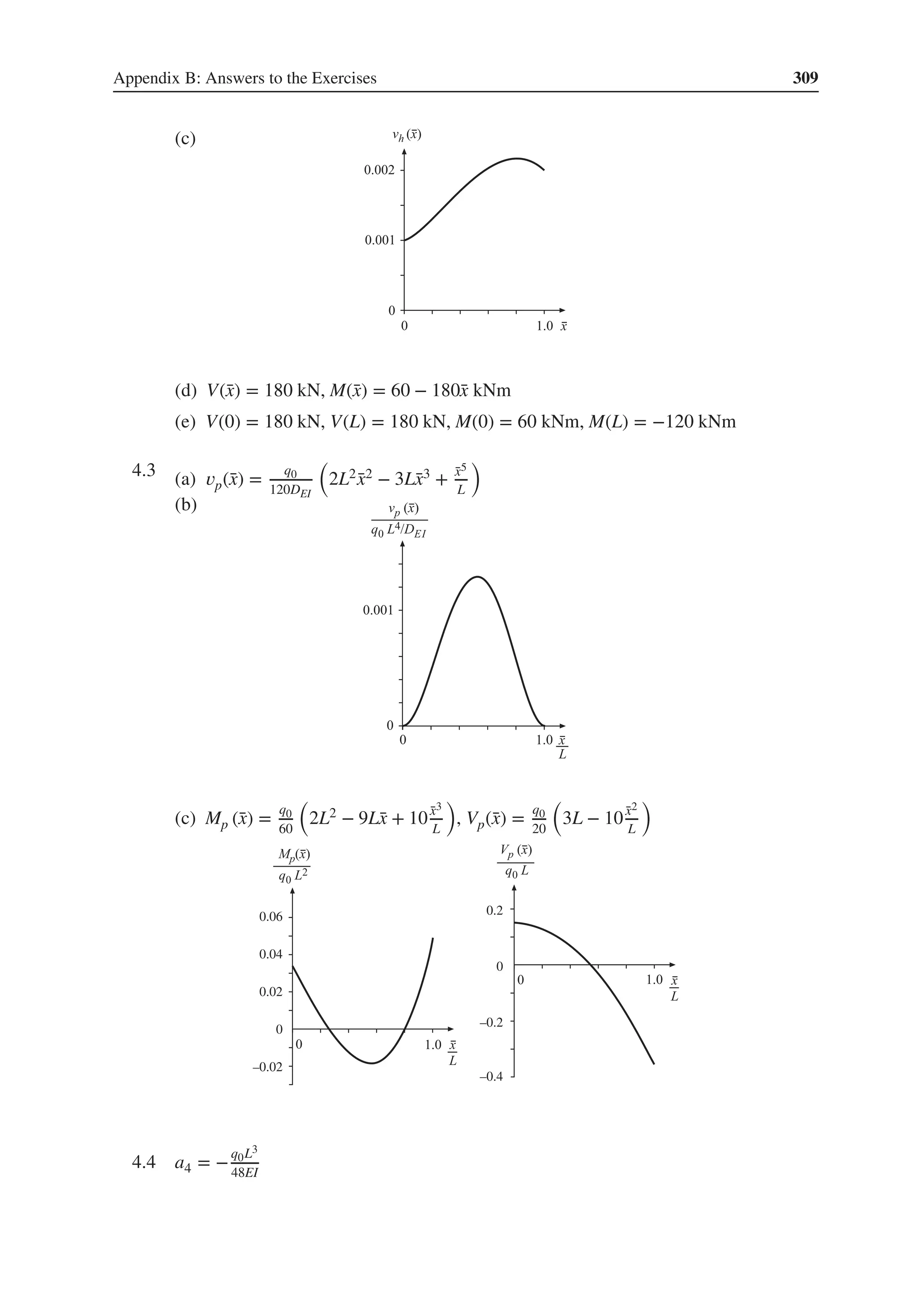
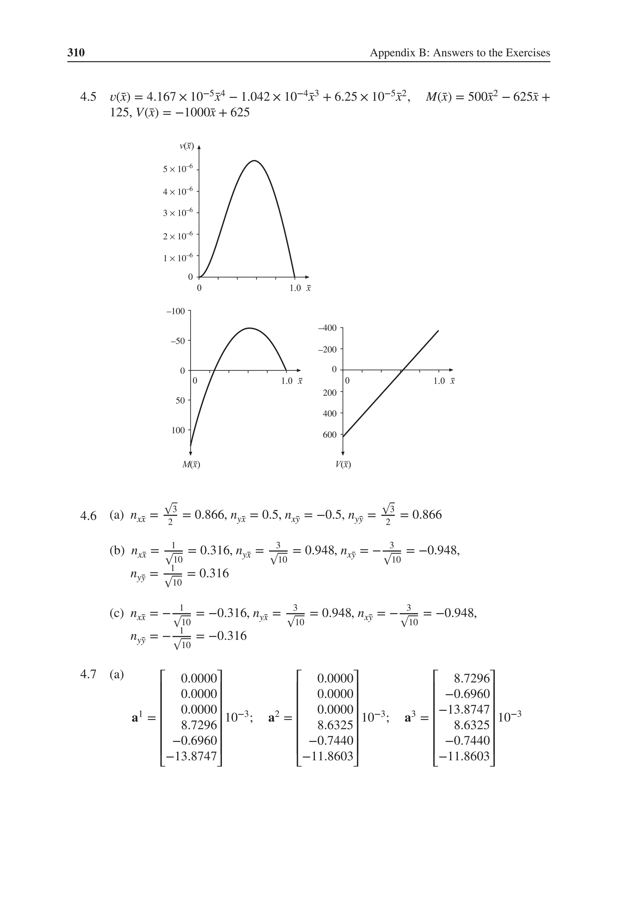
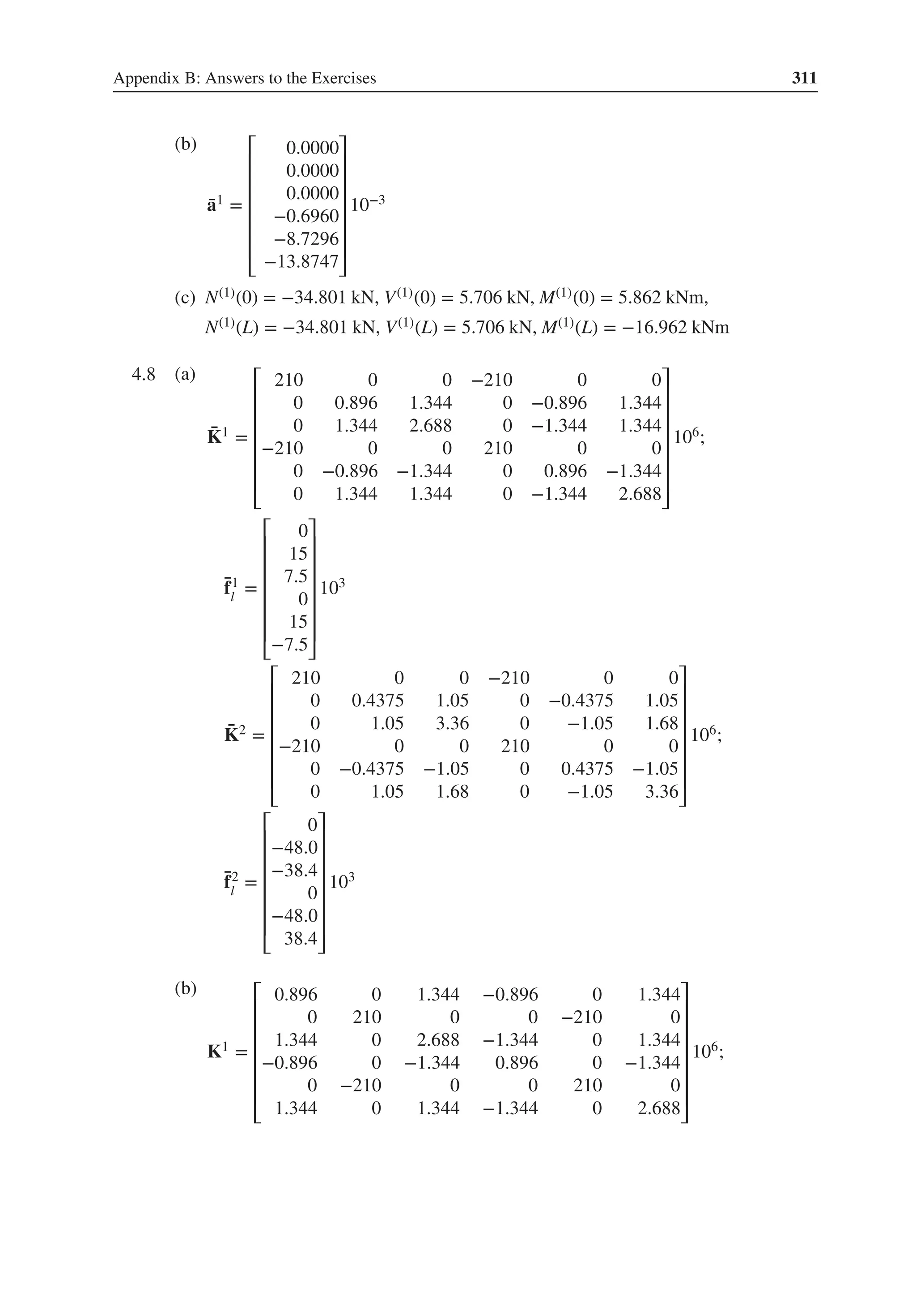
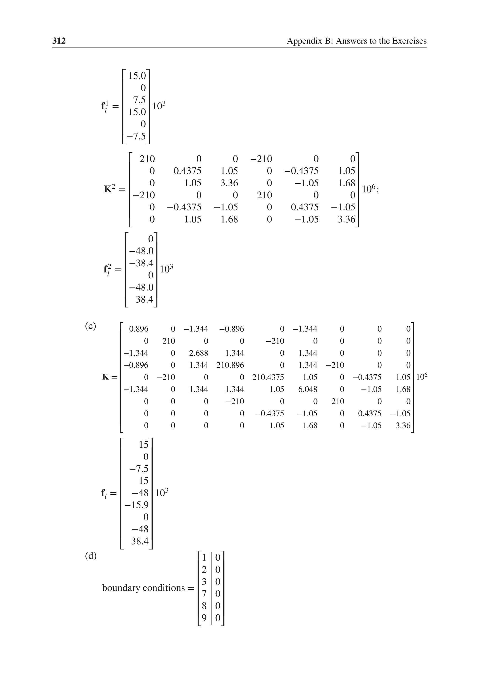

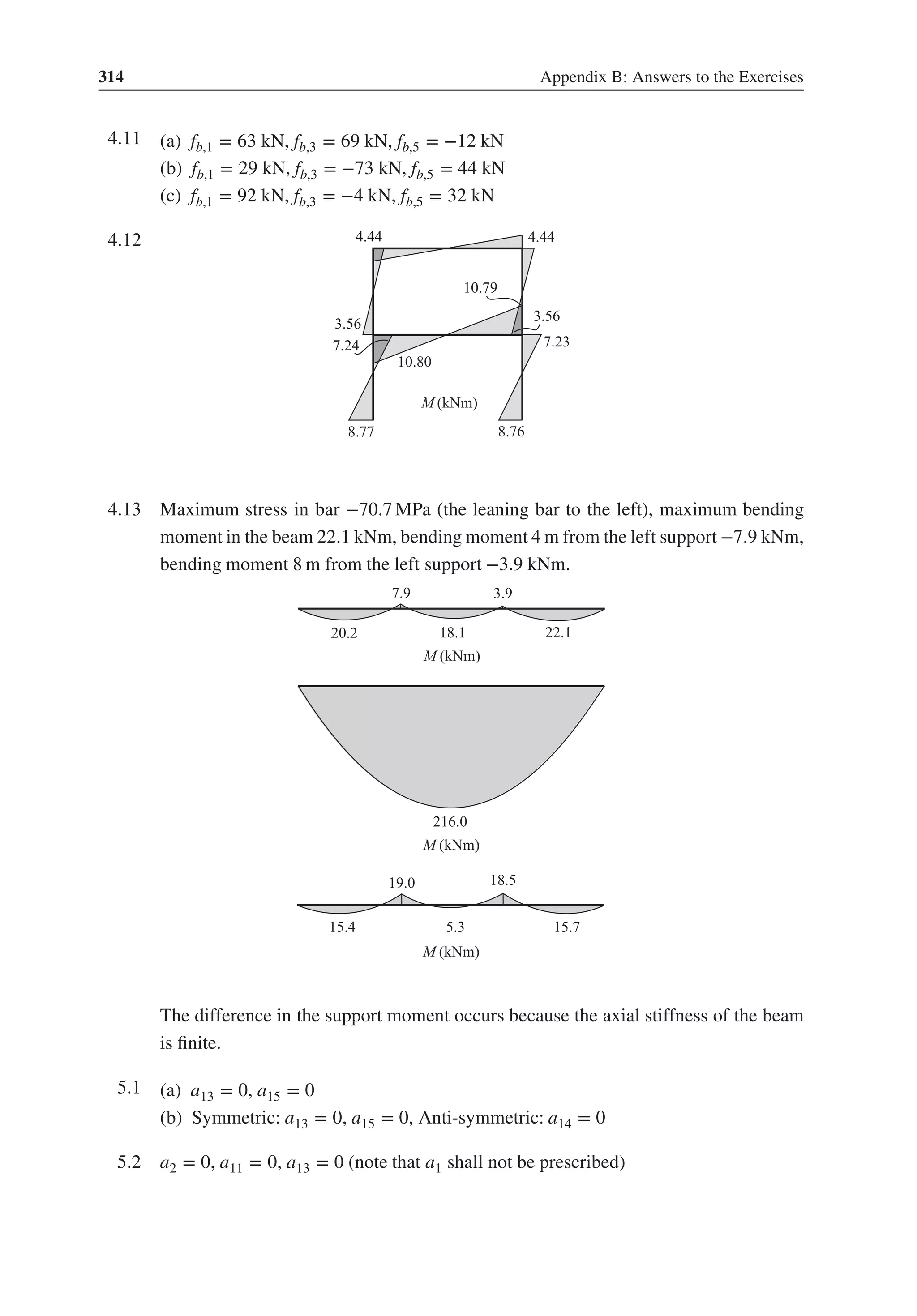
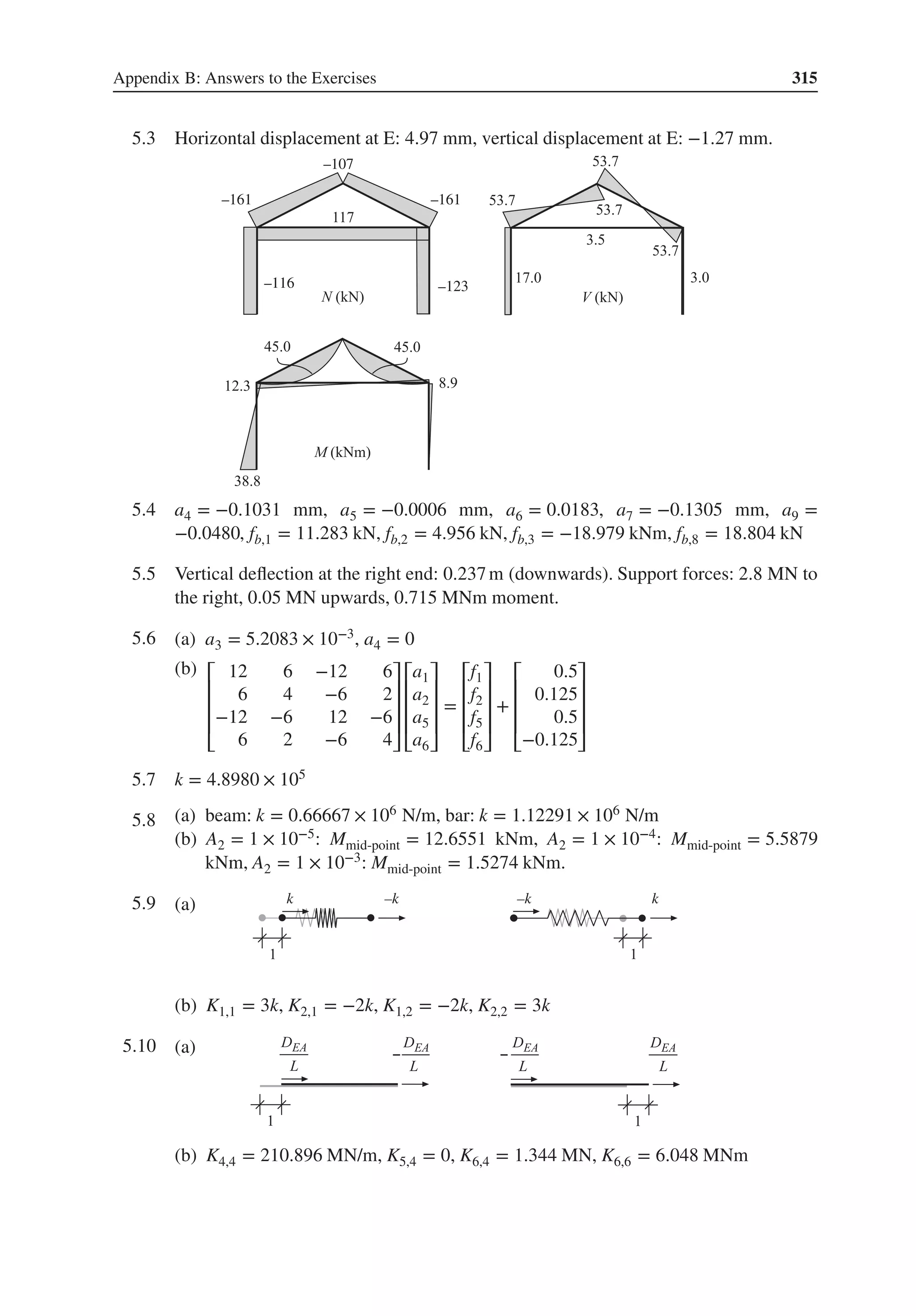

![Appendix B: Answers to the Exercises 317
Four elements
Two elements
7.1
G =
[
0.81111 0.32444 −0.48666 0 0 0
0 0 0 0.81111 0.32444 −0.48666
]
7.2 .
(a) ̄
u(5)
1
= 4.286 mm, ̄
u(5)
2
= 0
(b) change in length = −4.286 mm, N(5) = −173.2 kN, 𝜎(5) = −173.2 MPa
7.3 uA,x = −1.115 mm, uA,y = −6.233 mm, uA,z = 0.874 mm, NAB = 63.74 kN,
NAC = −19.76 kN, NAD = −26.52 kN
7.4 .
(a)
̄
fe
l
=
q𝜔L
2
[
1
1
]
(b) uB =
q0L2
2DGK
7.5
G =
⎡
⎢
⎢
⎢
⎣
C 0 0 0
0 C 0 0
0 0 C 0
0 0 0 C
⎤
⎥
⎥
⎥
⎦
; C =
⎡
⎢
⎢
⎣
0.89443 0.44722 0
−0.44722 0.89443 0
0 0 1.00000
⎤
⎥
⎥
⎦
7.6 .
(a) a13 = 0, a17 = 0, a18 = 0
(b) a14 = 0, a15 = 0, a16 = 0
7.7 Largest vertical displacement at E = 4.541 mm (downwards); Section forces at B:
shear force = 7.014 kN, torque = 0.966 kNm, bending moment = 4.799 kNm (tension
at upper edge); Section forces at C: shear force = 12.986 kN, torque = 0.923 kNm,
bending moment M = 7.308 kNm (tension at upper edge)
8.1 .
(a) K = 8000 MN/m
(b) K = 420 MN/m
(c) K = 2.5 W/m2K
(d) K = 25 W/m2K
(e) K = 0.0833 Ω−1](https://image.slidesharecdn.com/structuralmechanicsmodellingandanalysisofframesandtrussespdfdrive-230720064114-5e1f9a93/75/Structural-mechanics-_-modelling-and-analysis-of-frames-and-trusses-PDFDrive-pdf-331-2048.jpg)