Downloaded 12,558 times


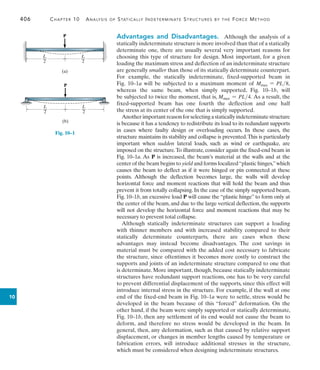
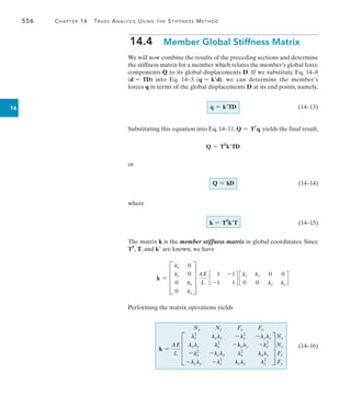
![142 Chapter 4 Internal Loadings Developed in Structural Members
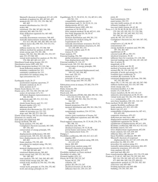
4
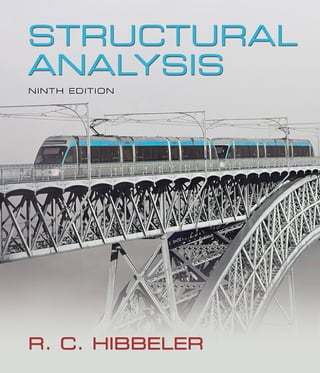
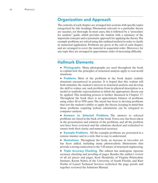
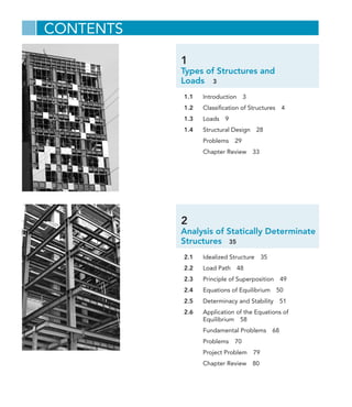
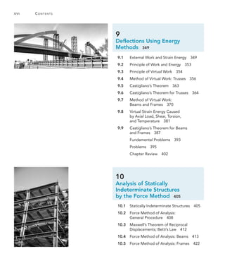
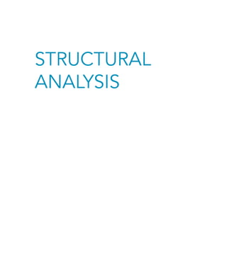
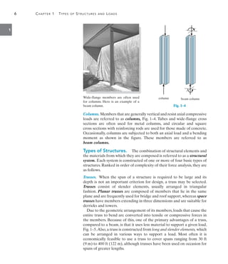
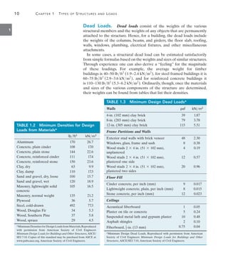
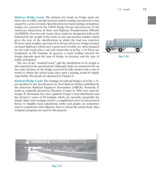
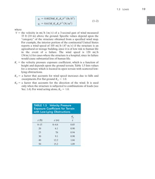
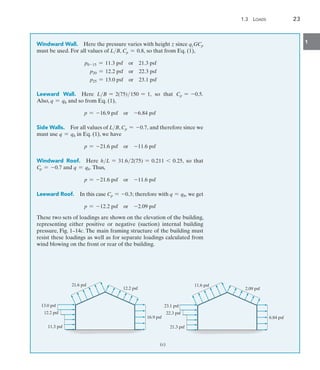
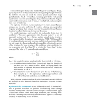
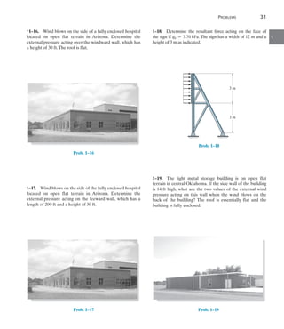
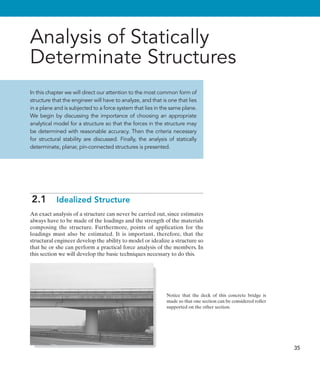
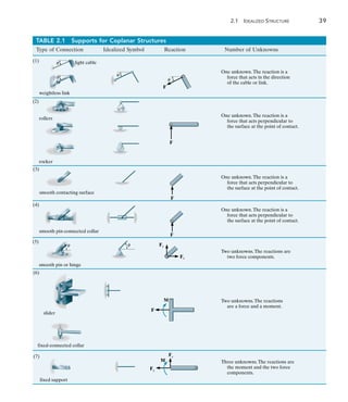
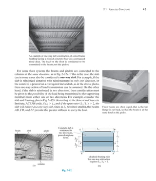
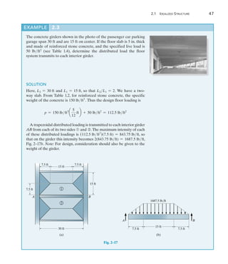
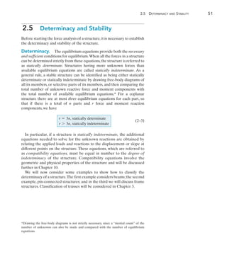
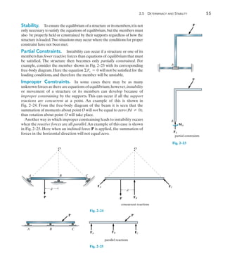
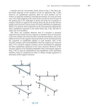
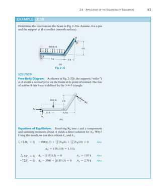
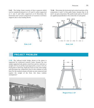
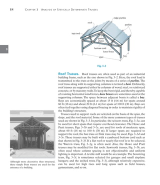
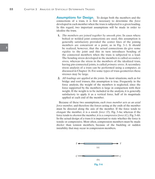
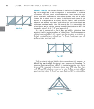
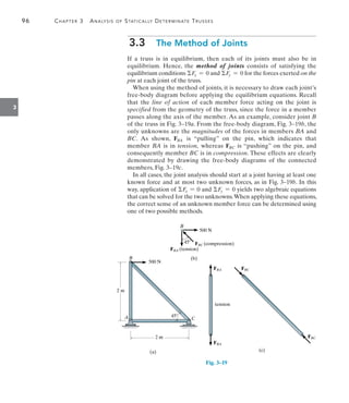
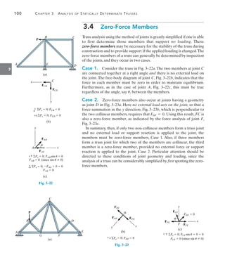
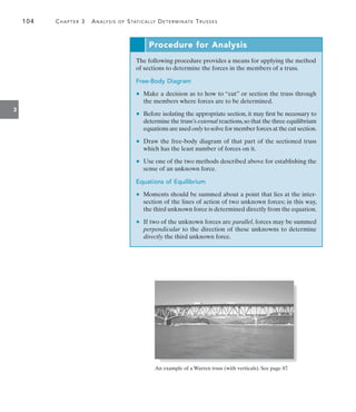
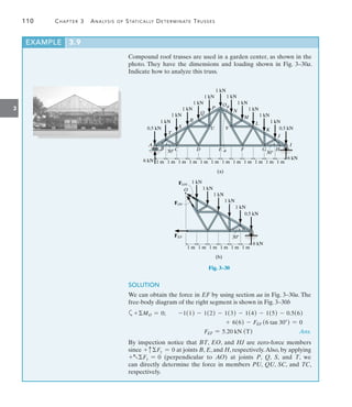
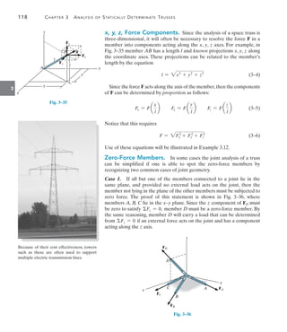
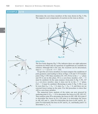
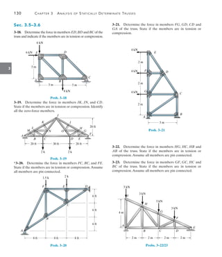
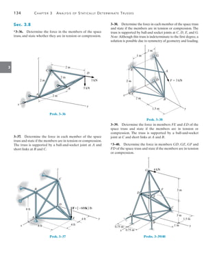
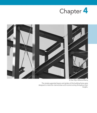
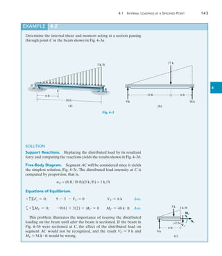
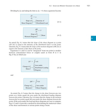
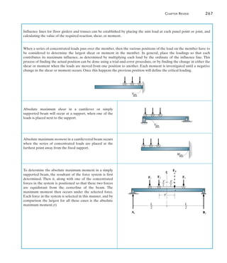
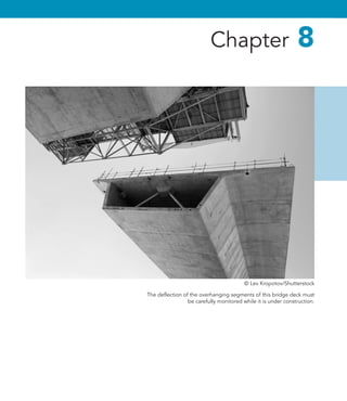
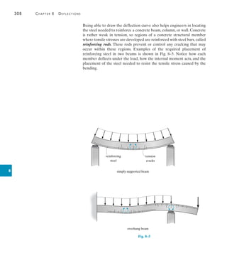
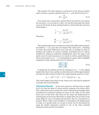
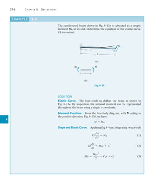
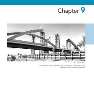
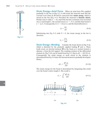
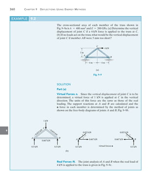
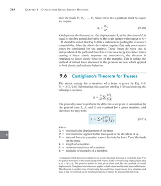
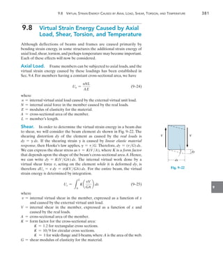
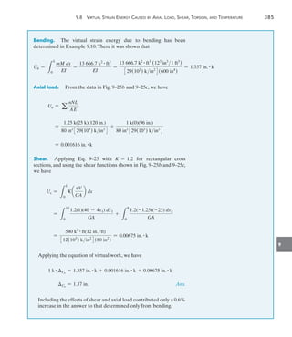
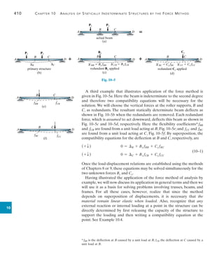
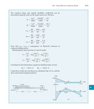
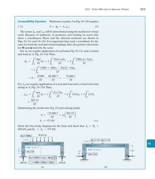
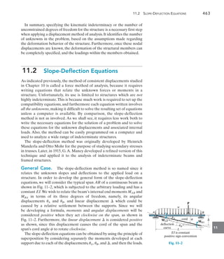
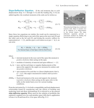
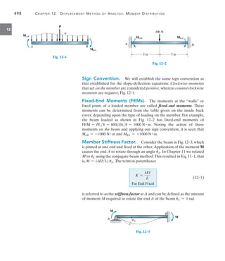
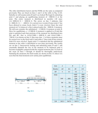
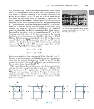
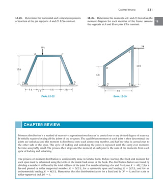
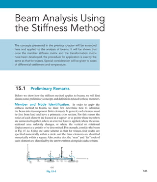
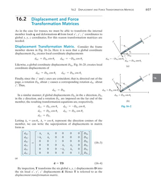
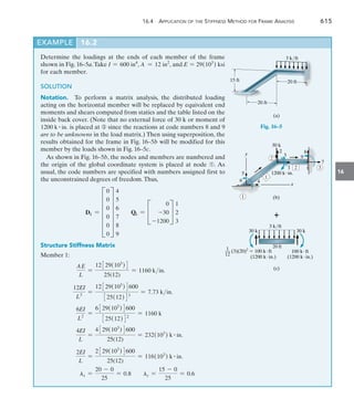
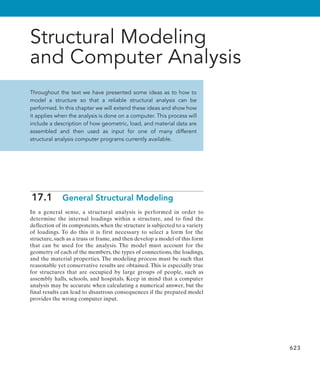
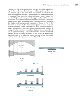
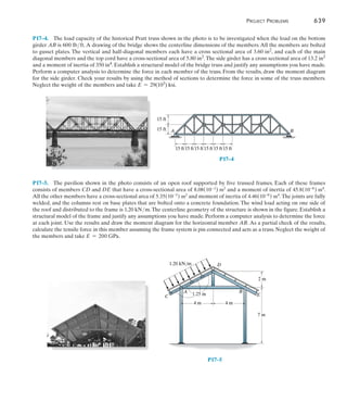
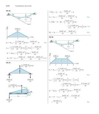
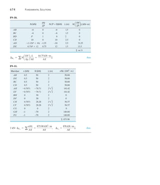
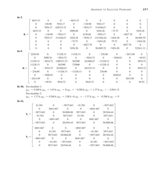
The building roof shown in the photo has a weight of 1.8 kNm2
and is
supported on 8-m long simply supported beams that are spaced 1 m
apart. Each beam, shown in Fig. 4–2b transmits its loading to two
girders, located at the front and back of the building. Determine the
internal shear and moment in the front girder at point C, Fig. 4–2a.
Neglect the weight of the members.
1 m
(a)
1 m 1 m 1 m 1 m 1 m 1 m 1 m 1 m 1 m 1 m 1 m
1.2 m 1.2 m 1.2 m
3.6 kN 3.6 kN
7.2 kN
girder
43.2 kN
43.2 kN
C
7.2 kN 7.2 kN
edge
beam
girder
SOLUTION
Support Reactions. The roof loading is transmitted to each beam
as a one-way slab (L2L1 = 8 m1 m = 8 7 2). The tributary loading
on each interior beam is therefore (1.8 kNm2
)(1 m) = 1.8 kNm.
(The two edge beams support 0.9 kNm.) From Fig. 4–2b, the reaction
of each interior beam on the girder is (1.8 kNm)(8 m)2 = 7.2 kN.
(b) 7.2 kN
beam
0.5 m
0.5 m
1.8 kN/m
7 m
7.2 kN
girder
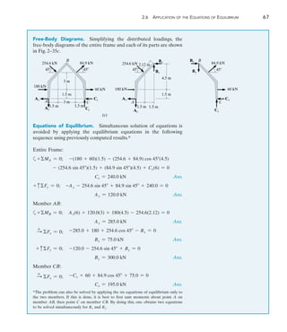
Free-Body Diagram. The free-body diagram of the girder is shown
in Fig. 4–2a. Notice that each column reaction is
[(2(3.6 kN) + 11(7.2 kN)]2 = 43.2 kN
The free-body diagram of the left girder segment is shown in Fig. 4–2c.
Here the internal loadings are assumed to act in their positive directions.
Equations of Equilibrium.
Fig. 4–2
EXAMPLE 4.1
(c)
MC
VC
43.2 kN
1 m 1 m
0.4 m
1.2 m 1.2 m
3.6 kN 7.2 kN 7.2 kN
C
+ cFy = 0; 43.2 - 3.6 - 2(7.2) - VC = 0
VC = 25.2 kN Ans.
a+MC = 0; MC + 7.2(0.4) + 7.2(1.4) + 3.6(2.4) - 43.2(1.2) = 0
MC = 30.2 kN # m Ans.](https://image.slidesharecdn.com/structuralanalysis-hibbelerpdfdrive-220911133905-65f3c8d4/85/STRUCTURAL-ANALYSIS-NINTH-EDITION-R-C-HIBBELER-163-320.jpg)
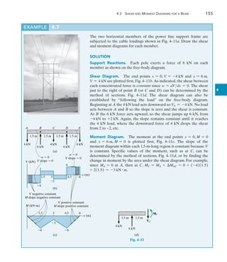
![156 Chapter 4 Internal Loadings Developed in Structural Members
4
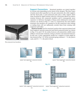
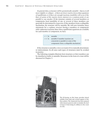
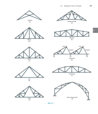
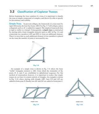
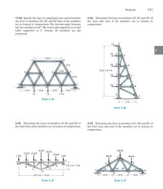
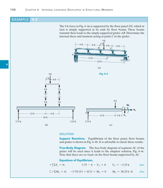
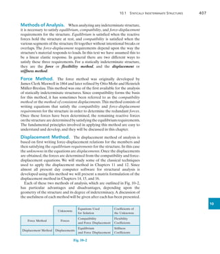
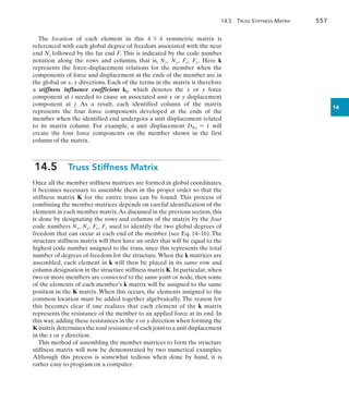
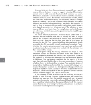
EXAMPLE 4.8
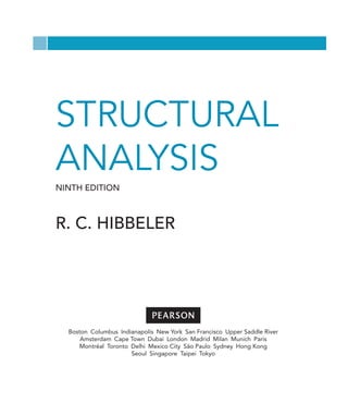
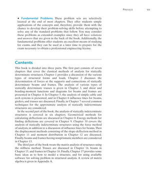
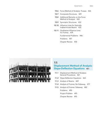
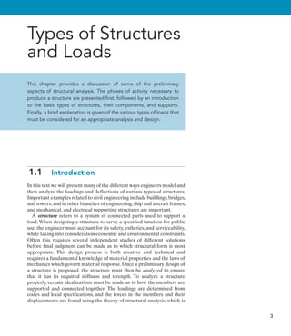
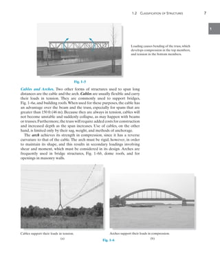
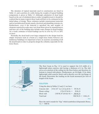
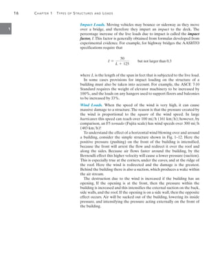
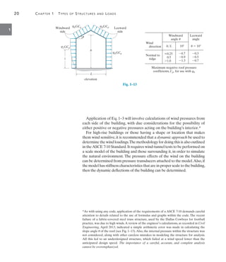
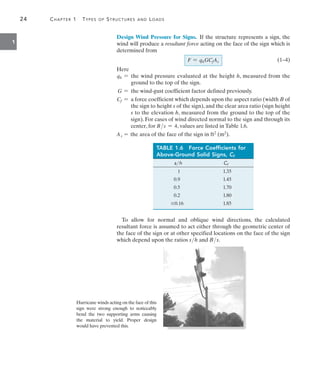
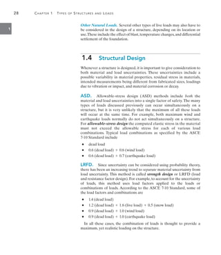
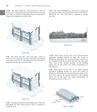
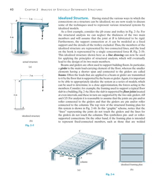
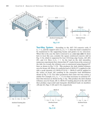
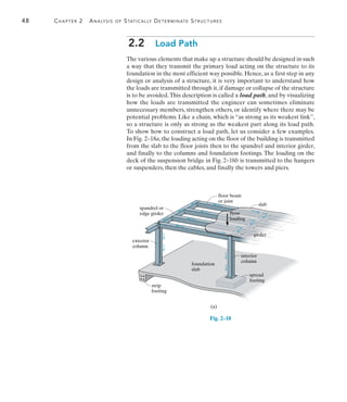
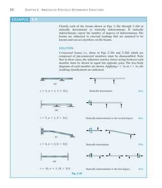
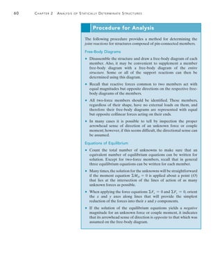
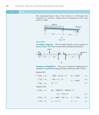
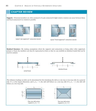
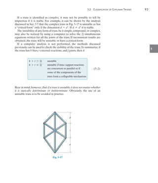
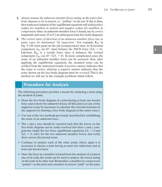
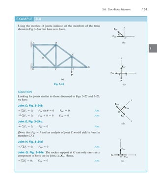
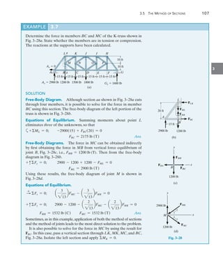
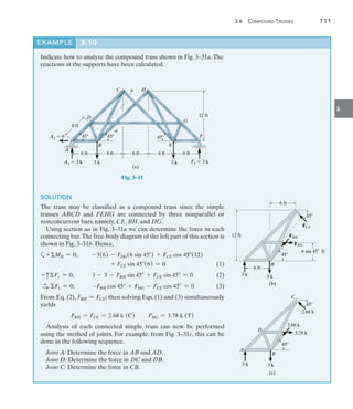
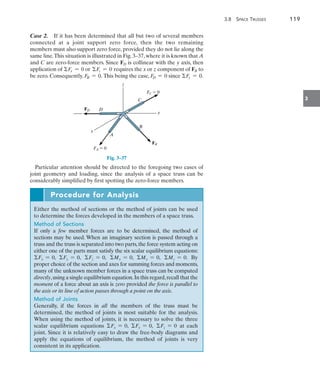
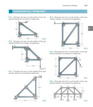
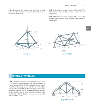
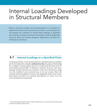
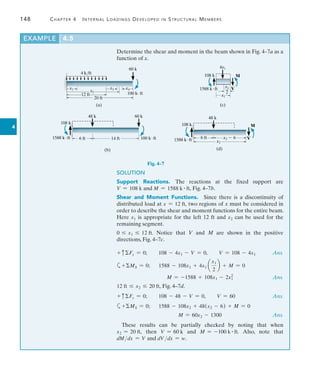
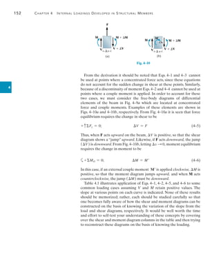
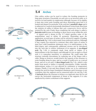
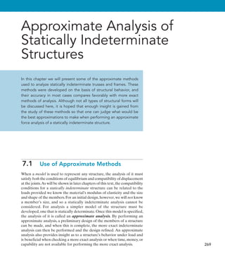
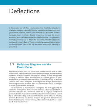
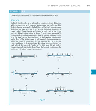
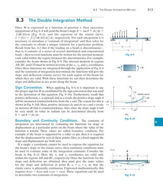
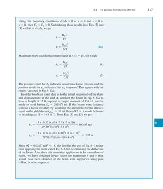
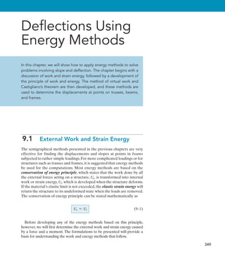
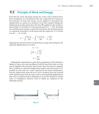
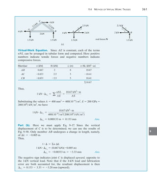
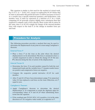
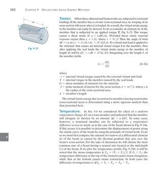
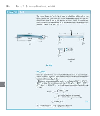
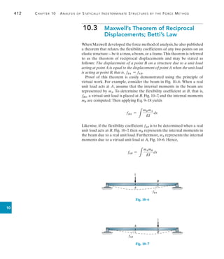
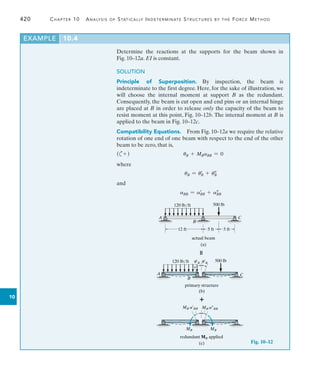
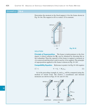
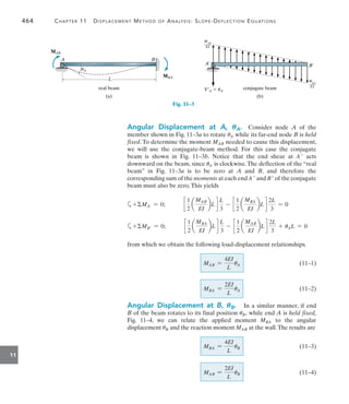
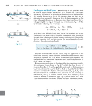
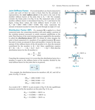
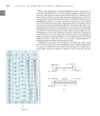
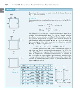
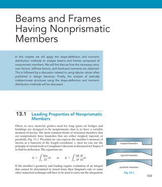
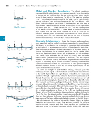
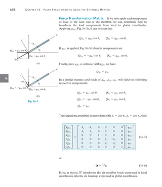
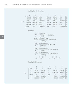
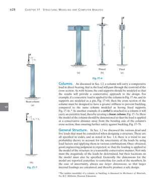
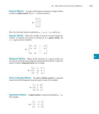
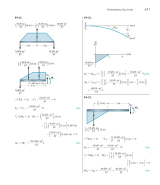
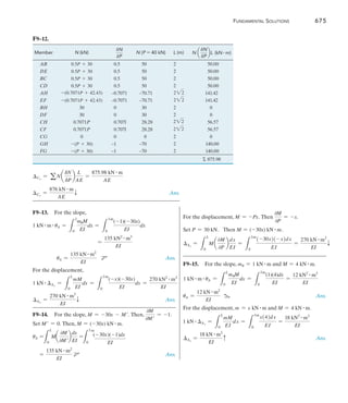
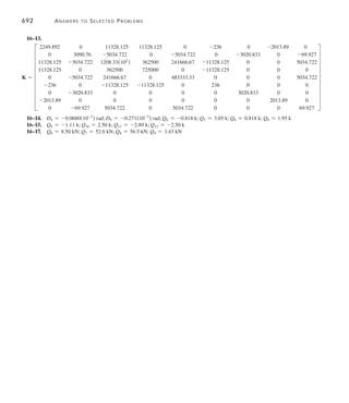
Draw the shear and moment diagrams for the beam in Fig. 4–12a.
9 m
20 kN/m
(a)
Fig. 4–12
SOLUTION
Support Reactions. The reactions have been calculated and are
shown on the free-body diagram of the beam, Fig. 4–12b.
Shear Diagram. The end points x = 0, V = +30 kN and x = 9 m,
V = -60 kN are first plotted. Note that the shear diagram starts with
zero slope since w = 0 at x = 0, and ends with a slope of
w = -20 kNm.
The point of zero shear can be found by using the method of sections
from a beam segment of length x, Fig. 4–12e.We require V = 0, so that
+ cFy = 0; 30 -
1
2
c 20a
x
9
b d x = 0 x = 5.20 m
Moment Diagram. For 0 6 x 6 5.20 m the value of shear is
positive but decreasing and so the slope of the moment diagram is
also positive and decreasing (dMdx = V).At x = 5.20 m, dMdx = 0.
Likewise for 5.20 m 6 x 6 9 m, the shear and so the slope of the
moment diagram are negative increasing as indicated.
The maximum value of moment is at x = 5.20 m since
dMdx = V = 0 at this point,Fig.4–12d.From the free-body diagram in
Fig. 4–12e we have
a+MS = 0; -30(5.20) +
1
2
c 20a
5.20
9
b d (5.20)a
5.20
3
b + M = 0
M = 104 kN # m
V (kN)
30
60
x (m)
(c)
5.20 m
20 kN/m
(b)
30 kN 60 kN
104
M (kNm)
x (m)
(d)
V positive decreasing
M slope positive decreasing
w negative increasing
V slope negative increasing
V negative increasing
M slope negative increasing
(e)
30 kN
[20 ]x
1
—
2
x
—
9
x
—
9
20
V
M
x
x
—
3](https://image.slidesharecdn.com/structuralanalysis-hibbelerpdfdrive-220911133905-65f3c8d4/85/STRUCTURAL-ANALYSIS-NINTH-EDITION-R-C-HIBBELER-177-320.jpg)


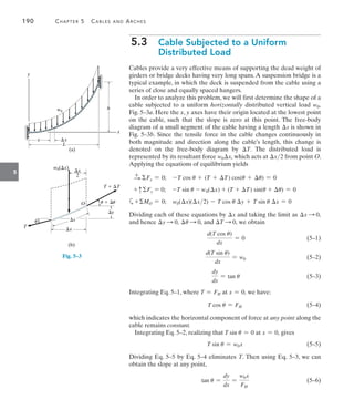
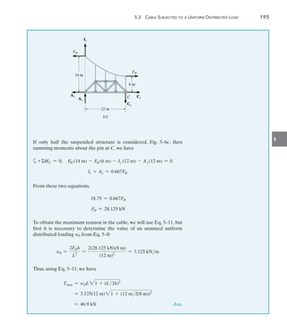
![192 Chapter 5 Cables and Arches
5
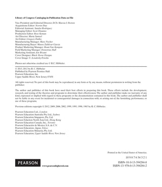
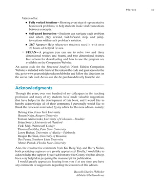
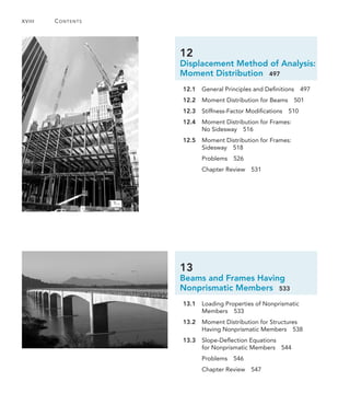
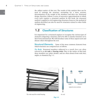
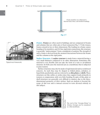
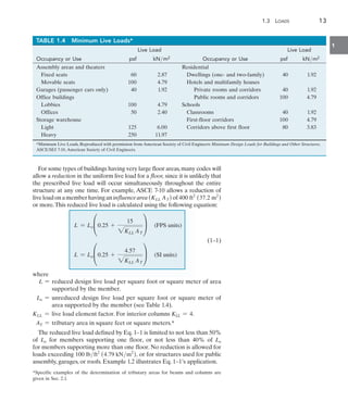
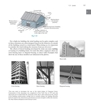
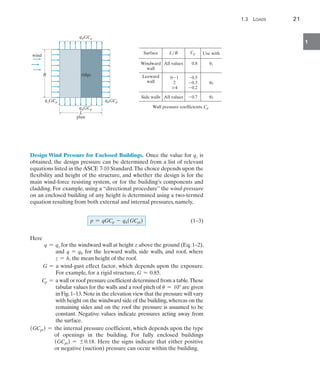
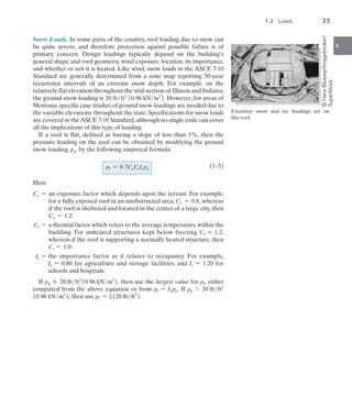
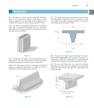
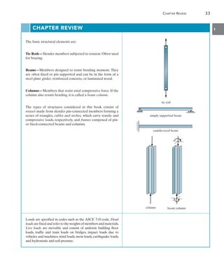
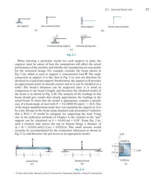
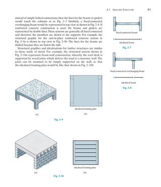
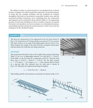
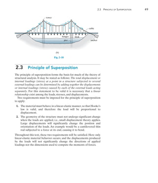
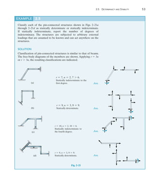
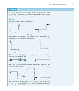
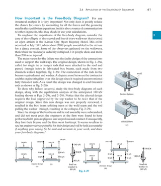
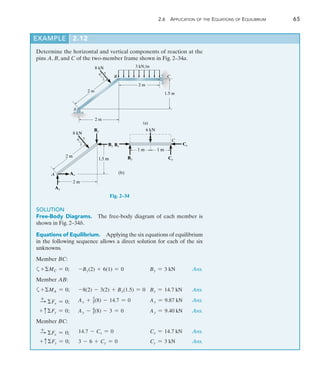
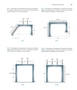
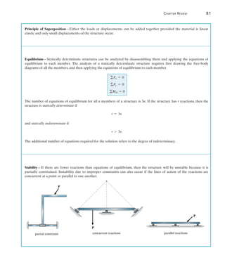
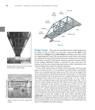
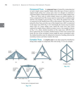
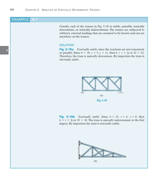
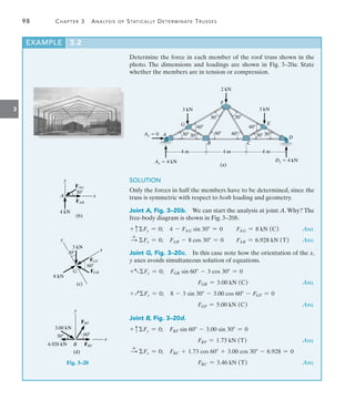
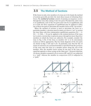
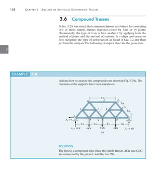
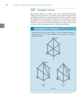
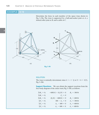
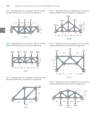
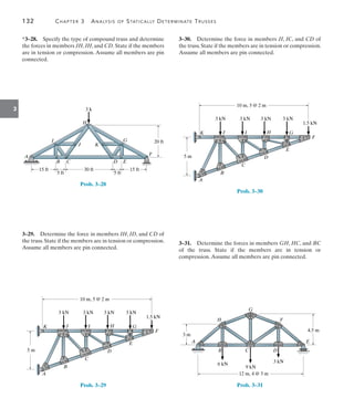
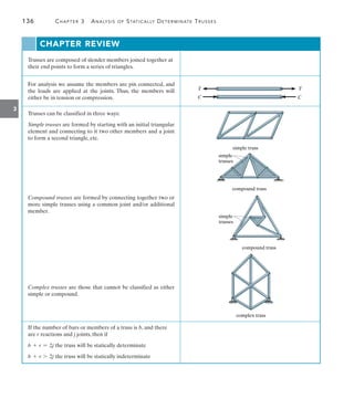
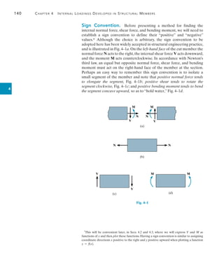
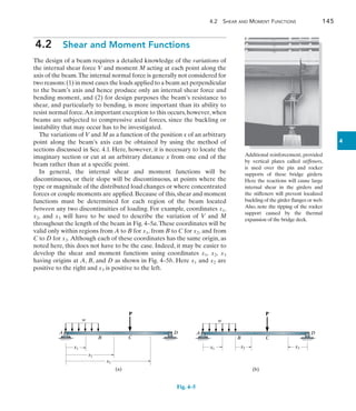
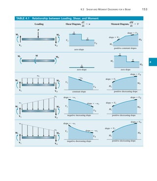
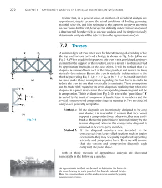
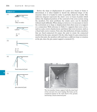
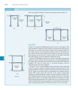
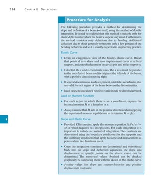
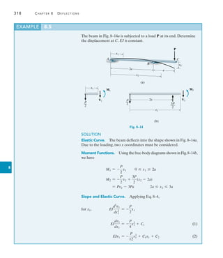
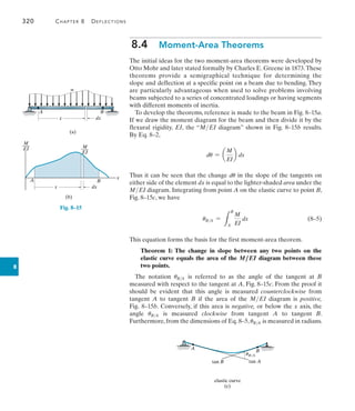
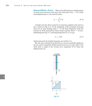
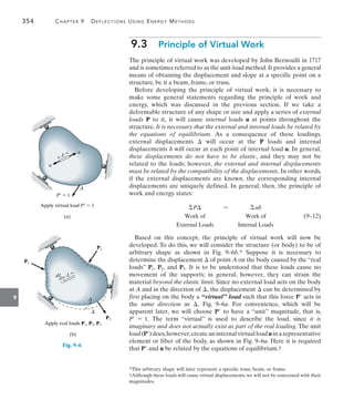
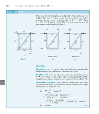
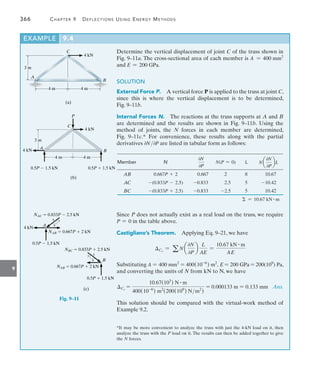
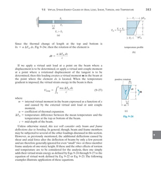
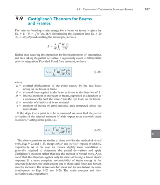
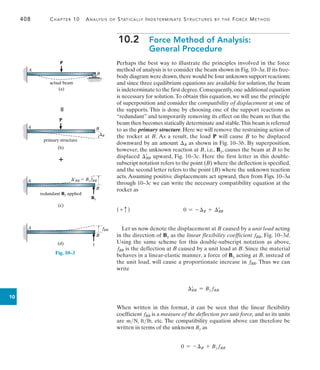
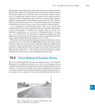
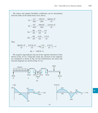
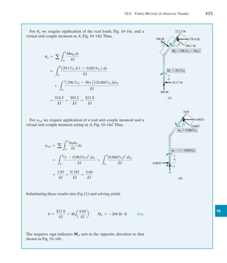
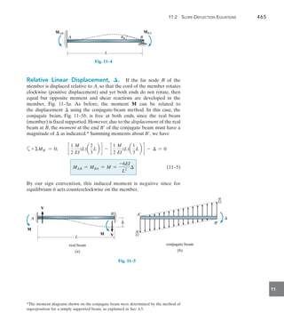
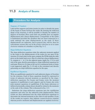
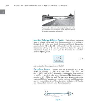
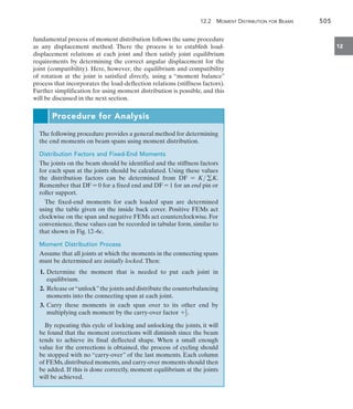
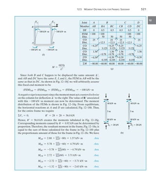
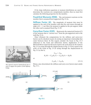
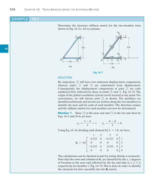
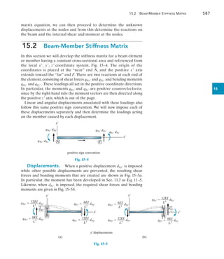
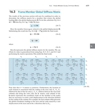
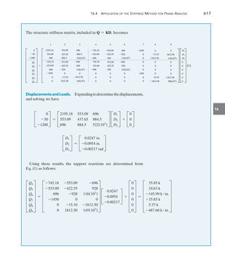
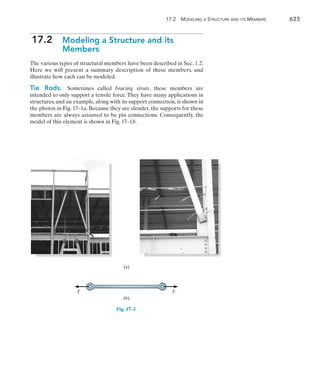
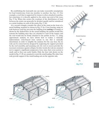
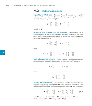
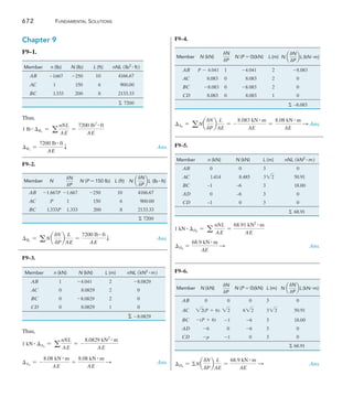
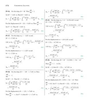
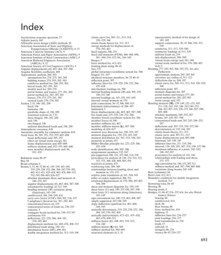
The cable in Fig. 5–5a supports a girder which weighs 850 lbft.
Determine the tension in the cable at points A, B, and C.
EXAMPLE 5.2
C
100 ft
20 ft
(a)
A
B
40 ft
Fig. 5–5
(b)
100 ft x¿
40 ft
20 ft
A
C
B
y
x¿
x
SOLUTION
The origin of the coordinate axes is established at point B, the lowest
point on the cable, where the slope is zero, Fig. 5–5b. From Eq. 5–7, the
parabolic equation for the cable is:
y =
w0
2FH
x2
=
850 lbft
2FH
x2
=
425
FH
x2
(1)
Assuming point C is located x from B, we have
20 =
425
FH
x=2
FH = 21.25x=2
(2)
Also, for point A,
40 =
425
FH
[-(100 - x)]2
40 =
425
21.25x=2
[-(100 - x)]2
x=2
+ 200x - 10 000 = 0
x = 41.42 ft](https://image.slidesharecdn.com/structuralanalysis-hibbelerpdfdrive-220911133905-65f3c8d4/85/STRUCTURAL-ANALYSIS-NINTH-EDITION-R-C-HIBBELER-213-320.jpg)

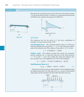
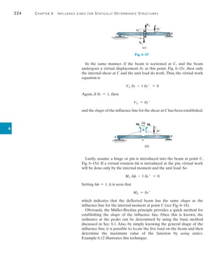
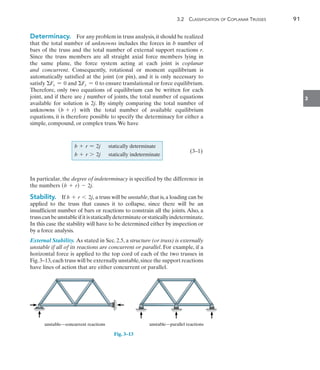
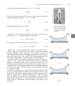
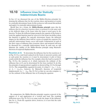
![226 Chapter 6 Influence Lines for Statically Determinate Structures
6
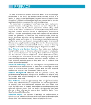
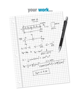
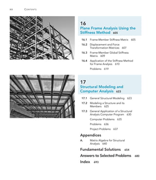
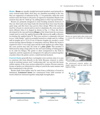
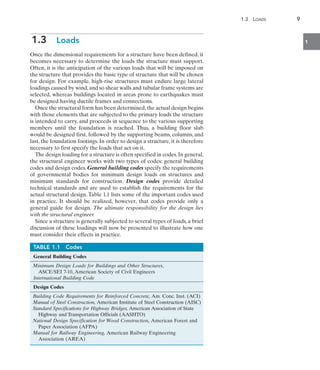
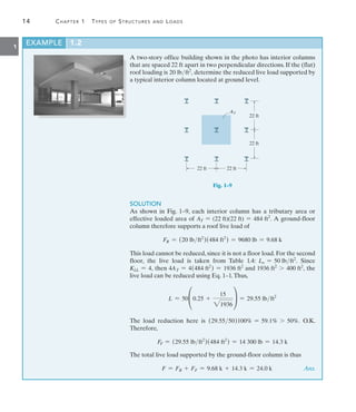
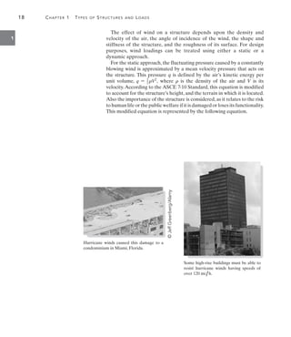
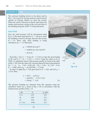
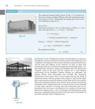
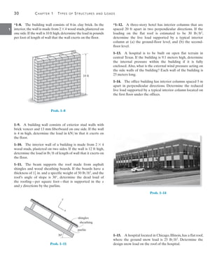
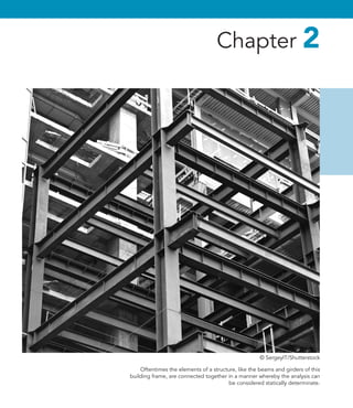
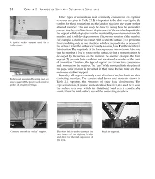
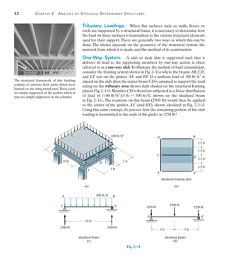
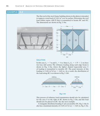
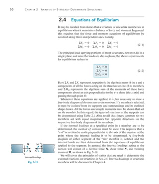
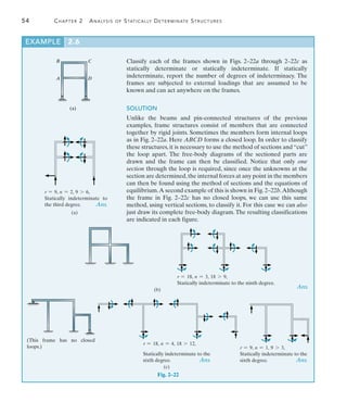
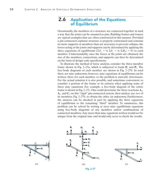
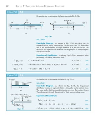
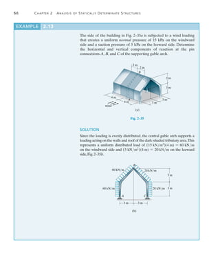
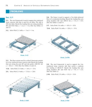
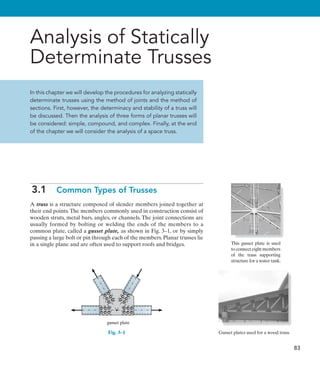
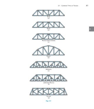
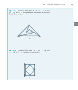
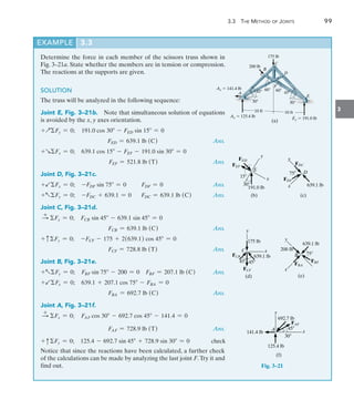
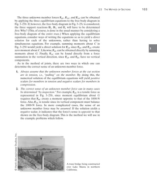
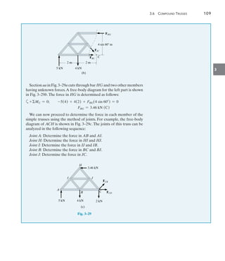
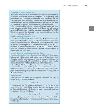
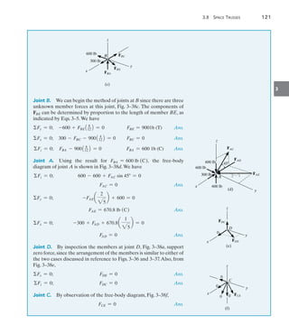
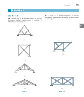
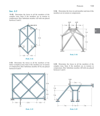
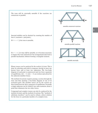
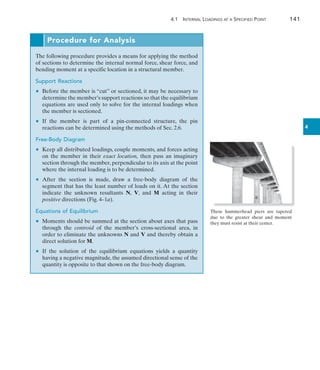
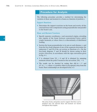
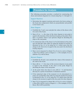
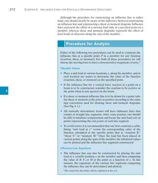
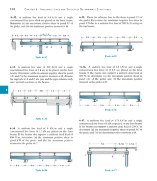
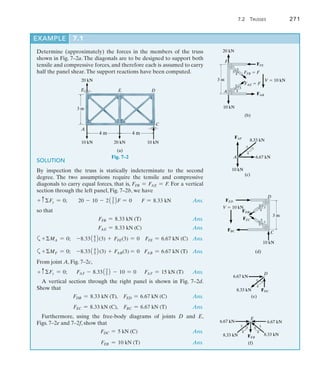
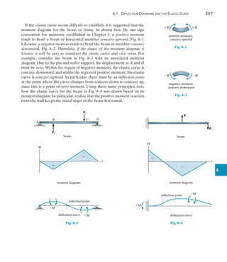
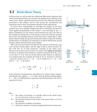
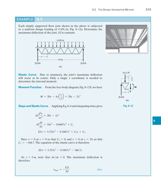
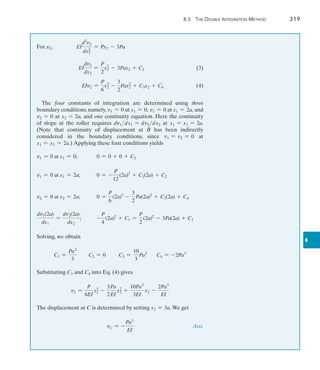
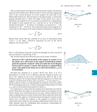
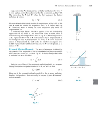
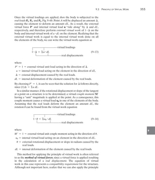
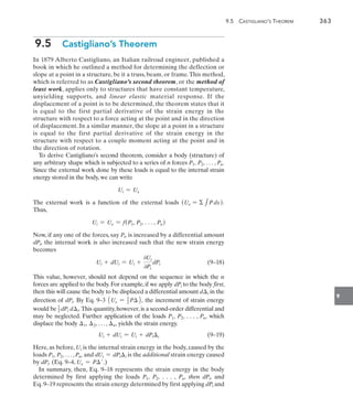
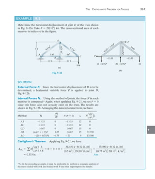
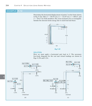
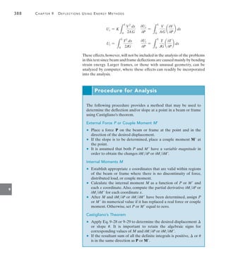
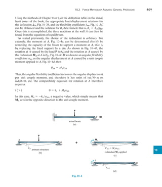
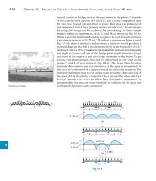
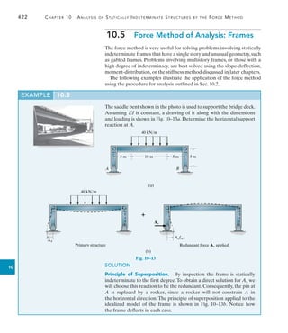
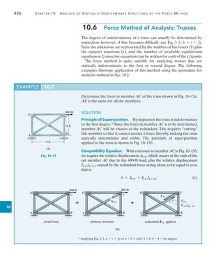
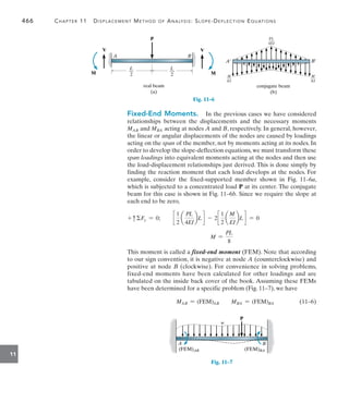
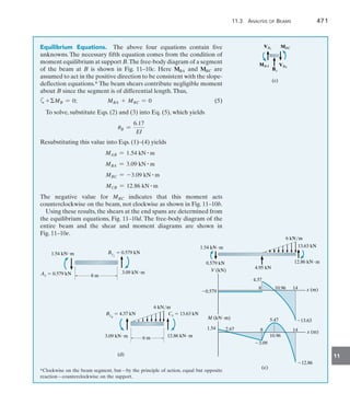
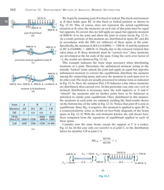
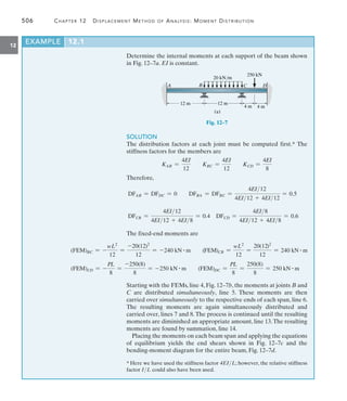
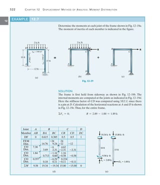
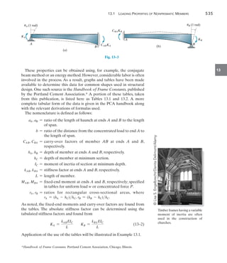
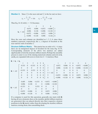
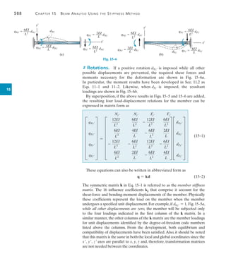
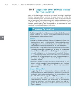
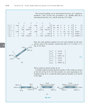
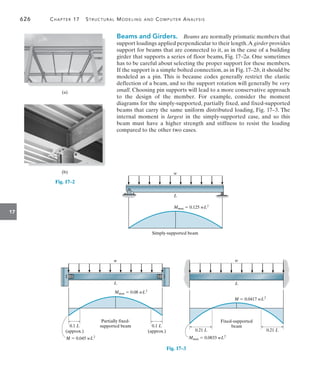
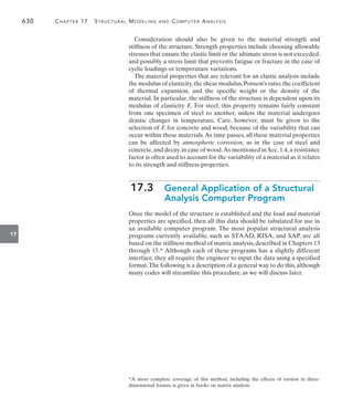
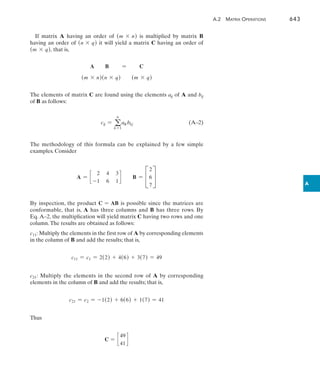
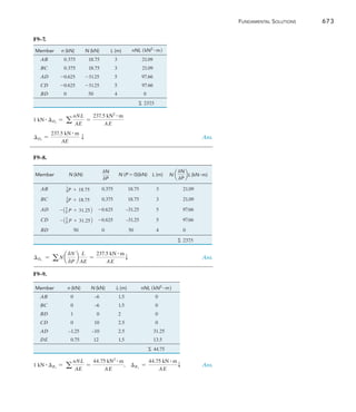
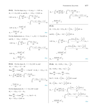
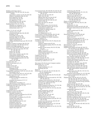
For each beam in Figs. 6–17a through 6–17c, sketch the influence line
for the shear at B.
SOLUTION
The roller guide is introduced at B and the positive shear VB is applied.
Notice that the right segment of the beam will not deflect since the
roller at A actually constrains the beam from moving vertically, either
up or down. [See support (2) in Table 2.1.]
EXAMPLE 6.10
(a)
A
B
VB
VB
A
B
deflected shape
VB
influence line for VB
x
Fig. 6–17
Placing the roller guide at B and applying the positive shear at B
yields the deflected shape and corresponding influence line.
Again, the roller guide is placed at B, the positive shear is applied, and
the deflected shape and corresponding influence line are shown. Note
that the left segment of the beam does not deflect, due to the fixed
support.
B B
VB
VB
deflected shape influence line for VB
VB
x
(c)
B B
VB
VB
deflected shape influence line for VB
VB
x
(b)](https://image.slidesharecdn.com/structuralanalysis-hibbelerpdfdrive-220911133905-65f3c8d4/85/STRUCTURAL-ANALYSIS-NINTH-EDITION-R-C-HIBBELER-247-320.jpg)
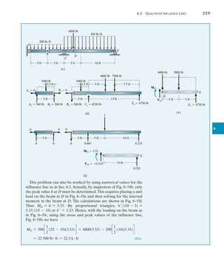
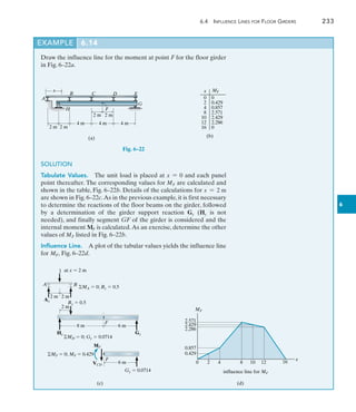
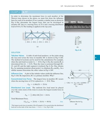
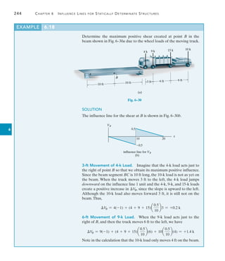
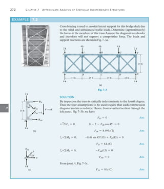
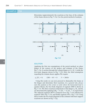
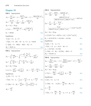
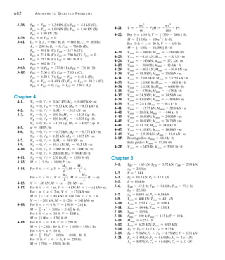
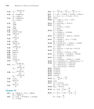
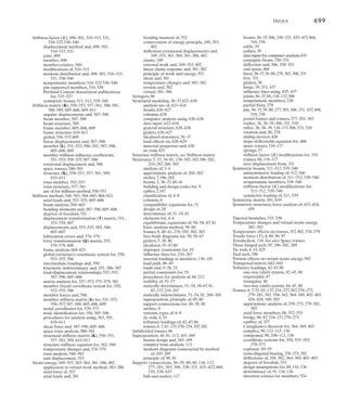
(5) = +0.125 k
Since this result is positive, Case 2 will yield a larger value for VC than
Case 1. [Compare the answers for (VC)1 and (VC)2 previously calculated,
where indeed (VC)2 = (VC)1 + 0.125.] Investigating V293, which occurs
when Case 2 moves to Case 3, Fig. 6–28b, we must account for the
downward (negative) jump of the 4-k load and the 5-ft horizontal
movement of all the loads up the slope of the influence line.We have
V2-3 = 4(-1) + (1 + 4 + 4)(0.025)(5) = -2.875 k
Since V293 is negative, Case 2 is the position of the critical loading, as
determined previously.](https://image.slidesharecdn.com/structuralanalysis-hibbelerpdfdrive-220911133905-65f3c8d4/85/STRUCTURAL-ANALYSIS-NINTH-EDITION-R-C-HIBBELER-261-320.jpg)
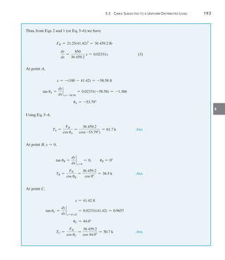
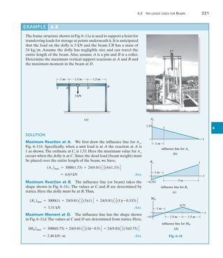
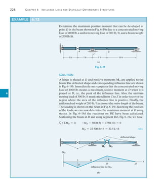
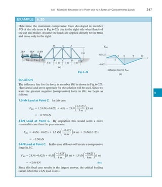
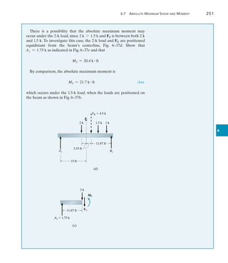
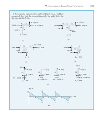
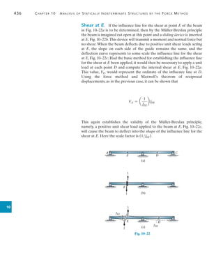
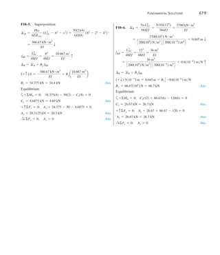
![242 Chapter 6 Influence Lines for Statically Determinate Structures
6
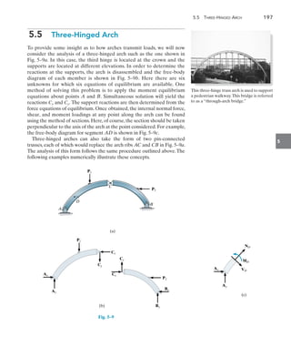
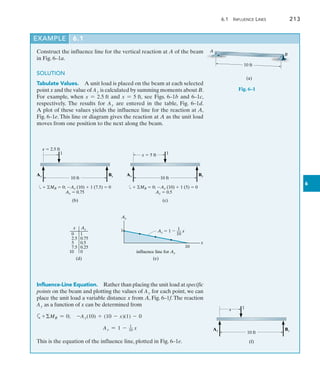
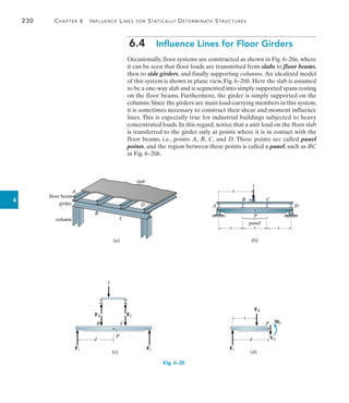
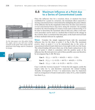
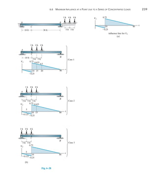
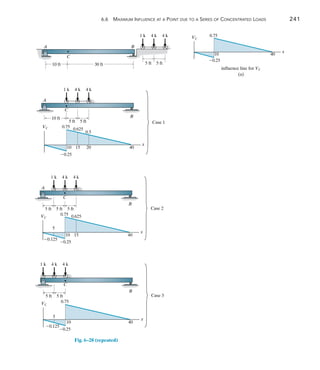
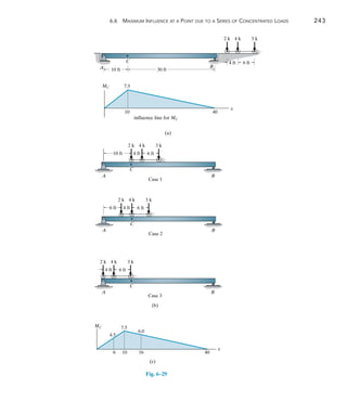
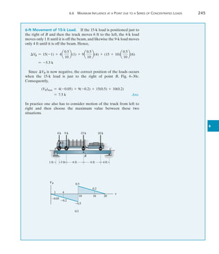
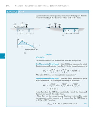
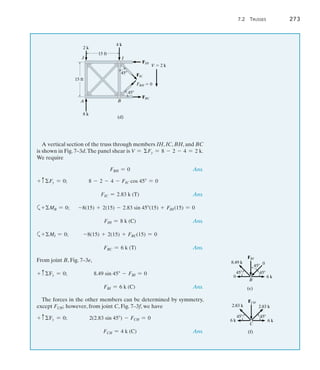
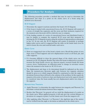
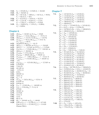
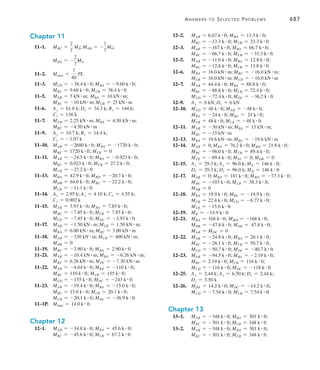
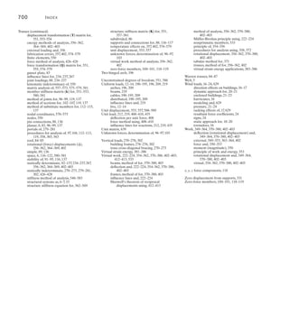
Moment. We can also use the foregoing methods to determine the
critical position of a series of concentrated forces so that they create the
largest internal moment at a specific point in a structure. Of course, it is
first necessary to draw the influence line for the moment at the point.
As an example, consider the beam, loading, and influence line for the
moment at point C in Fig. 6–29a. If each of the three concentrated forces
is placed on the beam, coincident with the peak of the influence line, we
will obtain the greatest influence from each force. The three cases of
loading are shown in Fig. 6–29b.When the loads of Case 1 are moved 4 ft
to the left to Case 2, it is observed that the 2-k load decreases M1-2,
since the slope (7.510) is downward, Fig. 6–29a. Likewise, the 4-k and
3-k forces cause an increase of M1-2, since the slope [7.5(40 - 10)] is
upward.We have
M1-2 = -2a
7.5
10
b(4) + (4 + 3)a
7.5
40 - 10
b(4) = 1.0 k # ft
Since M1-2 is positive, we must further investigate moving the loads 6 ft
from Case 2 to Case 3.
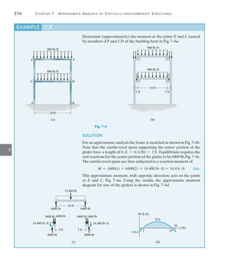
M2-3 = -(2 + 4)a
7.5
10
b(6) + 3a
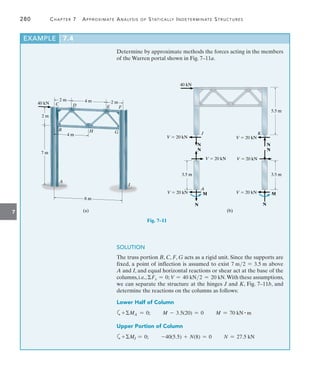
7.5
40 - 10
b(6) = -22.5 k # ft
Here the change is negative, so the greatest moment at C will occur when
the beam is loaded as shown in Case 2, Fig. 6–29c.The maximum moment
at C is therefore
(MC)max = 2(4.5) + 4(7.5) + 3(6.0) = 57.0 k # ft
The following examples further illustrate this method.
The girders of this bridge must resist the
maximum moment caused by the weight of
this jet plane as it passes over it.](https://image.slidesharecdn.com/structuralanalysis-hibbelerpdfdrive-220911133905-65f3c8d4/85/STRUCTURAL-ANALYSIS-NINTH-EDITION-R-C-HIBBELER-263-320.jpg)

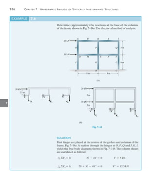
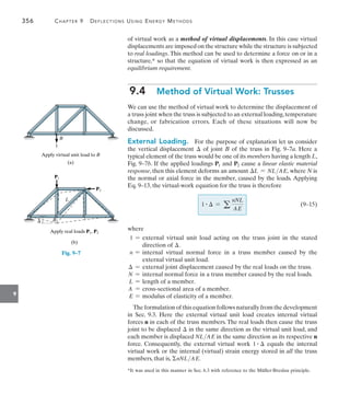
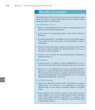
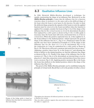
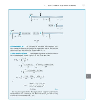
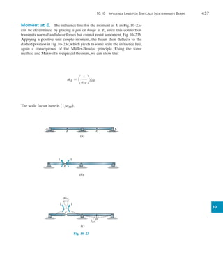
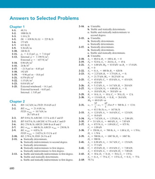
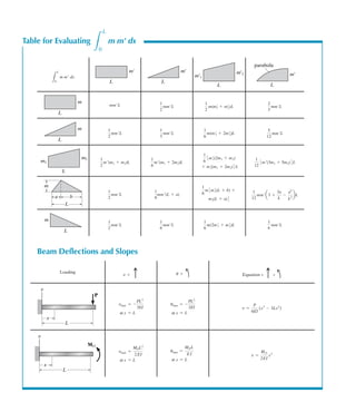
![9
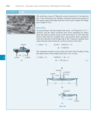
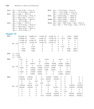
9.7 Method of Virtual Work: Beams and Frames 375
3 kN
A
B
x1 x2 x1
M1 3x1
V1
3 kN
(c)
real load
x2
5 m
B
M2 3 (5 x2)
V2
3 kN
C
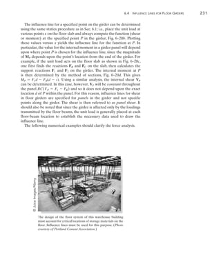
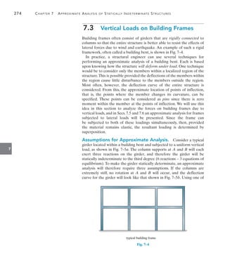
Real Moments M. Using the same coordinates x1 and x2, the
internal moments M are computed as shown in Fig. 9–18c.
Virtual-Work Equation. The slope at B is thus given by
1 # uB =
L
L
0
muM
EI
dx
=
L
5
0
(0)(-3x1) dx1
EI
+
L
5
0
(1)[-3(5 + x2)] dx2
EI
uB =
-112.5 kN # m2
EI
(1)
We can also evaluate the integrals 1muM dx graphically, using the
table given on the inside front cover of the book. To do so it is first
necessary to draw the moment diagrams for the beams in Figs. 9–18b
and 9–18c. These are shown in Figs. 9–18d and 9–18e, respectively.
Since there is no moment m for 0 … x 6 5 m, we use only the shaded
rectangular and trapezoidal areas to evaluate the integral. Finding
these shapes in the appropriate row and column of the table, we have
L
10
5
muM dx = 1
2 mu(M1 + M2)L = 1
2 (1)(-15 - 30)5
= -112.5 kN2 # m3
This is the same value as that determined in Eq. 1.Thus,
(1 kN # m) # uB =
-112.5 kN2 # m3
200(106
) kNm2
360(106
) mm4
4(10-12
m4
mm4
)
uB = -0.00938 rad Ans.
The negative sign indicates uB is opposite to the direction of the virtual
couple moment shown in Fig. 9–18b.
5 10
1
x (m)
(d)
mu (kNm)
5 10
M (kNm)
x (m)
(e)
15
30](https://image.slidesharecdn.com/structuralanalysis-hibbelerpdfdrive-220911133905-65f3c8d4/85/STRUCTURAL-ANALYSIS-NINTH-EDITION-R-C-HIBBELER-396-320.jpg)
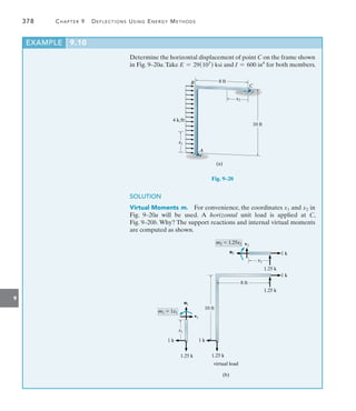


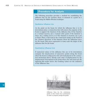
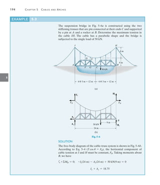
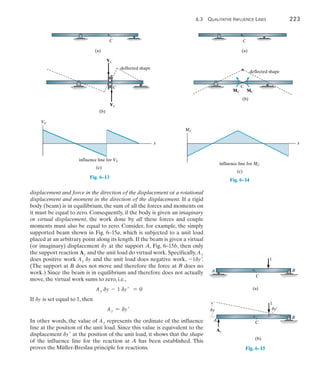
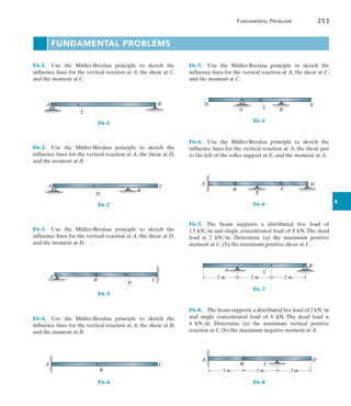
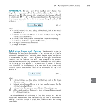
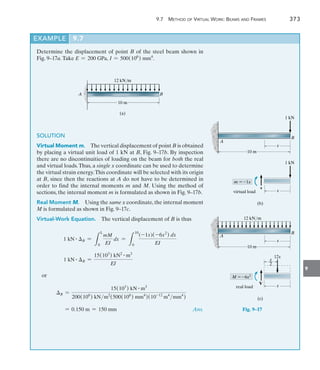
![470 Chapter 11 Displacement Method of Analysis: Slope-Deflection Equations
11
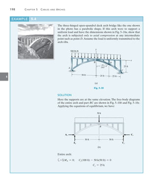
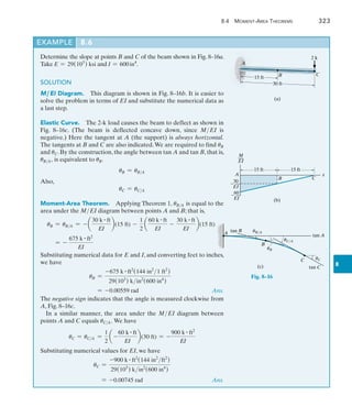
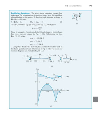
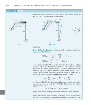
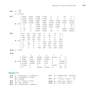
Draw the shear and moment diagrams for the beam shown in
Fig. 11–10a. EI is constant.
SOLUTION
Slope-Deflection Equations. Two spans must be considered in this
problem. Since there is no span having the far end pinned or roller
supported, Eq. 11–8 applies to the solution. Using the formulas for the
FEMs tabulated for the triangular loading given on the inside back
cover, we have
(FEM)BC = -
wL2
30
= -
6(6)2
30
= -7.2 kN # m
(FEM)CB =
wL2
20
=
6(6)2
20
= 10.8 kN # m
Note that (FEM)BC is negative since it acts counterclockwise on the
beam at B. Also, (FEM)AB = (FEM)BA = 0 since there is no load on
span AB.
In order to identify the unknowns, the elastic curve for the beam is
shown in Fig. 11–10b. As indicated, there are four unknown internal
moments. Only the slope at B, uB, is unknown. Since A and C are fixed
supports, uA = uC = 0. Also, since the supports do not settle, nor are
they displaced up or down, cAB = cBC = 0. For span AB, considering
A to be the near end and B to be the far end, we have
MN = 2Ea
I
L
b(2uN + uF - 3c) + (FEM)N
MAB = 2Ea
I
8
b[2(0) + uB - 3(0)] + 0 =
EI
4
uB
(1)
Now, considering B to be the near end and A to be the far end, we have
MBA = 2Ea
I
8
b[2uB + 0 - 3(0)] + 0 =
EI
2
uB (2)
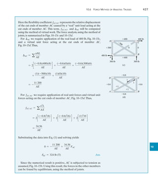
In a similar manner, for span BC we have
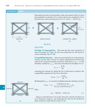
MBC = 2Ea
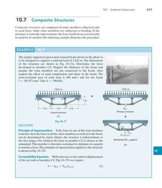
I
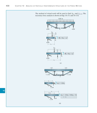
6
b[2uB + 0 - 3(0)] - 7.2 =
2EI
3
uB - 7.2 (3)
MCB = 2Ea
I
6
b[2(0) + uB - 3(0)] + 10.8 =
EI
3
uB + 10.8 (4)
EXAMPLE 11.1
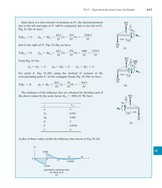
A B
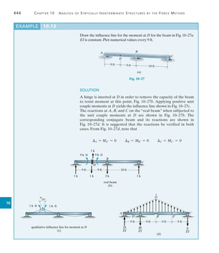
(a)
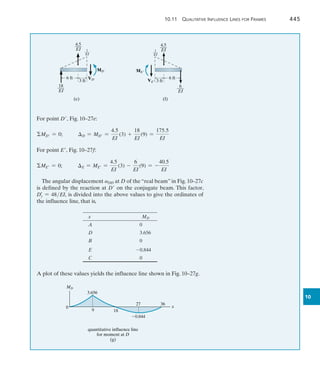
8 m 6 m
C
6 kN/m
A B
C
MBA
MBC
uB
uB
MCB
MAB
(b)
Fig. 11–10](https://image.slidesharecdn.com/structuralanalysis-hibbelerpdfdrive-220911133905-65f3c8d4/85/STRUCTURAL-ANALYSIS-NINTH-EDITION-R-C-HIBBELER-491-320.jpg)
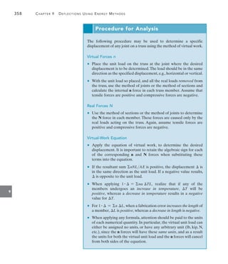
![472 Chapter 11 Displacement Method of Analysis: Slope-Deflection Equations
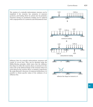
11
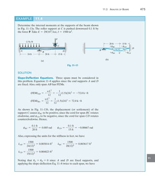
EXAMPLE 11.2
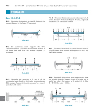
Draw the shear and moment diagrams for the beam shown in
Fig. 11–11a. EI is constant.
8 ft
24 ft
4 ft
2 k/ft
B
A
C
12 k
(a)
Fig. 11–11
SOLUTION
Slope-Deflection Equations. Two spans must be considered in this
problem. Equation 11–8 applies to span AB.We can use Eq. 11–10 for
span BC since the end C is on a roller. Using the formulas for the
FEMs tabulated on the inside back cover, we have
(FEM)AB = -
wL2
12
= -
1
12
(2)(24)2
= -96 k # ft
(FEM)BA =
wL2
12
=
1
12
(2)(24)2
= 96 k # ft
(FEM)BC = -
3PL
16
= -
3(12)(8)
16
= -18 k # ft
Note that (FEM)AB and (FEM)BC are negative since they act
counterclockwise on the beam at A and B, respectively.Also, since the
supports do not settle, cAB = cBC = 0. Applying Eq. 11–8 for span
AB and realizing that uA = 0, we have
MN = 2Ea
I
L
b(2uN + uF - 3c) + (FEM)N
MAB = 2Ea
I
24
b[2(0) + uB - 3(0)] - 96
MAB = 0.08333EIuB - 96 (1)
MBA = 2Ea
I
24
b[2uB + 0 - 3(0)] + 96
MBA = 0.1667EIuB + 96 (2)
Applying Eq. 11–10 with B as the near end and C as the far end, we have
MN = 3Ea
I
L
b(uN - c) + (FEM)N
MBC = 3Ea
I
8
b(uB - 0) - 18
MBC = 0.375EIuB - 18 (3)
Remember that Eq. 11–10 is not applied from C (near end) to B
(far end).](https://image.slidesharecdn.com/structuralanalysis-hibbelerpdfdrive-220911133905-65f3c8d4/85/STRUCTURAL-ANALYSIS-NINTH-EDITION-R-C-HIBBELER-493-320.jpg)
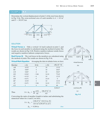
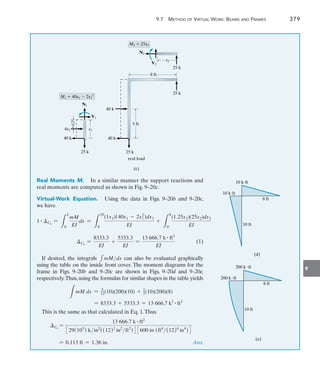
![474 Chapter 11 Displacement Method of Analysis: Slope-Deflection Equations
11
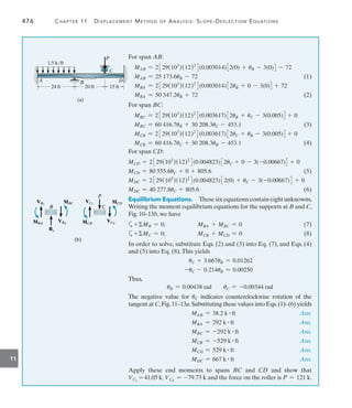
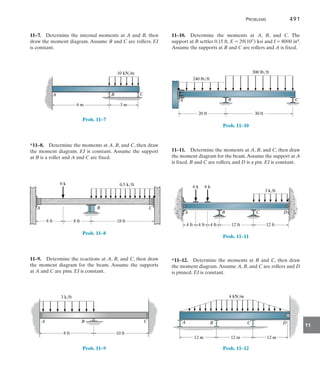
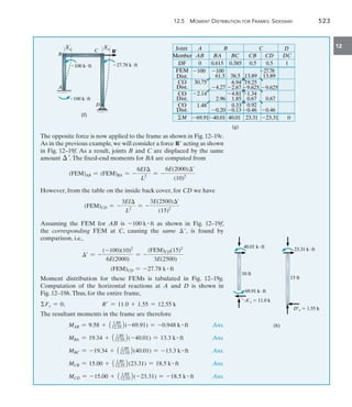
Determine the moment at A and B for the beam shown in Fig. 11–12a.
The support at B is displaced (settles) 80 mm. Take E = 200 GPa,
I = 5(106
) mm4
.
4 m 3 m
A
B
C
8 kN
(a)
Fig. 11–12
SOLUTION
Slope-Deflection Equations. Only one span (AB) must be
considered in this problem since the moment MBC due to the overhang
can be calculated from statics. Since there is no loading on span AB,
the FEMs are zero. As shown in Fig. 11–12b, the downward
displacement (settlement) of B causes the cord for span AB to rotate
clockwise.Thus,
cAB = cBA =
0.08 m
4
= 0.02 rad
The stiffness for AB is
k =
I
L
=
5(106
) mm4
(10-12
) m4
mm4
4 m
= 1.25(10-6
) m3
Applying the slope-deflection equation, Eq. 11–8, to span AB, with
uA = 0, we have
MN = 2Ea
I
L
b(2uN + uF - 3c) + (FEM)N
B
cBA
cAB
A
(b)
8000 N
8000 N
By
By
MBA
MBA 8000 N(3 m)
8000 N(3 m)
VBL
VBL
(c)
(c)
MAB = 2(200(109
) Nm2
)31.25(10-6
) m3
4[2(0) + uB - 3(0.02)] + 0(1)
MBA = 2(200(109
) Nm2
)31.25(10-6
) m3
4[2uB + 0 - 3(0.02)] + 0(2)
Equilibrium Equations. The free-body diagram of the beam at
support B is shown in Fig. 11–12c. Moment equilibrium requires
a+MB = 0; MBA - 8000 N(3 m) = 0
Substituting Eq. (2) into this equation yields
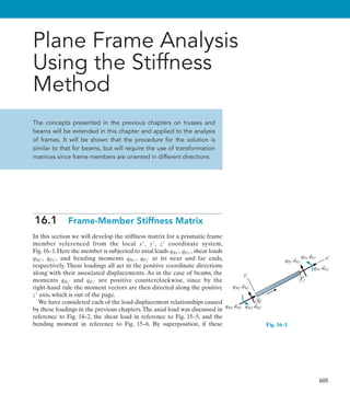
1(106
)uB - 30(103
) = 24(103
)
uB = 0.054 rad
Thus, from Eqs. (1) and (2),
MAB = -3.00 kN # m
MBA = 24.0 kN # m
EXAMPLE 11.3](https://image.slidesharecdn.com/structuralanalysis-hibbelerpdfdrive-220911133905-65f3c8d4/85/STRUCTURAL-ANALYSIS-NINTH-EDITION-R-C-HIBBELER-495-320.jpg)
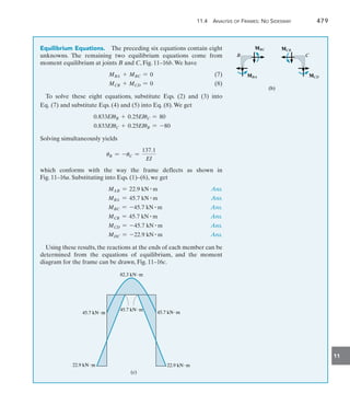
![478 Chapter 11 Displacement Method of Analysis: Slope-Deflection Equations
11
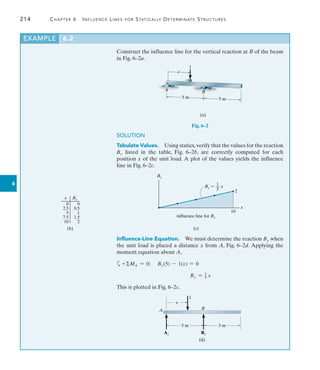
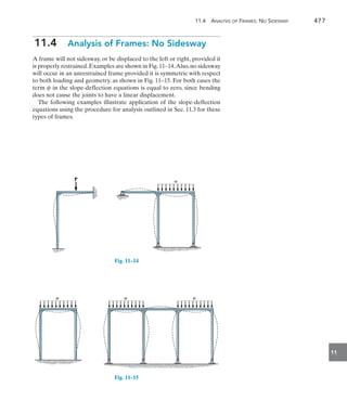
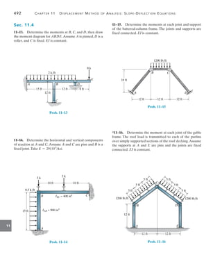
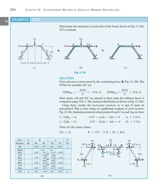
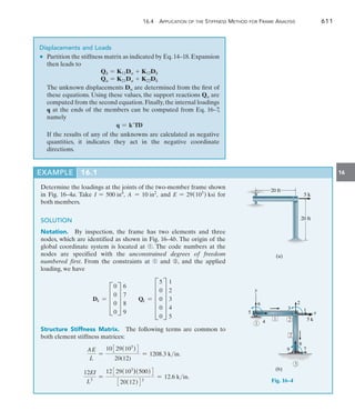
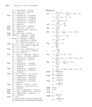
Determine the moments at each joint of the frame shown in
Fig. 11–16a. EI is constant.
SOLUTION
Slope-Deflection Equations. Three spans must be considered in
this problem: AB, BC, and CD. Since the spans are fixed supported at
A and D, Eq. 11–8 applies for the solution.
From the table on the inside back cover, the FEMs for BC are
(FEM)BC = -
5wL2
96
= -
5(24)(8)2
96
= -80 kN # m
(FEM)CB =
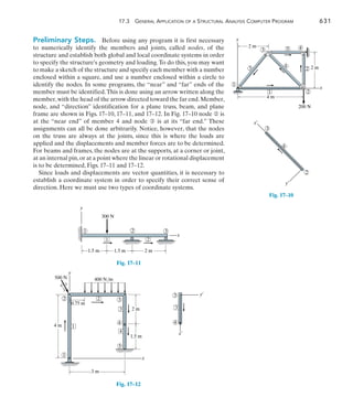
5wL2
96
=
5(24)(8)2
96
= 80 kN # m
Note that uA = uD = 0 and cAB = cBC = cCD = 0, since no sidesway
will occur.
Applying Eq. 11–8, we have
MN = 2Ek(2uN + uF - 3c) + (FEM)N
MAB = 2Ea
I
12
b[2(0) + uB - 3(0)] + 0
MAB = 0.1667EIuB(1)
MBA = 2Ea
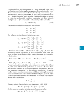
I
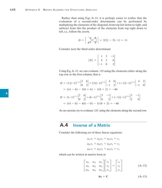
12
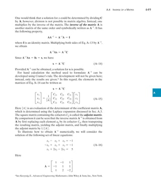
b[2uB + 0 - 3(0)] + 0
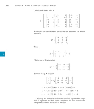
MBA = 0.333EIuB(2)
MBC = 2Ea
I
8
b[2uB + uC - 3(0)] - 80
MBC = 0.5EIuB + 0.25EIuC - 80(3)
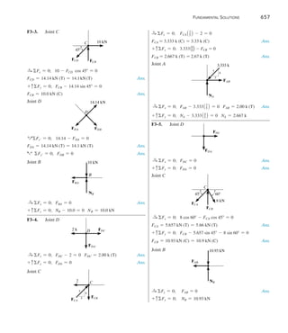
MCB = 2Ea
I
8
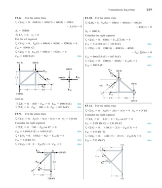
b[2uC + uB - 3(0)] + 80
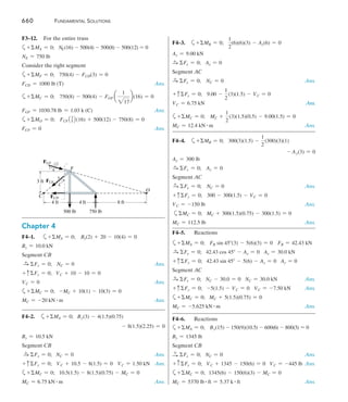
MCB = 0.5EIuC + 0.25EIuB + 80(4)
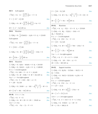
MCD = 2Ea
I
12
b[2uC + 0 - 3(0)] + 0
MCD = 0.333EIuC(5)
MDC = 2Ea
I
12
b[2(0) + uC - 3(0)] + 0
MDC = 0.1667EIuC(6)
B
24 kN/m
C
A
D
8 m
12 m
(a)
Fig. 11–16
EXAMPLE 11.5](https://image.slidesharecdn.com/structuralanalysis-hibbelerpdfdrive-220911133905-65f3c8d4/85/STRUCTURAL-ANALYSIS-NINTH-EDITION-R-C-HIBBELER-499-320.jpg)
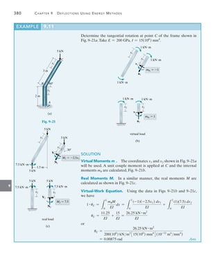
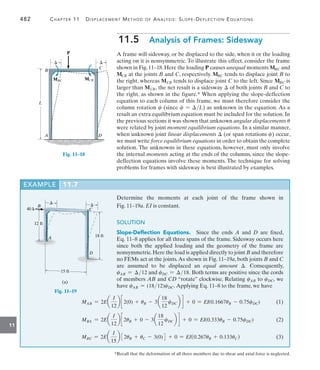
![480 Chapter 11 Displacement Method of Analysis: Slope-Deflection Equations
11
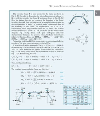
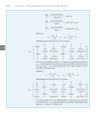
Determine the internal moments at each joint of the frame shown in
Fig. 11–17a. The moment of inertia for each member is given in the
figure.Take E = 29(103
) ksi.
3 k/ft
6 k
8 ft
8 ft
15 ft
B
A
C
D
E
400 in4
200 in4
800 in4
650 in4
(a)
12 ft
Fig. 11–17
SOLUTION
Slope-Deflection Equations. Four spans must be considered in this
problem. Equation 11–8 applies to spans AB and BC, and Eq. 11–10
will be applied to CD and CE, because the ends at D and E are pinned.
Computing the member stiffnesses, we have
kAB =
400
15(12)4
= 0.001286 ft3
kCD =
200
15(12)4
= 0.000643 ft3
kBC =
800
16(12)4
= 0.002411 ft3
kCE =
650
12(12)4
= 0.002612 ft3
The FEMs due to the loadings are
(FEM)BC = -
PL
8
= -
6(16)
8
= -12 k # ft
(FEM)CB =
PL
8
=
6(16)
8
= 12 k # ft
(FEM)CE = -
wL2
8
= -
3(12)2
8
= -54 k # ft
Applying Eqs. 11–8 and 11–10 to the frame and noting that uA = 0,
cAB = cBC = cCD = cCE = 0 since no sidesway occurs, we have
MN = 2Ek(2uN + uF - 3c) + (FEM)N
MAB = 2329(103
)(12)2
4(0.001286)[2(0) + uB - 3(0)] + 0
MAB = 10740.7uB(1)
EXAMPLE 11.6](https://image.slidesharecdn.com/structuralanalysis-hibbelerpdfdrive-220911133905-65f3c8d4/85/STRUCTURAL-ANALYSIS-NINTH-EDITION-R-C-HIBBELER-501-320.jpg)
![11.4 Analysis of Frames: No Sidesway 481
11
MBA = 2329(103
)(12)2
4(0.001286)[2uB + 0 - 3(0)] + 0
MBA = 21 481.5uB(2)
MBC = 2329(103
)(12)2
4(0.002411)[2uB + uC - 3(0)] - 12
MBC = 40 277.8uB + 20 138.9uC - 12(3)
MCB = 2329(103
)(12)2
4(0.002411)[2uC + uB - 3(0)] + 12
MCB = 20 138.9uB + 40 277.8uC + 12(4)
MN = 3Ek(uN - c) + (FEM)N
MCD = 3329(103
)(12)2
4(0.000643)[uC - 0] + 0(5)
MCD = 8055.6uC
MCE = 3329(103
)(12)2
4(0.002612)[uC - 0] - 54
MCE = 32 725.7uC - 54(6)
Equations of Equilibrium. These six equations contain eight
unknowns. Two moment equilibrium equations can be written for
joints B and C, Fig. 11–17b.We have
MBA + MBC = 0(7)
MCB + MCD + MCE = 0(8)
In order to solve,substitute Eqs.(2) and (3) into Eq.(7),and Eqs. (4)–(6)
into Eq. (8).This gives
61 759.3uB + 20 138.9uC = 12
20 138.9uB + 81 059.0uC = 42
Solving these equations simultaneously yields
uB = 2.758(10-5
) rad uC = 5.113(10-4
) rad
These values, being clockwise, tend to distort the frame as shown in
Fig.11–17a.Substituting these values into Eqs.(1)–(6) and solving,we get
MAB = 0.296 k # ft Ans.
MBA = 0.592 k # ft Ans.
MBC = -0.592 k # ft Ans.
MCB = 33.1 k # ft Ans.
MCD = 4.12 k # ft Ans.
MCE = -37.3 k # ft Ans.
MBC
MBC
MBA
MBA
B
B C
C
MCE
MCE
MCD
MCD
MCB
MCB
(b)
(b)](https://image.slidesharecdn.com/structuralanalysis-hibbelerpdfdrive-220911133905-65f3c8d4/85/STRUCTURAL-ANALYSIS-NINTH-EDITION-R-C-HIBBELER-502-320.jpg)
![11.5 Analysis of Frames: Sidesway 483
11
MCB = 2Ea
I
15
b[2uC + uB - 3(0)] + 0 = EI(0.267uC + 0.133uB)
MCD = 2Ea
I
18
b[2uC + 0 - 3cDC] + 0 = EI(0.222uC - 0.333cDC)
MDC = 2Ea
I
18
b[2(0) + uC - 3cDC] + 0 = EI(0.111uC - 0.333cDC)
Equations of Equilibrium. The six equations contain nine
unknowns. Two moment equilibrium equations for joints B and C,
Fig. 11–19b, can be written, namely,
MBA + MBC = 0
MCB + MCD = 0
Since a horizontal displacement occurs, we will consider summing
forces on the entire frame in the x direction.This yields
+
S Fx = 0; 40 - VA - VD = 0
The horizontal reactions or column shears VA and VD can be related
to the internal moments by considering the free-body diagram of each
column separately, Fig. 11–19c.We have
MB = 0; VA = -
MAB + MBA
12
MC = 0; VD = -
MDC + MCD
18
Thus,
40 +
MAB + MBA
12
+
MDC + MCD
18
= 0
In order to solve, substitute Eqs. (2) and (3) into Eq. (7), Eqs. (4)
and (5) into Eq. (8), and Eqs. (1), (2), (5), (6) into Eq. (9).This yields
0.6uB + 0.133uC - 0.75cDC = 0
0.133uB + 0.489uC - 0.333cDC = 0
0.5uB + 0.222uC - 1.944cDC = -
480
EI
Solving simultaneously, we have
EIuB = 438.81 EIuC = 136.18 EIcDC = 375.26
Finally, using these results and solving Eqs. (1)–(6) yields
MAB = -208 k # ft Ans.
MBA = -135 k # ft Ans.
MBC = 135 k # ft Ans.
MCB = 94.8 k # ft Ans.
MCD = -94.8 k # ft Ans.
MDC = -110 k # ft Ans.
B
B
MBC
MBC
MBA
MBA
C
C
MCB
MCB
MCD
MCD
(b)
(b)
40 k
40 k
B
MBA
MAB
VA
12 ft
C
MCD
18 ft
MDC
VD
(c)
(4)
(5)
(6)
(7)
(8)
(9)](https://image.slidesharecdn.com/structuralanalysis-hibbelerpdfdrive-220911133905-65f3c8d4/85/STRUCTURAL-ANALYSIS-NINTH-EDITION-R-C-HIBBELER-504-320.jpg)
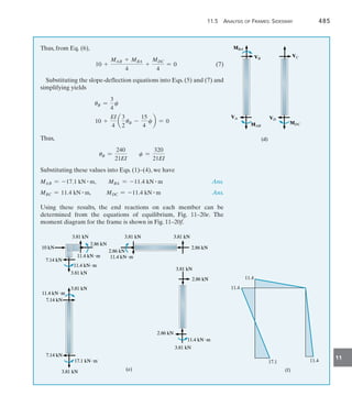
![484 Chapter 11 Displacement Method of Analysis: Slope-Deflection Equations
11
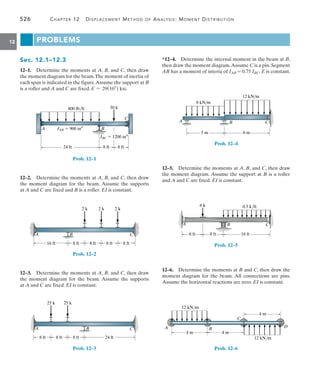
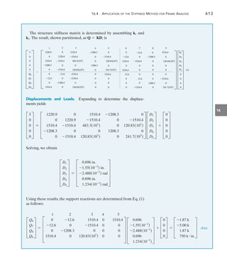
Determine the moments at each joint of the frame shown in
Fig. 11–20a.The supports at A and D are fixed and joint C is assumed
pin connected. EI is constant for each member.
SOLUTION
Slope-Deflection Equations. We will apply Eq. 11–8 to member
AB since it is fixed connected at both ends. Equation 11–10 can be
applied from B to C and from D to C since the pin at C supports zero
moment. As shown by the deflection diagram, Fig. 11–20b, there is an
unknown linear displacement of the frame and unknown angular
displacement uB at joint B.* Due to , the cord members AB and CD
rotate clockwise, c = cAB = cDC = 4. Realizing that uA = uD = 0
and that there are no FEMs for the members, we have
MN = 2Ea
I
L
b(2uN + uF - 3c) + (FEM)N
MAB = 2Ea
I
4
b[2(0) + uB - 3c] + 0(1)
MBA = 2Ea
I
4
b(2uB + 0 - 3c) + 0(2)
MN = 3Ea
I
L
b(uN - c) + (FEM)N
MBC = 3Ea
I
3
b(uB - 0) + 0(3)
MDC = 3Ea
I
4
b(0 - c) + 0(4)
Equilibrium Equations.
Moment equilibrium of joint B,
Fig. 11–20c, requires
MBA + MBC = 0(5)
If forces are summed for the entire frame in the horizontal direction,
we have
+
S Fx = 0; 10 - VA - VD = 0(6)
As shown on the free-body diagram of each column,Fig.11–20d,we have
MB = 0; VA = -
MAB + MBA
4
MC = 0; VD = -
MDC
4
3 m
10 kN
4 m
A
B C
D
(a)
Fig. 11–20
uB
uB uCB
uCD
cCD
cAB
C
B
A D
(b)
MBC
MBC
10 kN
10 kN
MBA
MBA
(c)
(c)
*The angular displacements uCB and uCD at joint C (pin) are not included in the analysis
since Eq. 11–10 is to be used.
EXAMPLE 11.8](https://image.slidesharecdn.com/structuralanalysis-hibbelerpdfdrive-220911133905-65f3c8d4/85/STRUCTURAL-ANALYSIS-NINTH-EDITION-R-C-HIBBELER-505-320.jpg)
![486 Chapter 11 Displacement Method of Analysis: Slope-Deflection Equations
11
Explain how the moments in each joint of the two-story frame shown
in Fig. 11–21a are determined. EI is constant.
SOLUTION
Slope-Deflection Equation. Since the supports at A and F are
fixed, Eq. 11–8 applies for all six spans of the frame. No FEMs have to
be calculated, since the applied loading acts at the joints. Here the
loading displaces joints B and E an amount 1, and C and D an
amount 1 + 2. As a result, members AB and FE undergo rotations
of c1 = 15 and BC and ED undergo rotations of c2 = 25.
Applying Eq. 11–8 to the frame yields
MAB = 2Ea
I
5
b[2(0) + uB - 3c1] + 0(1)
MBA = 2Ea
I
5
b[2uB + 0 - 3c1] + 0(2)
MBC = 2Ea
I
5
b[2uB + uC - 3c2] + 0(3)
MCB = 2Ea
I
5
b[2uC + uB - 3c2] + 0(4)
MCD = 2Ea
I
7
b[2uC + uD - 3(0)] + 0(5)
MDC = 2Ea
I
7
b[2uD + uC - 3(0)] + 0(6)
MBE = 2Ea
I
7
b[2uB + uE - 3(0)] + 0(7)
MEB = 2Ea
I
7
b[2uE + uB - 3(0)] + 0(8)
MED = 2Ea
I
5
b[2uE + uD - 3c2] + 0(9)
MDE = 2Ea
I
5
b[2uD + uE - 3c2] + 0(10)
MFE = 2Ea
I
5
b[2(0) + uE - 3c1] + 0(11)
MEF = 2Ea
I
5
b[2uE + 0 - 3c1] + 0(12)
These 12 equations contain 18 unknowns.
A
B
D
E
C
F
40 kN
80 kN
5 m
(a)
5 m
1
1
1 2 1 2
7 m
Fig. 11–21
EXAMPLE 11.9](https://image.slidesharecdn.com/structuralanalysis-hibbelerpdfdrive-220911133905-65f3c8d4/85/STRUCTURAL-ANALYSIS-NINTH-EDITION-R-C-HIBBELER-507-320.jpg)
![11.5 Analysis of Frames: Sidesway 489
11
MAB = 2Ea
I
10
b[2(0) + uB - 3c1] + 0(1)
MBA = 2Ea
I
10
b[2uB + 0 - 3c1] + 0(2)
MBC = 2Ea
I
12
b[2uB + uC - 3(-0.417c1)] - 24(3)
MCB = 2Ea
I
12
b[2uC + uB - 3(-0.417c1)] + 24(4)
MCD = 2Ea
I
20
b[2uC + 0 - 3(0.433c1)] + 0(5)
MDC = 2Ea
I
20
b[2(0) + uC - 3(0.433c1)] + 0(6)
These six equations contain nine unknowns.
Equations of Equilibrium. Moment equilibrium at joints B and C
yields
MBA + MBC = 0(7)
MCD + MCB = 0(8)
The necessary third equilibrium equation can be obtained by summing
moments about point O on the entire frame, Fig. 11–22d. This
eliminates the unknown normal forces NA and ND, and therefore
c+MO = 0;
MAB + MDC - a
MAB + MBA
10
b(34) - a
MDC + MCD
20
b(40.78) - 24(6) = 0
-2.4MAB - 3.4MBA - 2.04MCD - 1.04MDC - 144 = 0(9)
Substituting Eqs. (2) and (3) into Eq. (7), Eqs. (4) and (5) into Eq. (8),
and Eqs. (1), (2), (5), and (6) into Eq. (9) yields
0.733uB + 0.167uC - 0.392c1 =
24
EI
0.167uB + 0.533uC + 0.0784c1 = -
24
EI
-1.840uB - 0.512uC + 3.880c1 =
144
EI
Solving these equations simultaneously yields
EIuB = 87.67 EIuC = -82.3 EIc1 = 67.83
Substituting these values into Eqs. (1)–(6), we have
MAB = -23.2 k # ft MBC = 5.63 k # ft MCD = -25.3 k # ft Ans.
MBA = -5.63 k # ft MCB = 25.3 k # ft MDC = -17.0 k # ft Ans.
10 ft
10 ft
24 ft
24 ft
30
30
20.78 ft
20.78 ft
24 k
24 k
20 ft
20 ft
ND
ND
MDC
MDC
MAB MBA
VA ___________
10
MAB MBA
VA ___________
10
MDC MCD
VD ___________
20
MDC MCD
VD ___________
20
6 ft
6 ft 6 ft
6 ft
NA
NA
MAB
MAB
(d)
(d)
O
O](https://image.slidesharecdn.com/structuralanalysis-hibbelerpdfdrive-220911133905-65f3c8d4/85/STRUCTURAL-ANALYSIS-NINTH-EDITION-R-C-HIBBELER-510-320.jpg)


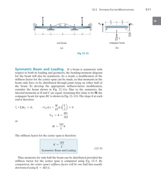

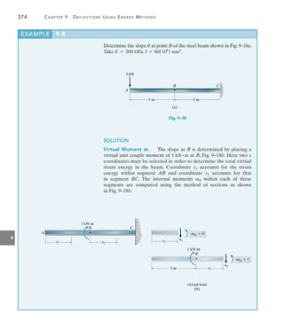
![542 Chapter 13 Beams and Frames Having Nonprismatic Members
13
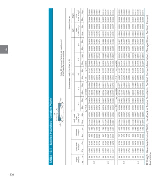
Determine the internal moments at the supports of the beam shown
in Fig. 13–9a.The beam has a thickness of 1 ft and E is constant.
3 ft
30 k
2 k/ft
5 ft
C
25 ft
5 ft 15 ft 5 ft 5 ft
10 ft
(a)
5 ft
4 ft
A B
2 ft
4 ft
2 ft
Fig. 13–9
SOLUTION
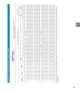
Since the haunches are parabolic, we will use Table 13.2 to obtain the
moment-distribution properties of the beam.
Span AB
aA = aB =
5
25
= 0.2 rA = rB =
4 - 2
2
= 1.0
Entering Table 13.2 with these ratios, we find
CAB = CBA = 0.619
kAB = kBA = 6.41
Using Eqs. 13–2,
KAB = KBA =
kEIC
L
=
6.41E1 1
122(1)(2)3
25
= 0.171E
Since the far end of span BA is pinned, we will modify the stiffness
factor of BA using Eq. 13–3.We have
KBA
=
= KBA (1 - CABCBA ) = 0.171E[1 - 0.619(0.619)] = 0.105E
Uniform load,Table 13.2,
(FEM)AB = -(0.0956)(2)(25)2
= -119.50 k # ft
(FEM)BA = 119.50 k # ft
EXAMPLE 13.1](https://image.slidesharecdn.com/structuralanalysis-hibbelerpdfdrive-220911133905-65f3c8d4/85/STRUCTURAL-ANALYSIS-NINTH-EDITION-R-C-HIBBELER-563-320.jpg)


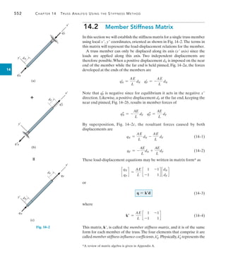
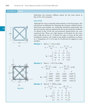
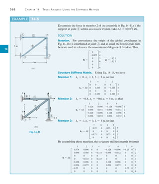
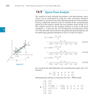
![562 Chapter 14 Truss Analysis Using the Stiffness Method
14
14.6
Application of the Stiffness Method
for Truss Analysis
Once the structure stiffness matrix is formed,the global force components Q
acting on the truss can then be related to its global displacements D using
Q = KD(14–17)
This equation is referred to as the structure stiffness equation. Since we
have always assigned the lowest code numbers to identify the uncon
strained degrees of freedom,this will allow us now to partition this equation
in the following form*:
(14–18)
Here
Qk, Dk =
known external loads and displacements; the loads here exist
on the truss as part of the problem, and the displacements are
generally specified as zero due to support constraints such as
pins or rollers.
Qu, Du =
unknown loads and displacements; the loads here represent
the unknown support reactions, and the displacements are at
joints where motion is unconstrained in a particular direction.
K =
structure stiffness matrix,which is partitioned to be compatible
with the partitioning of Q and D.
Expanding Eq. 14–18 yields
Qk = K11Du + K12Dk(14–19)
Qu = K21Du + K22Dk(14–20)
Most often Dk = 0 since the supports are not displaced. Provided this is
the case, Eq. 14–19 becomes
Qk = K11Du
Since the elements in the partitioned matrix K11 represent the total
resistance at a truss joint to a unit displacement in either the x or y
direction, then the above equation symbolizes the collection of all the
force equilibrium equations applied to the joints where the external loads
are zero or have a known value (Qk). Solving for Du, we have
Du = [K11]-1
Qk (14–21)
From this equation we can obtain a direct solution for all the unknown
joint displacements; then using Eq. 14–20 with Dk = 0 yields
Qu = K21Du(14–22)
from which the unknown support reactions can be determined. The
member forces can be determined using Eq. 14–13, namely
q = kTD
c
Qk
Qu
d = c
K11 K12
K21 K22
d c
Du
Dk
d
*This partitioning scheme will become obvious in the numerical examples that follow.](https://image.slidesharecdn.com/structuralanalysis-hibbelerpdfdrive-220911133905-65f3c8d4/85/STRUCTURAL-ANALYSIS-NINTH-EDITION-R-C-HIBBELER-583-320.jpg)
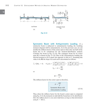
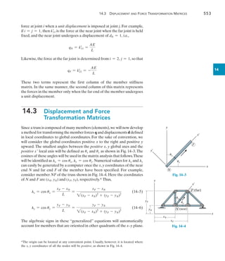
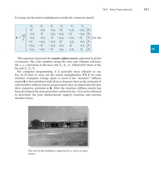
![14.6 Application of the Stiffness Method for Truss Analysis 563
14
Expanding this equation yields
c
qN
qF
d =
AE
L
c
1 -1
-1 1
d c
lx ly 0 0
0 0 lx ly
d D
DNx
DNy
DFx
DFy
T
Since qN = -qF for equilibrium,only one of the forces has to be found.Here
we will determine qF, the one that exerts tension in the member, Fig. 14–2c.
(14–23)
In particular, if the computed result using this equation is negative, the
member is then in compression.
Procedure for Analysis
The following method provides a means for determining the unknown
displacements and support reactions for a truss using the stiffness method.
Notation
• Establish the x,y global coordinate system.The origin is usually located
at the joint for which the coordinates for all the other joints are positive.
• Identify each joint and member numerically,and arbitrarily specify the
near and far ends of each member symbolically by directing an arrow
along the member with the head directed towards the far end.
• Specify the two code numbers at each joint,using the lowest numbers
to identify unconstrained degrees of freedom, followed by the highest
numbers to identify the constrained degrees of freedom.
• From the problem, establish Dk and Qk.
Structure Stiffness Matrix
• For each member determine x and y and the member stiffness
matrix using Eq. 14–16.
• Assemble these matrices to form the stiffness matrix for the entire
truss as explained in Sec. 14.5. As a partial check of the calculations,
the member and structure stiffness matrices should be symmetric.
Displacements and Loads
• Partition the structure stiffness matrix as indicated by Eq. 14–18.
• Determine the unknown joint displacements Du using Eq. 14–21, the
support reactions Qu using Eq. 14–22, and each member force qF
using Eq. 14–23.
qF =
AE
L
[-lx -ly lx ly]D
DNx
DNy
DFx
DFy
T](https://image.slidesharecdn.com/structuralanalysis-hibbelerpdfdrive-220911133905-65f3c8d4/85/STRUCTURAL-ANALYSIS-NINTH-EDITION-R-C-HIBBELER-584-320.jpg)
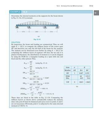
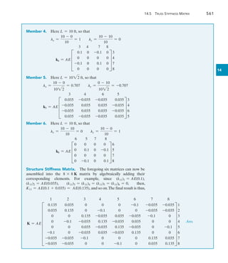
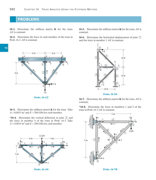
![14.6 Application of the Stiffness Method for Truss Analysis 565
14
By inspection of Fig. 14–9b, one would indeed expect a rightward and
downward displacement to occur at joint 2 as indicated by the
positive and negative signs of these answers.
Using these results, the support reactions are now obtained from
Eq. (1), written in the form of Eq. 14–20 (or Eq. 14–22) as
D
Q3
Q4
Q5
Q6
T = AE D
-0.333 0
0 0
-0.072 -0.096
-0.096 -0.128
T
1
AE
c
4.505
-19.003
d + D
0
0
0
0
T
Expanding and solving for the reactions,
Q3 = -0.333(4.505) = -1.5 k
Q4 = 0
Q5 = -0.072(4.505) - 0.096(-19.003) = 1.5 k
Q6 = -0.096(4.505) - 0.128(-19.003) = 2.0 k
The force in each member is found from Eq. 14–23. Using the data
for lx and ly in Example 14.1, we have
Member 1: lx = 1, ly = 0, L = 3 ft
q1 =
AE
3
1 2 3 4
3 -1 0 1 04
1
AE
D
4.505
-19.003
0
0
T
1
2
3
4
=
1
3
[-4.505] = -1.5 k Ans.
Member 2: lx = 0.6, ly = 0.8, L = 5 ft
q2 =
AE
5
1 2 5 6
3 -0.6 -0.8 0.6 0.84
1
AE
D
4.505
-19.003
0
0
T
1
2
5
6
=
1
5
[-0.6(4.505) - 0.8(-19.003)] = 2.5 k Ans.
These answers can of course be verified by equilibrium, applied at
joint 2 .
2 3
1
6
5
2
1
4
3
1
2
x
y
(b)
2 k](https://image.slidesharecdn.com/structuralanalysis-hibbelerpdfdrive-220911133905-65f3c8d4/85/STRUCTURAL-ANALYSIS-NINTH-EDITION-R-C-HIBBELER-586-320.jpg)
![14.6 Application of the Stiffness Method for Truss Analysis 567
14
Expanding and solving the equations for the displacements yields
E
D1
D2
D3
D4
D5
U =
1
AE
E
17.94
-69.20
-2.06
-87.14
-22.06
U
Developing Eq. 14–20 from Eq. (1) using the calculated results, we
have
C
Q6
Q7
Q8
S = AE C
-0.1 0 -0.035 0.035 -0.035
-0.035 -0.035 -0.1 0 0
-0.035 -0.035 0 0 -0.1
S
1
AE
E
17.94
-69.20
-2.06
-87.14
-22.06
U + C
0
0
0
S
Expanding and computing the support reactions yields
Q6 = -4.0 k Ans.
Q7 = 2.0 k Ans.
Q8 = 4.0 k Ans.
The negative sign for Q6 indicates that the rocker support reaction
acts in the negative x direction. The force in member 2 is found from
Eq. 14–23, where from Example 14.2, lx = 0.707, ly = 0.707,
L = 1012 ft. Thus,
q2 =
AE
1022
[-0.707 -0.707 0.707 0.707]
1
AE
D
17.94
-69.20
0
0
T
= 2.56 k Ans.](https://image.slidesharecdn.com/structuralanalysis-hibbelerpdfdrive-220911133905-65f3c8d4/85/STRUCTURAL-ANALYSIS-NINTH-EDITION-R-C-HIBBELER-588-320.jpg)
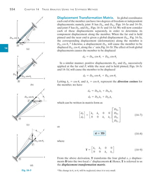
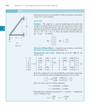
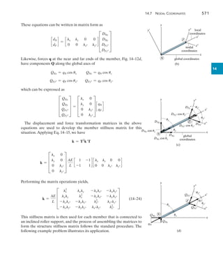
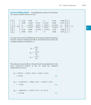
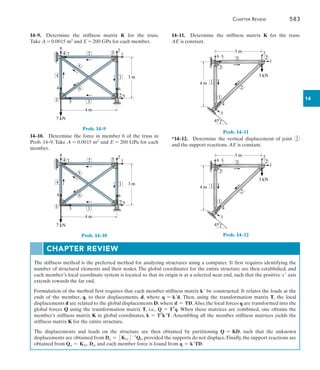
![14.6 Application of the Stiffness Method for Truss Analysis 569
14
2
11.1 kN
8.34 kN
13.9 kN
3
4
5
(c)
Displacements and Loads. Here Q = KD yields
H
0
0
Q3
Q4
Q5
Q6
Q7
Q8
X = AE H
0.378 0.096 0 0 -0.128 -0.096 -0.25 0
0.096 0.405 0 -0.333 -0.096 -0.072 0 0
0 0 0 0 0 0 0 0
0 -0.333 0 0.333 0 0 0 0
-0.128 -0.096 0 0 0.128 0.096 0 0
-0.096 -0.072 0 0 0.096 0.072 0 0
-0.25 0 0 0 0 0 0.25 0
0 0 0 0 0 0 0 0
X H
D1
D2
0
-0.025
0
0
0
0
X
Developing the solution for the displacements, Eq. 14–19, we have
c
0
0
d = AE c
0.378 0.096
0.096 0.405
d c
D1
D2
d + AE c
0 0 -0.128 -0.096 -0.25 0
0 -0.333 -0.096 -0.072 0 0
d F
0
-0.025
0
0
0
0
V
which yields
0 = AE3(0.378D1 + 0.096D2) + 04
0 = AE3(0.096D1 + 0.405D2) + 0.008334
Solving these equations simultaneously gives
D1 = 0.00556 m
D2 = -0.021875 m
Although the support reactions do not have to be calculated, if needed
they can be found from the expansion defined by Eq. 14–20. Using
Eq. 14–23 to determine the force in member 2 yields
Member 2: lx = -0.8, ly = -0.6, L = 5 m, AE = 8(103
) kN,
so that
q2 =
8(103
)
5
[0.8 0.6 -0.8 -0.6]D
0.00556
-0.021875
0
0
T
=
8(103
)
5
(0.00444 - 0.0131) = -13.9 kN Ans.
Using the same procedure, show that the force in member 1 is
q1 = 8.34 kN and in member 3, q3 = 11.1 kN. The results are shown
on the free-body diagram of joint 2 ,Fig.14–11c,which can be checked
to be in equilibrium.](https://image.slidesharecdn.com/structuralanalysis-hibbelerpdfdrive-220911133905-65f3c8d4/85/STRUCTURAL-ANALYSIS-NINTH-EDITION-R-C-HIBBELER-590-320.jpg)
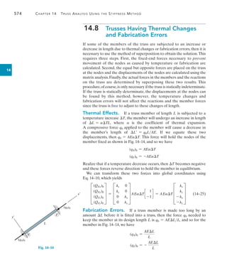
![14.8 Trusses Having Thermal Changes and Fabrication Errors 575
14
If the member is originally too short, then L becomes negative and
these forces will reverse.
In global coordinates, these forces are
D
(QNx)0
(QNy)0
(QFx)0
(QFy)0
T =
AEL
L
D
lx
ly
-lx
-ly
T (14–26)
Matrix Analysis. In the general case, with the truss subjected to
applied forces, temperature changes, and fabrication errors, the initial
force-displacement relationship for the truss then becomes
Q = KD + Q0 (14–27)
Here Q0 is a column matrix for the entire truss of the initial fixed-end
forces caused by the temperature changes and fabrication errors of the
members defined in Eqs. 14–25 and 14–26.We can partition this equation
in the following form
c
Qk
Qu
d = c
K11 K12
K21 K22
d c
Du
Dk
d + c
(Qk)0
(Qu)0
d
Carrying out the multiplication, we obtain
Qk = K11Du + K12Dk + (Qk)0 (14–28)
Qu = K21Du + K22Dk + (Qu)0 (14–29)
According to the superposition procedure described above, the unknown
displacements Du are determined from the first equation by subtracting
K12Dk and (Qk)0 from both sides and then solving for Du. This yields
Du = K11
-1
(Qk - K12Dk - (Qk)0)
Once these nodal displacements are obtained,the member forces are then
determined by superposition, i.e.,
q = kTD + q0
If this equation is expanded to determine the force at the far end of the
member, we obtain
qF =
AE
L
[-lx -ly lx ly ]D
DNx
DNy
DFx
DFy
T + (qF)0 (14–30)
This result is similar to Eq. 14–23, except here we have the additional
term (qF)0 which represents the initial fixed-end member force due to
temperature changes and/or fabrication error as defined previously.
Realize that if the computed result from this equation is negative, the
member will be in compression.
The following two examples illustrate application of this procedure.](https://image.slidesharecdn.com/structuralanalysis-hibbelerpdfdrive-220911133905-65f3c8d4/85/STRUCTURAL-ANALYSIS-NINTH-EDITION-R-C-HIBBELER-596-320.jpg)
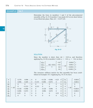
![14.8 Trusses Having Thermal Changes and Fabrication Errors 577
14
Partitioning the matrices as shown and carrying out the multiplication
to obtain the equations for the unknown displacements yields
c
0
0
d = AE c
0.378 0.096
0.096 0.405
d c
D1
D2
d + AE c
0 0 -0.128 -0.096 -0.25 0
0 -0.333 -0.096 -0.072 0 0
d F
0
0
0
0
0
0
V + AE c
0.0016
0.0012
d
which gives
0 = AE [0.378D1 + 0.096D2] + AE[0] + AE[0.0016]
0 = AE [0.096D1 + 0.405D2] + AE[0] + AE[0.0012]
Solving these equations simultaneously,
D1 = -0.003704 m
D2 = -0.002084 m
Although not needed,the reactions Q can be found from the expansion
of Eq. (1) following the format of Eq. 14–29.
In order to determine the force in members 1 and 2 we must apply
Eq. 14–30, in which case we have
Member 1. lx = 0, ly = 1, L = 3 m, AE = 8(103
) kN, so that
q1 =
8(103
)
3
[0 -1 0 1]D
0
0
-0.003704
-0.002084
T + [0]
q1 = -5.56 kN Ans.
Member 2. lx = -0.8, ly = -0.6, L = 5 m, AE = 8(103
) kN, so
q2 =
8(103
)
5
[0.8 0.6 -0.8 -0.6]D
-0.003704
-0.002084
0
0
T -
8(103
) (-0.01)
5
q2 = 9.26 kN Ans.](https://image.slidesharecdn.com/structuralanalysis-hibbelerpdfdrive-220911133905-65f3c8d4/85/STRUCTURAL-ANALYSIS-NINTH-EDITION-R-C-HIBBELER-598-320.jpg)
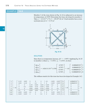
![14.8 Trusses Having Thermal Changes and Fabrication Errors 579
14
Expanding to determine the equations of the unknown displacements,
and solving these equations simultaneously, yields
D1 = -0.002027 ft
D2 = -0.01187 ft
D3 = -0.002027 ft
D4 = -0.009848 ft
D5 = -0.002027 ft
Using Eq. 14–30 to determine the force in member 2, we have
q2 =
0.75329(106
)4
1022
[-0.707 -0.707 0.707 0.707]D
-0.002027
-0.01187
0
0
T - 0.75329(106
)4 36.5(10-6
)4(150)
= -6093 lb = -6.09 k Ans.
Note that the temperature increase of member 2 will not cause any
reactions on the truss since externally the truss is statically determinate.
To show this, consider the matrix expansion of Eq. (1) for determining
the reactions. Using the results for the displacements, we have
Q6 = AE[-0.1(-0.002027) + 0 - 0.035(-0.002027)
+ 0.035(-0.009848) - 0.035(-0.002027)] + AE[0] = 0
Q7 = AE[-0.035(-0.002027) - 0.035(-0.01187)
- 0.1(-0.002027) + 0 + 0] + AE[-0.000689325] = 0
Q8 = AE[-0.035(-0.002027) - 0.035(-0.01187) + 0
+ 0 - 0.1(-0.002027)] + AE[-0.000689325] = 0](https://image.slidesharecdn.com/structuralanalysis-hibbelerpdfdrive-220911133905-65f3c8d4/85/STRUCTURAL-ANALYSIS-NINTH-EDITION-R-C-HIBBELER-600-320.jpg)

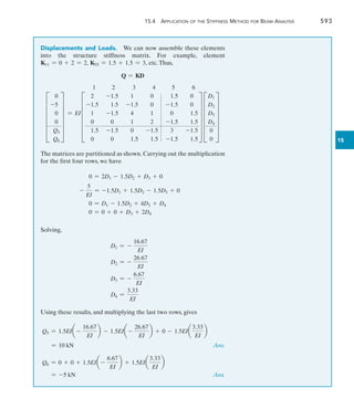
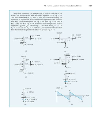
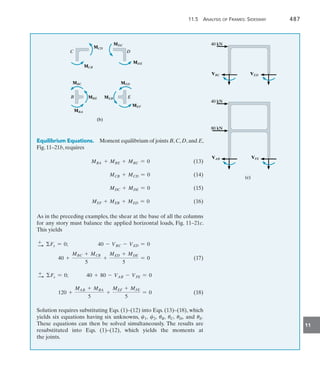
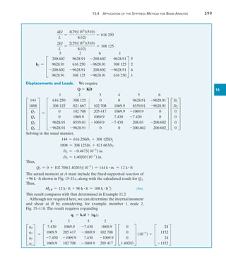
![15.4 Application of the Stiffness Method for Beam Analysis 597
15
k1 = EI
6 3 5 2
D
1.5 1.5 -1.5 1.5
1.5 2 -1.5 1
-1.5 -1.5 1.5 -1.5
1.5 1 -1.5 2
T
6
3
5
2
k2 = EI
5 2 4 1
D
1.5 1.5 -1.5 1.5
1.5 2 -1.5 1
-1.5 -1.5 1.5 -1.5
1.5 1 -1.5 2
T
5
2
4
1
Displacements and Loads. Assembling the structure stiffness
matrix and writing the stiffness equation for the structure, yields
F
4
0
-4
Q4
Q5
Q6
V
= EI
1 2 3 4 5 6
F
2 1 0 -1.5 1.5 0
1 4 1 -1.5 0 1.5
0 1 2 0 -1.5 1.5
-1.5 -1.5 0 1.5 -1.5 0
1.5 0 -1.5 -1.5 3 -1.5
0 1.5 1.5 0 -1.5 1.5
V F
D1
D2
D3
0
-0.0015
0
V
Solving for the unknown displacements,
4
EI
= 2D1 + D2 + 0D3 - 1.5(0) + 1.5(-0.0015) + 0
0 = 1D1 + 4D2 + 1D3 - 1.5(0) + 0 + 0
-4
EI
= 0D1 + 1D2 + 2D3 + 0 - 1.5(-0.0015) + 0
Substituting EI = 200(106
)(22)(10-6
), and solving,
D1 = 0.001580 rad, D2 = 0, D3 = -0.001580 rad
Using these results, the support reactions are therefore
Q4 = 200(106
)22(10-6
)[-1.5(0.001580) - 1.5(0) + 0 + 1.5(0) - 1.5(-0.0015) + 0] = -0.525 kN Ans.
Q5 = 200(106
)22(10-6
)[1.5(0.001580) + 0 - 1.5(-0.001580) - 1.5(0) + 3(-0.0015) - 1.5(0)] = 1.05 kN Ans.
Q6 = 200(106
)22(10-6
)[0 + 1.5(0) + 1.5(-0.001580) + 0 - 1.5(-0.0015) + 1.5(0)] = -0.525 kN Ans.](https://image.slidesharecdn.com/structuralanalysis-hibbelerpdfdrive-220911133905-65f3c8d4/85/STRUCTURAL-ANALYSIS-NINTH-EDITION-R-C-HIBBELER-618-320.jpg)
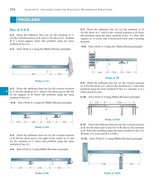
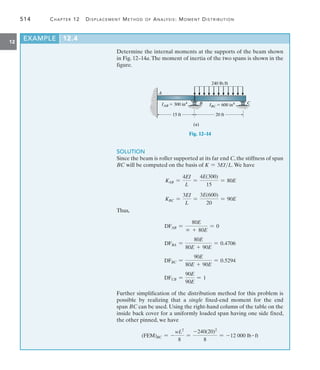
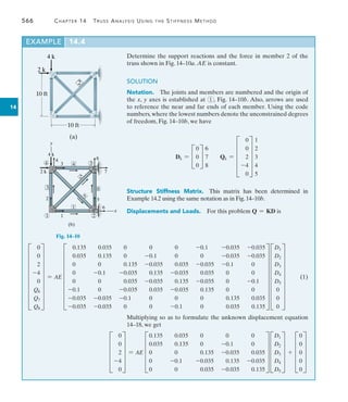
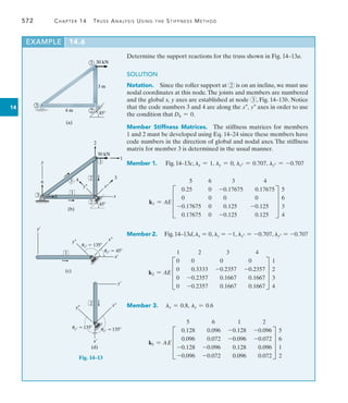
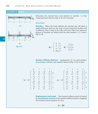
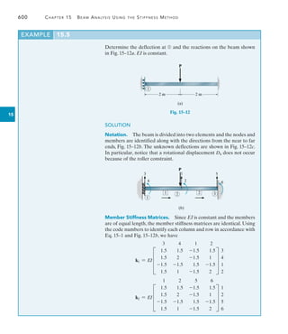
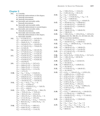
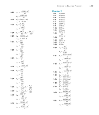
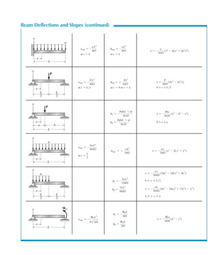
![598 Chapter 15 Beam Analysis Using the Stiffness Method
15
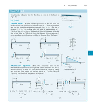
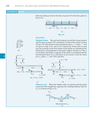
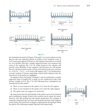
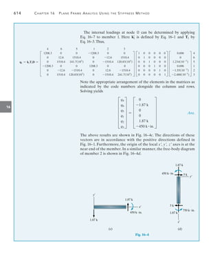
Determine the moment developed at support A of the beam shown in
Fig. 15–11a. Assume the roller supports can pull down or push up on
the beam.Take E = 29(103
) ksi, I = 510 in4
.
SOLUTION
Notation. Here the beam has two unconstrained degrees of freedom,
identified by the code numbers 1 and 2.
The matrix analysis requires that the external loading be applied at
the nodes, and therefore the distributed and concentrated loads are
replaced by their equivalent fixed-end moments,which are determined
from the table on the inside back cover. (See Example 11.2.) Note that
no external loads are placed at ➀ and no external vertical forces are
placed at ➁ since the reactions at code numbers 3, 4 and 5 are to be
unknowns in the load matrix. Using superposition, the results of the
matrix analysis for the loading in Fig. 15–11b will later be modified by
the loads shown in Fig. 15–11c. From Fig. 15–11b, the known
displacement and load matrices are
Dk = C
0
0
0
S
4
5
6
Qk = c
144
1008
d
1
2
Member Stiffness Matrices. Each of the two member stiffness
matrices is determined from Eq. 15–1.
Member 1:
12EI
L3
=
12(29)(103
)(510)
[24(12)]3
= 7.430
6EI
L2
=
6(29)(103
)(510)
[24(12)]2
= 1069.9
4EI
L
=
4(29)(103
)(510)
24(12)
= 205 417
2EI
L
=
2(29)(103
)(510)
24(12)
= 102 708
k1 =
4 3 5 2
D
7.430 1069.9 -7.430 1069.9
1069.9 205 417 -1069.9 102 708
-7.430 -1069.9 7.430 -1069.9
1069.9 102 708 -1069.9 205 417
T
4
3
5
2
Member 2:
12EI
L3
=
12(29)(103
)(510)
[8(12)]3
= 200.602
6EI
L2
=
6(29)(103
)(510)
[8(12)]2
= 9628.91
12 k
2 k/ft
A B
C
24 ft
4 ft 4 ft
(a)
1 1
3
4
96 kft 12 kft 1008 kin. 12 kft 144 kin.
2
5
2
6
1
2 2 3
beam to be analyzed by stiffness method
(b)
Fig. 15–11
12 k
2 k/ft
24 k
12 kft 144 kin.
96 kft 1152 kin.
beam subjected to actual load and
fixed-supported reactions
(c)
A B
C
24 k
6 k 6 k
EXAMPLE 15.4](https://image.slidesharecdn.com/structuralanalysis-hibbelerpdfdrive-220911133905-65f3c8d4/85/STRUCTURAL-ANALYSIS-NINTH-EDITION-R-C-HIBBELER-619-320.jpg)
![640
Appendix
A
Matrix Algebra for
Structural Analysis
A.1
Basic Definitions and Types
of Matrices
With the accessibility of desk top computers,application of matrix algebra
for the analysis of structures has become widespread. Matrix algebra
provides an appropriate tool for this analysis, since it is relatively easy to
formulate the solution in a concise form and then perform the actual
matrix manipulations using a computer.For this reason it is important that
the structural engineer be familiar with the fundamental operations of this
type of mathematics.
Matrix. A matrix is a rectangular arrangement of numbers having m
rows and n columns. The numbers, which are called elements, are
assembled within brackets. For example, the A matrix is written as:
A = D
a11 a12 g a1n
a21 a22 g a2n
f
am1 am2 g amn
T
Such a matrix is said to have an order of m * n (m by n). Notice that the
first subscript for an element denotes its row position and the second
subscript denotes its column position. In general, then, aij is the element
located in the ith row and jth column.
Row Matrix. If the matrix consists only of elements in a single row,
it is called a row matrix. For example, a 1 * n row matrix is written as
A = [a1 a2 g an]
Here only a single subscript is used to denote an element, since the row
subscript is always understood to be equal to 1, that is, a1 = a11, a2 = a12,
and so on.](https://image.slidesharecdn.com/structuralanalysis-hibbelerpdfdrive-220911133905-65f3c8d4/85/STRUCTURAL-ANALYSIS-NINTH-EDITION-R-C-HIBBELER-661-320.jpg)
![644 Appendix A Matrix Algebra for Structural Analysis
A
As a second example, consider
A = C
5 3
4 1
-2 8
S B = c
2 7
-3 4
d
Here again the product C = AB can be found since A has two columns
and B has two rows.The resulting matrix C will have three rows and two
columns.The elements are obtained as follows:
c11 = 5(2) + 3(-3) = 1 (first row of A times first column of B)
c12 = 5(7) + 3(4) = 47 (first row of A times second column of B)
c21 = 4(2) + 1(-3) = 5 (second row of A times first column of B)
c22 = 4(7) + 1(4) = 32 (second row of A times second column of B)
c31 = -2(2) + 8(-3) = -28 (third row of A times first column of B)
c32 = -2(7) + 8(4) = 18 (third row of A times second column of B)
The scheme for multiplication follows application of Eq.A–2.Thus,
C = C
1 47
5 32
-28 18
S
Notice also that BA does not exist, since written in this manner the
matrices are nonconformable.
The following rules apply to matrix multiplication.
1. In general the product of two matrices is not commutative:
AB BA(A–3)
2. The distributive law is valid:
A(B + C) = AB + AC(A–4)
3. The associative law is valid:
A(BC) = (AB)C(A–5)
Transposed Matrix. A matrix may be transposed by interchanging
its rows and columns. For example, if
A = C
a11 a12 a13
a21 a22 a23
a31 a32 a33
S B = [b1 b2 b3]](https://image.slidesharecdn.com/structuralanalysis-hibbelerpdfdrive-220911133905-65f3c8d4/85/STRUCTURAL-ANALYSIS-NINTH-EDITION-R-C-HIBBELER-665-320.jpg)
![A.2 Matrix Operations 645
A
Then
AT
= C
a11 a21 a31
a12 a22 a32
a13 a23 a33
S BT
= C
b1
b2
b3
S
Notice that AB is nonconformable and so the product does not exist.
(A has three columns and B has one row.) Alternatively, multiplication
ABT
is possible since here the matrices are conformable (A has three
columns and BT
has three rows).The following properties for transposed
matrices hold:
(A + B)T
= AT
+ BT
(A–6)
(kA)T
= kAT
(A–7)
(AB)T
= BT
AT
(A–8)
This last identity will be illustrated by example. If
A = c
6 2
1 -3
d B = c
4 3
2 5
d
Then, by Eq.A–8,
a c
6 2
1 -3
d c
4 3
2 5
d b
T
= c
4 2
3 5
d c
6 1
2 -3
d
a c
28 28
-2 -12
d b
T
= c
28 -2
28 -12
d
c
28 -2
28 -12
d = c
28 -2
28 -12
d
Matrix Partitioning. A matrix can be subdivided into submatrices
by partitioning. For example,
A = C
a11 a12 a13 a14
a21 a22 a23 a24
a31 a32 a33 a34
S = c
A11 A12
A21 A22
d
Here the submatrices are
A11 = [a11] A12 = [a12 a13 a14]
A21 = c
a21
a31
d A22 = c
a22 a23 a24
a32 a33 a34
d](https://image.slidesharecdn.com/structuralanalysis-hibbelerpdfdrive-220911133905-65f3c8d4/85/STRUCTURAL-ANALYSIS-NINTH-EDITION-R-C-HIBBELER-666-320.jpg)
![646 Appendix A Matrix Algebra for Structural Analysis
A
The rules of matrix algebra apply to partitioned matrices provided the
partitioning is conformable. For example, corresponding submatrices of
A and B can be added or subtracted provided they have an equal number
of rows and columns. Likewise, matrix multiplication is possible provided
the respective number of columns and rows of both A and B and their
submatrices are equal. For instance, if
A = C
4 1 -1
-2 0 -5
6 3 8
S B = C
2 -1
0 8
7 4
S
then the product AB exists, since the number of columns of A equals the
number of rows of B (three). Likewise, the partitioned matrices are
conformable for multiplication since A is partitioned into two columns
and B is partitioned into two rows, that is,
AB = c
A11 A12
A21 A22
d c
B11
B21
d = c
A11B11 + A12B21
A21B11 + A22B21
d
Multiplication of the submatrices yields
A11B11 = c
4 1
-2 0
d c
2 -1
0 8
d = c
8 4
-4 2
d
A12B21 = c
-1
-5
d [7 4] = c
-7 -4
-35 -20
d
A21B11 = [6 3]c
2 -1
0 8
d = [12 18]
A22B21 = [8][7 4] = [56 32]
AB = D
c
8
-4
4
2
d + c
-7
-35
-4
-20
d
[12 18] + [56 32]
T = C
1 0
-39 -18
68 50
S
A.3 Determinants
In the next section we will discuss how to invert a matrix. Since this
operation requires an evaluation of the determinant of the matrix, we will
now discuss some of the basic properties of determinants.
A determinant is a square array of numbers enclosed within vertical
bars. For example, an nth-order determinant, having n rows and n
columns, is
A = 4
a11 a12 g a1n
a21 a22 g a2n
f
an1 an2 g ann
4 (A–9)](https://image.slidesharecdn.com/structuralanalysis-hibbelerpdfdrive-220911133905-65f3c8d4/85/STRUCTURAL-ANALYSIS-NINTH-EDITION-R-C-HIBBELER-667-320.jpg)
![652 Appendix A Matrix Algebra for Structural Analysis
A
Problems
A–1. If A = c
4 2 -3
6 1 5
d and B = c
4 -1 0
2 0 8
d ,
determine A + B and A - 2B.
A–2. If A = c
3 5
-2 7
d , determine A + AT
.
A–3. If A = [6 1 3] and B = [1 6 3] show that
(A + B)T
= AT
+ BT
.
A–4. If A = C
1
0
5
S and B = [2 -1 3], determine AB.
A–5. If A = C
6 2 2
-5 1 1
0 3 1
S and B = C
-1 3 1
2 -5 1
0 7 5
S ,
determine AB.
A–6. Determine BA for the matrices of Prob.A–5.
A–7. If A = c
5 7
-2 1
d and B = c
6
7
d , determine AB.
A–8. If A = c
1 8 4
1 2 3
d and B = C
3
2
-6
S , determine AB.
A–9. If A = c
2 7 3
-2 1 0
d and B = C
6
9
-1
S , determine AB.
A–10. If A = C
6 4 2
2 1 1
0 -3 1
S and B = C
-1 3 -2
2 4 1
0 7 5
S ,
determine AB.](https://image.slidesharecdn.com/structuralanalysis-hibbelerpdfdrive-220911133905-65f3c8d4/85/STRUCTURAL-ANALYSIS-NINTH-EDITION-R-C-HIBBELER-673-320.jpg)
![Problems 653
A
A–11. If A = c
2 5
1 3
d , determine AAT
.
A–12. Show that the distributive law is valid, i.e.,
A(B + C) = AB + AC, if
A = c
2 1 6
4 5 3
d , B = C
3
1
-6
S , C = C
5
-1
2
S .
A–13. Show that the associative law is valid, i.e.,
A(BC) = (AB)C, if
A = c
2 1 6
4 5 3
d , B = C
3
1
-6
S , C = [5 -1 2].
A–14.
Evaluate the determinants `
2 5
7 1
` and
†
1 3 5
2 7 1
3 8 6
† .
A–15. If A = c
5 1
3 -2
d , determine A-1
.
A–16. If A = C
0 1 3
2 5 0
1 -1 2
S , determine A-1
.
A–17. Solve the equations -x1 + 4x2 + x3 = 1,
2x1 - x2 + x3 = 2, and 4x1 - 5x2 + 3x3 = 4 using the
matrix equation X = A-1
C.
A–18.
Solve the equations in Prob. A–17 using the Gauss
elimination method.
A–19. Solve the equations x1 - x2 + x3 = -1,
-x1 + x2 + x3 = -1, and x1 + 2x2 - 2x3 = 5 using the
matrix equation X = A-1
B.
A–20. Solve the equations in Prob. A–19 using the Gauss
elimination method.](https://image.slidesharecdn.com/structuralanalysis-hibbelerpdfdrive-220911133905-65f3c8d4/85/STRUCTURAL-ANALYSIS-NINTH-EDITION-R-C-HIBBELER-674-320.jpg)


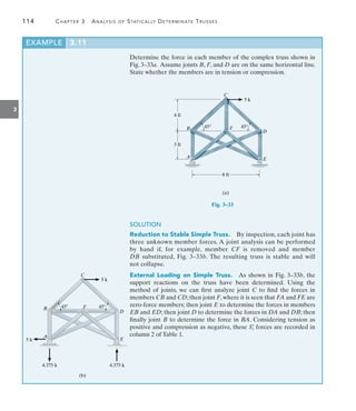
The ninth edition of 'Structural Analysis' by R.C. Hibbeler serves as a comprehensive guide for students to understand the theory and application of structural analysis to trusses, beams, and frames, with a focus on both classical and modern matrix methods. This edition includes significant updates such as new examples of structural failures, enhanced diagrams, and approximately 70% new problems to ensure a thorough grasp of concepts and improve problem-solving skills. Resources for both instructors and students are provided, including online tutorials, video solutions, and downloadable software for practical application of the material.