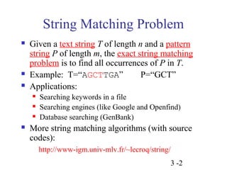
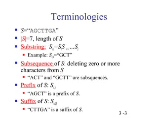
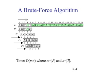
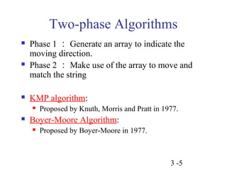
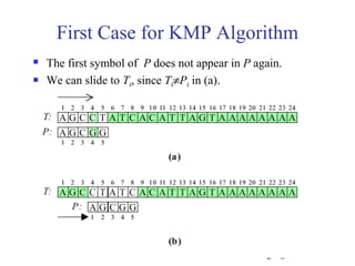
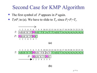
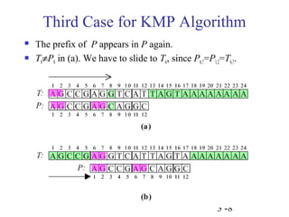
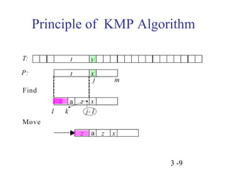
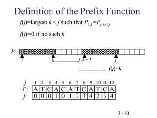
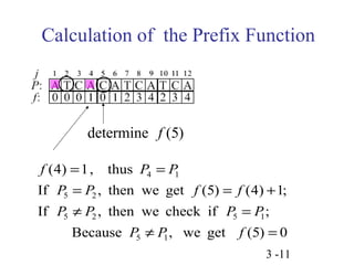
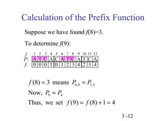
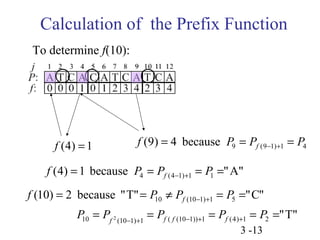
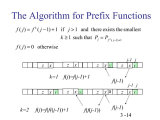
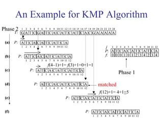
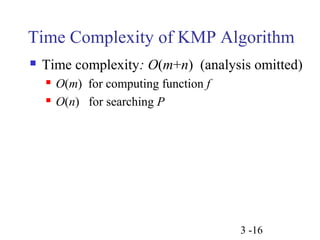
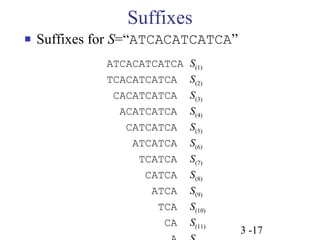
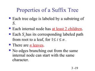
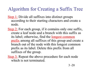
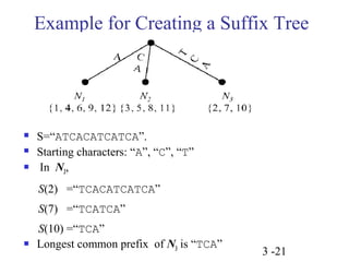
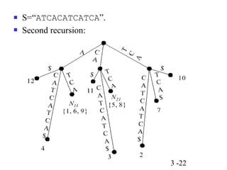
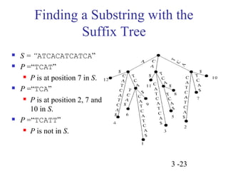
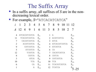
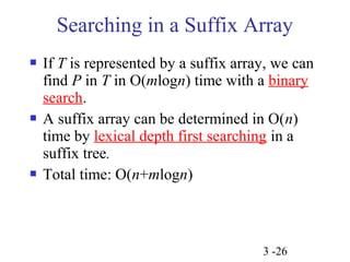
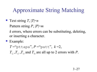
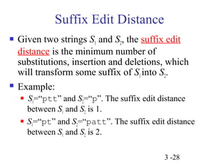
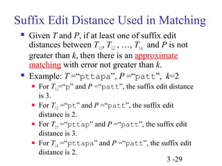
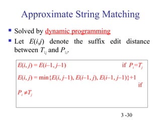
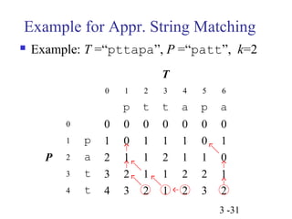
3 -1 
Chapter 3 
String Matching
String Matching Problem 
 Given a text string T of length n and a pattern 
string P of length m, the exact string matching 
problem is to find all occurrences of P in T. 
 Example: T=“AGCTTGA” P=“GCT” 
 Applications: 
 Searching keywords in a file 
 Searching engines (like Google and Openfind) 
 Database searching (GenBank) 
 More string matching algorithms (with source 
codes): 
http://www-igm.univ-mlv.fr/~lecroq/string/ 
3 -2
3 -3 
Terminologies 
 S=“AGCTTGA” 
 |S|=7, length of S 
 Substring: Si,j=SiS i+1…Sj 
 Example: S2,4=“GCT” 
 Subsequence of S: deleting zero or more 
characters from S 
 “ACT” and “GCTT” are subsquences. 
 Prefix of S: S1,k 
 “AGCT” is a prefix of S. 
 Suffix of S: Sh,|S| 
 “CTTGA” is a suffix of S.
A Brute-Force Algorithm 
3 -4 
Time: O(mn) where m=|P| and n=|T|.
Two-phase Algorithms 
 Phase 1:Generate an array to indicate the 
moving direction. 
 Phase 2:Make use of the array to move and 
match the string 
3 -5 
 KMP algorithm: 
 Proposed by Knuth, Morris and Pratt in 1977. 
 Boyer-Moore Algorithm: 
 Proposed by Boyer-Moore in 1977.
First Case for KMP Algorithm 
 The first symbol of P does not appear in P again. 
 We can slide to T4, since T4¹P4 in (a). 
3 -6
Second Case for KMP Algorithm 
 The first symbol of P appears in P again. 
 T7¹P7 in (a). We have to slide to T6, since P6=P1=T6. 
3 -7
Third Case for KMP Algorithm 
 The prefix of P appears in P again. 
 T8¹P8 in (a). We have to slide to T6, since P6,7=P1,2=T6,7. 
3 -8
Principle of KMP Algorithm 
3 -9 
a 
a
Definition of the Prefix Function 
f(j)=k 
3 -10 
f(j)=largest k < j such that P1,k=Pj–k+1,j 
f(j)=0 if no such k
Calculation of the Prefix Function 
f (4) = 1 , thus 
P = 
P 
P P f f 
= = + 
If , then we get (5) (4) 1; 
P ¹ P P = 
P 
If , then we check if ; 
3 -11 
determine f (5) 
5 2 5 1 
P P f 
Because , we get (5) 0 
5 1 
5 2 
4 1 
¹ =
Calculation of the Prefix Function 
Suppose we have found f(8)=3. 
To determine f(9): 
3 -12 
f (8) = 3 means 
P = 
P 
Now, 
P = 
P 
9 4 
6,8 1,3 
f f 
= + = 
Thus, we set (9) (8) 1 4
Calculation of the Prefix Function 
To determine f(10): 
f (4) = 1 9 (9 1) 1 4 f (9) 4 because P P P f = = = - + 
(4) 1 because "A" 4 (4 1) 1 1 = = = = - + f P P P f 
f P P P 
= = ¹ = = 
- + 
f 
P P P P P 
2 = = = = = 
f f f f 
- + - + + 
3 -13 
"T" 
(10) 2 because "T" "C" 
10 (10 1) 1 5 
10 (10 1) 1 ( (10 1)) 1 (4) 1 2
The Algorithm for Prefix Functions 
f j f j j 
= - + > 
( ) ( 1) 1 if 1 and there exists the smallest 
j-1 j 
3 -14 
a 
k=1 f(j)=f(j-1)+1 
k=2 f(j)=f(f((j-1))+1 
f(j-1) 
j-1 j 
f(f(j-1)) f(j-1) 
( ) 0 otherwise 
1 such that 
( 1) 1 
= 
³ = 
- + 
f j 
k P P 
j f j 
k 
k
An Example for KMP Algorithm 
Phase 1 
3 -15 
Phase 2 
f(4–1)+1= f(3)+1=0+1=1 
matched 
f(12)+1= 4+1=5
Time Complexity of KMP Algorithm 
 Time complexity: O(m+n) (analysis omitted) 
3 -16 
 O(m) for computing function f 
 O(n) for searching P
3 -17 
Suffixes 
 Suffixes for S=“ATCACATCATCA” 
ATCACATCATCA S(1) 
TCACATCATCA S(2) 
CACATCATCA S(3) 
ACATCATCA S(4) 
CATCATCA S(5) 
ATCATCA S(6) 
TCATCA S(7) 
CATCA S(8) 
ATCA S(9) 
TCA S(10) 
CA S(11) 
A S(12)
 A suffix Tree for S=“ATCACATCATCA” 
3 -18 
Suffix Trees
Properties of a Suffix Tree 
 Each tree edge is labeled by a substring of 
S. 
 Each internal node has at least 2 children. 
 Each S(i) has its corresponding labeled path 
from root to a leaf, for 1£ i £ n . 
 There are n leaves. 
 No edges branching out from the same 
internal node can start with the same 
character. 
3 -19
Algorithm for Creating a Suffix Tree 
Step 1: Divide all suffixes into distinct groups 
according to their starting characters and create a 
node. 
Step 2: For each group, if it contains only one suffix, 
create a leaf node and a branch with this suffix as 
its label; otherwise, find the longest common 
prefix among all suffixes of this group and create a 
branch out of the node with this longest common 
prefix as its label. Delete this prefix from all 
suffixes of the group. 
Step 3: Repeat the above procedure for each node 
which is not terminated. 
3 -20
Example for Creating a Suffix Tree 
3 -21 
 S=“ATCACATCATCA”. 
 Starting characters: “A”, “C”, “T” 
 In N3, 
S(2) =“TCACATCATCA” 
S(7) =“TCATCA” 
S(10) =“TCA” 
 Longest common prefix of N3 is “TCA”
3 -22 
 S=“ATCACATCATCA”. 
 Second recursion:
Finding a Substring with the 
3 -23 
Suffix Tree 
 S = “ATCACATCATCA” 
 P =“TCAT” 
 P is at position 7 in S. 
 P =“TCA” 
 P is at position 2, 7 and 
10 in S. 
 P =“TCATT” 
 P is not in S.
 A suffix tree for a text string T of length n 
can be constructed in O(n) time (with a 
complicated algorithm). 
 To search a pattern P of length m on a 
suffix tree needs O(m) comparisons. 
 Exact string matching: O(n+m) time 
3 -24 
Time Complexity
i 1 2 3 4 5 6 7 8 9 10 11 12 
A 12 4 9 1 6 11 3 8 5 10 2 7 
3 -25 
The Suffix Array 
 In a suffix array, all suffixes of S are in the non-decreasing 
lexical order. 
 For example, S=“ATCACATCATCA” 
4 ATCACATCATCA S(1) 
11 TCACATCATCA S(2) 
7 CACATCATCA S(3) 
2 ACATCATCA S(4) 
9 CATCATCA S(5) 
5 ATCATCA S(6) 
12 TCATCA S(7) 
8 CATCA S(8) 
3 ATCA S(9) 
10 TCA S(10) 
6 CA S(11) 
1 A S(12) 
1 A S(12) 
2 ACATCATCA S(4) 
3 ATCA S(9) 
4 ATCACATCATCA S(1) 
5 ATCATCA S(6) 
6 CA S(11) 
7 CACATCATCA S(3) 
8 CATCA S(8) 
9 CATCATCA S(5) 
10 TCA S(10) 
11 TCACATCATCA S(2) 
12 TCATCA S(7)
Searching in a Suffix Array 
 If T is represented by a suffix array, we can 
find P in T in O(mlogn) time with a binary 
search. 
 A suffix array can be determined in O(n) 
time by lexical depth first searching in a 
suffix tree. 
 Total time: O(n+mlogn) 
3 -26
Approximate String Matching 
 Text string T, |T|=n 
Pattern string P, |P|=m 
k errors, where errors can be substituting, deleting, 
or inserting a character. 
 Example: 
T =“pttapa”, P =“patt”, k =2, 
T1,2 ,T1,3 ,T1,4 and T5,6 are all up to 2 errors with P. 
3 -27
3 -28 
Suffix Edit Distance 
 Given two strings S1 and S2, the suffix edit 
distance is the minimum number of 
substitutions, insertion and deletions, which 
will transform some suffix of S1 into S2. 
 Example: 
 S1=“ptt” and S2=“p”. The suffix edit distance 
between S1 and S2 is 1. 
 S1=“pt” and S2=“patt”. The suffix edit distance 
between S1 and S2 is 2.
Suffix Edit Distance Used in Matching 
 Given T and P, if at least one of suffix edit 
distances between T1,1, T1,2 , …, T1,n and P is not 
greater than k, then there is an approximate 
matching with error not greater than k. 
 Example: T =“pttapa”, P =“patt”, k=2 
 For T1,1=“p” and P =“patt”, the suffix edit distance 
is 3. 
 For T1,2 =“pt” and P =“patt”, the suffix edit 
distance is 2. 
 For T1,5 =“pttap” and P =“patt”, the suffix edit 
distance is 3. 
 For T1,6 =“pttapa” and P =“patt”, the suffix edit 
distance is 2. 
3 -29
Approximate String Matching 
 Solved by dynamic programming 
 Let E(i,j) denote the suffix edit distance 
between T1,j and P1,i. 
E(i, j) = E(i–1, j–1) if Pi=Tj 
E(i, j) = min{E(i, j–1), E(i–1, j), E(i–1, j–1)}+1 
3 -30 
if 
Pi ¹Tj
Example for Appr. String Matching 
 Example: T =“pttapa”, P =“patt”, k=2 
3 -31 
T 
0 1 2 3 4 5 6 
p t t a p a 
P 
0 0 0 0 0 0 0 0 
1 p 1 0 1 1 1 0 1 
2 a 2 1 1 2 1 1 0 
3 t 3 2 1 1 2 2 1 
4 t 4 3 2 1 2 3 2

String kmp

  • 1.
    3 -1 Chapter3 String Matching
  • 2.
    String Matching Problem  Given a text string T of length n and a pattern string P of length m, the exact string matching problem is to find all occurrences of P in T.  Example: T=“AGCTTGA” P=“GCT”  Applications:  Searching keywords in a file  Searching engines (like Google and Openfind)  Database searching (GenBank)  More string matching algorithms (with source codes): http://www-igm.univ-mlv.fr/~lecroq/string/ 3 -2
  • 3.
    3 -3 Terminologies  S=“AGCTTGA”  |S|=7, length of S  Substring: Si,j=SiS i+1…Sj  Example: S2,4=“GCT”  Subsequence of S: deleting zero or more characters from S  “ACT” and “GCTT” are subsquences.  Prefix of S: S1,k  “AGCT” is a prefix of S.  Suffix of S: Sh,|S|  “CTTGA” is a suffix of S.
  • 4.
    A Brute-Force Algorithm 3 -4 Time: O(mn) where m=|P| and n=|T|.
  • 5.
    Two-phase Algorithms Phase 1:Generate an array to indicate the moving direction.  Phase 2:Make use of the array to move and match the string 3 -5  KMP algorithm:  Proposed by Knuth, Morris and Pratt in 1977.  Boyer-Moore Algorithm:  Proposed by Boyer-Moore in 1977.
  • 6.
    First Case forKMP Algorithm  The first symbol of P does not appear in P again.  We can slide to T4, since T4¹P4 in (a). 3 -6
  • 7.
    Second Case forKMP Algorithm  The first symbol of P appears in P again.  T7¹P7 in (a). We have to slide to T6, since P6=P1=T6. 3 -7
  • 8.
    Third Case forKMP Algorithm  The prefix of P appears in P again.  T8¹P8 in (a). We have to slide to T6, since P6,7=P1,2=T6,7. 3 -8
  • 9.
    Principle of KMPAlgorithm 3 -9 a a
  • 10.
    Definition of thePrefix Function f(j)=k 3 -10 f(j)=largest k < j such that P1,k=Pj–k+1,j f(j)=0 if no such k
  • 11.
    Calculation of thePrefix Function f (4) = 1 , thus P = P P P f f = = + If , then we get (5) (4) 1; P ¹ P P = P If , then we check if ; 3 -11 determine f (5) 5 2 5 1 P P f Because , we get (5) 0 5 1 5 2 4 1 ¹ =
  • 12.
    Calculation of thePrefix Function Suppose we have found f(8)=3. To determine f(9): 3 -12 f (8) = 3 means P = P Now, P = P 9 4 6,8 1,3 f f = + = Thus, we set (9) (8) 1 4
  • 13.
    Calculation of thePrefix Function To determine f(10): f (4) = 1 9 (9 1) 1 4 f (9) 4 because P P P f = = = - + (4) 1 because "A" 4 (4 1) 1 1 = = = = - + f P P P f f P P P = = ¹ = = - + f P P P P P 2 = = = = = f f f f - + - + + 3 -13 "T" (10) 2 because "T" "C" 10 (10 1) 1 5 10 (10 1) 1 ( (10 1)) 1 (4) 1 2
  • 14.
    The Algorithm forPrefix Functions f j f j j = - + > ( ) ( 1) 1 if 1 and there exists the smallest j-1 j 3 -14 a k=1 f(j)=f(j-1)+1 k=2 f(j)=f(f((j-1))+1 f(j-1) j-1 j f(f(j-1)) f(j-1) ( ) 0 otherwise 1 such that ( 1) 1 = ³ = - + f j k P P j f j k k
  • 15.
    An Example forKMP Algorithm Phase 1 3 -15 Phase 2 f(4–1)+1= f(3)+1=0+1=1 matched f(12)+1= 4+1=5
  • 16.
    Time Complexity ofKMP Algorithm  Time complexity: O(m+n) (analysis omitted) 3 -16  O(m) for computing function f  O(n) for searching P
  • 17.
    3 -17 Suffixes  Suffixes for S=“ATCACATCATCA” ATCACATCATCA S(1) TCACATCATCA S(2) CACATCATCA S(3) ACATCATCA S(4) CATCATCA S(5) ATCATCA S(6) TCATCA S(7) CATCA S(8) ATCA S(9) TCA S(10) CA S(11) A S(12)
  • 18.
     A suffixTree for S=“ATCACATCATCA” 3 -18 Suffix Trees
  • 19.
    Properties of aSuffix Tree  Each tree edge is labeled by a substring of S.  Each internal node has at least 2 children.  Each S(i) has its corresponding labeled path from root to a leaf, for 1£ i £ n .  There are n leaves.  No edges branching out from the same internal node can start with the same character. 3 -19
  • 20.
    Algorithm for Creatinga Suffix Tree Step 1: Divide all suffixes into distinct groups according to their starting characters and create a node. Step 2: For each group, if it contains only one suffix, create a leaf node and a branch with this suffix as its label; otherwise, find the longest common prefix among all suffixes of this group and create a branch out of the node with this longest common prefix as its label. Delete this prefix from all suffixes of the group. Step 3: Repeat the above procedure for each node which is not terminated. 3 -20
  • 21.
    Example for Creatinga Suffix Tree 3 -21  S=“ATCACATCATCA”.  Starting characters: “A”, “C”, “T”  In N3, S(2) =“TCACATCATCA” S(7) =“TCATCA” S(10) =“TCA”  Longest common prefix of N3 is “TCA”
  • 22.
    3 -22 S=“ATCACATCATCA”.  Second recursion:
  • 23.
    Finding a Substringwith the 3 -23 Suffix Tree  S = “ATCACATCATCA”  P =“TCAT”  P is at position 7 in S.  P =“TCA”  P is at position 2, 7 and 10 in S.  P =“TCATT”  P is not in S.
  • 24.
     A suffixtree for a text string T of length n can be constructed in O(n) time (with a complicated algorithm).  To search a pattern P of length m on a suffix tree needs O(m) comparisons.  Exact string matching: O(n+m) time 3 -24 Time Complexity
  • 25.
    i 1 23 4 5 6 7 8 9 10 11 12 A 12 4 9 1 6 11 3 8 5 10 2 7 3 -25 The Suffix Array  In a suffix array, all suffixes of S are in the non-decreasing lexical order.  For example, S=“ATCACATCATCA” 4 ATCACATCATCA S(1) 11 TCACATCATCA S(2) 7 CACATCATCA S(3) 2 ACATCATCA S(4) 9 CATCATCA S(5) 5 ATCATCA S(6) 12 TCATCA S(7) 8 CATCA S(8) 3 ATCA S(9) 10 TCA S(10) 6 CA S(11) 1 A S(12) 1 A S(12) 2 ACATCATCA S(4) 3 ATCA S(9) 4 ATCACATCATCA S(1) 5 ATCATCA S(6) 6 CA S(11) 7 CACATCATCA S(3) 8 CATCA S(8) 9 CATCATCA S(5) 10 TCA S(10) 11 TCACATCATCA S(2) 12 TCATCA S(7)
  • 26.
    Searching in aSuffix Array  If T is represented by a suffix array, we can find P in T in O(mlogn) time with a binary search.  A suffix array can be determined in O(n) time by lexical depth first searching in a suffix tree.  Total time: O(n+mlogn) 3 -26
  • 27.
    Approximate String Matching  Text string T, |T|=n Pattern string P, |P|=m k errors, where errors can be substituting, deleting, or inserting a character.  Example: T =“pttapa”, P =“patt”, k =2, T1,2 ,T1,3 ,T1,4 and T5,6 are all up to 2 errors with P. 3 -27
  • 28.
    3 -28 SuffixEdit Distance  Given two strings S1 and S2, the suffix edit distance is the minimum number of substitutions, insertion and deletions, which will transform some suffix of S1 into S2.  Example:  S1=“ptt” and S2=“p”. The suffix edit distance between S1 and S2 is 1.  S1=“pt” and S2=“patt”. The suffix edit distance between S1 and S2 is 2.
  • 29.
    Suffix Edit DistanceUsed in Matching  Given T and P, if at least one of suffix edit distances between T1,1, T1,2 , …, T1,n and P is not greater than k, then there is an approximate matching with error not greater than k.  Example: T =“pttapa”, P =“patt”, k=2  For T1,1=“p” and P =“patt”, the suffix edit distance is 3.  For T1,2 =“pt” and P =“patt”, the suffix edit distance is 2.  For T1,5 =“pttap” and P =“patt”, the suffix edit distance is 3.  For T1,6 =“pttapa” and P =“patt”, the suffix edit distance is 2. 3 -29
  • 30.
    Approximate String Matching  Solved by dynamic programming  Let E(i,j) denote the suffix edit distance between T1,j and P1,i. E(i, j) = E(i–1, j–1) if Pi=Tj E(i, j) = min{E(i, j–1), E(i–1, j), E(i–1, j–1)}+1 3 -30 if Pi ¹Tj
  • 31.
    Example for Appr.String Matching  Example: T =“pttapa”, P =“patt”, k=2 3 -31 T 0 1 2 3 4 5 6 p t t a p a P 0 0 0 0 0 0 0 0 1 p 1 0 1 1 1 0 1 2 a 2 1 1 2 1 1 0 3 t 3 2 1 1 2 2 1 4 t 4 3 2 1 2 3 2