Outline
Repeat Finding
Hash Tables
Exact Pattern Matching
Keyword Trees
Suffix Trees
Suffix Array
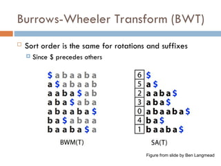
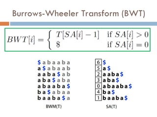
Burrows-Wheeler Transform (BWT)
FM Index
3.
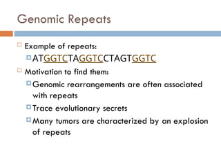
Genomic Repeats
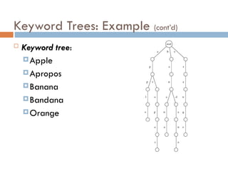
Exampleof repeats:
ATGGTCTAGGTCCTAGTGGTC
Motivation to find them:
Genomic rearrangements are often associated
with repeats
Trace evolutionary secrets
Many tumors are characterized by an explosion
of repeats
4.
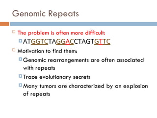
Genomic Repeats
Theproblem is often more difficult:
ATGGTCTAGGACCTAGTGTTC
Motivation to find them:
Genomic rearrangements are often associated
with repeats
Trace evolutionary secrets
Many tumors are characterized by an explosion
of repeats
5.
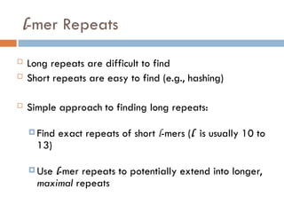
l-mer Repeats
Longrepeats are difficult to find
Short repeats are easy to find (e.g., hashing)
Simple approach to finding long repeats:
Find exact repeats of short l-mers (l is usually 10 to
13)
Use l-mer repeats to potentially extend into longer,
maximal repeats
6.
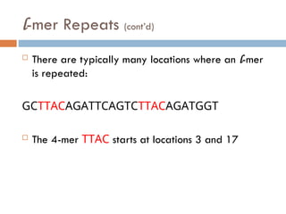
l-mer Repeats (cont’d)
There are typically many locations where an l-mer
is repeated:
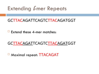
GCTTACAGATTCAGTCTTACAGATGGT
The 4-mer TTAC starts at locations 3 and 17
Maximal Repeats
Tofind maximal repeats in this way, we need ALL
start locations of all l-mers in the genome
Hashing lets us find repeats quickly in this manner
9.
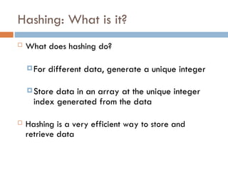
Hashing: What isit?
What does hashing do?
For different data, generate a unique integer
Store data in an array at the unique integer
index generated from the data
Hashing is a very efficient way to store and
retrieve data
10.
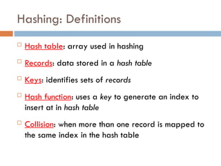
Hashing: Definitions
Hashtable: array used in hashing
Records: data stored in a hash table
Keys: identifies sets of records
Hash function: uses a key to generate an index to
insert at in hash table
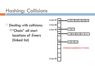
Collision: when more than one record is mapped to
the same index in the hash table
11.
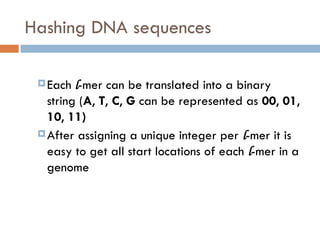
Hashing DNA sequences
Eachl-mer can be translated into a binary
string (A, T, C, G can be represented as 00, 01,
10, 11)
After assigning a unique integer per l-mer it is
easy to get all start locations of each l-mer in a
genome
12.
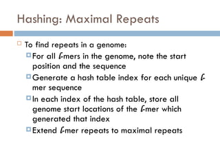
Hashing: Maximal Repeats
To find repeats in a genome:
For all l-mers in the genome, note the start
position and the sequence
Generate a hash table index for each unique l-
mer sequence
In each index of the hash table, store all
genome start locations of the l-mer which
generated that index
Extend l-mer repeats to maximal repeats
Hashing: Summary
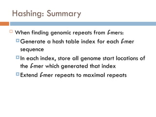
Whenfinding genomic repeats from l-mers:
Generate a hash table index for each l-mer
sequence
In each index, store all genome start locations of
the l-mer which generated that index
Extend l-mer repeats to maximal repeats
15.
Exact pattern matching
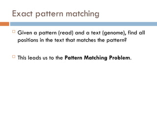
Given a pattern (read) and a text (genome), find all
positions in the text that matches the pattern?
This leads us to the Pattern Matching Problem.
16.
Pattern Matching Problem
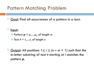
Goal: Find all occurrences of a pattern in a text.
Input:
Pattern p = p1…pm of length m
Text t = t1…tn of length n
Output: All positions 1< i < (n – m + 1) such that the
m-letter substring of text t starting at i matches the
pattern p.
17.
Exact Pattern Matching:Brute Force
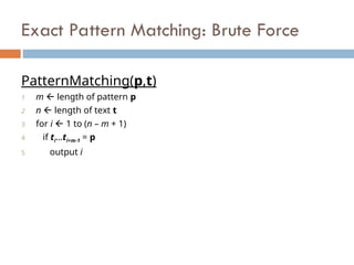
PatternMatching(p,t)
1 m length of pattern p
2 n length of text t
3 for i 1 to (n – m + 1)
4 if ti…ti+m-1 = p
5 output i
18.
Exact Pattern Matching:An Example
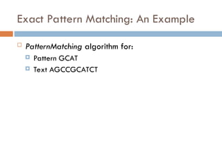
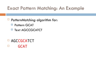
PatternMatching algorithm for:
Pattern GCAT
Text AGCCGCATCT
19.
Exact Pattern Matching:An Example
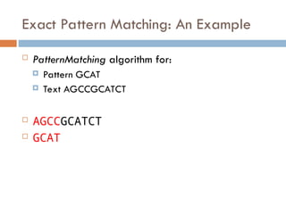
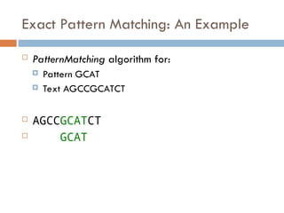
PatternMatching algorithm for:
Pattern GCAT
Text AGCCGCATCT
AGCCGCATCT
GCAT
20.
Exact Pattern Matching:An Example
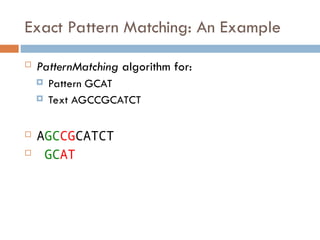
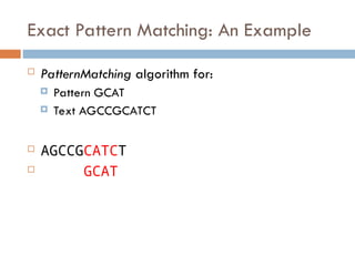
PatternMatching algorithm for:
Pattern GCAT
Text AGCCGCATCT
AGCCGCATCT
GCAT
21.
Exact Pattern Matching:An Example
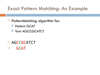
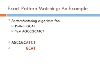
PatternMatching algorithm for:
Pattern GCAT
Text AGCCGCATCT
AGCCGCATCT
GCAT
22.
Exact Pattern Matching:An Example
PatternMatching algorithm for:
Pattern GCAT
Text AGCCGCATCT
AGCCGCATCT
GCAT
23.
Exact Pattern Matching:An Example
PatternMatching algorithm for:
Pattern GCAT
Text AGCCGCATCT
AGCCGCATCT
GCAT
24.
Exact Pattern Matching:An Example
PatternMatching algorithm for:
Pattern GCAT
Text AGCCGCATCT
AGCCGCATCT
GCAT
25.
Exact Pattern Matching:An Example
PatternMatching algorithm for:
Pattern GCAT
Text AGCCGCATCT
AGCCGCATCT
GCAT
26.
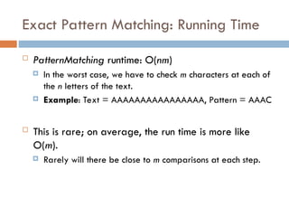
Exact Pattern Matching:Running Time
PatternMatching runtime: O(nm)
In the worst case, we have to check m characters at each of
the n letters of the text.
Example: Text = AAAAAAAAAAAAAAAA, Pattern = AAAC
This is rare; on average, the run time is more like
O(m).
Rarely will there be close to m comparisons at each step.
27.
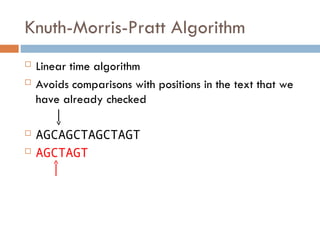
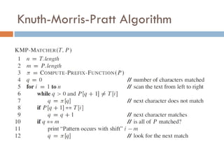
Knuth-Morris-Pratt Algorithm
Lineartime algorithm
Avoids comparisons with positions in the text that we
have already checked
AGCAGCTAGCTAGT
AGCTAGT
28.
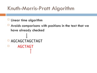
Knuth-Morris-Pratt Algorithm
Lineartime algorithm
Avoids comparisons with positions in the text that we
have already checked
AGCAGCTAGCTAGT
AGCTAGT
29.
Knuth-Morris-Pratt Algorithm
Pattern Matchedso far
AGCTAGT AGCTAG
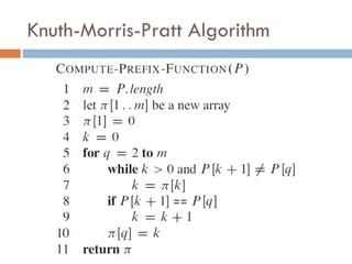
Compute length of the longest proper prefix of the
pattern P that is a proper suffix of P[1:q]
P[1:q] matched with the text at some point, but
p[q+1] failed.
Proper suffix
Proper prefix
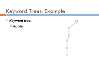
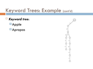
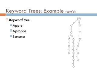
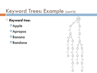
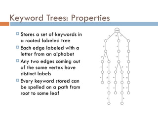
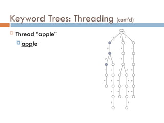
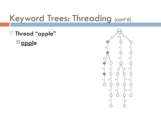
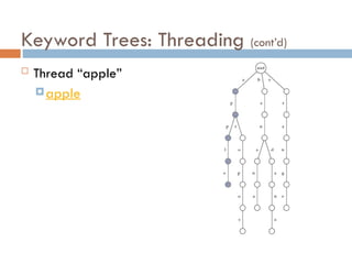
Keyword Trees: Properties
Stores a set of keywords in
a rooted labeled tree
Each edge labeled with a
letter from an alphabet
Any two edges coming out
of the same vertex have
distinct labels
Every keyword stored can
be spelled on a path from
root to some leaf
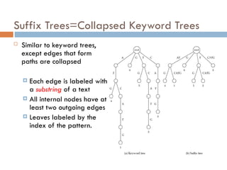
Suffix Trees=Collapsed KeywordTrees
Similar to keyword trees,
except edges that form
paths are collapsed
Each edge is labeled with
a substring of a text
All internal nodes have at
least two outgoing edges
Leaves labeled by the
index of the pattern.
52.
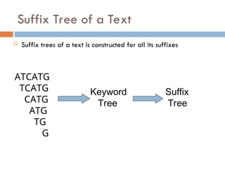
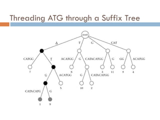
Suffix Tree ofa Text
Suffix trees of a text is constructed for all its suffixes
ATCATG
TCATG
CATG
ATG
TG
G
Keyword
Tree
Suffix
Tree
53.
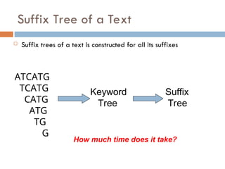
Suffix Tree ofa Text
Suffix trees of a text is constructed for all its suffixes
ATCATG
TCATG
CATG
ATG
TG
G
Keyword
Tree
Suffix
Tree
How much time does it take?
54.
Suffix Tree ofa Text
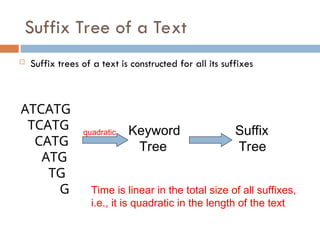
Suffix trees of a text is constructed for all its suffixes
ATCATG
TCATG
CATG
ATG
TG
G
quadratic Keyword
Tree
Suffix
Tree
Time is linear in the total size of all suffixes,
i.e., it is quadratic in the length of the text
55.
Suffix Trees: Advantages
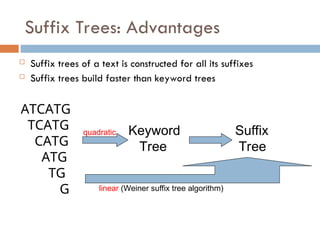
Suffix trees of a text is constructed for all its suffixes
Suffix trees build faster than keyword trees
ATCATG
TCATG
CATG
ATG
TG
G
quadratic Keyword
Tree
Suffix
Tree
linear (Weiner suffix tree algorithm)
56.
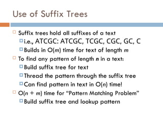
Use of SuffixTrees
Suffix trees hold all suffixes of a text
i.e., ATCGC: ATCGC, TCGC, CGC, GC, C
Builds in O(m) time for text of length m
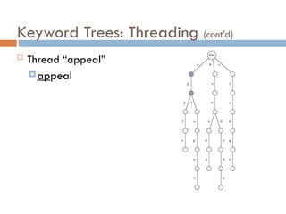
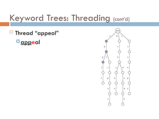
To find any pattern of length n in a text:
Build suffix tree for text
Thread the pattern through the suffix tree
Can find pattern in text in O(n) time!
O(n + m) time for “Pattern Matching Problem”
Build suffix tree and lookup pattern
57.
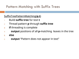
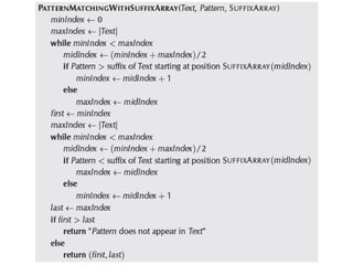
Pattern Matching withSuffix Trees
SuffixTreePatternMatching(p,t)
1 Build suffix tree for text t
2 Thread pattern p through suffix tree
3 if threading is complete
4 output positions of all p-matching leaves in the tree
5 else
6 output “Pattern does not appear in text”
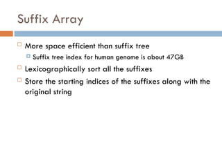
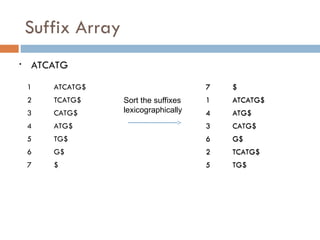
Suffix Array
Morespace efficient than suffix tree
Suffix tree index for human genome is about 47GB
Lexicographically sort all the suffixes
Store the starting indices of the suffixes along with the
original string
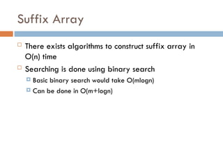
Suffix Array
Thereexists algorithms to construct suffix array in
O(n) time
Searching is done using binary search
Basic binary search would take O(mlogn)
Can be done in O(m+logn)
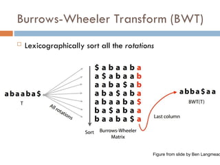
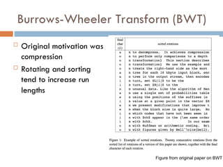
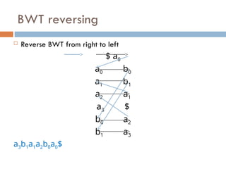
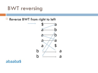
Burrows-Wheeler Transform (BWT)
Original motivation was
compression
Rotating and sorting
tend to increase run
lengths
Figure from original paper on BWT
67.
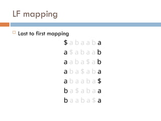
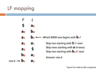
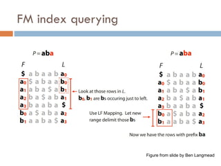
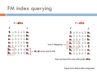
LF mapping
Lastto first mapping
$ a b a a b a
a $ a b a a b
a a b a $ a b
a b a $ a b a
a b a a b a $
b a $ a b a a
b a a b a $ a
68.
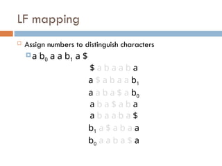
LF mapping
Assignnumbers to distinguish characters
a b0 a a b1 a $
$ a b a a b a
a $ a b a a b1
a a b a $ a b0
a b a $ a b a
a b a a b a $
b1 a $ a b a a
b0 a a b a $ a
69.
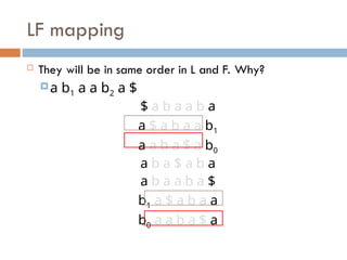
LF mapping
Theywill be in same order in L and F. Why?
a b1 a a b2 a $
$ a b a a b a
a $ a b a a b1
a a b a $ a b0
a b a $ a b a
a b a a b a $
b1 a $ a b a a
b0 a a b a $ a
70.
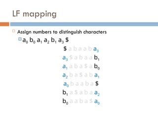
LF mapping
Assignnumbers to distinguish characters
a0 b0 a1 a2 b1 a3 $
$ a b a a b a3
a3 $ a b a a b1
a1 a b a $ a b0
a2 b a $ a b a1
a0 b a a b a $
b1 a $ a b a a2
b0 a a b a $ a0
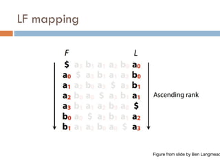
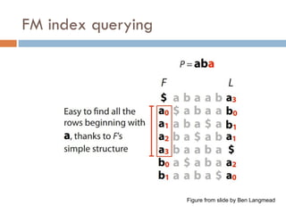
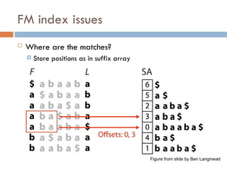
FM index issues
Where are the matches?
Store positions as in suffix array
Figure from slide by Ben Langmead
80.
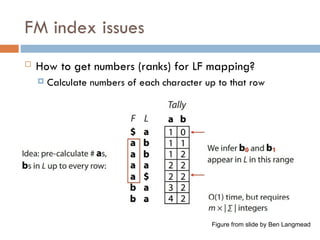
FM index issues
How to get numbers (ranks) for LF mapping?
Calculate numbers of each character up to that row
Figure from slide by Ben Langmead
81.
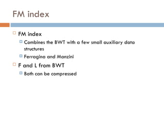
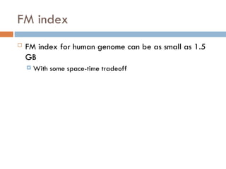
FM index
FMindex for human genome can be as small as 1.5
GB
With some space-time tradeoff
82.
References
Suffix Tree
Bioinformatics Algorithms (Part II) - Chapter 9
Part I of Algorithms on Strings, Trees and Sequences by Dan
Gusfield
BWT, FM index
http://www.cs.jhu.edu/~langmea/resources/bwt_fm.pdf
Editor's Notes
#29 Pi[q] is the length of the longest prefix of pattern P that is a proper suffix of P[1:q]. Here, P[1:q] matched with the text at some point, but p[q+1] failed.

![Knuth-Morris-Pratt Algorithm
Pattern Matched so far
AGCTAGT AGCTAG
Compute length of the longest proper prefix of the
pattern P that is a proper suffix of P[1:q]
P[1:q] matched with the text at some point, but
p[q+1] failed.
Proper suffix
Proper prefix](https://image.slidesharecdn.com/week11combinatorialpatternmatching1-251111171832-3442b001/85/Week_11_CombinatorialPatternMatching-of-bioinfo-29-320.jpg)
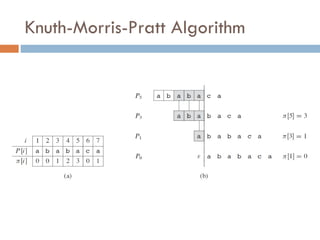
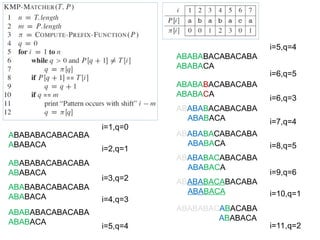
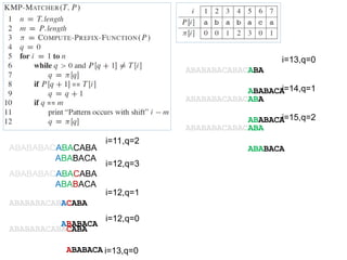
![ABABACA
ABABACA
k=0,П[1]=0,q=2
ABABACA
ABABACA
k=0,П[2]=0,q=3
ABABACA
ABABACA
ABABACA
ABABACA
ABABACA
ABABACA
ABABACA
ABABACA
k=1,П[5]=3,q=6
k=0,П[5]=3,q=6
k=1,П[3]=1,q=4
k=2,П[4]=2,q=5
k=3,П[5]=3,q=6
ABABACA
ABABACA
k=0,П[6]=0,q=7
ABABACA
ABABACA
k=1,П[7]=1,q=8
k=1,П[5]=3,q=6](https://image.slidesharecdn.com/week11combinatorialpatternmatching1-251111171832-3442b001/85/Week_11_CombinatorialPatternMatching-of-bioinfo-35-320.jpg)