The document outlines a proposed Ph.D. thesis focused on stream flow forecasting using artificial neural networks (ANN) and various data preprocessing techniques. It emphasizes the importance of accurately predicting stream flows for hydrologic applications and includes a detailed methodology for model development utilizing time series data from a gauging station along the Brahmaputra River. The study aims to evaluate different ANN architectures and preprocessing strategies to enhance forecasting performance.

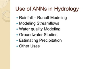
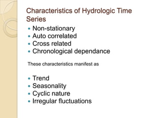
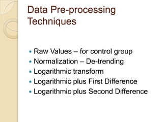
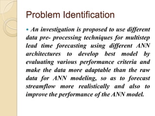
1. Stream flow Forecasting
by
ANN Modeling with
Preprocessing Techniques
for
Time Series Data
PROPOSAL FOR Ph.D. Thesis at N.I.T.K.
,Surathkal,
By Aniruddha Banhatti,
Part Time Ph.D. Student,
Registration Number: AM08P05

2. Importance of Stream Flow
Forecasting
 Hydrologic Structures
 Irrigation
 Flood Control
 Hydrologic Planning
 Flood Relief

3. Nature of Stream flow Data
 Time Series Data
 Show following characteristics:
 Trend
 Seasonality
 Cyclic Nature
 Irregular Fluctuations – Outliers and
Noise

4. Basics of Artificial Neural
Networks
 ANN is a massively parallel information
processing system.
 It resembles biological neural networks of
human brain.
 Processing occurs at large number of single
elements called Nodes or Neurons.
 Signals are passed between neurons using
Links
 Each link has a weight associated with it.
 Each link applies a nonlinear transformation
called an Activation Function to its net input

5. Schematic representation of
ANN

6. connectionsneurons
INPUT
LAYER
HIDDEN
LAYER
OUTPUT
LAYER
neurons
Each connection is
associated with a
particular weight
between 0 and 1
6

7. Structure of ANN
7
w
k1
x1
w
k2
x2
w
k
m
xm
...
...
Bias
bk
(.)vk
Input
Signal
Synaptic
Weights
Summing
Junction
Activation
Function
Output
yk
xwv j
m
j
kjk
0
)(vy kk

8. Algorithms for ANNs
Various algorithms can be used such
as :
 Back Propagation Algorithm
 Conjugate Gradient Algorithms
 Radial Basis Function
 Cascade Correlation Algorithm
 Recurrent ANNs
 Self Organizing feature Maps

9. Back Propagation Algorithm
is found to be best suited for
Time Series Data
and most of the
Hydrologic Modeling Problems.

10. Schematic of BP Algorithm

11. Use of ANNs in Hydrology
 Rainfall – Runoff Modeling
 Modeling Streamflows
 Water quality Modeling
 Groundwater Studies
 Estimating Precipitation
 Other Uses

12. Characteristics of Hydrologic Time
Series
 Non-stationary
 Auto correlated
 Cross related
 Chronological dependance
These characteristics manifest as
 Trend
 Seasonality
 Cyclic nature
 Irregular fluctuations

13. Data Pre-processing
Techniques
 Raw Values – for control group
 Normalization – De-trending
 Logarithmic transform
 Logarithmic plus First Difference
 Logarithmic plus Second Difference

14. Problem Identification
 An investigation is proposed to use different
data pre- processing techniques for multistep
lead time forecasting using different ANN
architectures to develop best model by
evaluating various performance criteria and
make the data more adaptable than the raw
data for ANN modeling, so as to forecast
streamflow more realistically and also to
improve the performance of the ANN model.

15. Study Area
 Gauging station at Pandu along
Brahmaputra River at Guwahati is
taken as the study area.
 Daily stream flow data for ten year
period
1st January 1990 to 31st December
1999
will be used for the present study.

16. Map of Study Area

17. Map of Study Area

18. Plan Of Research Work
 Plotting and Visual Observation of
Data
 Identification of Features Specific to
the Data
 Applying Pre-Processing Techniques
 Preparation of Data Sets

19. Data Sets
No. of lagged terms Dataset Lagged terms Data Matrix
Input Output
1 Raw values
Log
Log + first
difference
yt = xt
yt = log xt
yt = log xt + first diff.
y1
y2
y3
…..
yt
y2
y3
y4
…..
yt-1
2 Raw values
Log
Log + first
difference
yt = xt
yt = log xt
yt = log xt + first diff.
y1, y2
y2, y3
.….
yt-1, yt
y3
y4
.….
yt-2
3 Raw values
Log
Log + first
difference
yt = xt
yt = log xt
yt = log xt + first diff.
y1, y2, y3
y2, y3, y4
…..
…..
yt-2, yt-1,
yt
y4
y5
…..
…..
yt-3

20. Architectures of ANN
 According to Activating Function
 According to Number of Neurons
 According to Algorithm Used

21. Different Activating Functions

22. Architectures Used
According to Activation Function
 Sigmoid
 Tansig
 Logsig
According to number of input neurons
1 to 10
Input Neurons will be used

23. Number of Trials
 Nine Datasets
 Three Architectures
 Ten Input Methods
Thus there will be
9 X 3 X 10 = 270
Model Trials

24. Data Partitioning

25. Analysis
 Evaluation and Plotting of 270 Trials
 Evaluation Criteria
 RMSE
 MAPE
 R-Squared

26. Schedule
Month May
2011
Jun
2011
Jul
2011
Aug
2011
Sep
2011
Oct
2011
Nov
2011
Dec
2011
Making Datasets
Preliminary Trials
Progress Monitoring with
Guide
Completion of All Trials
Plotting of Results
Preparation of
Thesis