Call Girls Bommasandra Just Call 👗 7737669865 👗 Top Class Call Girl Service B...
Scholastic process and explaination lectr14.ppt
1. 1
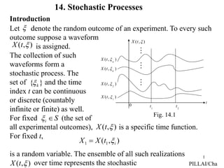
Let denote the random outcome of an experiment. To every such
outcome suppose a waveform
is assigned.
The collection of such
waveforms form a
stochastic process. The
set of and the time
index t can be continuous
or discrete (countably
infinite or finite) as well.
For fixed (the set of
all experimental outcomes), is a specific time function.
For fixed t,
is a random variable. The ensemble of all such realizations
over time represents the stochastic
)
,
(
t
X
}
{ k
S
i
)
,
( 1
1 i
t
X
X
)
,
(
t
X
PILLAI/Cha
14. Stochastic Processes
t
1
t 2
t
)
,
( n
t
X
)
,
( k
t
X
)
,
( 2
t
X
)
,
( 1
t
X
Fig. 14.1
)
,
(
t
X
0
)
,
(
t
X
Introduction
2. 2
process X(t). (see Fig 14.1). For example
where is a uniformly distributed random variable in
represents a stochastic process. Stochastic processes are everywhere:
Brownian motion, stock market fluctuations, various queuing systems
all represent stochastic phenomena.
If X(t) is a stochastic process, then for fixed t, X(t) represents
a random variable. Its distribution function is given by
Notice that depends on t, since for a different t, we obtain
a different random variable. Further
represents the first-order probability density function of the
process X(t).
),
cos(
)
( 0
t
a
t
X
}
)
(
{
)
,
( x
t
X
P
t
x
FX
)
,
( t
x
FX
(14-1)
(14-2)
PILLAI/Cha
(0,2 ),
dx
t
x
dF
t
x
f X
X
)
,
(
)
,
(
3. 3
For t = t1 and t = t2, X(t) represents two different random variables
X1 = X(t1) and X2 = X(t2) respectively. Their joint distribution is
given by
and
represents the second-order density function of the process X(t).
Similarly represents the nth order density
function of the process X(t). Complete specification of the stochastic
process X(t) requires the knowledge of
for all and for all n. (an almost impossible task
in reality).
}
)
(
,
)
(
{
)
,
,
,
( 2
2
1
1
2
1
2
1 x
t
X
x
t
X
P
t
t
x
x
FX
(14-3)
(14-4)
)
,
,
,
,
,
( 2
1
2
1 n
n t
t
t
x
x
x
fX
)
,
,
,
,
,
( 2
1
2
1 n
n t
t
t
x
x
x
fX
n
i
ti ,
,
2
,
1
,
PILLAI/Cha
2
1 2 1 2
1 2 1 2
1 2
( , , , )
( , , , ) X
X
F x x t t
f x x t t
x x
4. 4
Mean of a Stochastic Process:
represents the mean value of a process X(t). In general, the mean of
a process can depend on the time index t.
Autocorrelation function of a process X(t) is defined as
and it represents the interrelationship between the random variables
X1 = X(t1) and X2 = X(t2) generated from the process X(t).
Properties:
1.
2.
(14-5)
(14-6)
*
1
*
2
1
2
*
2
1 )}]
(
)
(
{
[
)
,
(
)
,
( t
X
t
X
E
t
t
R
t
t
R XX
XX
(14-7)
.
0
}
|
)
(
{|
)
,
( 2
t
X
E
t
t
RXX
PILLAI/Cha
(Average instantaneous power)
( ) { ( )} ( , )
X
t E X t x f x t dx
* *
1 2 1 2 1 2 1 2 1 2 1 2
( , ) { ( ) ( )} ( , , , )
XX X
R t t E X t X t x x f x x t t dx dx
5. 5
3. represents a nonnegative definite function, i.e., for any
set of constants
Eq. (14-8) follows by noticing that
The function
represents the autocovariance function of the process X(t).
Example 14.1
Let
Then
.
)
(
for
0
}
|
{|
1
2
n
i
i
i t
X
a
Y
Y
E
)
(
)
(
)
,
(
)
,
( 2
*
1
2
1
2
1 t
t
t
t
R
t
t
C X
X
XX
XX
(14-9)
.
)
(
T
T
dt
t
X
z
T
T
T
T
T
T
T
T
dt
dt
t
t
R
dt
dt
t
X
t
X
E
z
E
XX 2
1
2
1
2
1
2
*
1
2
)
,
(
)}
(
)
(
{
]
|
[|
(14-10)
n
i
i
a 1
}
{
)
,
( 2
1 t
t
RXX
n
i
n
j
j
i
j
i t
t
R
a
a XX
1 1
*
.
0
)
,
( (14-8)
PILLAI/Cha
7. 7
Stationary Stochastic Processes
Stationary processes exhibit statistical properties that are
invariant to shift in the time index. Thus, for example, second-order
stationarity implies that the statistical properties of the pairs
{X(t1) , X(t2) } and {X(t1+c) , X(t2+c)} are the same for any c.
Similarly first-order stationarity implies that the statistical properties
of X(ti) and X(ti+c) are the same for any c.
In strict terms, the statistical properties are governed by the
joint probability density function. Hence a process is nth-order
Strict-Sense Stationary (S.S.S) if
for any c, where the left side represents the joint density function of
the random variables and
the right side corresponds to the joint density function of the random
variables
A process X(t) is said to be strict-sense stationary if (14-14) is
true for all
)
,
,
,
,
,
(
)
,
,
,
,
,
( 2
1
2
1
2
1
2
1 c
t
c
t
c
t
x
x
x
f
t
t
t
x
x
x
f n
n
n
n X
X
(14-14)
)
(
,
),
(
),
( 2
2
1
1 n
n t
X
X
t
X
X
t
X
X
).
(
,
),
(
),
( 2
2
1
1 c
t
X
X
c
t
X
X
c
t
X
X n
n
.
and
,
2
,
1
,
,
,
2
,
1
, c
any
n
n
i
ti
PILLAI/Cha
8. 8
For a first-order strict sense stationary process,
from (14-14) we have
for any c. In particular c = – t gives
i.e., the first-order density of X(t) is independent of t. In that case
Similarly, for a second-order strict-sense stationary process
we have from (14-14)
for any c. For c = – t2 we get
)
,
(
)
,
( c
t
x
f
t
x
f X
X
(14-16)
(14-15)
(14-17)
)
(
)
,
( x
f
t
x
f X
X
[ ( )] ( ) ,
E X t x f x dx a constant.
)
,
,
,
(
)
,
,
,
( 2
1
2
1
2
1
2
1 c
t
c
t
x
x
f
t
t
x
x
f X
X
)
,
,
(
)
,
,
,
( 2
1
2
1
2
1
2
1 t
t
x
x
f
t
t
x
x
f X
X
(14-18)
PILLAI/Cha
9. 9
i.e., the second order density function of a strict sense stationary
process depends only on the difference of the time indices
In that case the autocorrelation function is given by
i.e., the autocorrelation function of a second order strict-sense
stationary process depends only on the difference of the time
indices
Notice that (14-17) and (14-19) are consequences of the stochastic
process being first and second-order strict sense stationary.
On the other hand, the basic conditions for the first and second order
stationarity – Eqs. (14-16) and (14-18) – are usually difficult to verify.
In that case, we often resort to a looser definition of stationarity,
known as Wide-Sense Stationarity (W.S.S), by making use of
.
2
1
t
t
.
2
1 t
t
(14-19)
PILLAI/Cha
*
1 2 1 2
*
1 2 1 2 1 2 1 2
*
1 2
( , ) { ( ) ( )}
( , , )
( ) ( ) ( ),
XX
X
XX XX XX
R t t E X t X t
x x f x x t t dx dx
R t t R R
10. 10
(14-17) and (14-19) as the necessary conditions. Thus, a process X(t)
is said to be Wide-Sense Stationary if
(i)
and
(ii)
i.e., for wide-sense stationary processes, the mean is a constant and
the autocorrelation function depends only on the difference between
the time indices. Notice that (14-20)-(14-21) does not say anything
about the nature of the probability density functions, and instead deal
with the average behavior of the process. Since (14-20)-(14-21)
follow from (14-16) and (14-18), strict-sense stationarity always
implies wide-sense stationarity. However, the converse is not true in
general, the only exception being the Gaussian process.
This follows, since if X(t) is a Gaussian process, then by definition
are jointly Gaussian random
variables for any whose joint characteristic function
is given by
)}
(
{ t
X
E
(14-21)
(14-20)
),
(
)}
(
)
(
{ 2
1
2
*
1 t
t
R
t
X
t
X
E XX
)
(
,
),
(
),
( 2
2
1
1 n
n t
X
X
t
X
X
t
X
X
PILLAI/Cha
n
t
t
t ,
, 2
1
11. 11
where is as defined on (14-9). If X(t) is wide-sense
stationary, then using (14-20)-(14-21) in (14-22) we get
and hence if the set of time indices are shifted by a constant c to
generate a new set of jointly Gaussian random variables
then their joint characteristic
function is identical to (14-23). Thus the set of random variables
and have the same joint probability distribution for all n and
all c, establishing the strict sense stationarity of Gaussian processes
from its wide-sense stationarity.
To summarize if X(t) is a Gaussian process, then
wide-sense stationarity (w.s.s) strict-sense stationarity (s.s.s).
Notice that since the joint p.d.f of Gaussian random variables depends
only on their second order statistics, which is also the basis
)
,
( k
i t
t
CXX
1 ,
( ) ( , ) / 2
1 2
( , , , )
XX
n n
k k i k i k
k l k
X
j t C t t
n e
(14-22)
1
2
1 1 1 1
( )
1 2
( , , , )
XX
n n n
k i k i k
k k
X
j C t t
n e
(14-23)
n
i
i
X 1
}
{
n
i
i
X 1
}
{
PILLAI/Cha
),
( 1
1 c
t
X
X
)
(
,
),
( 2
2 c
t
X
X
c
t
X
X n
n
12. 12
for wide sense stationarity, we obtain strict sense stationarity as well.
From (14-12)-(14-13), (refer to Example 14.2), the process
in (14-11) is wide-sense stationary, but
not strict-sense stationary.
Similarly if X(t) is a zero mean wide
sense stationary process in Example 14.1,
then in (14-10) reduces to
As t1, t2 varies from –T to +T, varies
from –2T to + 2T. Moreover is a constant
over the shaded region in Fig 14.2, whose area is given by
and hence the above integral reduces to
),
cos(
)
( 0
t
a
t
X
PILLAI/Cha
2
z
.
)
(
}
|
{| 2
1
2
1
2
2
T
T
T
T
z dt
dt
t
t
R
z
E XX
2
1 t
t
)
(
XX
R
)
0
(
d
T
d
T
T )
2
(
)
2
(
2
1
)
2
(
2
1 2
2
.
)
1
)(
(
|)
|
2
)(
(
2
2 2
|
|
2
1
2
2
2
T
t T
T
T
t
z d
R
d
T
R XX
XX
(14-24)
T
T
T
T
2
2
t
1
t
Fig. 14.2
2
1
t
t
13. 13
Systems with Stochastic Inputs
A deterministic system1 transforms each input waveform into
an output waveform by operating only on the
time variable t. Thus a set of realizations at the input corresponding
to a process X(t) generates a new set of realizations at the
output associated with a new process Y(t).
)
,
( i
t
X
)]
,
(
[
)
,
( i
i t
X
T
t
Y
)}
,
(
{
t
Y
Our goal is to study the output process statistics in terms of the input
process statistics and the system function.
1A stochastic system on the other hand operates on both the variables t and .
PILLAI/Cha
]
[
T
)
(t
X
)
(t
Y
t t
)
,
( i
t
X
)
,
( i
t
Y
Fig. 14.3
14. 14
Deterministic Systems
Systems with Memory
Time-Invariant
systems
Linear systems
Linear-Time Invariant
(LTI) systems
Memoryless Systems
)]
(
[
)
( t
X
g
t
Y
)]
(
[
)
( t
X
L
t
Y
PILLAI/Cha
Time-varying
systems
Fig. 14.3
.
)
(
)
(
)
(
)
(
)
(
d
t
X
h
d
X
t
h
t
Y
( )
h t
( )
X t
LTI system
15. 15
Memoryless Systems:
The output Y(t) in this case depends only on the present value of the
input X(t). i.e.,
(14-25)
PILLAI/Cha
)}
(
{
)
( t
X
g
t
Y
Memoryless
system
Memoryless
system
Memoryless
system
Strict-sense
stationary input
Wide-sense
stationary input
X(t) stationary
Gaussian with
)
(
XX
R
Strict-sense
stationary output.
Need not be
stationary in
any sense.
Y(t) stationary,but
not Gaussian with
(see (14-26)).
).
(
)
(
XX
XY
R
R
(see (9-76), Text for a proof.)
Fig. 14.4
16. 16
Theorem: If X(t) is a zero mean stationary Gaussian process, and
Y(t) = g[X(t)], where represents a nonlinear memoryless device,
then
Proof:
where are jointly Gaussian random
variables, and hence
)
(
g
)}.
(
{
),
(
)
( X
g
E
R
R XX
XY
(14-26)
2
1
2
1
2
1 )
,
(
)
(
)}]
(
{
)
(
[
)}
(
)
(
{
)
(
2
1
dx
dx
x
x
f
x
g
x
t
X
g
t
X
E
t
Y
t
X
E
R
X
X
XY
(14-27)
)
(
),
( 2
1
t
X
X
t
X
X
PILLAI/Cha
* 1
1 2
/ 2
1 2
1 2 1 2
* *
1
2 | |
(0) ( )
( ) (0)
( , )
( , ) , ( , )
{ } XX XX
XX XX
X X
x A x
T T
A
R R
R R
f x x e
X X X x x x
A E X X LL
17. 17
where L is an upper triangular factor matrix with positive diagonal
entries. i.e.,
Consider the transformation
so that
and hence Z1, Z2 are zero mean independent Gaussian random
variables. Also
and hence
The Jacobaian of the transformation is given by
.
0 22
12
11
l
l
l
L
I
AL
L
L
X
X
E
L
Z
Z
E
1
1
*
1
*
*
1
*
}
{
}
{
* * *
1 * 1 2 2
1 2 .
x A x z L A Lz z z z z
2
22
2
2
12
1
11
1
, z
l
x
z
l
z
l
x
z
L
x
PILLAI/Cha
1 1
1 2 1 2
( , ) , ( , )
T T
Z L X Z Z z L x z z
18. 18
Hence substituting these into (14-27), we obtain
where This gives
.
|
|
|
|
|
| 2
/
1
1
A
L
J
2 2
1 2
1/2
11 1 12 2 22 2
11 1 22 2 1 2
1 2
12 2 22 2 1 2
1 2
/ 2 / 2
1 1
| | 2 | |
1 2
1 2
( ) ( ) ( )
( ) ( ) ( )
( ) ( ) ( )
XY J A
z z
z z
z z
R l z l z g l z e e
l z g l z f z f z dz dz
l z g l z f z f z dz dz
2
2
2
12 22
22
11 1 1 22 2 2
1 2
12 2 22 2 2
2
/2
2
2
1 2
2
1
2
/ 2
1
2
( ) ( ) ( )
( ) ( )
( ) ,
z z
z
z
u l
l
l
l z f z dz g l z f z dz
l z g l z f z dz
e
ug u e du
0
PILLAI/Cha
22 2 .
u l z
19. 19
2
22
2
22 22
2
2
( )
/ 2
1
12 22 2
( )
( )
( ) ( )
( ) ( ) ( ) ,
u
XY
u
u
XX
f u
u
df u
f u
du
u
l
l
u
l
R l l g u e du
R g u f u du
Hence
).
(
gives
since 22
12
*
XX
R
l
l
LL
A
the desired result, where Thus if the input to
a memoryless device is stationary Gaussian, the cross correlation
function between the input and the output is proportional to the
input autocorrelation function.
PILLAI/Cha
),
(
)}
(
{
)
(
}
)
(
)
(
|
)
(
)
(
){
(
)
(
XX
XX
XX
XY
R
X
g
E
R
du
u
f
u
g
u
f
u
g
R
R u
u
0
)].
(
[ X
g
E
20. 20
Linear Systems: represents a linear system if
Let
represent the output of a linear system.
Time-Invariant System: represents a time-invariant system if
i.e., shift in the input results in the same shift in the output also.
If satisfies both (14-28) and (14-30), then it corresponds to
a linear time-invariant (LTI) system.
LTI systems can be uniquely represented in terms of their output to
a delta function
]
[
L
)}
(
{
)
( t
X
L
t
Y
)}.
(
{
)}
(
{
)}
(
)
(
{ 2
2
1
1
2
2
1
1 t
X
L
a
t
X
L
a
t
X
a
t
X
a
L
(14-28)
]
[
L
)
(
)}
(
{
)}
(
{
)
( 0
0 t
t
Y
t
t
X
L
t
X
L
t
Y
(14-29)
(14-30)
]
[
L
PILLAI/Cha
LTI
)
(t
)
(t
h
Impulse
Impulse
response of
the system
t
)
(t
h
Impulse
response
Fig. 14.5
21. 21
Eq. (14-31) follows by expressing X(t) as
and applying (14-28) and (14-30) to Thus
)}.
(
{
)
( t
X
L
t
Y
)
(
)
(
)
(
d
t
X
t
X
(14-31)
(14-32)
(14-33)
PILLAI/Cha
.
)
(
)
(
)
(
)
(
)}
(
{
)
(
}
)
(
)
(
{
}
)
(
)
(
{
)}
(
{
)
(
d
t
X
h
d
t
h
X
d
t
L
X
d
t
X
L
d
t
X
L
t
X
L
t
Y
By Linearity
By Time-invariance
then
LTI
)
(
)
(
)
(
)
(
)
(
d
t
X
h
d
X
t
h
t
Y
arbitrary
input
t
)
(t
X
t
)
(t
Y
Fig. 14.6
)
(t
X )
(t
Y
22. 22
Output Statistics: Using (14-33), the mean of the output process
is given by
Similarly the cross-correlation function between the input and output
processes is given by
Finally the output autocorrelation function is given by
).
(
)
(
)
(
)
(
}
)
(
)
(
{
)}
(
{
)
(
t
h
t
d
t
h
d
t
h
X
E
t
Y
E
t
X
X
Y
(14-34)
).
(
)
,
(
)
(
)
,
(
)
(
)}
(
)
(
{
}
)
(
)
(
)
(
{
)}
(
)
(
{
)
,
(
2
*
2
1
*
2
1
*
2
1
*
2
1
2
*
1
2
1
t
h
t
t
R
d
h
t
t
R
d
h
t
X
t
X
E
d
h
t
X
t
X
E
t
Y
t
X
E
t
t
R
XX
XX
XY
*
*
(14-35)
PILLAI/Cha
24. 24
In particular if X(t) is wide-sense stationary, then we have
so that from (14-34)
Also so that (14-35) reduces to
Thus X(t) and Y(t) are jointly w.s.s. Further, from (14-36), the output
autocorrelation simplifies to
From (14-37), we obtain
X
X
t
)
(
constant.
a
c
d
h
t X
X
Y
,
)
(
)
(
(14-38)
)
(
)
,
( 2
1
2
1 t
t
R
t
t
R XX
XX
(14-39)
).
(
)
(
)
(
,
)
(
)
(
)
,
( 2
1
2
1
2
1
YY
XY
XY
YY
R
h
R
t
t
d
h
t
t
R
t
t
R
(14-40)
).
(
)
(
)
(
)
( *
h
h
R
R XX
YY
(14-41)
PILLAI/Cha
.
),
(
)
(
)
(
)
(
)
(
)
,
(
2
1
*
*
2
1
2
1
t
t
R
h
R
d
h
t
t
R
t
t
R
XY
XX
XX
XY
25. 25
From (14-38)-(14-40), the output process is also wide-sense stationary.
This gives rise to the following representation
PILLAI/Cha
LTI system
h(t)
Linear system
wide-sense
stationary process
strict-sense
stationary process
Gaussian
process (also
stationary)
wide-sense
stationary process.
strict-sense
stationary process
(see Text for proof )
Gaussian process
(also stationary)
)
(t
X )
(t
Y
LTI system
h(t)
)
(t
X
)
(t
X
)
(t
Y
)
(t
Y
(a)
(b)
(c)
Fig. 14.8
26. 26
White Noise Process:
W(t) is said to be a white noise process if
i.e., E[W(t1) W*(t2)] = 0 unless t1 = t2.
W(t) is said to be wide-sense stationary (w.s.s) white noise
if E[W(t)] = constant, and
If W(t) is also a Gaussian process (white Gaussian process), then all of
its samples are independent random variables (why?).
For w.s.s. white noise input W(t), we have
),
(
)
(
)
,
( 2
1
1
2
1 t
t
t
q
t
t
RWW
(14-42)
).
(
)
(
)
,
( 2
1
2
1
q
t
t
q
t
t
RWW
(14-43)
White noise
W(t)
LTI
h(t)
Colored noise
( ) ( ) ( )
N t h t W t
PILLAI/Cha
Fig. 14.9
27. 27
and
where
Thus the output of a white noise process through an LTI system
represents a (colored) noise process.
Note: White noise need not be Gaussian.
“White” and “Gaussian” are two different concepts!
)
(
)
(
)
(
)
(
)
(
)
(
)
(
*
*
q
h
qh
h
h
q
Rnn
(14-45)
.
)
(
)
(
)
(
)
(
)
( *
*
d
h
h
h
h (14-46)
PILLAI/Cha
(14-44)
[ ( )] ( ) ,
W
E N t h d
a constant
28. 28
Upcrossings and Downcrossings of a stationary Gaussian process:
Consider a zero mean stationary Gaussian process X(t) with
autocorrelation function An upcrossing over the mean value
occurs whenever the realization X(t)
passes through zero with
positive slope. Let
represent the probability
of such an upcrossing in
the interval
We wish to determine
Since X(t) is a stationary Gaussian process, its derivative process
is also zero mean stationary Gaussian with autocorrelation function
(see (9-101)-(9-106), Text). Further X(t) and
are jointly Gaussian stationary processes, and since (see (9-106), Text)
).
(
XX
R
t
).
,
( t
t
t
.
Fig. 14.10
)
(t
X
)
(
)
(
XX
X
X
R
R
)
(t
X
,
)
(
)
(
d
dR
R XX
X
X
PILLAI/Cha
Upcrossings
t
)
(t
X
Downcrossing
29. 29
we have
which for gives
i.e., the jointly Gaussian zero mean random variables
are uncorrelated and hence independent with variances
respectively. Thus
To determine the probability of upcrossing rate,
0
)
(
)
(
)
(
)
(
)
(
X
X
XX
XX
X
X
R
d
dR
d
dR
R
(14-48)
(14-47)
(0) 0 [ ( ) ( )] 0
XX
R E X t X t
)
(
and
)
( 2
1 t
X
X
t
X
X
(14-49)
,
0
)
0
(
)
0
(
and
)
0
( 2
2
2
1
XX
X
X
XX
R
R
R
(14-50)
2 2
1 1
2 2
1 2
1 2 1 2 1 2
1 2
2 2
1
( , ) ( ) ( ) .
2
X X X X
x x
f x x f x f x e
(14-51)
PILLAI/Cha
30. 30
PILLAI/Cha
we argue as follows: In an interval the realization moves
from X(t) = X1 to
and hence the realization intersects with the zero level somewhere
in that interval if
i.e.,
Hence the probability of upcrossing
in is given by
Differentiating both sides of (14-53) with respect to we get
and letting Eq. (14-54) reduce to
),
,
( t
t
t
,
)
(
)
(
)
( 2
1 t
X
X
t
t
X
t
X
t
t
X
1 2 .
X X t
(14-52)
)
,
( t
t
t
(14-53)
t
)
(t
X
)
(t
X
)
( t
t
X
t
t
t
Fig. 14.11
.
)
(
)
(
)
,
(
1
1
2
0 2
0 2
1
0
2
1
2
1
2
2 2
1
2
1
x
d
x
f
x
d
x
f
dx
x
d
x
x
f
t
t
x
x t
x
x
X
X
X
X
,
t
(14-54)
2 1
2 2 2 2
0
( ) ( )
X X
f x x f x t dx
,
0
t
1 2 1 2
0, 0, and ( ) 0
X X X t t X X t
31. 31
PILLAI/Cha
[where we have made use of (5-78), Text]. There is an equal
probability for downcrossings, and hence the total probability for
crossing the zero line in an interval equals where
It follows that in a long interval T, there will be approximately
crossings of the mean value. If is large, then the
autocorrelation function decays more rapidly as moves
away from zero, implying a large random variation around the origin
(mean value) for X(t), and the likelihood of zero crossings should
increase with increase in agreeing with (14-56).
)
0
(
)
0
(
2
1
)
/
2
(
2
1
)
0
(
2
1
)
(
)
0
(
2
1
)
0
(
)
(
2
0 2
2
2
0 2
2
2
XX
XX
XX
X
XX
X
X
R
R
R
dx
x
f
x
R
dx
f
x
f
x
(14-55)
)
,
( t
t
t
,
0
t
.
0
)
0
(
/
)
0
(
1
0
XX
XX
R
R
(14-56)
T
0
)
0
(
XX
R
)
(
XX
R
(0),
XX
R
32. 32
Discrete Time Stochastic Processes:
A discrete time stochastic process Xn = X(nT) is a sequence of
random variables. The mean, autocorrelation and auto-covariance
functions of a discrete-time process are gives by
and
respectively. As before strict sense stationarity and wide-sense
stationarity definitions apply here also.
For example, X(nT) is wide sense stationary if
and
)}
(
)
(
{
)
,
(
)}
(
{
2
*
1
2
1 T
n
X
T
n
X
E
n
n
R
nT
X
E
n
*
2
1
2
1 2
1
)
,
(
)
,
( n
n
n
n
R
n
n
C
(14-57)
(14-58)
(14-59)
constant
a
nT
X
E ,
)}
(
{
(14-60)
PILLAI/Cha
(14-61)
* *
[ {( ) } {( ) }] ( ) n n
E X k n T X k T R n r r
33. 33
i.e., R(n1, n2) = R(n1 – n2) = R*(n2 – n1). The positive-definite
property of the autocorrelation sequence in (14-8) can be expressed
in terms of certain Hermitian-Toeplitz matrices as follows:
Theorem: A sequence forms an autocorrelation sequence of
a wide sense stationary stochastic process if and only if every
Hermitian-Toeplitz matrix Tn given by
is non-negative (positive) definite for
Proof: Let represent an arbitrary constant vector.
Then from (14-62),
since the Toeplitz character gives Using (14-61),
Eq. (14-63) reduces to
}
{ n
r
0, 1, 2, , .
n
*
0
*
1
*
1
*
1
1
0
*
1
2
1
0
n
n
n
n
n
n T
r
r
r
r
r
r
r
r
r
r
r
r
T
T
n
a
a
a
a ]
,
,
,
[ 1
0
(14-62)
PILLAI/Cha
n
i
n
k
i
k
k
i
n r
a
a
a
T
a
0 0
*
*
(14-63)
.
)
( , i
k
k
i
n r
T
34. 34
From (14-64), if X(nT) is a wide sense stationary stochastic process
then Tn is a non-negative definite matrix for every
Similarly the converse also follows from (14-64). (see section 9.4, Text)
If X(nT) represents a wide-sense stationary input to a discrete-time
system {h(nT)}, and Y(nT) the system output, then as before the cross
correlation function satisfies
and the output autocorrelation function is given by
or
Thus wide-sense stationarity from input to output is preserved
for discrete-time systems also.
.
,
,
2
,
1
,
0
n
(14-64)
2
* * * *
0 0 0
{ ( ) ( )} ( ) 0.
n n n
n i k k
i k k
a T a a a E X kT X iT E a X kT
PILLAI/Cha
)
(
)
(
)
( *
n
h
n
R
n
R XX
XY
)
(
)
(
)
( n
h
n
R
n
R XY
YY
).
(
)
(
)
(
)
( *
n
h
n
h
n
R
n
R XX
YY
(14-65)
(14-66)
(14-67)
35. 35
Auto Regressive Moving Average (ARMA) Processes
Consider an input – output representation
where X(n) may be considered as the output of a system {h(n)}
driven by the input W(n).
Z – transform of
(14-68) gives
or
,
)
(
)
(
)
(
0
1
q
k
k
p
k
k k
n
W
b
k
n
X
a
n
X (14-68)
(14-69)
h(n)
W(n) X(n)
0
0 0
( ) ( ) , 1
p q
k k
k k
k k
X z a z W z b z a
1 2
0 1 2
1 2
0 1 2
( ) ( )
( ) ( )
( ) ( )
1
q
q
k
p
k p
b b z b z b z
X z B z
H z h k z
W z A z
a z a z a z
(14-70) PILLAI/Cha
Fig.14.12
36. 36
represents the transfer function of the associated system response {h(n)}
in Fig 14.12 so that
Notice that the transfer function H(z) in (14-70) is rational with p poles
and q zeros that determine the model order of the underlying system.
From (14-68), the output undergoes regression over p of its previous
values and at the same time a moving average based on
of the input over (q + 1) values is added to it, thus
generating an Auto Regressive Moving Average (ARMA (p, q))
process X(n). Generally the input {W(n)} represents a sequence of
uncorrelated random variables of zero mean and constant variance
so that
If in addition, {W(n)} is normally distributed then the output {X(n)}
also represents a strict-sense stationary normal process.
If q = 0, then (14-68) represents an AR(p) process (all-pole
process), and if p = 0, then (14-68) represents an MA(q) PILLAI/Cha
(14-72)
(14-71)
.
)
(
)
(
)
(
0
k
k
W
k
n
h
n
X
),
1
(
),
(
n
W
n
W
2
W
).
(
)
( 2
n
n
R W
WW
)
(
, q
n
W
37. 37
process (all-zero process). Next, we shall discuss AR(1) and AR(2)
processes through explicit calculations.
AR(1) process: An AR(1) process has the form (see (14-68))
and from (14-70) the corresponding system transfer
provided | a | < 1. Thus
represents the impulse response of an AR(1) stable system. Using
(14-67) together with (14-72) and (14-75), we get the output
autocorrelation sequence of an AR(1) process to be
PILLAI/Cha
)
(
)
1
(
)
( n
W
n
aX
n
X
(14-73)
1
|
|
,
)
(
a
a
n
h n (14-75)
(14-74)
0
1
1
1
)
(
n
n
n
z
a
az
z
H
2
|
|
2
0
|
|
2
2
1
}
{
}
{
)
(
)
(
a
a
a
a
a
a
n
n
R
n
k
k
k
n
n
n
W
W
W
XX
(14-76)
38. 38
where we have made use of the discrete version of (14-46). The
normalized (in terms of RXX (0)) output autocorrelation sequence is
given by
It is instructive to compare an AR(1) model discussed above by
superimposing a random component to it, which may be an error
term associated with observing a first order AR process X(n). Thus
where X(n) ~ AR(1) as in (14-73), and V(n) is an uncorrelated random
sequence with zero mean and variance that is also uncorrelated
with {W(n)}. From (14-73), (14-78) we obtain the output
autocorrelation of the observed process Y(n) to be
PILLAI/Cha
)
(
)
(
)
( n
V
n
X
n
Y
.
0
|
|
,
)
0
(
)
(
)
( |
|
n
a
R
n
R
n n
XX
XX
X
(14-78)
(14-77)
2
V
)
(
1
)
(
)
(
)
(
)
(
)
(
2
2
|
|
2
2
n
a
a
n
n
R
n
R
n
R
n
R
V
W
V
XX
VV
XX
YY
n
(14-79)
39. 39
so that its normalized version is given by
where
Eqs. (14-77) and (14-80) demonstrate the effect of superimposing
an error sequence on an AR(1) model. For non-zero lags, the
autocorrelation of the observed sequence {Y(n)}is reduced by a constant
factor compared to the original process {X(n)}.
From (14-78), the superimposed
error sequence V(n) only affects
the corresponding term in Y(n)
(term by term). However,
a particular term in the “input sequence”
W(n) affects X(n) and Y(n) as well as
all subsequent observations.
PILLAI/Cha
(14-80)
.
1
)
1
( 2
2
2
2
a
c
V
W
W
(14-81)
Fig. 14.13
n
k
)
(
)
( k
k Y
X
1
)
0
(
)
0
(
Y
X
0
| |
1 0
( )
( )
(0) 1, 2,
YY
Y
YY
n
n
R n
n
R c a n
40. 40
AR(2) Process: An AR(2) process has the form
and from (14-70) the corresponding transfer function is given by
so that
and in term of the poles of the transfer function,
from (14-83) we have
that represents the impulse response of the system.
From (14-84)-(14-85), we also have
From (14-83),
PILLAI/Cha
)
(
)
2
(
)
1
(
)
( 2
1 n
W
n
X
a
n
X
a
n
X
(14-82)
(14-83)
(14-84)
(14-85)
1
2
2
1
1
1
0
2
2
1
1 1
1
1
1
)
(
)
(
z
b
z
b
z
a
z
a
z
n
h
z
H
n
n
2
),
2
(
)
1
(
)
(
,
)
1
(
,
1
)
0
( 2
1
1
n
n
h
a
n
h
a
n
h
a
h
h
0
,
)
( 2
2
1
1
n
b
b
n
h n
n
.
,
1 1
2
2
1
1
2
1 a
b
b
b
b
,
, 2
2
1
1
2
1 a
a
(14-86)
2
1 and
41. 41
and H(z) stable implies
Further, using (14-82) the output autocorrelations satisfy the recursion
and hence their normalized version is given by
By direct calculation using (14-67), the output autocorrelations are
given by
PILLAI/Cha
(14-88)
(14-87)
.
1
|
|
,
1
|
| 2
1
)
2
(
)
1
(
)}
(
)
(
{
)}
(
)]
2
(
)
1
(
{[
)}
(
)
(
{
)
(
2
1
*
*
2
1
*
n
R
a
n
R
a
m
X
m
n
W
E
m
X
m
n
X
a
m
n
X
a
E
m
X
m
n
X
E
n
R
XX
XX
XX
0
2
2
*
2
2
2
*
2
1
*
2
*
2
1
2
*
1
*
1
2
*
1
2
1
*
1
2
1
2
0
*
2
*
2
*
|
|
1
)
(
|
|
1
)
(
1
)
(
|
|
1
)
(
|
|
)
(
)
(
)
(
)
(
)
(
)
(
)
(
)
(
n
n
n
n
k
b
b
b
b
b
b
k
h
k
n
h
n
h
n
h
n
h
n
h
n
R
n
R
W
W
W
WW
XX
(14-89)
1 2
( )
( ) ( 1) ( 2).
(0)
XX
X X X
XX
R n
n a n a n
R
42. 42
where we have made use of (14-85). From (14-89), the normalized
output autocorrelations may be expressed as
where c1 and c2 are appropriate constants.
Damped Exponentials: When the second order system in
(14-83)-(14-85) is real and corresponds to a damped exponential
response, the poles are complex conjugate which gives
in (14-83). Thus
In that case in (14-90) so that the normalized
correlations there reduce to
But from (14-86)
PILLAI/Cha
(14-90)
n
n
XX
XX
X
c
c
R
n
R
n *
2
2
*
1
1
)
0
(
)
(
)
(
2
1 2
4 0
a a
*
1 2
j
c c c e
*
1 2 1
, , 1.
j
r e r
(14-91)
(14-92)
).
cos(
2
}
Re{
2
)
( *
1
1
n
cr
c
n n
n
X
,
1
,
cos
2 2
2
1
2
1
a
r
a
r
(14-93)
43. 43
and hence which gives
Also from (14-88)
so that
where the later form is obtained from (14-92) with n = 1. But
in (14-92) gives
Substituting (14-96) into (14-92) and (14-95) we obtain the normalized
output autocorrelations to be
PILLAI/Cha
2
1 2
2 sin ( 4 ) 0
r a a
1
)
0
(
X
.
)
4
(
tan
1
2
2
1
a
a
a
(14-94)
(14-95)
(14-96)
)
1
(
)
1
(
)
0
(
)
1
( 2
1
2
1 X
X
X
X
a
a
a
a
)
cos(
2
1
)
1
(
2
1
cr
a
a
X
.
cos
2
/
1
or
,
1
cos
2
c
c
44. 44
where satisfies
Thus the normalized autocorrelations of a damped second order
system with real coefficients subject to random uncorrelated
impulses satisfy (14-97).
More on ARMA processes
From (14-70) an ARMA (p, q) system has only p + q + 1 independent
coefficients, and hence its impulse
response sequence {hk} also must exhibit a similar dependence among
them. In fact according to P. Dienes (The Taylor series, 1931),
.
1
1
cos
)
cos(
2
2
1
a
a
a
(14-98)
1
,
cos
)
cos(
)
(
)
( 2
2
/
2
a
n
a
n n
X
(14-97)
PILLAI/Cha
( , 1 , , 0 ),
k i
a k p b i q
45. 45
an old result due to Kronecker1 (1881) states that the necessary and
sufficient condition for to represent a rational
system (ARMA) is that
where
i.e., In the case of rational systems for all sufficiently large n, the
Hankel matrices Hn in (14-100) all have the same rank.
The necessary part easily follows from (14-70) by cross multiplying
and equating coefficients of like powers of
1Among other things “God created the integers and the rest is the work of man.” (Leopold Kronecker)
PILLAI/Cha
0
( ) k
k
k
H z h z
det 0, (for all sufficiently large ),
n
H n N n
(14-99)
(14-100)
, 0,1, 2, .
k
z k
0 1 2
1 2 3 1
1 2 2
.
n
n
n
n n n n
h h h h
h h h h
H
h h h h
46. 46
PILLAI/Cha
This gives
For systems with
in (14-102) we get
which gives det Hp = 0. Similarly gives
1,
i p q
0 0
1 0 1 1
0 1 1
0 1 1 1 1
0 , 1.
q q q m
q i q i q i q i
b h
b h a h
b h a h a h
h a h a h a h i
(14-102)
(14-101)
1, letting , 1, , 2
q p i p q p q p q
0 1 1 1 1
1 1 2 1 1 2
0
0
p p p p
p p p p p p
h a h a h a h
h a h a h a h
(14-103)
47. 47
PILLAI/Cha
and that gives det Hp+1 = 0 etc. (Notice that )
(For sufficiency proof, see Dienes.)
It is possible to obtain similar determinantial conditions for ARMA
systems in terms of Hankel matrices generated from its output
autocorrelation sequence.
Referring back to the ARMA (p, q) model in (14-68),
the input white noise process w(n) there is uncorrelated with its own
past sample values as well as the past values of the system output.
This gives
0, 1, 2,
p k
a k
0 1 1 1
1 1 2 2
1 1 2 2 2
0
0
0,
p p p
p p p
p p p p p
h a h a h
h a h a h
h a h a h
(14-104)
*
{ ( ) ( )} 0, 1
E w n w n k k
*
{ ( ) ( )} 0, 1.
E w n x n k k
(14-105)
(14-106)
48. 48
PILLAI/Cha
Together with (14-68), we obtain
and hence in general
and
Notice that (14-109) is the same as (14-102) with {hk} replaced
*
* *
1 0
*
1 0
{ ( ) ( )}
{ ( ) ( )} { ( ) ( )}
{ ( ) ( )}
i
p q
k k
k k
p q
k i k k
k k
r E x n x n i
a x n k x n i b w n k w n i
a r b w n k x n i
(14-107)
1
0,
p
k i k i
k
a r r i q
(14-108)
1
0, 1.
p
k i k i
k
a r r i q
(14-109)
49. 49
PILLAI/Cha
by {rk} and hence the Kronecker conditions for rational systems can
be expressed in terms of its output autocorrelations as well.
Thus if X(n) ~ ARMA (p, q) represents a wide sense stationary
stochastic process, then its output autocorrelation sequence {rk}
satisfies
where
represents the Hankel matrix generated from
It follows that for ARMA (p, q) systems, we have
det 0, for all sufficiently large .
n
D n
(14-112)
1
rank rank , 0,
p p k
D D p k
(14-110)
(14-111)
( 1) ( 1)
k k
0 1 2
, , , , , .
k k
r r r r
0 1 2
1 2 3 1
1 2 2
k
k
k
k k k k
r r r r
r r r r
D
r r r r