machinelearningpresentationon machine .pptx

08/09/2025
1
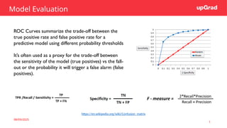
Model Evaluation
ROC Curves summarize the trade-off between the
true positive rate and false positive rate for a
predictive model using different probability thresholds
It’s often used as a proxy for the trade-off between
the sensitivity of the model (true positives) vs the fall-
out or the probability it will trigger a false alarm (false
positives).
https://en.wikipedia.org/wiki/Confusion_matrix

08/09/2025 2
Cross Validation
Cross-validation is a resampling technique
used to evaluate machine learning models on
a limited data set.
The most common use of cross-validation is
the k-fold cross-validation method. Our
training set is split into K partitions, the model
is trained on K-1 partitions and the test error
is predicted and computed on
the Kth partition. This is repeated for each
unique group and the test errors are
averaged across.

08/09/2025 3
Decision Tree
Decision tree is the most powerful and
popular tool for classification and
prediction. A Decision tree is a flowchart
like tree structure, where each internal
node denotes a test on an attribute,
each branch represents an outcome of
the test, and each leaf node (terminal
node) holds a class label.

08/09/2025 5
When to stop splitting?
As a problem usually has a large set of features, it results in large number of split, which in turn gives a
huge tree. Such trees are complex and can lead to overfitting.
Pruning
Remove the branches that make use of
features having low importance.This
way, we reduce the complexity of tree, and
thus increasing its predictive power by
reducing overfitting.
Truncation
Stop the tree wile it is still growing so that it
may not end up with leaves containing vary
less data-points, one way to do this is by
setting the minimum number

Click to add Title
08/09/2025 Footer
Practice in teams of 4 students
Industry expert mentoring to learn better
Get personalised feedback for improvements
6
Poll 4
08-09-2025 11
Question: we want to segregate the students based on target variable (playing
cricket or not).we split the population using input variables Gender find the
homogeneity of sub-nodes using Gini.
A) 0.51
B) 0.59
C) 0.33
D) 0.49

Click to add Title
08/09/2025 Footer
7
Poll 4 (Solution)
08-09-2025 11
Question: we want to segregate the students based on target variable (playing
cricket or not).we split the population using input variables Gender find the
homogeneity of sub-nodes using Gini.
A) 0.51
B) 0.59
C) 0.33
D) 0.49
Calculate, Gini for sub-node Female = (0.2)*(0.2)+(0.8)*(0.8)=0.68
Gini for sub-node Male = (0.65)*(0.65)+(0.35)*(0.35)=0.55
Calculate weighted Gini for Split Gender = (10/30)*0.68+(20/30)*0.55 = 0.59

08/09/2025 8
What is the curse of dimensionality?
Sparsity of data occurs when moving to higher
dimensions. the volume of the space represented
grows so quickly that the data cannot keep up and
thus becomes sparse
The second issue that arises is related to sorting or classifying
the data. In low dimensional spaces, data may seem very
similar but the higher the dimension the data points may seem
far.
Infinite Features Requires Infinite Training
A careful choice of the number of dimensions (features) to be used is
the prerogative of the data scientist training the Model

08/09/2025 9
What is Principal Components Analysis?
Principal Components Analysis is an unsupervised
learning class of statistical techniques used to
explain data in high dimension using smaller
number of variables called the principal
components.
The loading vector Ф1 with elements Ф11, Ф21,…,Фp1 defines a direction in the feature space along which there
is maximum variance in the data.
Thus, if we are to project the n data points x1, x2,…, xn
onto this direction, then projected values are the actual principal component scores z11, z21, …, zn1.
After the first principal components, Z1 of the features has been determined, then the second principal
component is the linear combination of X1, ,X2,… Xp that has the highest variance out of all the linear
combinations that are uncorrelated with Z1. The second principal component scores z12, z22,…,zn2 take the
form

Bias and Variance in regression models
The prediction error for any machine learning
algorithm can be broken down into three parts:
• Bias Error
• Variance Error
• Irreducible Error
The irreducible error cannot be reduced regardless
of what algorithm is used. It is the error introduced
from the chosen framing of the problem and may be
caused by factors like unknown variables that
influence the mapping of the input variables to the
output variable.
• Low Bias: Suggests less assumptions about the form of the target function.
• High-Bias: Suggests more assumptions about the form of the target function.
• Low Variance: Suggests small changes to the estimate of the target function with changes to the training
dataset.
• High Variance: Suggests large changes to the estimate of the target function with changes to the training
dataset.

Bias-Variance Trade-Off
The goal of any supervised machine learning algorithm is to achieve low bias and low variance. In
turn the algorithm should achieve good prediction performance.
• Parametric or linear machine learning algorithms
often have a high bias but a low variance.
• Non-parametric or non-linear machine learning
algorithms often have a low bias but a high
variance.
The parameterization of machine learning algorithms is often a battle to balance out bias and
variance.

08/09/2025 12
Regularized Linear Regression
One of the major aspects of training your
machine learning model is avoiding
overfitting. The model will have a low accuracy if
it is overfitting. This happens because your
model is trying too hard to capture the noise
in your training dataset.
Regularization
This is a form of regression, that constrains/ regularizes or shrinks the
coefficient estimates towards zero. In other words, this technique
discourages learning a more complex or flexible model, so as to avoid
the risk of overfitting.

08/09/2025 13
Ridge Regression
RSS is modified by adding the shrinkage quantity.
Now, the coefficients are estimated by minimizing this function. Here, is
λ
the tuning parameter that decides how much we want to penalize the
flexibility of our model.
The increase in flexibility of a model is represented by increase in its
coefficients, and if we want to minimize the above function, then these
coefficients need to be small.

08/09/2025 14
Lasso Regression
Lasso is another variation, in which the above
function is minimized. Its clear that
this variation differs from ridge regression
only in penalizing the high coefficients.

08/09/2025 15
Regularized Linear Regression
The ridge regression is expressed by β1² + β2² s
≤ . This
implies that ridge regression coefficients have the smallest
RSS(loss function) for all points that lie within the circle
given by β1² + β2² s
≤
The lasso, the equation becomes,|β1|+|β2| s
≤ .
This implies that lasso coefficients have the smallest
RSS(loss function) for all points that lie within the
diamond given by |β1|+|β2| s.
≤

08/09/2025
16
Model Evaluation
A confusion matrix shows the number of correct
and incorrect predictions made by the classification
model compared to the actual outcomes (target
value) in the data. The matrix is NxN, where N is the
number of target values (classes). Performance of
such models is commonly evaluated using the data
in the matrix. The following table displays a 2x2
confusion matrix for two classes (Positive and
Negative).
Confusion Matrix
Target
Positive Negative
Positive a b Positive Predictive
Value
a/(a+b)
Negative c d
Negative Predictive
Value
d/(c+d)
Sensitivity Specificity Accuracy = (a+d)/(a+b+c+d)
•Accuracy : the proportion of the total number of predictions that were correct.
•Positive Predictive Value or Precision : the proportion of positive cases that were correctly identified.
•Negative Predictive Value : the proportion of negative cases that were correctly identified.
•Sensitivity or Recall : the proportion of actual positive cases which are correctly identified.
•Specificity : the proportion of actual negative cases which are correctly identified.

08/09/2025 18
PCA is useful when you have a large number of potentially correlated variables. Also, PCA can
be used to visualize complex datasets.
PCA
We saw that if each row in the original dataset A (m x n) represents a user and each column an
item such as a book, then:
•The matrix U (m x k) maps the users to the new k themes/latent variables
•The diagonal matrix S (k x k) represents the strength of each feature
• Matrix V' (k x n) maps each of the k themes/latent variables to the original n features.

Click to add Title
08/09/2025 Footer
18
250000011100
Poll 5
08-09-2025 11
What are the PC1 and PC2 values for
given x=3 and y=2 ?
A) 3.4 & 1.2
B) 3.6 & -0.2
C) 3.4 & -0.2
D) 3.6 & 1.2

Click to add Title
08/09/2025 Footer
19
Poll 5 (Answer)
08-09-2025 11
What are the PC1 and PC2 values for
given x=3 and y=2 ?
A) 3.4 & 1.2
B) 3.6 & -0.2
C) 3.4 & -0.2
D) 3.6 & 1.2

08/09/2025 19
K-Mean Clustering
• The number of clusters that you want to divide your data points into, i.e. the value of K has to be pre-
determined.
• The choice of the initial cluster centers can have an impact on the final cluster formation.
• The clustering process is very sensitive to the presence of outliers in the data.
• Since the distance metric used in the clustering process is the Euclidean distance, you need to bring all your
attributes on the same scale. This can be achieved through standardization.
• The K-Means algorithm does not work with categorical data.
Choosing the number of clusters K
Elbow method
• Compute clustering algorithm (e.g., k-means clustering) for different values of k. For instance, by varying k from 1 to 10
clusters.
• For each k, calculate the total within-cluster sum of square (wss)
• Plot the curve of wss according to the number of clusters k.
• The location of a bend (knee) in the plot is generally considered as an indicator of the appropriate number of clusters.
CLUSTERING

08/09/2025 20
Hierarchical Clustering algorithm
Given a set of N items to be clustered, the steps in the hierarchical clustering are:
• Calculate the NxN distance (similarity) matrix, which calculates the distance of each data point from the
other.
• Start by assigning each item to its own cluster, so that if you have N items, you now have N clusters, each
containing just one item.
• Find the closest (most similar) pair of clusters and merge them into a single cluster, so that now you have one less cluster.
• Compute distances (similarities) between the new cluster and each of the old clusters.
• Repeat steps 3 and 4 until all items are clustered into a single cluster of size N
Single Linkage
Here, the distance between 2 clusters is defined as the shortest distance between points in the two clusters
Complete Linkage
Here, the distance between 2 clusters is defined as the maximum distance between any 2 points in the clusters
Average Linkage
Here, the distance between 2 clusters is defined as the average distance between every point of one cluster to every other point
of the other cluster.
CLUSTERING

Click to add Title
08/09/2025 Footer
22
Poll 6
08-09-2025 11
Which of the following clustering
representations and dendrogram depicts the
use of MIN or Single link proximity function in
hierarchical clustering?
(A) (B) (C)
Distance Matrix

Click to add Title
08/09/2025 Footer
23
Poll 6 (Answer)
08-09-2025 11
Which of the following clustering
representations and dendrogram depicts the
use of Single link proximity function in
hierarchical clustering?
(A) (B) (C)
Distance Matrix

Click to add Title
08/09/2025 Footer
24
Poll 7
08-09-2025 11
What is the most appropriate no. of clusters for the
data points represented by the following
dendrogram?
A. 2
B. 4
C. 6
D. 8

Click to add Title
08/09/2025 Footer
25
Poll 7 (Answer)
08-09-2025 11
What is the most appropriate no. of clusters for the
data points represented by the following
dendrogram?
A. 2
B. 4
C. 6
D. 8

08/09/2025 26
Ensemble methods
Ensemble learning is a machine
learning paradigm where
multiple models (often called
“weak learners”) are trained to
solve the same problem and
combined to get better results.
https://towardsdatascience.com/ensemble-methods-bagging-boosting-and-stacking-c9214a10a205

08/09/2025 27
Bagging
Bagging, that often considers
homogeneous weak learners,
learns them independently
from each other in parallel and
combines them following some
kind of deterministic averaging
process
https://learn.upgrad.com/v/course/515/session/77070/segment/431269

08/09/2025 28
Random Forest
Random forest, like its name implies,
consists of a large number of individual
decision trees that operate as
an ensemble. Each individual tree in the
random forest spits out a class
prediction and the class with the most
votes becomes our model’s prediction
The reason for this wonderful effect is
that the trees protect each other from
their individual errors (as long as they
don’t constantly all err in the same
direction)

08/09/2025 29
Random Forest
Bagging (Bootstrap Aggregation) — Decision trees are very sensitive to the
data they are trained on — small changes to the training set can result in
significantly different tree structures. Random forest takes advantage of this by
allowing each individual tree to randomly sample from the dataset with
replacement, resulting in different trees.
Feature Randomness — In a normal decision
tree, while splitting a node, we consider all the
features and pick the one that produces the
most separation. In contrast, each tree in a
random forest can pick only from a random
subset of features. This forces even more
variation amongst the trees in the model and
ultimately results in lower correlation across
trees and more diversification.

08/09/2025 30
Different ensemble methods
Boosting, that often considers homogeneous weak learners, learns them sequentially in a very adaptive way (a base model depends
on the previous ones) and combines them following a deterministic strategy
https://medium.com/mlreview/gradient-boosting-from-scratch-1e317ae4587d
Base model is
created on a subset
The observations
which are incorrectly
predicted, are given
higher weights and
an another model is
created and
predictions are made
on the dataset
multiple models are created, each correcting
the errors of the previous model.
The final model (strong learner)
. The individual models would not
perform well on the entire dataset,
but they work well for some part of
the dataset. Thus, each model
actually boosts the performance of
the ensemble.

08/09/2025 31
Gradient Descent
Gradient descent is an optimization algorithm used to
minimize some function by iteratively moving in the
direction of steepest descent as defined by the negative
of the gradient
While the direction of the gradient tells us which
direction has the steepest ascent, it's magnitude tells
us how steep the steepest ascent/descent is. So, at the
minima, where the contour is almost flat, you would
expect the gradient to be almost zero. In fact, it's
precisely zero for the point of minima.

08/09/2025 32
Gradient Descent
In practice, we might never exactly reach the minima, but we keep oscillating in a flat region in
close vicinity of the minima. As we oscillate our this region, the loss is almost the minimum we
can achieve, and doesn't change much as we just keep bouncing around the actual minimum.
Often, we stop our iterations when the loss values haven't improved in a pre-decided number,
say, 10, or 20 iterations. When such a thing happens, we say our training has converged, or
convergence has taken place.

08/09/2025 40
What & Why of Overfitting and Underfitting
Overfitting refers to a model that models the training data too
well.
Overfitting happens when a model learns the detail and noise
in the training data to the extent that it negatively impacts the
performance of the model on new data. This means that the
noise or random fluctuations in the training data is picked up
and learned as concepts by the model. The problem is that
these concepts do not apply to new data and negatively
impact the models ability to generalize.
Underfitting refers to a model that can neither model the training data nor generalize to new data.
An underfit machine learning model is not a suitable model and will be obvious as it will have poor performance
on the training data.

08/09/2025 41
What & Why of Overfitting and Underfitting
Underfitting Overfitting
Good-Fit

08/09/2025 42
How to Detect Overfitting?
Detecting overfitting is almost impossible before you test the data. It can help address the inherent
characteristic of overfitting, which is the inability to generalize data sets. The data can, therefore, be
separated into different subsets to make it easy for training and testing. The data is split into three main
parts, i.e., a train set ,a test set & a validate set
By segmenting the dataset, we can examine the performance of the model on each set of
data to spot overfitting when it occurs. The performance can be measured using the
percentage of accuracy observed in train & validate data sets to conclude on the presence
of overfitting.
– Training set: A set of examples used for learning, that
is to fit the parameters of the classifier.
– Validation set: A set of examples used to tune the
parameters of a classifier, for example to choose the
number of hidden units in a neural network.
– Test set: A set of examples used only to assess the
performance of a fully-specified classifier.

Click to add Title
08/09/2025 Footer
43
Poll 1
08-09-2025 11
How does number of observations influence overfitting? Choose the correct answer(s)
1. In case of fewer observations, it is easy to overfit the data.
2. In case of fewer observations, it is hard to overfit the data.
3. In case of more observations, it is easy to overfit the data.
4. In case of more observations, it is hard to overfit the data
A. 1 and 4
B. 2 and 3
C. 1 and 3
D. None of theses

Click to add Title
08/09/2025 Footer
44
Poll 1
08-09-2025 11
How does number of observations influence overfitting? Choose the correct answer(s)
1. In case of fewer observations, it is easy to overfit the data.
2. In case of fewer observations, it is hard to overfit the data.
3. In case of more observations, it is easy to overfit the data.
4. In case of more observations, it is hard to overfit the data
A. 1 and 4
B. 2 and 3
C. 1 and 3
D. None of theses

08/09/2025
Thank You!
#LifeKoKaroLift
21

machinelearningpresentationon machine .pptx

More Related Content

Similar to machinelearningpresentationon machine .pptx

Recently uploaded

machinelearningpresentationon machine .pptx