Download to read offline
![SGD in ERM – mini batch SGD
To solve empirical risk minimization (ERM)
f (θ) =
1
n
n
i=1
fi (θ),
where fi (θ) = θ(Zi ).
At each step:
Draw S i.i.d. uniformly random indices It from [n] (with
replacement)
Compute stochastic gradient gs(θt) = 1
S i∈It
fi (θt)
θt+1 = θt − ηgs(θt)](https://image.slidesharecdn.com/44constantine-dstop-2018-181128221033/75/Statistical-Inference-Using-Stochastic-Gradient-Descent-5-2048.jpg)
![Asymptotic normality – classical results
M-estimator – statistics
When number of samples n → ∞,
√
n(θ − θ∗
) N(0, H∗−1
G∗
H∗−1
),
where G∗ = EZ [ θ θ∗ (Z) θ θ∗ (Z) ] and H∗ = EZ [ 2
θ θ∗ (Z)].
Stochastic approximation – optimization
When number of steps t → ∞,
√
t
1
t
t
i=1
θt − θ N(0, H−1
GH−1
),
where G = E[gs(θ)gs(θ) |= θ] and H = 2f (θ).](https://image.slidesharecdn.com/44constantine-dstop-2018-181128221033/75/Statistical-Inference-Using-Stochastic-Gradient-Descent-6-2048.jpg)
![Asymptotic normality – classical results
M-estimator – statistics
When number of samples n → ∞,
√
n(θ − θ∗
) N(0, H∗−1
G∗
H∗−1
),
where G∗ = EZ [ θ θ∗ (Z) θ θ∗ (Z) ] and H∗ = EZ [ 2
θ θ∗ (Z)].
Stochastic approximation – optimization
When number of steps t → ∞,
√
t
1
t
t
i=1
θt − θ N(0, H−1
GH−1
),
where G = E[gs(θ)gs(θ) |= θ] and H = 2f (θ).
SGD not only useful for optimization,
but also useful for statistical inference!](https://image.slidesharecdn.com/44constantine-dstop-2018-181128221033/75/Statistical-Inference-Using-Stochastic-Gradient-Descent-7-2048.jpg)
![Statistical inference using mini batch SGD
burn in
θ−b, θ−b+1, · · · θ−1, θ0,
¯θ
(i)
t =1
t
t
j=1 θ
(i)
j
θ
(1)
1 , θ
(1)
2 , · · · , θ
(1)
t
discarded
θ
(1)
t+1, θ
(1)
t+2, · · · , θ
(1)
t+d
θ
(2)
1 , θ
(2)
2 , · · · , θ
(2)
t θ
(2)
t+1, θ
(2)
t+2, · · · , θ
(2)
t+d
...
θ
(R)
1 , θ
(R)
2 , · · · , θ
(R)
t θ
(R)
t+1, θ
(R)
t+2, · · · , θ
(R)
t+d
At each step:
Draw S i.i.d. uniformly random
indices It from [n] (with replacement)
Compute stochastic gradient
gs(θt) = 1
S i∈It
fi (θt)
θt+1 = θt − ηgs(θt)
Use an ensemble of i = 1, 2, . . . , R estima-
tors for statistical inference:
θ(i)
= θ +
√
S
√
t
√
n
(¯θ
(i)
t − θ).](https://image.slidesharecdn.com/44constantine-dstop-2018-181128221033/75/Statistical-Inference-Using-Stochastic-Gradient-Descent-8-2048.jpg)
![Theoretical guarantee
Theorem
For a differentiable convex function f (θ) = 1
n
n
i=1 fi (θ), with gradient f (θ), let θ ∈ Rp be
its minimizer, and denote its Hessian at θ by H := 2f (θ) . Assume that ∀θ ∈ Rp, f satisfies:
(F1) Weak strong convexity: (θ − θ) f (θ) ≥ α θ − θ 2
2, for constant α > 0,
(F2) Lipschitz gradient continuity: f (θ) 2 ≤ L θ − θ 2, for constant L > 0,
(F3) Bounded Taylor remainder: f (θ) − H(θ − θ) 2 ≤ E θ − θ 2
2, for constant E > 0,
(F4) Bounded Hessian spectrum at θ: 0 < λL ≤ λi (H) ≤ λU < ∞, ∀i.
Furthermore, let gs(θ) be a stochastic gradient of f , satisfying:
(G1) E [gs(θ) | θ] = f (θ),
(G2) E gs(θ) 2
2 | θ ≤ A θ − θ 2
2 + B,
(G3) E gs(θ) 4
2 | θ ≤ C θ − θ 4
2 + D,
(G4) E gs(θ)gs(θ) | θ − G 2
≤ A1 θ − θ 2 + A2 θ − θ 2
2 + A3 θ − θ 3
2 + A4 θ − θ 4
2,
for positive, data dependent constants A, B, C, D, Ai , for i = 1, . . . , 4. Assume that
θ1 − θ 2
2 = O(η); then for sufficiently small step size η > 0, the average SGD sequence
θt = 1
t
n
i=1 θi satisfies:
tE[(¯θt − θ)(¯θt − θ) ] − H−1
GH−1
2
√
η + 1
tη + tη2,
where G = E[gs(θ)gs(θ) | θ].](https://image.slidesharecdn.com/44constantine-dstop-2018-181128221033/75/Statistical-Inference-Using-Stochastic-Gradient-Descent-13-2048.jpg)
![Theoretical guarantee
Theorem
For a differentiable convex function f (θ) = 1
n
n
i=1 fi (θ), with gradient f (θ), let θ ∈ Rp be
its minimizer, and denote its Hessian at θ by H := 2f (θ) . Assume that ∀θ ∈ Rp, f satisfies:
(F1) Weak strong convexity: (θ − θ) f (θ) ≥ α θ − θ 2
2, for constant α > 0,
(F2) Lipschitz gradient continuity: f (θ) 2 ≤ L θ − θ 2, for constant L > 0,
(F3) Bounded Taylor remainder: f (θ) − H(θ − θ) 2 ≤ E θ − θ 2
2, for constant E > 0,
(F4) Bounded Hessian spectrum at θ: 0 < λL ≤ λi (H) ≤ λU < ∞, ∀i.
Furthermore, let gs(θ) be a stochastic gradient of f , satisfying:
(G1) E [gs(θ) | θ] = f (θ),
(G2) E gs(θ) 2
2 | θ ≤ A θ − θ 2
2 + B,
(G3) E gs(θ) 4
2 | θ ≤ C θ − θ 4
2 + D,
(G4) E gs(θ)gs(θ) | θ − G 2
≤ A1 θ − θ 2 + A2 θ − θ 2
2 + A3 θ − θ 3
2 + A4 θ − θ 4
2,
for positive, data dependent constants A, B, C, D, Ai , for i = 1, . . . , 4. Assume that
θ1 − θ 2
2 = O(η); then for sufficiently small step size η > 0, the average SGD sequence
θt = 1
t
n
i=1 θi satisfies:
tE[(¯θt − θ)(¯θt − θ) ] − H−1
GH−1
2
√
η + 1
tη + tη2,
where G = E[gs(θ)gs(θ) | θ].
Proof idea: H−1 = η i≥0(I − ηH)i](https://image.slidesharecdn.com/44constantine-dstop-2018-181128221033/75/Statistical-Inference-Using-Stochastic-Gradient-Descent-14-2048.jpg)
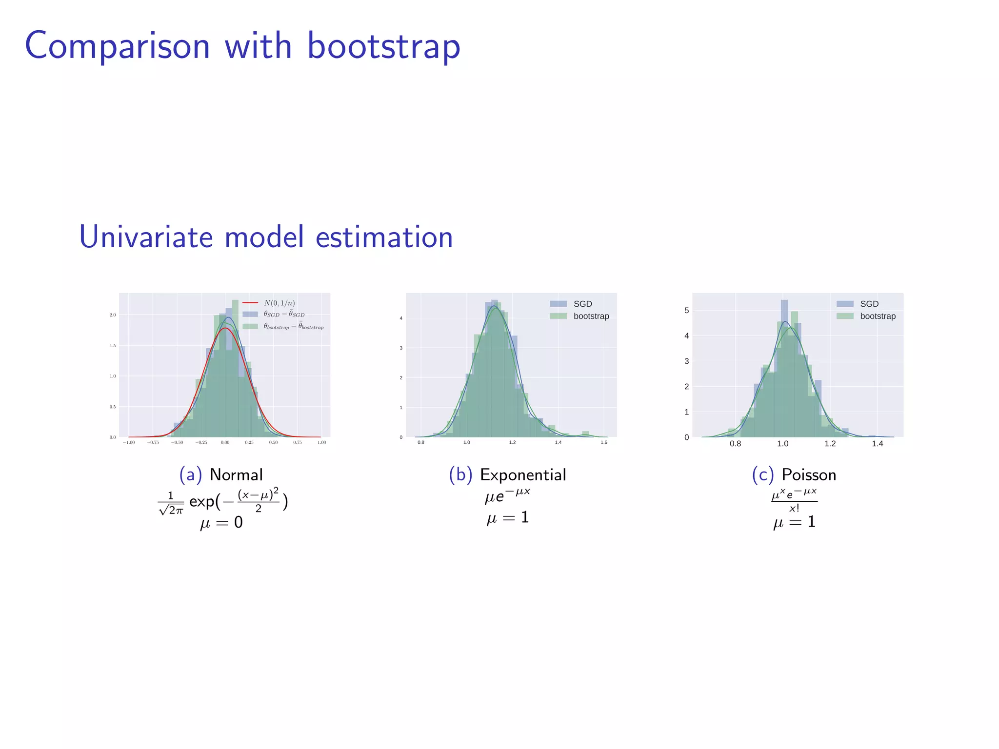
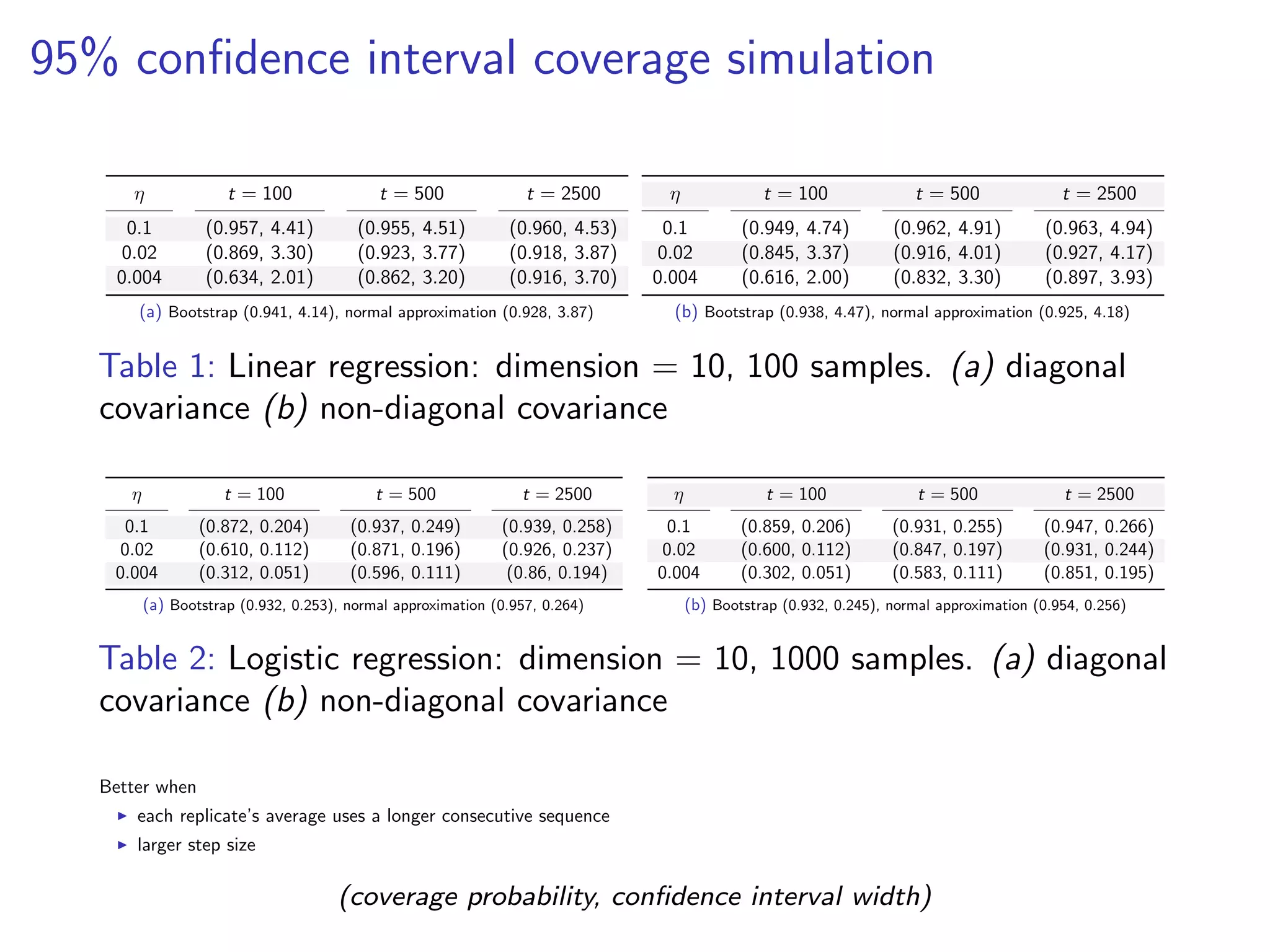
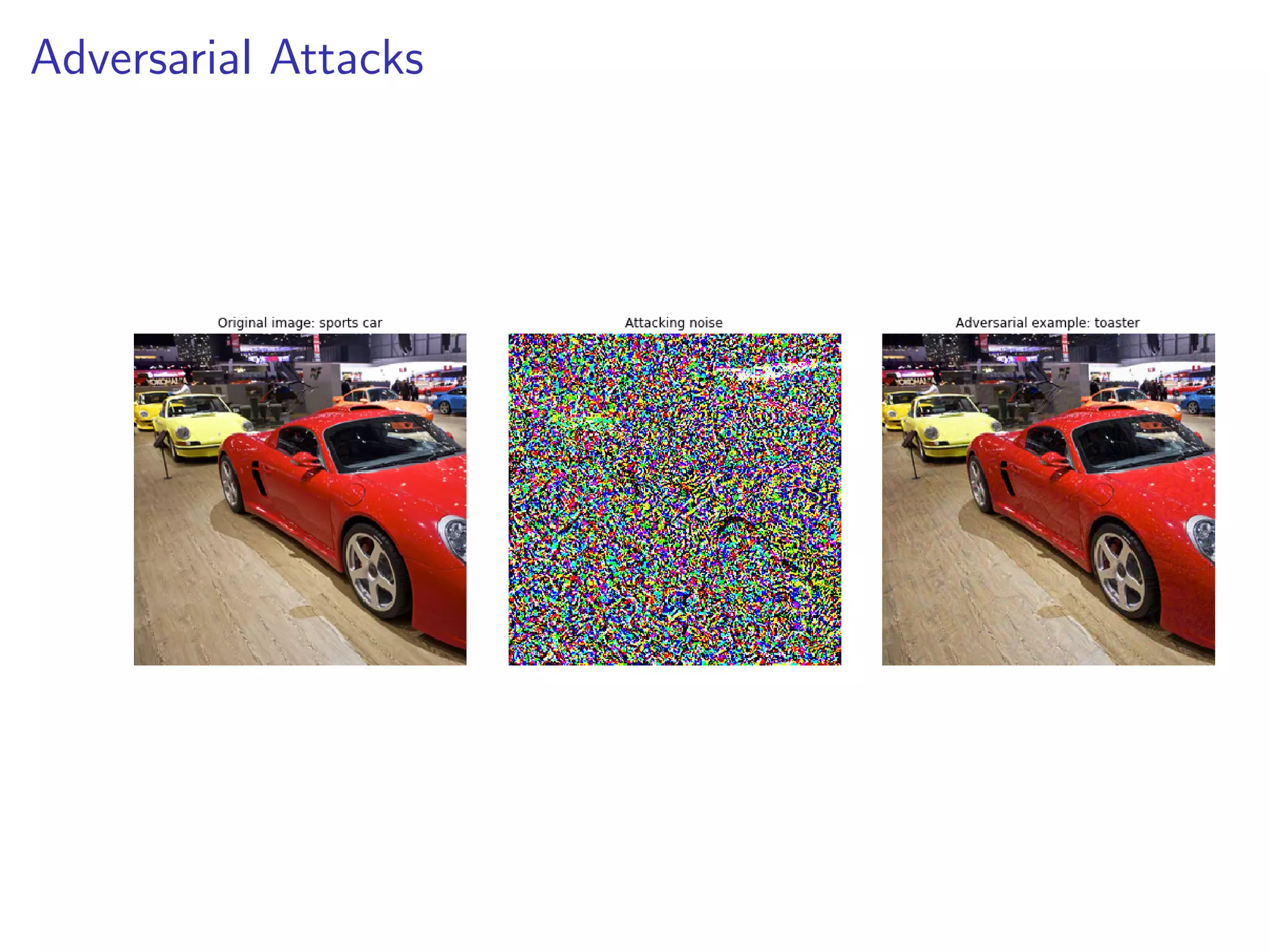
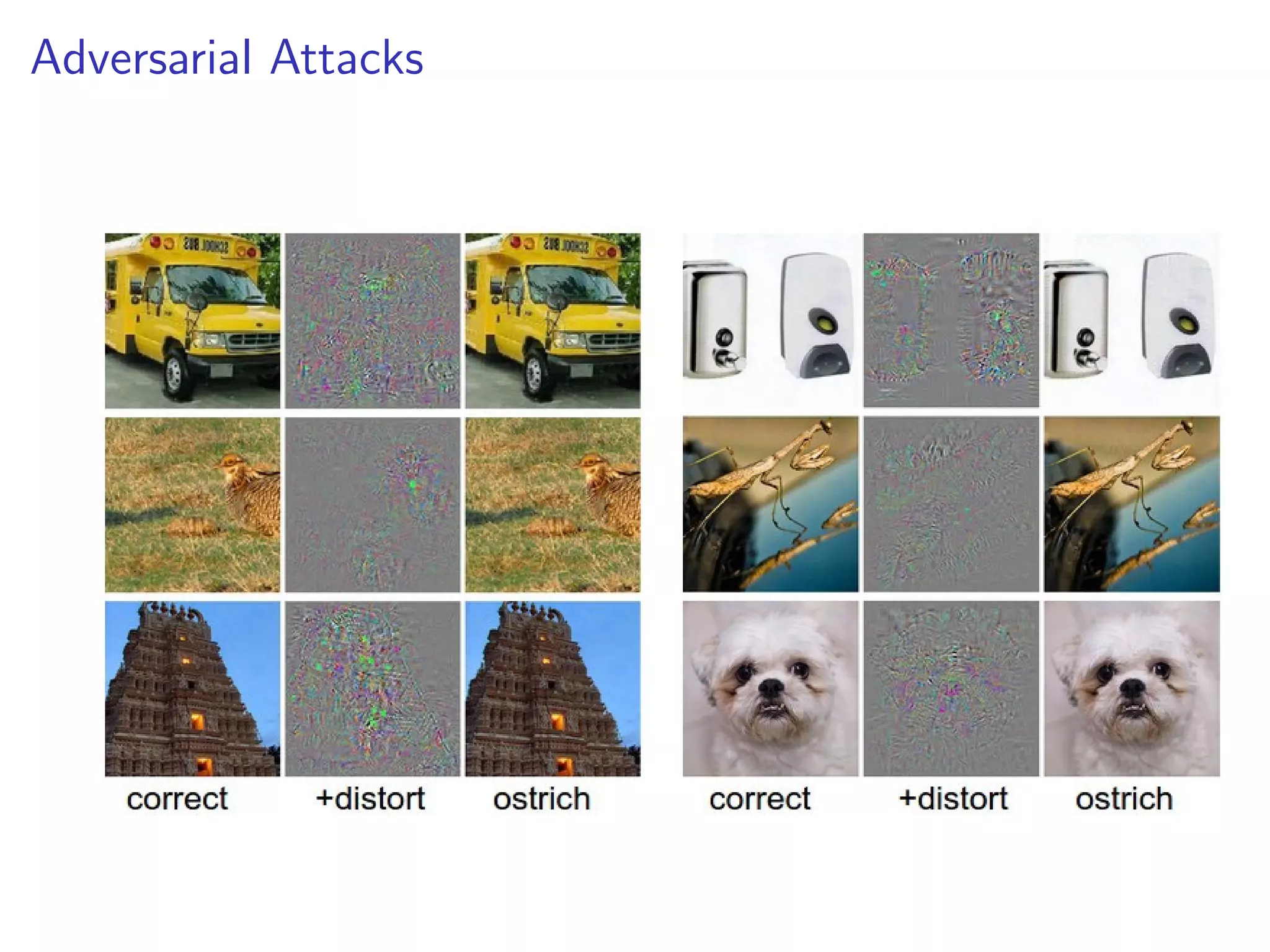
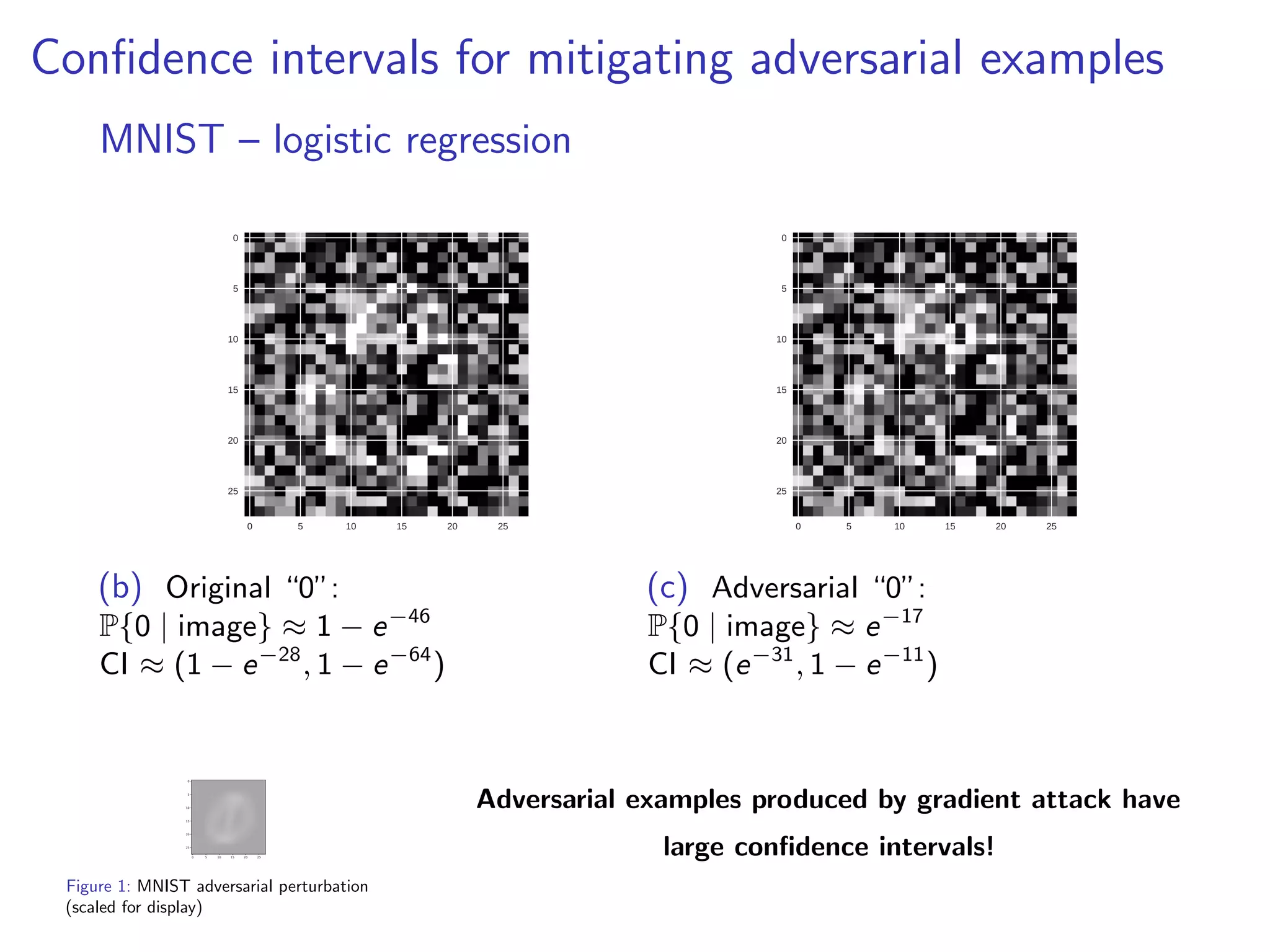
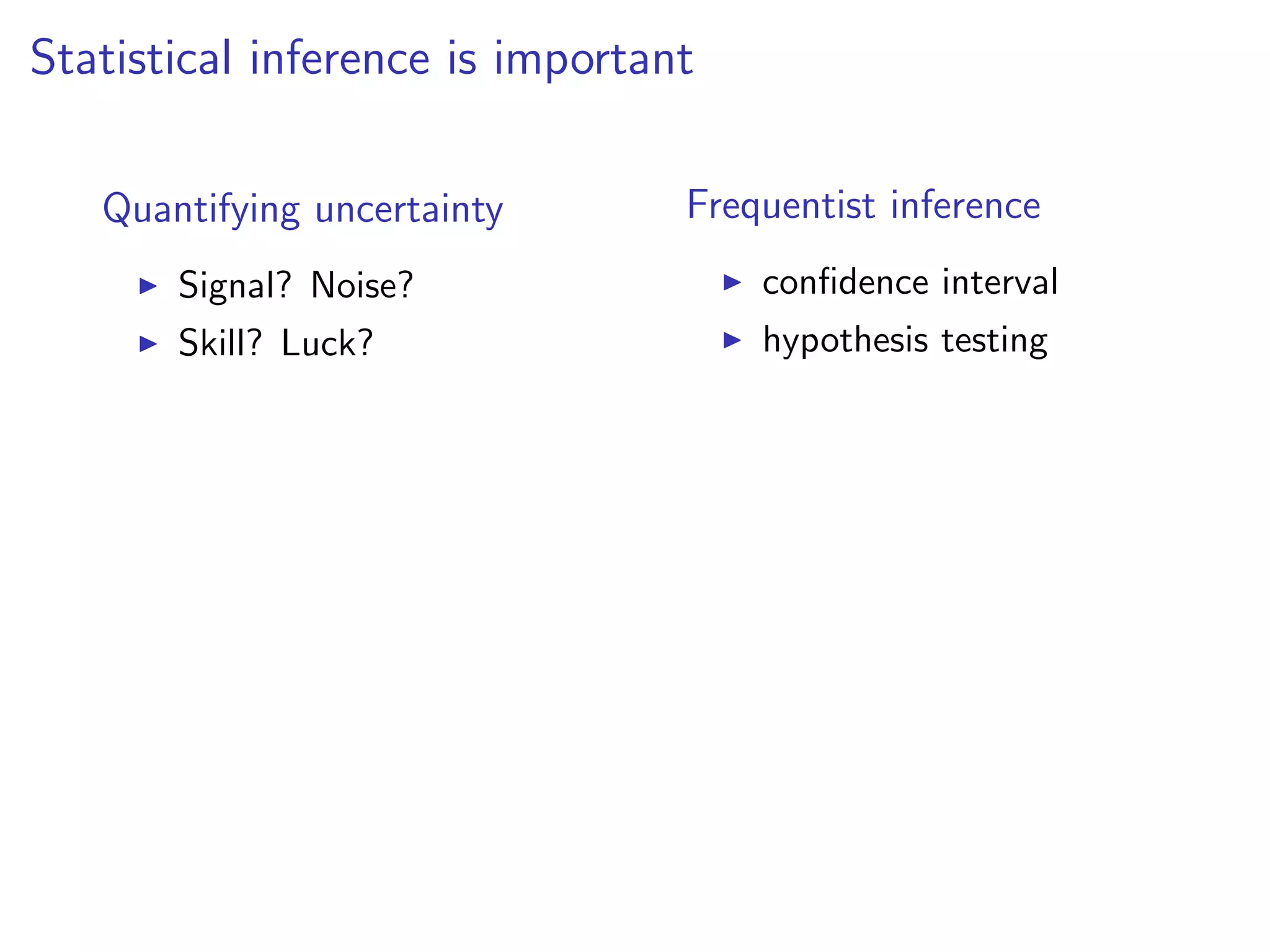
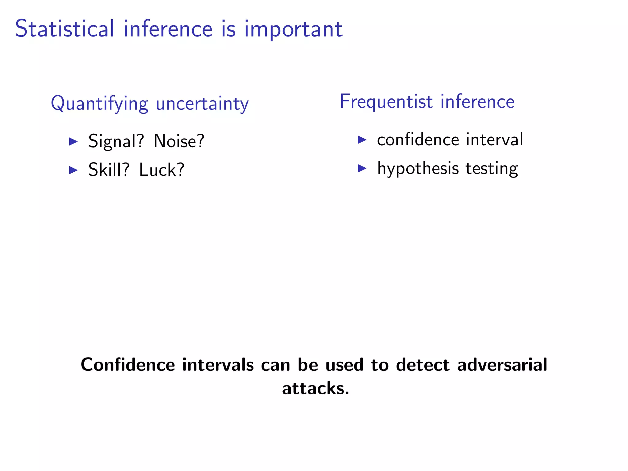
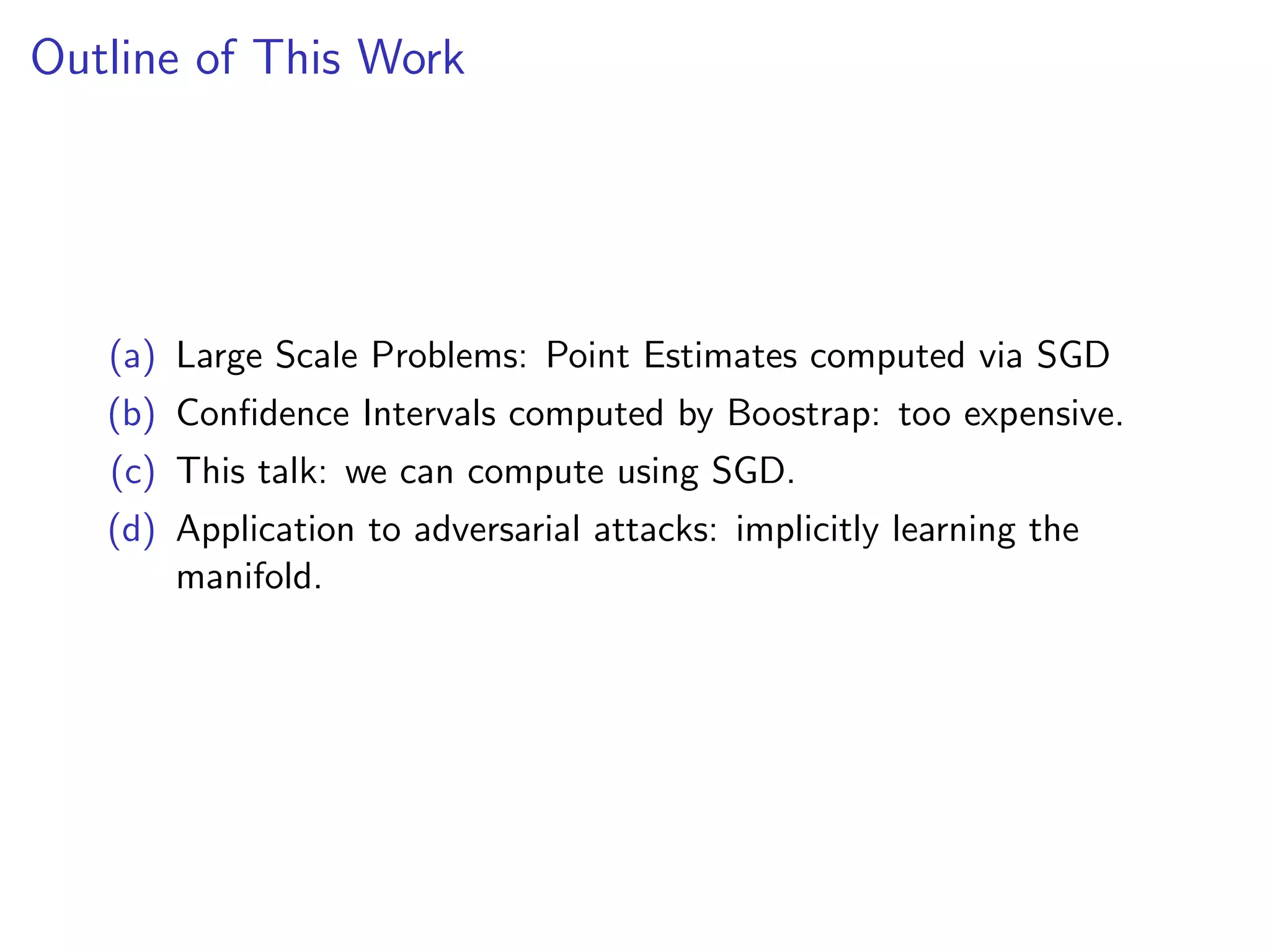
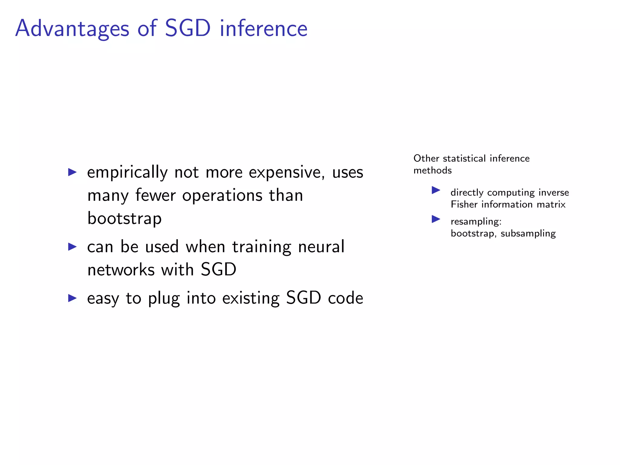
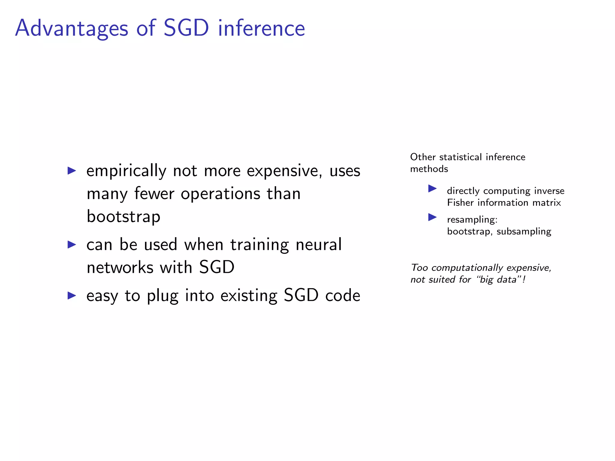
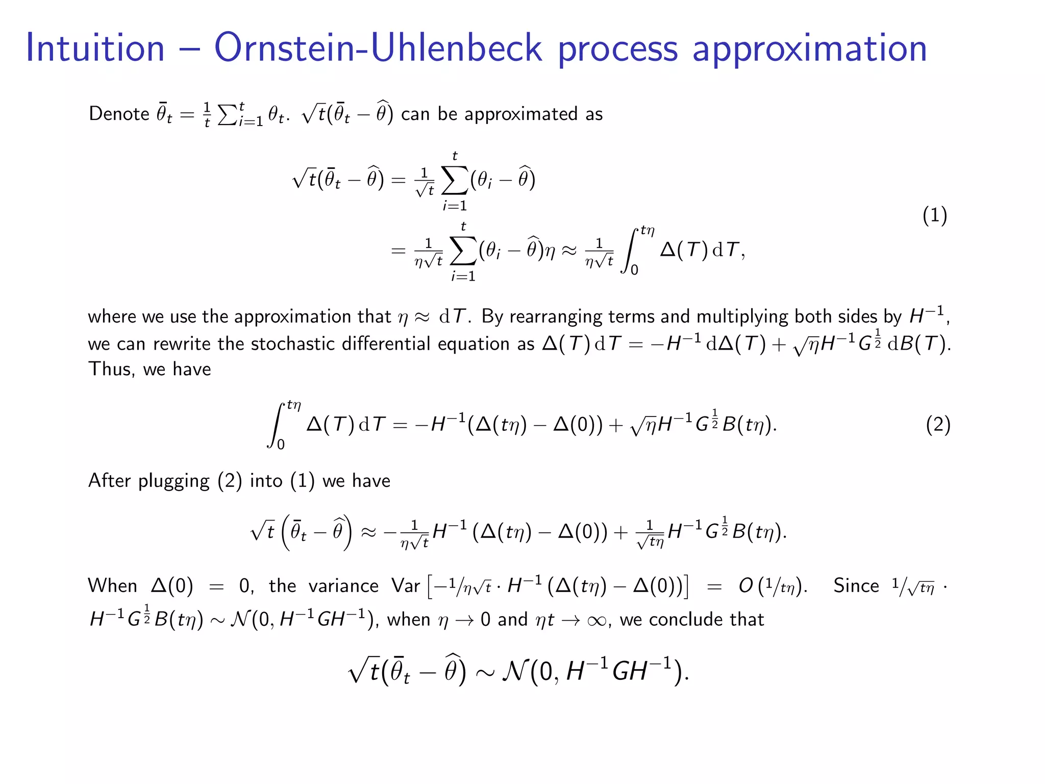
This document discusses the application of stochastic gradient descent (SGD) for statistical inference, particularly in the context of detecting adversarial attacks in machine learning. It outlines how confidence intervals can be computed using SGD, which is more efficient than traditional bootstrap methods for large data problems. The work emphasizes the practical advantages of using SGD for both inference and optimization in statistical analysis.


![[ICLR2021 (spotlight)] Benefit of deep learning with non-convex noisy gradien...](https://cdn.slidesharecdn.com/ss_thumbnails/iclr2021-210331133549-thumbnail.jpg?width=640&height=640&fit=bounds)