
Download to read offline


![Based on Land Mobile Satellite Channel
Model [1].
LOS: interaction with buildings, trees, poles
NLOS echoes: stochastic
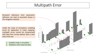
Geometric echoes: reflective, persistent
1. Simulate multipath echoes
2. Scalar tracking with narrow correlator
3. Navigation filter (EKF)
Naïve receiver: persistent biases after 100
sessions
Ideal NLOS rejection: accept signals with at
least 10 dB LOS advantage
Realistic receiver with normalized
innovation test based NLOS exclusion](https://image.slidesharecdn.com/06humphreysapril18-180626034311/85/Collaborative-Sensing-for-Automated-Vehicles-24-320.jpg)
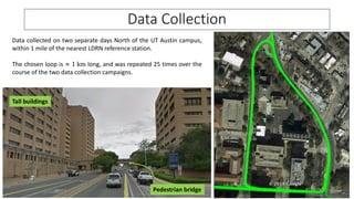
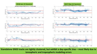
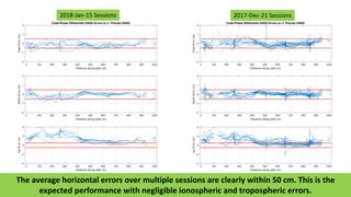
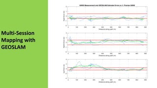

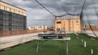

The document discusses the development of collaborative sensing systems for automated vehicles to address blind spots using 5G technology, enhancing safety in automated driving. It highlights the potential of vehicle-to-vehicle and vehicle-to-infrastructure connectivity to share sensor data, improving situational awareness and reducing collision risks. The document also details experimental setups and findings related to collaborative mapping and GNSS error assessments, ultimately aiming for high-resolution mapping capabilities in urban environments.


