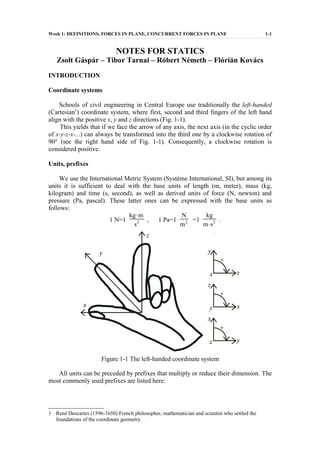
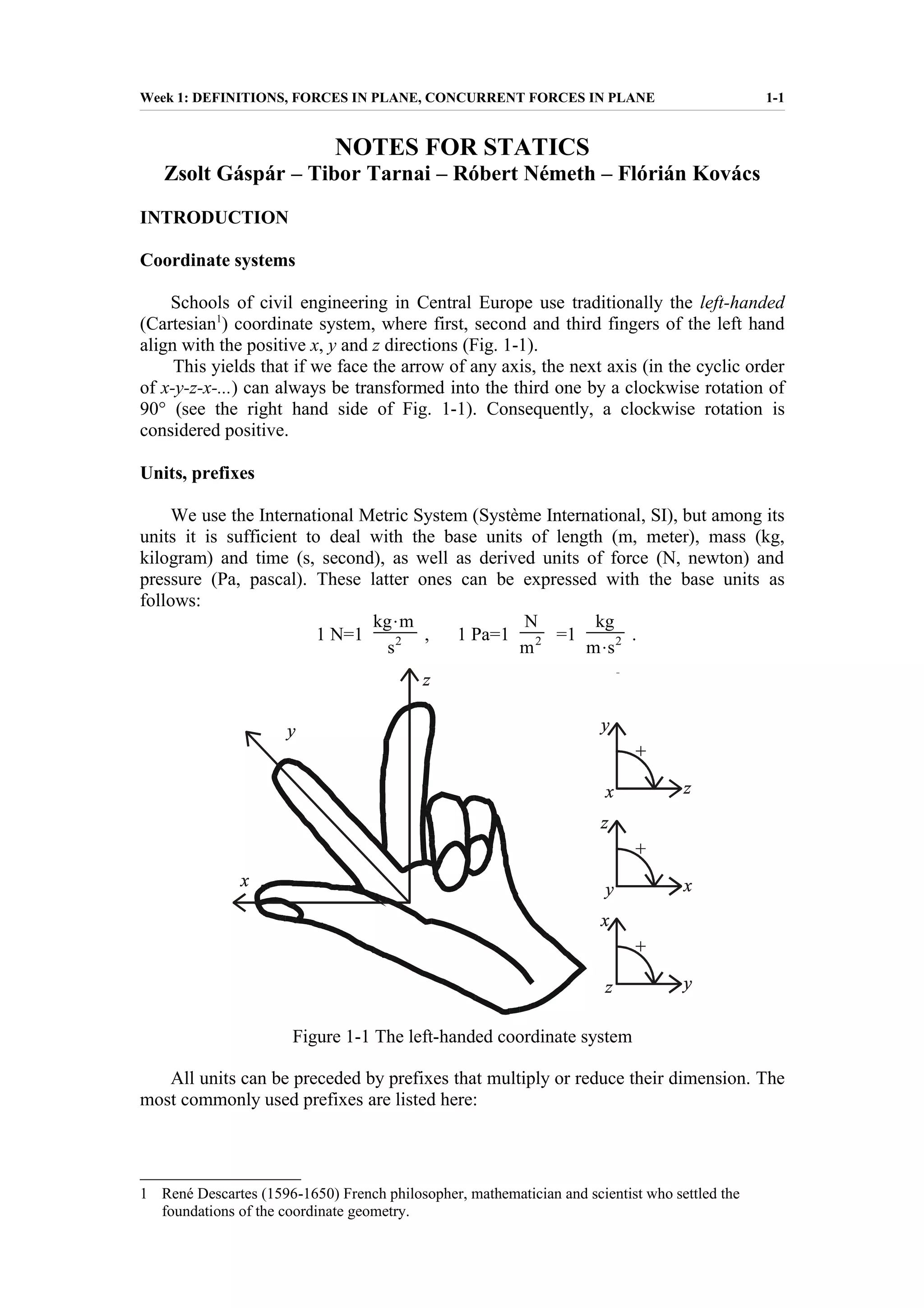
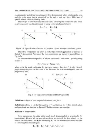
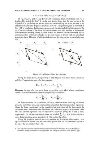
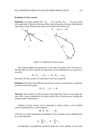
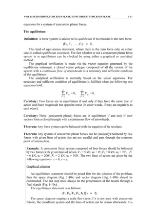
Text Book: An Introduction to Mechanics by Kleppner and Kolenkow
Chapter 1: Vectors and Kinematics
-Explain the concept of vectors.
-Explain the concepts of position, velocity and acceleration for different kinds of motion.
References:
Halliday, Resnick and Walker
Berkley Physics Volume-1
3-1 VECTORS AND THEIR COMPONENTS
After reading this module, you should be able to . . .
3.01 Add vectors by drawing them in head-to-tail arrangements, applying the commutative and associative laws.
3.02 Subtract a vector from a second one.
3.03 Calculate the components of a vector on a given coordinate system, showing them in a drawing.
3.04 Given the components of a vector, draw the vector
and determine its magnitude and orientation.
3.05 Convert angle measures between degrees and radians.
3-2 UNIT VECTORS, ADDING VECTORS BY COMPONENTS
After reading this module, you should be able to . . .
3.06 Convert a vector between magnitude-angle and unit vector notations.
3.07 Add and subtract vectors in magnitude-angle notation
and in unit-vector notation.
3.08 Identify that, for a given vector, rotating the coordinate
system about the origin can change the vector’s components but not the vector itself.
etc...
Fundamentals of Physics "MOTION IN TWO AND THREE DIMENSIONS"Muhammad Faizan Musa
4-1 POSITION AND DISPLACEMENT
After reading this module, you should be able to . . .
4.01 Draw two-dimensional and three-dimensional position
vectors for a particle, indicating the components along the
axes of a coordinate system.
4.02 On a coordinate system, determine the direction and
magnitude of a particle’s position vector from its components, and vice versa.
4.03 Apply the relationship between a particle’s displacement vector and its initial and final position vectors.
4-2 AVERAGE VELOCITY AND INSTANTANEOUS VELOCITY
After reading this module, you should be able to . . .
4.04 Identify that velocity is a vector quantity and thus has
both magnitude and direction and also has components.
4.05 Draw two-dimensional and three-dimensional velocity
vectors for a particle, indicating the components along the
axes of the coordinate system.
4.06 In magnitude-angle and unit-vector notations, relate a particle’s initial and final position vectors, the time interval between
those positions, and the particle’s average velocity vector.
4.07 Given a particle’s position vector as a function of time,
determine its (instantaneous) velocity vector. etc...
2-1 POSITION, DISPLACEMENT, AND AVERAGE VELOCITY
After reading this module, you should be able to …
2.01 Identify that if all parts of an object move in the same direction and at the same rate, we can treat the object as if it
were a (point-like) particle. (This chapter is about the motion of such objects.)
2.02 Identify that the position of a particle is its location as
read on a scaled axis, such as an x-axis.
2.03 Apply the relationship between a particle’s
displacement and its initial and final positions.
2.04 Apply the relationship between a particle’s average
velocity, its displacement, and the time interval for that
displacement.
2.05 Apply the relationship between a particle’s average
speed, the total distance it moves, and the time interval for
the motion.
2.06 Given a graph of a particle’s position versus time,
determine the average velocity between any two particular
times.
2-1 POSITION, DISPLACEMENT, AND AVERAGE VELOCITY
After reading this module, you should be able to . . .
2.07 Given a particle’s position as a function of time,
calculate the instantaneous velocity for any particular time.
2.08 Given a graph of a particle’s position versus time, determine the instantaneous velocity for any particular time.
2.09 Identify speed as the magnitude of the instantaneous
velocity.
etc......
Vector Analysis at Undergraduate in Science (Math, Physics, Engineering) level. The presentation gives a general description of the subject.
Please send comments and suggestions to solo.hermelin@gmail.com, thanks. For more presentations, please visit my website at
http://www.solohermelin.com .
After reading this module, you should be able to . . .
1.01 Identify the base quantities in the SI system.
1.02 Name the most frequently used prefixes for
SI units.
1.03 Change units (here for length, area, and volume) by
using chain-link conversions.
1.04 Explain that the meter is defined in terms of the speed of
light in vacuum.
After watching this ppt you will get answers of the questions like...
1) What does it mean?
2) What we study in calculus?
3) Who invented it?
4) What was the need to invent it?
and many more...
You will also learn about the basic difference between discrete and continuous.
And many real life and cool applications of calculus....
This lecture notes were written as part of the course "Pattern Recognition and Machine Learning" taught by Prof. Dinesh Garg at IIT Gandhinagar. This lecture notes deals with Linear Regression.
Newton™s Laws; Moment of a Vector; Gravitation; Finite Rotations; Trajectory of a Projectile with Air Resistance; The Simple Pendulum; The Linear Harmonic Oscillator; The Damped Harmonic Oscillator
An introduction to the module is given, including forces, moments, and the important concepts of free-body diagrams and static equilibrium. These concepts will then be used to solve static framework (truss) problems using two methods: the method of joints and the method of sections.
Chapter 12
Section 12.1: Three-Dimensional Coordinate Systems
We locate a point on a number line as one coordinate, in the plane as an ordered pair, and in
space as an ordered triple. So we call number line as one dimensional, plane as two
dimensional, and space as three dimensional co – ordinate system.
In three dimensional, there is origin (0, 0, 0) and there are three axes – x -, y - , and z – axis. X –
and y – axes are horizontal and z – axis is vertical. These three axes divide the space into eight
equal parts, called the octants. In addition, these three axes divide the space into three
coordinate planes.
– The xy-plane contains the x- and y-axes. The equation is z = 0.
– The yz-plane contains the y- and z-axes. The equation is x = 0.
– The xz-plane contains the x- and z-axes. The equation is y = 0.
If P is any point in space, let:
– a be the (directed) distance from the yz-plane to P.
– b be the distance from the xz-plane to P.
– c be the distance from the xy-plane to P.
Then the point P by the ordered triple of real numbers (a, b, c), where a, b, and c are the
coordinates of P.
– a is the x-coordinate.
– b is the y-coordinate.
– c is the z-coordinate.
– Thus, to locate a point (a, b, c) in space, start from the origin (0, 0, 0) and move a
units along the x-axis. Then, move b units parallel to the y-axis. Finally, move c
units parallel to the z-axis.
The three dimensional Cartesian co – ordinate system follows the right hand rule.
Examples:
Plot the points (2,3,4), (2, -3, 4), (-2, -3, 4), (2, -3, -4), and (-2, -3, -4).
The Cartesian product x x = {(x, y, z) | x, y, z in } is the set of all ordered triples of
real numbers and is denoted by 3 .
Note:
1. In 2 – dimension, an equation in x and y represents a curve in the plane 2 . In 3 –
dimension, an equation in x, y, and z represents a surface in space 3 .
2. When we see an equation, we must understand from the context that it is a curve in the
plane or a surface in space. For example, y = 5 is a line in 2 �but it is a plane in 3 �
������
3. in space, if k, l, & m are constants, then
– x = k represents a plane parallel to the yz-plane ( a vertical plane).
– y = k is a plane parallel to the xz-plane ( a vertical plane).
– z = k is a plane parallel to the xy-plane ( a horizontal plane).
– x = k & y = l is a line.
– x = k & z = m is a line.
– y = l & z = m is a line.
– x = k, y = l and z = m is a point.
Examples: Describe and sketch y = x in 3
Example:
Solve:
Which of the points P(6, 2, 3), Q(-5, -1, 4), and R(0, 3, 8) is closest to the xz – plane? Which point
lies in the yz – plane?
Distance between two points in space:
We simply extend the formula from 2 to . 3 . The distance |p1 p2 | between the points
P1(x1,y1, z1) and P2(x2, y2, z2) is: 2 2 21 2 2 1 ...
11 - 3
Experiment 11
Simple Harmonic Motion
Questions
How are swinging pendulums and masses on springs related? Why are these types of
problems so important in Physics? What is a spring’s force constant and how can you measure
it? What is linear regression? How do you use graphs to ascertain physical meaning from
equations? Again, how do you compare two numbers, which have errors?
Note: This week all students must write a very brief lab report during the lab period. It is
due at the end of the period. The explanation of the equations used, the introduction and the
conclusion are not necessary this week. The discussion section can be as little as three sentences
commenting on whether the two measurements of the spring constant are equivalent given the
propagated errors. This mini-lab report will be graded out of 50 points
Concept
When an object (of mass m) is suspended from the end of a spring, the spring will stretch
a distance x and the mass will come to equilibrium when the tension F in the spring balances the
weight of the body, when F = - kx = mg. This is known as Hooke's Law. k is the force constant
of the spring, and its units are Newtons / meter. This is the basis for Part 1.
In Part 2 the object hanging from the spring is allowed to oscillate after being displaced
down from its equilibrium position a distance -x. In this situation, Newton's Second Law gives
for the acceleration of the mass:
Fnet = m a or
The force of gravity can be omitted from this analysis because it only serves to move the
equilibrium position and doesn’t affect the oscillations. Acceleration is the second time-
derivative of x, so this last equation is a differential equation.
To solve: we make an educated guess:
Here A and w are constants yet to be determined. At t = 0 this solution gives x(t=0) = A,
which indicates that A is the initial distance the spring stretches before it oscillates. If friction is
negligible, the mass will continue to oscillate with amplitude A. Now, does this guess actually
solve the (differential) equation? A second time-derivative gives:
Comparing this equation to the original differential equation, the correct solution was
chosen if w2 = k / m. To understand w, consider the first derivative of the solution:
−kx = ma
a = −
k
m
⎛
⎝
⎜⎜⎜⎜
⎞
⎠
⎟⎟⎟⎟
x
d 2x
dt 2
= −
k
m
x x(t) = A cos(ωt)
d 2x(t)
dt 2
= −Aω2 cos(ωt) = −ω2x(t)
James Gering
Florida Institute of Technology
11 - 4
Integrating gives
We assume the object completes one oscillation in a certain period of time, T. This helps
set the limits of integration. Initially, we pull the object a distance A from equilibrium and
release it. So at t = 0 and x = A. (one.
Physics and Measurement. VECTORS. IntroductionAikombi
Like all other sciences, physics is based on experimental observations and quantitative measurements. The main objectives of physics are to identify a limited number of fundamental laws that govern natural phenomena and use them to develop theories that can predict the
results of future experiments. The fundamental laws used in developing theories are expressed in the language of mathematics, the tool that provides a bridge between theory and experiment.
What Exactly Is The Common Rail Direct Injection System & How Does It WorkMotor Cars International
Learn about Common Rail Direct Injection (CRDi) - the revolutionary technology that has made diesel engines more efficient. Explore its workings, advantages like enhanced fuel efficiency and increased power output, along with drawbacks such as complexity and higher initial cost. Compare CRDi with traditional diesel engines and discover why it's the preferred choice for modern engines.
Why Is Your BMW X3 Hood Not Responding To Release CommandsDart Auto
Experiencing difficulty opening your BMW X3's hood? This guide explores potential issues like mechanical obstruction, hood release mechanism failure, electrical problems, and emergency release malfunctions. Troubleshooting tips include basic checks, clearing obstructions, applying pressure, and using the emergency release.
Ever been troubled by the blinking sign and didn’t know what to do?
Here’s a handy guide to dashboard symbols so that you’ll never be confused again!
Save them for later and save the trouble!
5 Warning Signs Your BMW's Intelligent Battery Sensor Needs AttentionBertini's German Motors
IBS monitors and manages your BMW’s battery performance. If it malfunctions, you will have to deal with an array of electrical issues in your vehicle. Recognize warning signs like dimming headlights, frequent battery replacements, and electrical malfunctions to address potential IBS issues promptly.
Fleet management these days is next to impossible without connected vehicle solutions. Why? Well, fleet trackers and accompanying connected vehicle management solutions tend to offer quite a few hard-to-ignore benefits to fleet managers and businesses alike. Let’s check them out!
What Does the PARKTRONIC Inoperative, See Owner's Manual Message Mean for You...Autohaus Service and Sales
Learn what "PARKTRONIC Inoperative, See Owner's Manual" means for your Mercedes-Benz. This message indicates a malfunction in the parking assistance system, potentially due to sensor issues or electrical faults. Prompt attention is crucial to ensure safety and functionality. Follow steps outlined for diagnosis and repair in the owner's manual.
Symptoms like intermittent starting and key recognition errors signal potential problems with your Mercedes’ EIS. Use diagnostic steps like error code checks and spare key tests. Professional diagnosis and solutions like EIS replacement ensure safe driving. Consult a qualified technician for accurate diagnosis and repair.
Things to remember while upgrading the brakes of your carjennifermiller8137
Upgrading the brakes of your car? Keep these things in mind before doing so. Additionally, start using an OBD 2 GPS tracker so that you never miss a vehicle maintenance appointment. On top of this, a car GPS tracker will also let you master good driving habits that will let you increase the operational life of your car’s brakes.
"Trans Failsafe Prog" on your BMW X5 indicates potential transmission issues requiring immediate action. This safety feature activates in response to abnormalities like low fluid levels, leaks, faulty sensors, electrical or mechanical failures, and overheating.
Core technology of Hyundai Motor Group's EV platform 'E-GMP'Hyundai Motor Group
What’s the force behind Hyundai Motor Group's EV performance and quality?
Maximized driving performance and quick charging time through high-density battery pack and fast charging technology and applicable to various vehicle types!
Discover more about Hyundai Motor Group’s EV platform ‘E-GMP’!
In this presentation, we have discussed a very important feature of BMW X5 cars… the Comfort Access. Things that can significantly limit its functionality. And things that you can try to restore the functionality of such a convenient feature of your vehicle.
𝘼𝙣𝙩𝙞𝙦𝙪𝙚 𝙋𝙡𝙖𝙨𝙩𝙞𝙘 𝙏𝙧𝙖𝙙𝙚𝙧𝙨 𝙞𝙨 𝙫𝙚𝙧𝙮 𝙛𝙖𝙢𝙤𝙪𝙨 𝙛𝙤𝙧 𝙢𝙖𝙣𝙪𝙛𝙖𝙘𝙩𝙪𝙧𝙞𝙣𝙜 𝙩𝙝𝙚𝙞𝙧 𝙥𝙧𝙤𝙙𝙪𝙘𝙩𝙨. 𝙒𝙚 𝙝𝙖𝙫𝙚 𝙖𝙡𝙡 𝙩𝙝𝙚 𝙥𝙡𝙖𝙨𝙩𝙞𝙘 𝙜𝙧𝙖𝙣𝙪𝙡𝙚𝙨 𝙪𝙨𝙚𝙙 𝙞𝙣 𝙖𝙪𝙩𝙤𝙢𝙤𝙩𝙞𝙫𝙚 𝙖𝙣𝙙 𝙖𝙪𝙩𝙤 𝙥𝙖𝙧𝙩𝙨 𝙖𝙣𝙙 𝙖𝙡𝙡 𝙩𝙝𝙚 𝙛𝙖𝙢𝙤𝙪𝙨 𝙘𝙤𝙢𝙥𝙖𝙣𝙞𝙚𝙨 𝙗𝙪𝙮 𝙩𝙝𝙚 𝙜𝙧𝙖𝙣𝙪𝙡𝙚𝙨 𝙛𝙧𝙤𝙢 𝙪𝙨.
Over the 10 years, we have gained a strong foothold in the market due to our range's high quality, competitive prices, and time-lined delivery schedules.
1. Week 1: DEFINITIONS, FORCES IN PLANE, CONCURRENT FORCES IN PLANE 1-1
NOTES FOR STATICS
Zsolt Gáspár – Tibor Tarnai – Róbert Németh – Flórián Kovács
INTRODUCTION
Coordinate systems
Schools of civil engineering in Central Europe use traditionally the left-handed
(Cartesian1
) coordinate system, where first, second and third fingers of the left hand
align with the positive x, y and z directions (Fig. 1-1).
This yields that if we face the arrow of any axis, the next axis (in the cyclic order
of x-y-z-x-...) can always be transformed into the third one by a clockwise rotation of
90° (see the right hand side of Fig. 1-1). Consequently, a clockwise rotation is
considered positive.
Units, prefixes
We use the International Metric System (Système International, SI), but among its
units it is sufficient to deal with the base units of length (m, meter), mass (kg,
kilogram) and time (s, second), as well as derived units of force (N, newton) and
pressure (Pa, pascal). These latter ones can be expressed with the base units as
follows:
1 N=1
kg⋅m
s2 , 1 Pa=1
N
m2 =1
kg
m⋅s2 .
Figure 1-1 The left-handed coordinate system
All units can be preceded by prefixes that multiply or reduce their dimension. The
most commonly used prefixes are listed here:
1 René Descartes (1596-1650) French philosopher, mathematician and scientist who settled the
foundations of the coordinate geometry.
2. Week 1: DEFINITIONS, FORCES IN PLANE, CONCURRENT FORCES IN PLANE 1-2
Number Prefix Name
0,000 000 001=10-9
n (nano)
0,000 001=10-6
μ (micro)
0,001=10-3
m (milli)
0,01=10-2
c (centi)
0,1=10-1
d (deci)
10=101
da (deca)
100=102
h (hecto)
1000=103
k (kilo)
1 000 000=106
M (mega)
1 000 000 000=109
G (giga)
For example: 1 kN=1000 N.
Numerical accuracy
Final results are requested to be given for 4 significant figures. It means that the
first nonzero digit of the number should be followed by three further digits (including
zeros as well in given cases) If the number is obtained with more than four digits, the
fourth digit should be rounded off2
according to the examples below:
Number: rounded off to four significant figures:
12.3412 12.34
12.3450000 12.34
12.3450001 12.35
12.3456 12.35
12.355 12.36
123456 123500
0.00123456 0.001235.
Please keep in mind that, for four significant figures, π ≠ 3.14, but automatic
generation of π is recommended (normally by pressing the π button on the
calculators).
BASIC FIELDS AND LAWS OF MECHANICS
Classfication of mechanics
Definition: Mechanics is the part of physics that deals with the conditions of rest and
motion of bodies and materials.
Definition: A rigid body does not change its shape or dimensions even under the
action of forces.
Definition: Kinematics is the part of physics that deals with the description of
motions in time and space but ignores the causes of the motions.
2 If the fifth significant figure is 5, followed by all zeros, it is recommended to round off towards the
even digit.
3. Week 1: DEFINITIONS, FORCES IN PLANE, CONCURRENT FORCES IN PLANE 1-3
Mechanics
Kinematics Dynamics
Statics Kinetics
Figure 1-2. Classification of mechanics
Definition: Dynamics is the part of mechanics that also deals with causes of the
motion.
Definition: Statics is the part of dynamics that deals with forces acting upon a body in
rest.
Definition: Kinetics is the part of dynamics that deals with causes of motion and its
change (forces and other effects)
This kind of classification is summarized in Fig. 1-2.
Newton's laws
Newton's 1st
law (the principle of inertia): Each particle remains at rest or keeps its
motion with constant speed in a straight line, provided the particle is not subjected to
a nonzero resultant force.
Newton's 2nd
law: A force F acting upon a particle of mass m produces an
acceleration a that has the same direction as the force and a magnitude that is
proportional to the force, and the factor of proportionality is the mass. In a compact
form,
F= m·a.
Newton's 3rd
law (law of action and reaction): Two interacting bodies act upon each
other by forces with the same magnitude but opposite direction.
Vector operations
Definition: A scalar is a quantity that can be characterized by a single real number
(e.g. mass, length). A vector is a quantity that can only be defined by giving its
magnitude and direction as well (e.g. force, acceleration).
Vectors will be set in boldface type (e.g. a, b). In a hand-written text, symbols are
underlined (e.g. a, b). The length of a vector is a scalar that is denoted by the symbol
of the vector between absolute value signs, but it is also common to write the normal
italic symbol instead (e.g. |a| = a). The length of a unit vector is 1. Unit vectors
pointing to the x, y and z directions are denoted by the symbols i, j, k, respectively.
For the sum of vectors, commutativity, associativity and triangle inequality hold:
a + b = b + a,
(a + b) + c = a + (b + c),
4. Week 1: DEFINITIONS, FORCES IN PLANE, CONCURRENT FORCES IN PLANE 1-4
|a + b| ≤ |a| + |b|.
Similarly, for the multiplication of a vector by a scalar:
ca = ac, cda = dca,
(c +d)a = ca + da, c(a + b) = ca + cb.
On the basis of the formulae above, any vector a can uniquely be decomposed
into the sum of three vectors actiong along the coordinate axes:
a = ax + ay + az = axi + ayj + azk.
The vectors ax, ay, az are called the axial components of the vector a, while the
scalars ax, ay, az are the Cartesian coordinates (also called scalar components) of a.
Finding vectors ax, ay, az is called resolution of vector a into components acting along
axes x, y, z.
Two vectors can be multiplied by using either scalar (dot) or vectorial (cross)
product.
Definition: The dot product of vectors a and b is
ab = ab cos φ,
where φ is the smaller angle subtended by the two vectors.
Applying this definition for the dot product of axial unit vectors, φ equals either 0
or 90 degrees, thus
ii = jj = kk = 1, ij = ik = ji = jk = ki = kj = 0.
Dot products in a Cartesian coordinate system can be evaluated as follows:
ab = (axi + ayj + azk)(bxi + byj + bzk) =
= axbxii + axbyij + axbzik + aybxji + aybyjj + aybzjk + azbxki + azbykj + azbzkk
that (using also the formula for the orthogonal unit vectors) leads to the expression
below:
ab = axbx + ayby + azbz.
Vector lengths can also be computed with dot products: a=aa .
Definition. The cross product of vectors a and b (a×b, reads as a cross b) is
a×b = ab sin φ e,
where φ is the smaller angle subtended by the two vectors and e is a unit vector
perpendicular to both a and b, producing a left-handed system in the order a, b, e. (In
another approach: if one is looking in front of the arrow of e, the direction of a can be
transformed into the direction of b by a clockwise rotation of magnitude φ.) For this
reason, b×a = - a×b.
Applying this definition for the cross product of axial unit vectors, φ equals either
0 or 90 degrees, thus
i×i = j×j = k×k = 0,
i×j = k, j×k = i, k×i = j,
j×i = -k, k×j = -i, i×k = -j.
5. Week 1: DEFINITIONS, FORCES IN PLANE, CONCURRENT FORCES IN PLANE 1-5
It indicates that the evaluation of cross products of two unit vectors in the cyclic
order i, j, k, i... gives always the third unit vector, while acting in reverse order gives
the negative of the previous result.
Cross products in a Cartesian coordinate system can be evaluated as follows:
a×b = (axi + ayj + azk)×(bxi + byj + bzk) =
= axbxi×i + axbyi×j + axbzi×k + aybxj×i + aybyj×j + aybzj×k +
+ azbxk×i + azbyk×j + azbzk×k
that (using also the formula for the orthogonal unit vectors) leads to the expression
below:
a×b = (aybz - azby)i + (azbx - axbz)j +(axby - aybx)k.
As one can prove easily, it is equivalent to the value of the following determinant:
a×b =
∣
i j k
ax ay az
bx by bz
∣= (aybz - azby)i + (azbx - axbz)j +(axby - aybx)k.
Based on the expressions above, the principle of superposition will be accepted:
the result of simultaneous actions can be obtained as the sum of the results of all
individual actions. This can only be true because the results are linear functions of the
corresponding actions.
FORCE SYSTEMS IN A PLANE
The Force
Definition: The force is a concept that can characterize the mechanical interaction
between bodies.
In the case of gravitation and magnetic interaction, the bodies are not required to
be in touch with each other, the interaction is made through remote forces. If a force is
induced by the physical touch of two bodies, it is called direct force. In this case, the
two bodies touch each other through a finite domain. If this domain is small enough
compared to the dimension of the bodies, all the calculations can be reduced
considerably by supposing rather a point-like contact. Forces that are transmitted
through a single point are called concentrated forces.
If a force is transmitted through a finite domain, its name is distributed force.
Remote forces are acting upon each particle of a body, therefore they are volumetric
forces. If the area of the contact surface cannot be neglected, we talk about surface
forces. If one of the dimensions of a small contact surface is still significant, the
surface can be approximated by a line and the force will be called a force distributed
along a line.
In reality, only distributed forces appear; however, for the sake of simplicity, in
the first steps only concentrated forces will be dealt with.
It has been already seen from Newton's 2nd law that since the force is a vector,
not only its magnitude but its direction is essential. Moreover, the behaviour of the
body is strongly influenced by changing the point where the force is applied. This
point is called the point of application of the force. A straight line that is parallel to
the vector of the force shows the slope of the force. The line that is parallel to the
6. Week 1: DEFINITIONS, FORCES IN PLANE, CONCURRENT FORCES IN PLANE 1-6
vector of the force and contains the point of application is the line of action of the
force. Along this line it is possible to define a positive sense. The sense of the force is
positive if identical to this pre-defined sense and negative if opposite. The direction of
a force is determined by its slope and sense, while the length of the force vector
defines the magnitude of the force. Magnitude and sense together determines the
signed magnitude of a force. Consequently, a force vector shows the direction and
sense (more precisely, slope and sense) of the force. All these concepts are
demonstrated in Fig. 1-3.
A concentrated force can then be characterized by its point of application, slope,
sense and magnitude (as was seen above, some of these four characteristics can be
unified, e.g. a force can be given by its line of action and signed magnitude). The
magnitude of the force is measured in newton (N), or more commonly,
kilonewton (kN).
The force is denoted more frequently by the capital initial of the word 'force',
though other latin capitals can also be applied for reference e.g. to the point of
application of the force. If more forces are intended to be denoted by the same letter,
the difference is made by numeral subscripts. In this note, a force with all the four
characteristics is a capital letter set in Arial: F, F1, F2, A, B. If just the magnitude or
signed magnitude is referred to, italic capitals are applied: F, F1, F2, A, B. The vector
of the force is indicated by capitals in bold type. In hand-writing, underlined letters are
used instead of bold typefaces and usually no distinction is made between the first two
cases; the exact meaning is to be deduced from the context.
More forces together form a force system. If all the forces of that system act in the
same plane, we talk about a planar force system. For the time being, only planar force
systems are dealt with. We assume that the common plane of the forces is the plane of
the sheet of paper, and all forces in a system act upon the same rigid body. (For the
sake of better comprehensibility of the figures, rigid bodies are not displayed in this
chapter.) If there exists a point that all lines of action pass through, the force system is
called concurrent. If there is no such a point, the force system is general.
P
P
P
point of
application
t
t t
t
slope sense
F = 5kN
F = 5kN
magnitude
line of action direction
F
vector force
Figure 1-3. Charactristics of a force
CONCURRENT FORCES IN A PLANE
Specification of a force
The first step towards the graphical specification of a force is to draw the body at
least in a sketch in order that the point of application and line of action can be
specified. This requires a (geometrical) scale for the diagram that is usually given in
7. Week 1: DEFINITIONS, FORCES IN PLANE, CONCURRENT FORCES IN PLANE 1-7
the following way: M=1:m, where M refers to the German word 'Maßstab' (=scale),
while m shows how many times real distances are bigger than measured in the
diagram. For example, M=1:100 implies that 1 cm in the graph (called space
diagram) corresponds to 100 cm in reality.
Figure 1-4. Graphical representation of a force in a space diagram (a) and the force
vector in the vector diagram (b)
In order to represent the magnitude of a force, another scale is necessary that
makes possible to determine the force magnitude from the measured vector length.
Consequently, measured distances and corresponding force magnitudes to be
displayedin the graph (called vector diagram) are of different units. The force scale is
given as follows:
1 cm (=) n N
and reads as '1 cm corresponds to n newton'. Graphical representation of a force is
illustrated in Fig. 1-4. Note that the length of a line segment (hence, the force
magnitude) can be specified more accurately in the way shown in Fig. 1-4b.
Any numerical specification of a force implies a pre-defined coordinate system:
we use the left-handed system described in the introductory part. The location and
orientation of the coordinate system can be set arbitrarily, but when the forces are
concurrent, for convenience it is always done such that (see Fig. 1-5)
● the origin of the coordinate system coincides with the common point of
intersection,
● axes x and y span the plane of the forces,
● axis z is directed towards us (thus, y can be obtained from x by a clockwise rotation
of 90 degrees)
Fig. 1-5. Coordinate system for concurrent forces
According to the conventions above, the point of application of the forces is
known (the origin), and it has already been shown that a vector can be specified
uniquely by its coordinates. Consequently, it is sufficient to give two coordinates (Fx,
Fy) for the unique specification of each force, see Fig. 1-6.
It was seen at the discussion of the characteristics of forces that a vector can be
characterized by its direction and magnitude: it is done specifically in polar
8. Week 1: DEFINITIONS, FORCES IN PLANE, CONCURRENT FORCES IN PLANE 1-8
coordinates (or cylindrical coordinates in three dimensions), where x is the polar axis,
and the polar angle (α) is subtended by the axis x and the force. This way of
specification is illustrated in Fig. 1-6b.
These ways of specifications are equivalent. Knowing the coordinates of a force,
axial components can be determined by using vector algebra as follows:
Fx = Fx i, Fy = Fy j.
Figure 1-6. Specification of a force in Cartesian (a) and polar (b) coordinate system
These two components are forces as well; their point of application is identical to
that of F (the origin). Arrows of the two components are shown by dashed lines in
Fig. 1-7a.
Let us consider the dot product of a force vector and a unit vector t pointing along
an axis t:
Ft = F1cos φ = Fcos φ = Ft,
where φ is the angle subtended by the two vectors, therefore Fi is the (signed)
projection of the force on the axis t. If the force and the axis are orthogonal, then the
projection is zero.
Fig. 1-7. Force components (a) and their vectors (b)
Definition: A force of zero magnitude is named zero force.
Definition: A force is s to be the negative of F and denoted by -F if its line of action
and magnitude are identical to those of F but their senses are opposite.
Addition of force vectors
Force vectors can be added either analytically (numerically) or graphically (by
construction). First of all, the sum of two force vectors will be determined. Let the
sum of force vectors F1 and F2 be denoted by F12 For the numerical addition, the rules
of vector algebra are used again:
F12 =F1 + F2 = F1xi + F1yj + F2xi + F2yj =
9. Week 1: DEFINITIONS, FORCES IN PLANE, CONCURRENT FORCES IN PLANE 1-9
= (F1x + F2x)i + (F1y + F2y) j = F12xi + F12yj.
In Fig.1-8a, F12. and F12 are drawn with continuous lines, while their sum F12 is
displayed by a dash-dot line3
. It can be seen in the figure that the sum vector is the
diagonal of a parallelogram whose sides are constituted by the force vectors to be
added (in original and displaced positions as well). The parallelogram is repeated in
Fig. 1-8b to emphasize that the sum vector points from the tail of the first vector to the
tip of the second one if the force vectors are drawn one after another in a tip-to-tail
fashion (but in arbitrary order). In other words, the additive vectors are drawn with a
continuous flow of the arrowheads, but the sum vector is drawn with an arrowhead
against the flow. This rule of addition is known as the triangle law or parallelogram
law.
Figure 1-8. Addition of two force vectors
Using the rules above, it is possible to add three or even more force vectors as
well. Let F1n denote the sum of n force vectors:
F1n = F1 + F2 + … + Fn = ∑
i=1
n
Fi .
Theorem: the sum of n concurrent force vectors is a vector (F1n), whose coordinates
can be calculated as the sum of the corresponding coordinates:
F1nx = ∑
i=1
n
Fix , F1ny = ∑
i=1
n
Fiy .
In these equations the coordinates of forces, obtained from resolving the forces
along the coordinate axes, are summed; they are called therefore resolution equations.
(Since the force coordinates can be considered as projections of the forces onto the
coordinate axes, these equations sometimes are called also projection equations.) The
first and second equations are the resolution equations along the x and y axes,
respectively. For the sake of compactness, the symbol ∑ Fit : will be introduced to
show that a resolution along an axis t will follow after the colon.
Using the graphical method, the force vectors are drawn one after another in a
tip-to-tail fashion. In this case the sum vector points from the tail of the first vector to
the tip of the last one (see Fig. 1-9).
3 This is just a 'coincidence' here that force vectors remained in their lines of action. Lengths of
arrows are proportional to the force magnitudes, that is why the forces are set in boldface type.
10. Week 1: DEFINITIONS, FORCES IN PLANE, CONCURRENT FORCES IN PLANE 1-10
Resultant of a force system
Definition: Two force systems ((FA1, FA2, … , FAm) and (FB1, FB2, … , FBn)) are called
to be equivalent if they have the same effect when acting upon the same rigid body (in
other terms, if they influence the motion of the body in the same way).
Figure1-9. Addition of n force vectors
The notation applied for equivalence is the sign of equality with a dot above it.
The fact that two force systems are equivalent can be formulated by an equivalence
statement
(FA1, FA2, … , FAm) ˙= (FB1, FB2, … , FBn)
that reads: the force system A is equivalent to the force system B.
Definition: The (only) force (R) that a given force system is equivalent to is called the
resultant of the force system.
(F1, F2, … , Fn) ˙= R.
Theorem: The resultant of a force system is the single force whose vector equals the
sum of the vectors contained by the system and its line of action passes through the
common point of intersection.
Addition of force vectors can be calculated as shown earlier, so the resultant
vector is determined by a vector equation:
R = F1 + F2 + … + Fn ,
while the two scalar components (coordinates) of the resultant can be obtained from
two scalar equations:
Rx = ∑
i=1
n
Fix , Ry = ∑
i=1
n
Fiy .
Consequently, an equilibrium statement yields one vector equation or two scalar
11. Week 1: DEFINITIONS, FORCES IN PLANE, CONCURRENT FORCES IN PLANE 1-11
equations for a system of concurrent planar forces.
The equilibrium
Definition: A force system is said to be in equilibrium if its resultant is the zero force:
(F1, F2, … , Fn) ˙= 0.
This kind of equivalence statement, where there is the zero force only on either
side, is called equilibrium statement. The fact whether or not a concurrent planar force
system is in equilibrium can be checked by using either a graphical or analytical
method.
The graphical verification is made via the vector equation generated by the
equilibrium statement: a closed vector polygon composed of all the vectors of the
system with a continuous flow of arrowheads is a necessary and sufficient condition
of the equilibrium
The analytical verification is normally based on the scalar equations. The
necessary and sufficient condition of equilibrium is fulfilled when the following two
equations hold:
∑
i=1
n
Fix = 0, ∑
i=1
n
Fiy = 0.
Corollary: Two forces are in equilibrium if and only if they have the same line of
action and force magnitude but opposite sense (in other words, if they are negatives to
each other).
Corollary: Three (concurrent planar) forces are in equilibrium if and only if their
vectors form a closed triangle with a continuous flow of arrowheads.
Theorem: Any force system can be balanced with the negative of its resultant.
Theorem: Any system of concurrent planar forces can be (uniquely) balanced by two
forces with given lines of action that are not parallel and pass through the common
point of intersection.
Example: A concurrent force system composed of four forces should be balanced
by two forces with given lines of action. F1 = 5 kN, α1 = 0o
, F2 = 8 kN, α2 = 70o
, F3
= 6 kN, α3 = 200o
, F4 = 2 kN, α4 = 300o
. The two lines of action are given by the
following equations: x = 0, x = y.
Graphical solution
An equilibrium statement should be posed first for the solution of the problem,
then the space diagram (Fig. 1-10a) and vector diagram (Fig. 1-10b) should be
constructed. The last step must always be the presentation of the results through a
final sketch (Fig. 1-10c).
The equilibrium statement is as follows:
(F1, F2, F3, F4, A, B) ˙= 0.
The space diagram requires a scale first (even if it is not used with concurrent
forces), the coordinate system and the lines of action can be drawn afterwards. It is
12. Week 1: DEFINITIONS, FORCES IN PLANE, CONCURRENT FORCES IN PLANE 1-12
recommended to use long line segments for more accuracy in drawing parallel and
perpendicular lines. For the known forces, letter symbols are displayed and the
sense of the force should also be shown by a small arrowhead (vector lengths are
irrelevant here). For the two unknown vectors the senses are also unknown, here a
line of action is labelled by the corresponding lowercase letter.
To a vector diagram it is recommended to associate a force scale such that space
and vector diagrams fit to the same sheet (otherwise the construction of parallel
lines turns to be problematic) but the greatest extension of the vector diagram
exceeds 10-15 cm. All known force vectors are drawn in a tip-to-tail fashion: a
parallel line is constructed (on the basis of the space diagram) first and then the
distance is measured according to the force scale. After this, parallel lines to the
lines of action of unknown forces are drawn through the two endpoints of the
broken line. These lines intersect, so it is possible then to measure the lengths of the
two line segments. Force magnitudes can be determined with the help of the scale
again.
The final sketch should be made for convenience by free hand.
F3
F3
F3
b
F2
F2
F2
F1
F1
F4
F4
F4
a
x
x
y
y
F1
B
A
M = 1:n 1cm (=) 1kNa) b)
Final sketchc)
B= 4.30 kN
A=0.65 kN A: 0.65 cm (=) 0.65 kN
B: 4.30 cm (=) 4.30 kN
Figure 1-10. Graphical solution: space diagram (a), vector diagram (b) and final
sketch (c)
Analytical (vectorial) solution
The problem is traced in a free-hand sketch here (Fig. 1-11a), together with the
(same) equilibrium statement. The vector equation is written as induced by the
statement, then unknown values are calculated. After that, a final sketch is made
13. Week 1: DEFINITIONS, FORCES IN PLANE, CONCURRENT FORCES IN PLANE 1-13
(Fig. 1-11b) in order to display the new results.
In the problem sketch, all forces were represented by arrows and the directions
were described by an angle smaller than 90° instead of the 'formal' polar angle. A
sense was assumed initially for both unknown forces.
The equilibrium statement is:
(F1, F2, F3, F4, A, B) ˙= 0.
It induces the following (vector) equation:
F1 + F2 + F3 + F4 + A + B = 0,
by substituting the force vectors (the signs of coordinates are determined by
inspection) it yields:
i – 6sin 20o
j + 2sin 30o
i – 2cos 30o
j –Aj + Bcos 45o
i + Bsin 45o
j = 0.
After grouping the coefficients of vectors i and j we have:
(5 + 2.736 – 5.638 + 1 + 0.7071B)i + (7.518 – 2.052 – 1.732 – A + 0.7071B)j = 0.
This vector equation can only be satisfied if both unit vectors have a zero
coefficient. From the coefficient of i, B = -4.381 kN, from the other equation, A =
0.6322 kN is obtained. The negative sign of B indicates that the force direction is
opposite of that was initially assumed.
F3= 6kN
F3
F2= 8kN F2
F1= 5kN
F1
F4= 2kN
F4
B
B= 4.381 kNA
A= 0.6322 kN
20o
20
o
45
o
30
o
y y
x x
a) b) Final sketch
Figure 1-11. Analytical solution: problem sketch (a) and final sketch (b)
Analytical (scalar) solution
A problem sketch is drawn by free hand (Fig. 1-12a), and the same equilibrium
statement is presented. Conveniently chosen scalar equations are written as induced
by the statement, then unknown values are calculated. In the last step, a final sketch
(Fig. 1-12b) is made.
The equilibrium statement is:
(F1, F2, F3, F4, A, B) ˙= 0.
Since the force A is vertical, the resolution along x is considered first:
∑ Fix : 5cos 0o
+ 8cos 70o
+ 6cos 200o
+ 2cos 300o
+ Bcos 45o
= 0.
It yields B = -4.381 kN. The other axis (t) is chosen to be perpendicular to the
force . The axis t must be rotated by +45° to be transformed into x, therefore all
polar angles are increased by 45° to be converted into direction angles measured
from t. Resolving along axis t we have
14. Week 1: DEFINITIONS, FORCES IN PLANE, CONCURRENT FORCES IN PLANE 1-14
∑ Fit : 5cos 45o
+ 8cos 115o
+ 6cos 245o
+ 2cos 345o
+ Acos 135o
= 0.
Figure 1-12. Problem sketch with polar (direction) angles
From this, A = -0.6322 kN is obtained. The final sketch is identical to that given
for the previous solution.
REFERENCES
It is intended for each lecture to specify the chapters of the recommended lecture
notes and books that deal with the current topic in depth. The referenced works are:
Zsolt Gáspár – Tibor Tarnai: Statika; (95036, lecture notes in Hungarian),
Műegyetemi Kiadó, 2002
Ferdinand P. Beer – E. Russell Johnston, Jr.: Vector Mechanics for Engineers,
STATICS (in English), McGraw-Hill Book Company
RELATED CHAPTERS
Gáspár-Tarnai: Statika; 1.-2. and 3.1-3.2.
Beer-Johnston: STATICS; Chapters 1, 2.1-2.10