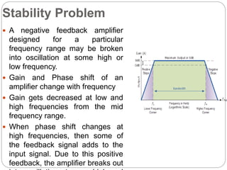
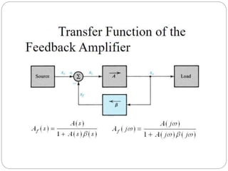
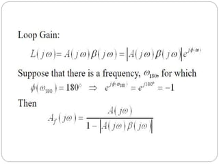
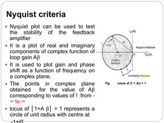
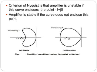
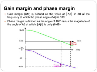
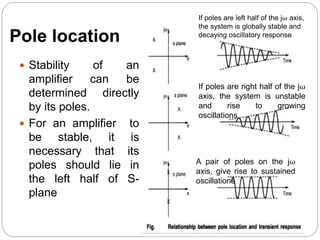
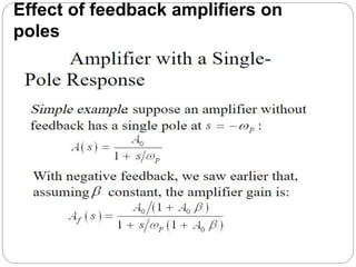
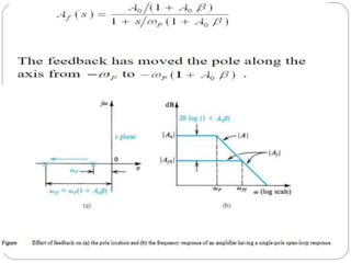
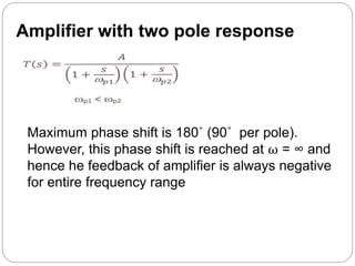
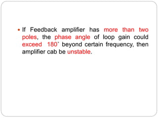
Academic Year 2018-19
EC6401 Electronic Circuits II
Stability problems
Mrs.R.Chitra, AP/ECE,
Ramce Institute f Technology,
Rajapalayam
Stability Problem
 A negative feedback amplifier
designed for a particular
frequency range may be broken
into oscillation at some high or
low frequency.
 Gain and Phase shift of an
amplifier change with frequency
 Gain gets decreased at low and
high frequencies from the mid
frequency range.
 When phase shift changes at
high frequencies, then some of
the feedback signal adds to the
input signal. Due to this positive
feedback, the amplifier breaks out
Contd....
 Stability of feedback amplifier is depend on the
loop gain
 The frequency at which phase angle become
180˚, loop gain A(jω)β(jω) will be real number with
a negative sign.
 Thus at this frequency, the feedback will become
positive, it will behave like an Oscillator.
Nyquist criteria
 Nyquist plot can be used to test
the stability of the feedback
amplifier
 It is a plot of real and imaginary
components of complex function of
loop gain Aβ
 It is used to plot gain and phase
shift as a function of frequency on
a complex plane.
 The points in complex plane
obtained for the value of Aβ
corresponding to values of f from -
∞ to ∞
 locus of │1+A β│ = 1 represents a
circle of unit radius with centre at
 Criterion of Nyquist is that amplifier is unstable if
this curve encloses the point -1+j0
 Amplifier is stable if the curve does not enclose this
point
Gain margin and phase margin
 Gain margin (GM) is defined as the value of │Aβ│ in dB at the
frequency at which the phase angle of Aβ is 180˚
 Phase margin is defined as the angle of 180˚ minus the magnitude of
the angle of Aβ at which │Aβ│ is unity (0 dB)
Pole location
 Stability of an
amplifier can be
determined directly
by its poles.
 For an amplifier to
be stable, it is
necessary that its
poles should lie in
the left half of S-
plane
If poles are left half of the jω axis,
the system is globally stable and
decaying oscillatory response
If poles are right half of the jω
axis, the system is unstable
and rise to growing
oscillations
A pair of poles on the jω
axis, give rise to sustained
oscillations
Effect of feedback amplifiers on
poles
 The pole of amplifier is shift towards left from
imaginary axis and it never enters the right-
half of the s-plane.
 Single pole amplifier introduce a maximum
phase shift of 90˚
 Because of this, a single pole amplifier s
stable for any values of β and hence such an
amplifier is also known as unconditionally
stable amplifier
Amplifier with two pole response
Maximum phase shift is 180˚ (90˚ per pole).
However, this phase shift is reached at ω = ∞ and
hence he feedback of amplifier is always negative
for entire frequency range
 If Feedback amplifier has more than two
poles, the phase angle of loop gain could
exceed 180˚ beyond certain frequency, then
amplifier cab be unstable.
References:
 Sedra and Smith, “Micro Electronic Circuits”;
Sixth Edition, Oxford University Press, 2011.
 Jacob Millman, ‗Microelectronics‘, McGraw Hill,
2nd Edition, Reprinted, 2009.

Stability problems

  • 1.
    Academic Year 2018-19 EC6401Electronic Circuits II Stability problems Mrs.R.Chitra, AP/ECE, Ramce Institute f Technology, Rajapalayam
  • 2.
    Stability Problem  Anegative feedback amplifier designed for a particular frequency range may be broken into oscillation at some high or low frequency.  Gain and Phase shift of an amplifier change with frequency  Gain gets decreased at low and high frequencies from the mid frequency range.  When phase shift changes at high frequencies, then some of the feedback signal adds to the input signal. Due to this positive feedback, the amplifier breaks out
  • 5.
    Contd....  Stability offeedback amplifier is depend on the loop gain  The frequency at which phase angle become 180˚, loop gain A(jω)β(jω) will be real number with a negative sign.  Thus at this frequency, the feedback will become positive, it will behave like an Oscillator.
  • 6.
    Nyquist criteria  Nyquistplot can be used to test the stability of the feedback amplifier  It is a plot of real and imaginary components of complex function of loop gain Aβ  It is used to plot gain and phase shift as a function of frequency on a complex plane.  The points in complex plane obtained for the value of Aβ corresponding to values of f from - ∞ to ∞  locus of │1+A β│ = 1 represents a circle of unit radius with centre at
  • 7.
     Criterion ofNyquist is that amplifier is unstable if this curve encloses the point -1+j0  Amplifier is stable if the curve does not enclose this point
  • 8.
    Gain margin andphase margin  Gain margin (GM) is defined as the value of │Aβ│ in dB at the frequency at which the phase angle of Aβ is 180˚  Phase margin is defined as the angle of 180˚ minus the magnitude of the angle of Aβ at which │Aβ│ is unity (0 dB)
  • 9.
    Pole location  Stabilityof an amplifier can be determined directly by its poles.  For an amplifier to be stable, it is necessary that its poles should lie in the left half of S- plane If poles are left half of the jω axis, the system is globally stable and decaying oscillatory response If poles are right half of the jω axis, the system is unstable and rise to growing oscillations A pair of poles on the jω axis, give rise to sustained oscillations
  • 10.
    Effect of feedbackamplifiers on poles
  • 12.
     The poleof amplifier is shift towards left from imaginary axis and it never enters the right- half of the s-plane.  Single pole amplifier introduce a maximum phase shift of 90˚  Because of this, a single pole amplifier s stable for any values of β and hence such an amplifier is also known as unconditionally stable amplifier
  • 13.
    Amplifier with twopole response Maximum phase shift is 180˚ (90˚ per pole). However, this phase shift is reached at ω = ∞ and hence he feedback of amplifier is always negative for entire frequency range
  • 14.
     If Feedbackamplifier has more than two poles, the phase angle of loop gain could exceed 180˚ beyond certain frequency, then amplifier cab be unstable.
  • 15.
    References:  Sedra andSmith, “Micro Electronic Circuits”; Sixth Edition, Oxford University Press, 2011.  Jacob Millman, ‗Microelectronics‘, McGraw Hill, 2nd Edition, Reprinted, 2009.