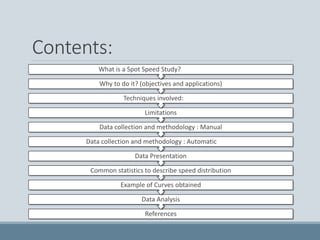
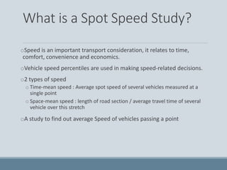
The document is a detailed study on spot speed surveys, including methodology, objectives, limitations, and data analysis techniques used to measure vehicle speeds at specific points on roads. It differentiates between manual and automatic data collection methods, discussing their advantages and disadvantages, followed by common statistics used to describe speed distributions. The study emphasizes the importance of understanding vehicle speeds for traffic management, roadway design, and monitoring trends.

1. Spot Speed
Survey/Study
SUBMITTED BY:
PRATYUSH KUMAR
BP/717/2016
SCHOOL OF PLANNING AND ARCHITECTURE,
DELHI

2. Contents:
References
Data Analysis
Example of Curves obtained
Common statistics to describe speed distribution
Data Presentation
Data collection and methodology : Automatic
Data collection and methodology : Manual
Limitations
Techniques involved:
Why to do it? (objectives and applications)
What is a Spot Speed Study?

3. What is a Spot Speed Study?
oSpeed is an important transport consideration, it relates to time,
comfort, convenience and economics.
oVehicle speed percentiles are used in making speed-related decisions.
o2 types of speed
o Time-mean speed : Average spot speed of several vehicles measured at a
single point
o Space-mean speed : length of road section / average travel time of several
vehicle over this stretch
oA study to find out average Speed of vehicles passing a point

4. Why do it? (Objectives and
Applications)
oTo estimate distribution of speeds in a stream of traffic at a point in a
road or street or highway.
oDetermine speed distribution of a traffic stream at a specific location
oDetermine vehicle speed percentiles
oEstablish roadway design elements like zebra crossings or pedestrian
signal if necessary
oMonitor traffic speed trends by systematic ongoing speed studies

5. Techniques involved:
oTechniques can be majorly classified into two categories:
o Manual
o Automatic
o Road detectors
o Radar based
o Using principles of electronics
oA sample size ranging from 50 to 100 to even 200 can be taken,
depending on the scale and intensity of the study.
oLength to be studied is decided as per following table:
Stream Speed Length
below 15 30
15 -25 60
above 25 90

6. Limitations
oAffected by physical features of roads, like pavement width, curve sight
distance, gradient, pavement unevenness, intersections and road side
developments.
oEnvironmental conditions, enforcement, traffic condition, vehicle,
driver and motive of travel.
oDifficult to spot typical vehicles and so number of observations will be
less
oHuman error
oValid only for the time of test and study.

7. Data collection and
methodology : Manual
Manual:
◦ Spot speeds may be estimated by manually measuring the time it takes a
vehicle to travel between two defined points on the roadway a known
distance apart (short distance), usually less than 90m.
◦ Distance between two points is generally depending upon the average speed
of traffic stream as per the table already shown
◦ Pavement Marking:
◦ In this method, markings of pavement are placed across the road at each end of trap. Observer
start and stops the watch as vehicle passes lines.
◦ Minimum two observers required to collect the data, of which one is standing at the starting
point to start and stop the stop watch and other one is standing at end point to give indication
to stop the watch when vehicle passes the end line.
Stream Speed Length
below 15 30
15 -25 60
above 25 90

8. Data collection and
methodology : Manual
Pavement marking continued:
◦ Advantage: after the initial installation no set-up time is required, markings
are easily renewed.
◦ Disadvantage:
◦ substantial error can be introduced, and magnitude of error may change for substitute studies.
◦ This method is only applicable for low traffic conditions.
CAR
Begin
Timing
End
Timing
50-90 meters

9. Enoscopic or mirror box
◦ Enoscope consists of a simple open housing containing a
mirror mounted on a tripod at the side of the road in such
a way that an observer’s line of sight turned through 90
degrees.
◦ Observer stands at one end and on other end enoscope is
placed and time taken to cross the section is measured
◦ Advantage: simple and eliminates errors due to parallax
◦ Disadvantage: Takes considerable time per vehicle, under
heavy traffic it is difficult to relate ostentatious to proper
vehicle.
Data collection and
methodology : Manual

10. Data collection and
methodology : Automatic
Pneumatic tube method
◦ Tube laid beneath track
◦ Pressure contact strips, either pneumatic or
electric used to indicate time of entering and
laving base length (usually 2 to 5 meters)
◦ Stopwatch starts by electric impulse generated
when vehicle runs over first tube, stops when
vehicle passes second tube.
◦ Advantage:
◦ Human error reduced, parallax error completely removed,
best method in short distance, relevant data, can give
continuous stream too.
◦ Disadvantage:
◦ Pressure contact tubes are easily sensed by drivers which
may affect their behavior.

11. Data collection and
methodology : Automatic
Doppler principle meter (radar)
◦ Measures speed directly by measuring
difference in frequency between emitted
and received wave.
◦ It uses the doppler effect
◦ Limitations:
◦ Possibility of recording wrong input from another
vehicle rebounding the waves.
◦ Accurate measurement from radar mater obtained
only if radar wave is reflected directly along axis of
movement.

12. Data collection and
methodology : Automatic
Electronic Principle Detectors
◦ A camera records the distance moved by a
vehicle in a selected short time.
◦ Exposure of photograph in constant time
interval and distance travelled by vehicle
measured by projecting the films during
exposure interval.
◦ Video recorders may also be used, they give
more accurate results.
◦ Advantage:
◦ Gives permanent record with 100% sample obtained.
◦ Used where evidence is needed
◦ Disadvantage:
◦ Is very expensive

13. Data Presentation
▪Frequency Distribution Table
▪ Arrange speed data points in ascending order
▪ Select a class interval and arrange it in this range.
▪Frequency distribution Curve
▪ % frequency of observations within the group is plotted versus the middle
▪ modal speed and pace of traffic flow can be determined
▪ Generally follows a normal curve
▪Cumulative Frequency distribution Curve
▪ For each speed group, the % cumulative frequency of observations is plotted
versus the higher limit of the speed group.
▪ Results in a very useful plot of speed versus the percent of vehicles traveling
at or below the designated speed
▪ plots the upper limit of the speed group (NOT the middle speed)

14. Common statistics to describe
speed distribution
oMeasures of central tendency
o Average/Mean speed:
o Time mean : If data collected over a period of time.
o Space mean : If data collected over a stretch of road lenth
o Median speed : Equally divides the distribution into two halves.
o Pace: The 10km/h gap in which most % of drivers are observed
o Modal Speed : Single value of speed that is most likely to occur.
oMeasures of Dispersion
o Standard Deviation : To measure how far data spreads around mean value.
o %vehicle within the pace: smaller the percentage, greater the degree of
dispersion
o Percentile speeds:
o 85th and 15th percentile give general description of high and low speeds observed by most
drivers.
o Found from the CF distribution curve
o Standard deviation of the distribution is found out by this : σest = (v85 – v15 )/2

15. Example of Curves obtained
0%
2%
4%
6%
8%
10%
12%
14%
16%
18%
20%
0%
20%
40%
60%
80%
100%
120%
21-25 26-30 31-35 36-40 41-45 46-50 51-55 56-60 61-65 66-70 71-75 76-80
%
SPEED (KMPH)
%cf fi %

16. Data Analysis
oStandard error of the mean:
o The means of different sample taken from the same population are
distributed normally about the true mean of population with a standard
deviation, is known as standard error.
o Given as: Se = σs /√n
oConfidence Interval:
o Confidence intervals express the range within which a result for the whole
population would occur for a particular proportion of times an experiment
or test was repeated among a sample of the population
o Calculated as: μ = vt ± (Z*Se); μ= confidence interval, vt = mean speed, Z= Z
statistic for given confidence, Se = Standard error; Z*Se = Margin of error.
oSample size: Generally sample of 50-200 vehicles is taken, but the
number can be found out using the formula
o n=(Z*σs / Se)2

17. References
NPTEL (National Programme on Technology Enhanced Learning) Module 2: Traffic Measurement
Procedures, Lecture 6: Measurement over a short Section
Spot Speed and Speed Delay Time Survey, project, Dept of Civil Engineering, Gokaraju Rangaraju
Institute of Engineering and Technology, Hyderabad
Bangladesh University of Engineering and Technology, Spot Speed Survey Report
Homburger, W. S., J. W. Hall, R. C. Loutzenheiser, and W. R. Reilly. 1996. Spot Speed Studies. In
Fundamentals of Traffic Engineering. Berkeley: Institute of Transportation Studies,University of
California, Berkeley, pp. 6.1–6.9.
Robertson, H. D. 1994. Spot Speed Studies. In Manual of Transportation Engineering Studies, ed. H. D.
Robertson, J. E. Hummer, D. C. Nelson. Englewood Cliffs, N.J.: Prentice Hall,Inc
Currin, T. R. 2001. Spot Speed Study. In Introduction to Traffic Engineering: A Manual for Data
Collection and Analysis, ed. B. Stenquist. Stamford, Conn.: Wadsworth Group,
Dr. Tom V. Mathew 2014. Chapter6 Measurement over a Short Section. Transportation Systems
Engineering. IIT Bombay.
Dr. Tom V. Mathew and K.V. Krishna Rao 2007. Traffic Data Collection. Introduction to Transport
Engineering. NPTEL.
Dr. Bhargab Maitra. Lecture 5 Traffic Stream Characteristics. Introduction to Transport Engineering.
Department of Civil Engineering, IIT Kharagpur.

18. Thank You for your patience!