B tech traffic engineering study material

1. TRANSPORTATION ENGINEERING
Course code: CE 2302
Program: B. Tech.
Semester: Fourth (Credit: 3)
Course instructor
Dr. Aditya Kumar Das
Assistant Professor
Department of Civil Engineering
National Institute of Technology Rourkela
Traffic Engineering Studies
 The availability of highway transportation has provided several advantages that
contribute to a high standard of living. However several problems related to the
highway mode of transportation exist. These problems include highway-related
crashes, parking difficulties, congestion, and delay.
 To reduce the negative impact of highways, it is necessary to adequately collect
information that describes the extent of the problems and identifies their
locations.
 Such information is usually collected by organizing and conducting traffic surveys
and studies.
 This topic introduces the reader to the different traffic engineering studies that are
conducted to collect traffic data.
 Brief descriptions of the methods of collecting and analyzing the data are also
included.
Traffic Studies
Traffic studies are grouped into three main
categories:
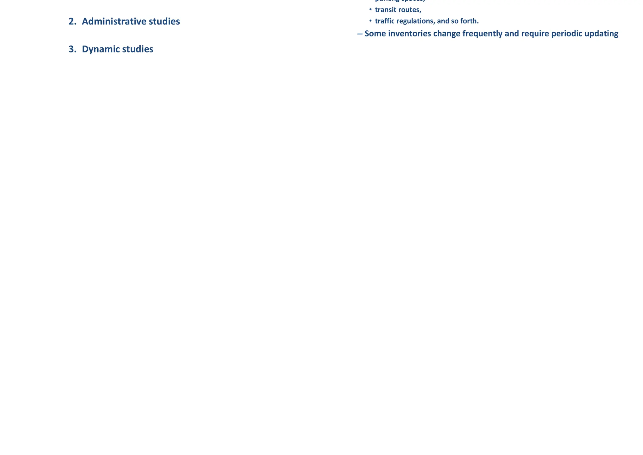
1. Inventories
2. Administrative studies
3. Dynamic studies
Traffic Studies
• Inventories :
– Provide a list or graphic display of existing information such as
• street widths,
• parking spaces,
• transit routes,
• traffic regulations, and so forth.
– Some inventories change frequently and require periodic updating

2. Traffic Studies
• Administrative studies :
– use existing engineering records, available in
government agencies and departments.
– include the results of surveys, which may involve:
• field measurements and/or
• aerial photography.
– above Information is recorded in files or in automated data processing
(ADP) systems
Traffic Studies
• Dynamic Traffic studies :
– involve the collection of data under operational
conditions and include studies of:
• speed,
• traffic volume,
• travel time and delay,
• parking, and
• crashes
– They are described in detail here.
Spot speed studies
– conducted to estimate the distribution of speeds of vehicles in a stream of traffic at a
particular location on a highway.
– The speed of a vehicle is defined as the rate of movement of the vehicle; it is usually
expressed in miles per hour (mi/h) or kilometers per hour (km/h)
– carried out by recording the speeds of a sample of vehicles at a specified location.
– Speed characteristics identified by such a study will be valid only for the traffic and
environmental conditions that exist at the time of the study.
Spot speed studies
Spot Speed: Spot speed is the instantaneous speed of a vehicle at a particular section or
location of the road.
Average Speed
As its name, the average speed is the average of all spot speeds of various vehicles
passing through a given point or section.
Running Speed
Running speed is the average speed maintained by a vehicle over a particular stretch
of road.
Travel or Journey speed
Journey speed the effective speed of travel of all vehicles along the route between two
terminals.

3. Spot speed studies
Types of Spot Speed
1.Space Mean Speed
Space mean speed is the average speed of vehicles in a certain road length at
any specified time period. It is very useful for determining vehicle flow
characteristics.
𝑉 =
3.6𝑑𝑛
∑ 𝑡
d is length of road m, n is no. of individual vehicle observations, t1 is observed
travel time (sec) for ith vehicle to travel distance d m.
2.Time Mean Speed
Time mean speed is the average speed of vehicles passing a point over some
specified time period.
𝑉 =
∑ 𝑉
𝑛
Vi is observed instantaneous speed of ith vehicle, kmph, n is no. of vehicle
observed.
Spot speed studies
– Minimum number of sample size is given by:
– where
N = minimum sample size
Z = number of standard deviations corresponding to
the required confidence level =1.96 for 95 percent
confidence level
s = standard deviation (mi/h)
d = limit of acceptable error in the average speed
estimate (mi/h)
Presentation and Analysis of Spot Speed Data Presentation and Analysis of Spot Speed Data
98% speed= design speed
85% speed= maximum limiting speed
15% speed= lower speed limit
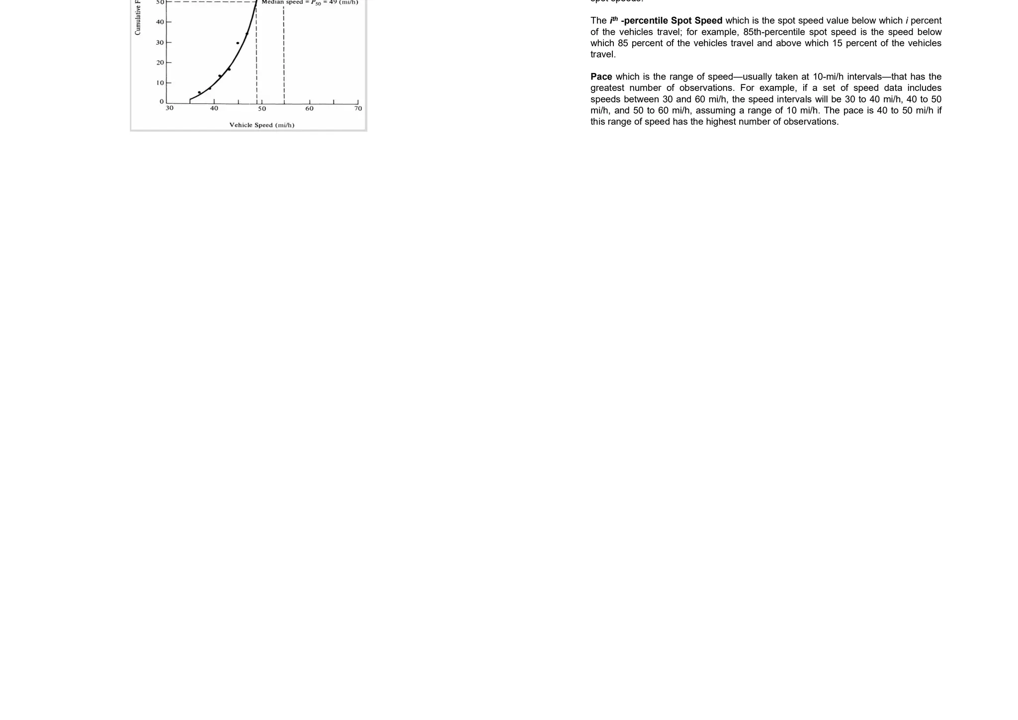
Median Speed which is the speed at the middle value in a series of spot speeds that
are arranged in ascending order. 50 percent of the speed values will be greater than
the median; 50 percent will be less than the median
Modal Speed which is the speed value that occurs most frequently in a sample of
spot speeds.
The ith -percentile Spot Speed which is the spot speed value below which i percent
of the vehicles travel; for example, 85th-percentile spot speed is the speed below
which 85 percent of the vehicles travel and above which 15 percent of the vehicles
travel.
Pace which is the range of speed—usually taken at 10-mi/h intervals—that has the
greatest number of observations. For example, if a set of speed data includes
speeds between 30 and 60 mi/h, the speed intervals will be 30 to 40 mi/h, 40 to 50
mi/h, and 50 to 60 mi/h, assuming a range of 10 mi/h. The pace is 40 to 50 mi/h if
this range of speed has the highest number of observations.

4. NP1
Using the spot speed data given in the following table,
collected from a freeway site operating under free-flow
conditions:
(i) Plot the frequency and cumulative frequency curves for
these data;
(ii) Obtain median speed, modal speed, pace, and percent
vehicles in pace from these plots;
(iii) Compute the mean and standard deviation of the speed
distribution;
(iv) The confidence bounds on the estimate of the true mean
speed of the underlying distribution with 95%
confidence? With 99.7% confidence; and
(v) Based on these results, compute the sample size needed
to achieve a tolerance of±1.5 kmph with 95%
confidence.
NP1…..
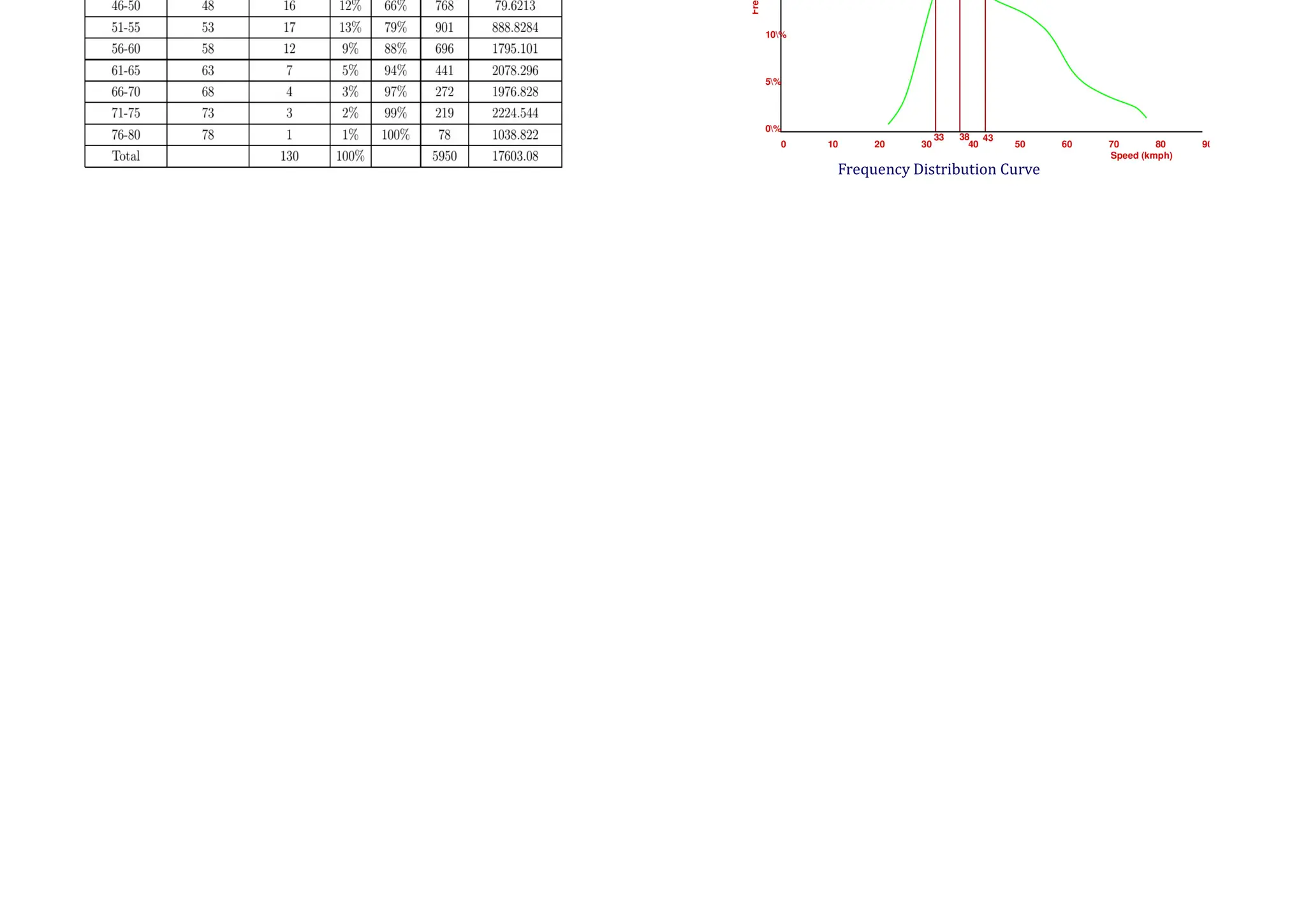
Solution Solution From the curves, Median speed, v50 = 43 kmph;
Modal speed, = 38 kmph; the Pace = 33 - 43 kmph;
Percent vehicles in pace = 54-20= 34%; and
85th Percentile speed = 58 kmph.
Frequency Distribution Curve

5. Solution
Cumulative Frequency Distribution Curve
Solution
Mean is calculated by using
Standard Deviation of the Speed
Solution
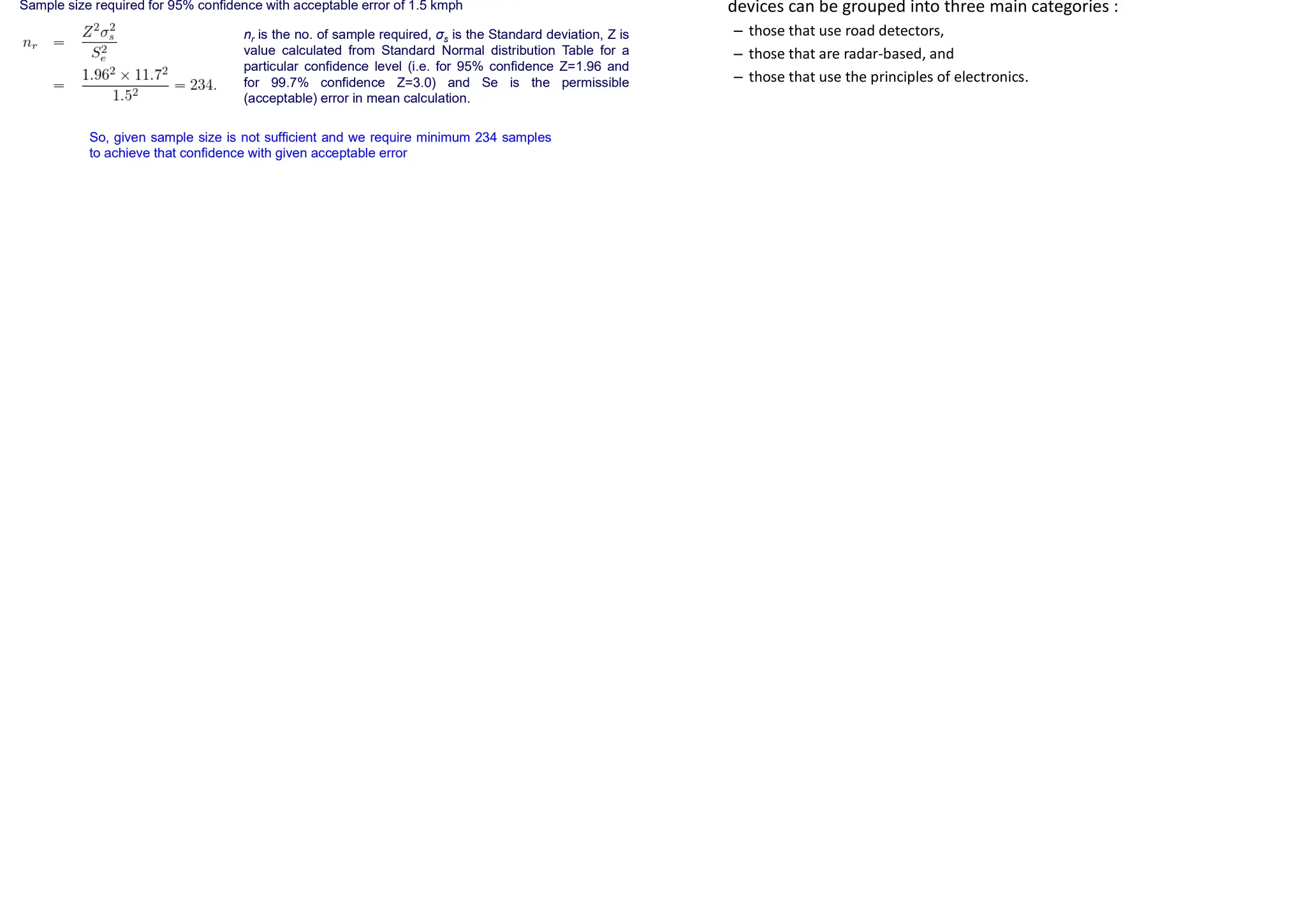
Sample size required for 95% confidence with acceptable error of 1.5 kmph
So, given sample size is not sufficient and we require minimum 234 samples
to achieve that confidence with given acceptable error
nr is the no. of sample required, σs is the Standard deviation, Z is
value calculated from Standard Normal distribution Table for a
particular confidence level (i.e. for 95% confidence Z=1.96 and
for 99.7% confidence Z=3.0) and Se is the permissible
(acceptable) error in mean calculation.
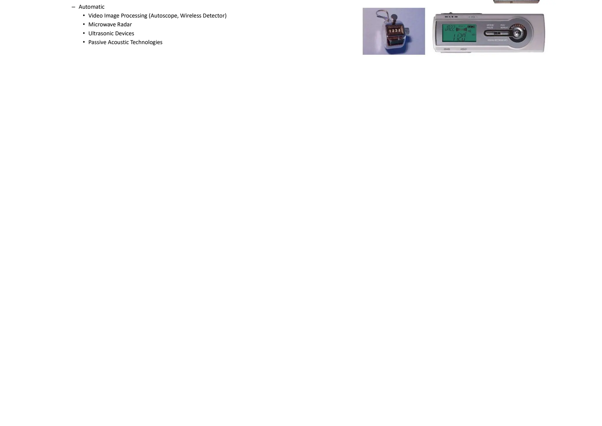
Methods for Conducting Spot Speed Studies
• Several automatic devices that can be used to obtain the
instantaneous speeds of
vehicles at a location on a highway are now available on the market.
These automatic
devices can be grouped into three main categories :
– those that use road detectors,
– those that are radar-based, and
– those that use the principles of electronics.

6. Methods for Conducting Spot Speed Studies
Pavement markings
Vertical reference
point
Start time
Vertical reference
point
End time
Methods for Conducting Spot Speed Studies
Enoscope or Mirror box
• Enoscope consists of a simple open housing
containing a mirror mounted on a tripod at the
side of the road in such a way that an observer’s
line of sight turned through 90o.
• The observer stands at one end of section and on
the other end enoscope is placed and measure
the time taken by the vehicle to cross the section
Methods for Conducting Spot Speed Studies
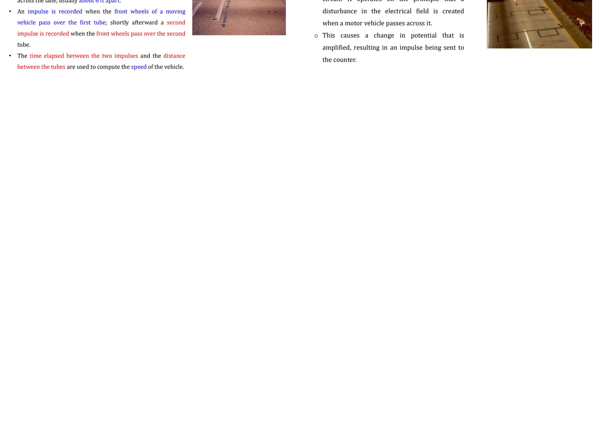
• Pneumatic road tubes are laid across the lane in which data
are to be collected.
• When a moving vehicle passes over the tube, an air impulse is
transmitted through the tube to the counter.
• When used for speed measurements, two tubes are placed
across the lane, usually about 6 ft apart.
• An impulse is recorded when the front wheels of a moving
vehicle pass over the first tube; shortly afterward a second
impulse is recorded when the front wheels pass over the second
tube.
• The time elapsed between the two impulses and the distance
between the tubes are used to compute the speed of the vehicle.
Methods for Conducting Spot Speed Studies
o An inductive loop is a rectangular wire loop
buried under the roadway surface.
o It usually serves as the detector of a resonant
circuit. It operates on the principle that a
disturbance in the electrical field is created
when a motor vehicle passes across it.
o This causes a change in potential that is
amplified, resulting in an impulse being sent to
the counter.

7. Methods for Conducting Spot Speed Studies
• Radar-based traffic sensors work on the principle
that when a signal is transmitted onto a moving
vehicle, the change in frequency between the
transmitted signal and the reflected signal is
proportional to the speed of the moving vehicle.
• The difference between the frequency of the
transmitted signal and that of the reflected signal
is measured by the equipment and then
converted to speed in kmph.
Methods for Conducting Spot Speed Studies
• In this method, the presence of vehicles is detected
through electronic means, and information on these
vehicles is obtained, from which traffic characteristics,
such as speed, volume, queues, and headways are
computed.
• The great advantage of this method over the use of road
detectors is that it is not necessary to physically install
loops or any other type of detector on the road.
• A technology using electronics is video image processing,
sometimes referred to as a machine-vision system.
• This system consists of an electronic camera overlooking
a large section of the roadway and a microprocessor.
• The electronic camera receives the images from the road;
the microprocessor determines the vehicle’s presence or
passage.
• This information is then used to determine the traffic
characteristics in real time. One such system is the
autoscope CCTV?
Volume Studies
• Traffic volume studies are conducted to collect data on the number of vehicles and/or
pedestrians that pass a point on a highway facility during a specified time period.
• Traffic volume is expressed as vehicle/h or vehicle/day
• This time period varies from as little as 15 minutes to as much as a year depending on the
anticipated use of the data.
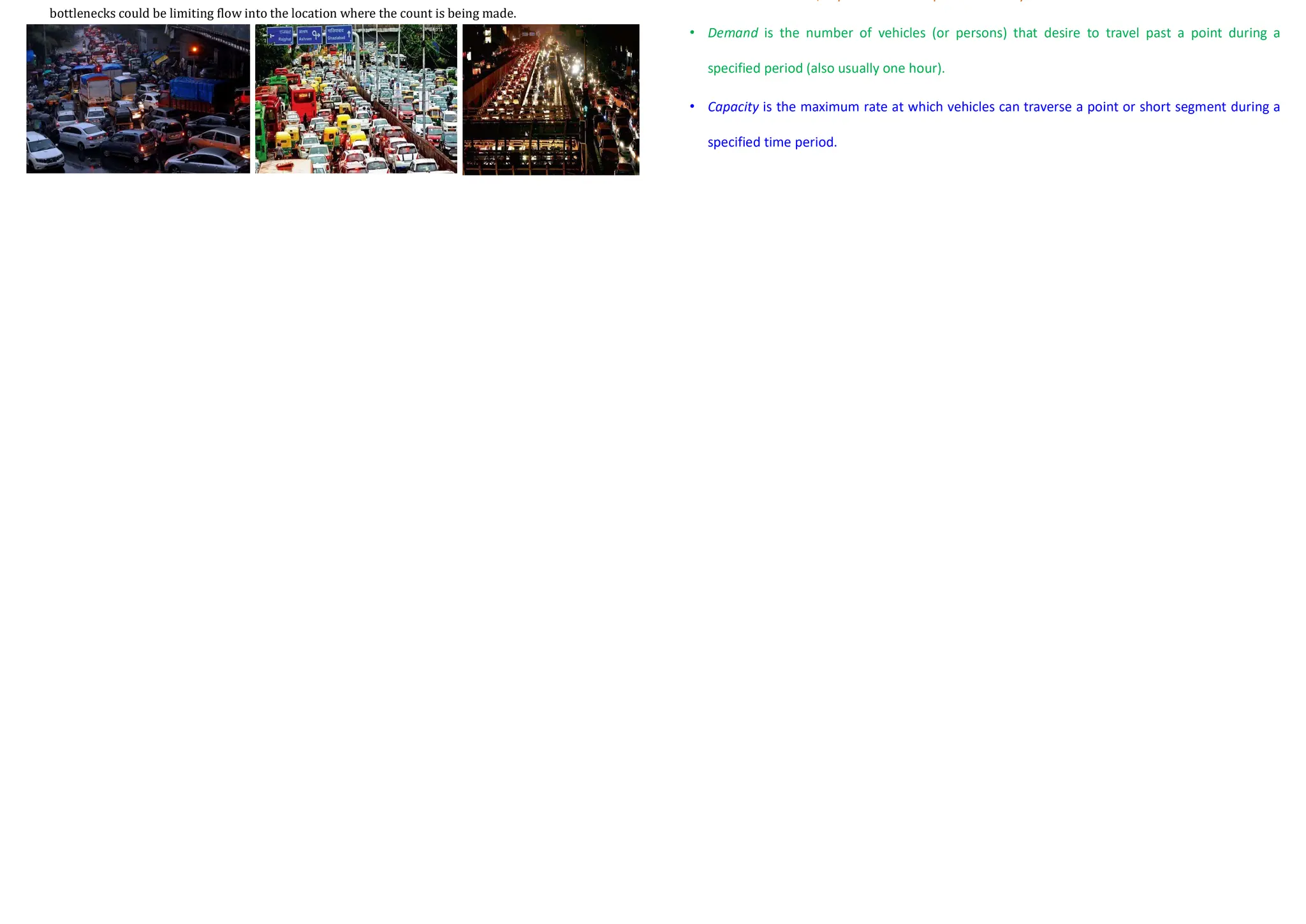
• When selecting locations for volume counts, it is important to note whether upstream
bottlenecks could be limiting flow into the location where the count is being made.
Volume, Flow Rate, Demand, Capacity
• Volume is the number of vehicles (or persons) passing a point during a specified time period,
which is usually one hour, but need not be.
• Rate of flow is the rate at which vehicles (or persons) pass a point during a specified time period
less than one hour, expressed as an equivalent hourly rate.
• Demand is the number of vehicles (or persons) that desire to travel past a point during a
specified period (also usually one hour).
• Capacity is the maximum rate at which vehicles can traverse a point or short segment during a
specified time period.

8. Passenger Car Unit (PCU)
• PCU is a metric used in Transportation Engineering, to assess traffic-flow rate on a
highway.
• PCU is a measure of the impact that a mode of transport has on traffic variables
(such as headway, speed, density) compared to a single standard passenger car. This
is also known as passenger car equivalent.
• Highway capacity is measured in PCU/hour daily.
• For example, typical values of PCU (or PCE) are:
– Car 1.0;
– Motorcycle 0.5 ;
– Bicycle 0.2;
– LCV 2.2 ;
– Bus, Truck 3.5;
– 3-wheeler 0.8
Volume Studies
• Traffic volume studies are usually conducted when certain volume characteristics are needed as
follows:
– DAILY VOLUMES
• Annual Average Daily Traffic (AADT)
• Average Daily Traffic (ADT)
– HOURLY VOLUMES
• Peak hour volume (PHV)
• Directional Design Hourly Volume(DDHV)
– SUB HOURLY VOLUMES
• Peak Hour Factor
– Vehicle Classification
– Vehicle Kms of Travel (VKT) [Vehicle Miles of Travel , (VMT)]
Annual Average Daily Traffic (AADT)
• Average of 24-hour counts collected every day of the year
• Considers seasonal variation of daily traffic within a year
• Used in several traffic and transportation analyses for:
– Estimation of highway user revenues
– Computation of crash rates in terms of number of crashes per 100 million vehicle miles
– Establishment of traffic volume trends
– Evaluation of the economic feasibility of highway projects
– Development of freeway and major arterial street systems
– Development of improvement and maintenance programs
Average Daily Traffic (ADT)
• Average of 24-hour counts collected over a number of days greater than one but less than a year
• Considers day to day variation of traffic (say, within a week)
• Used in several traffic and transportation analyses for:
– Planning of highway activities
– Measurement of current demand
– Evaluation of existing traffic flow

9. Peak Hour Volume (PHV)
• Maximum number of vehicles that pass a point on a highway during a period of 60 consecutive
minutes
• Reflects hourly variation of traffic within a day
• Used for:
– Functional classification of highways
– Design of the geometric characteristics of a highway, for example, number of lanes,
intersection signalization, or channelization
– Capacity analysis
– Development of programs related to traffic operations, for example, one-way street systems
or traffic routing
– Development of parking regulations
Types of Volume Counts
• Cordon Counts
• Screen Line Counts
• Intersection Counts
• Pedestrian Volume Counts
• Periodic Volume Counts
– Continuous
– Control
– Coverage
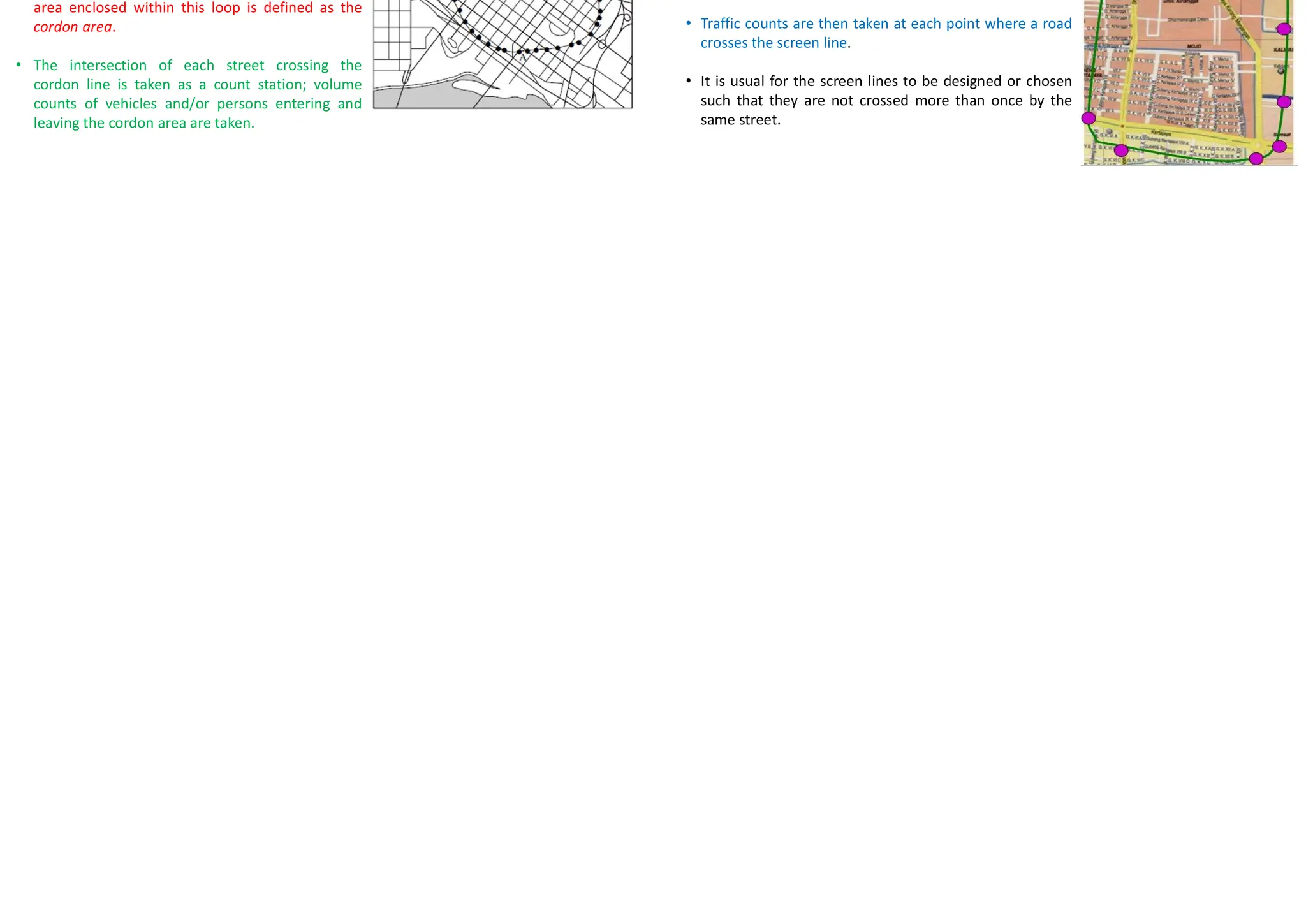
Cordon Counts
• When information is required on vehicle
accumulation within an area such as the central
business district (CBD) of a city, particularly during
a specific time, a cordon count is undertaken.
• The area for which the data are required is
cordoned off by an imaginary closed loop; the
area enclosed within this loop is defined as the
cordon area.
• The intersection of each street crossing the
cordon line is taken as a count station; volume
counts of vehicles and/or persons entering and
leaving the cordon area are taken.
Screen Line Counts
• In screen line counts, the study area is divided into large
sections by running imaginary lines, known as screen
lines, across it.
• In some cases, natural and manmade barriers, such as
rivers or railway tracks, are used as screen lines.
• Traffic counts are then taken at each point where a road
crosses the screen line.
• It is usual for the screen lines to be designed or chosen
such that they are not crossed more than once by the
same street.

10. Cordon and Screen Line Counts Intersection Counts
• Intersection counts are taken to determine
vehicle classifications, through movements, and
turning movements at intersections.
• These data are used mainly in determining phase
lengths and cycle times for signalized
intersections, in the design of channelization at
intersections, and in the general design of
improvements to intersections.
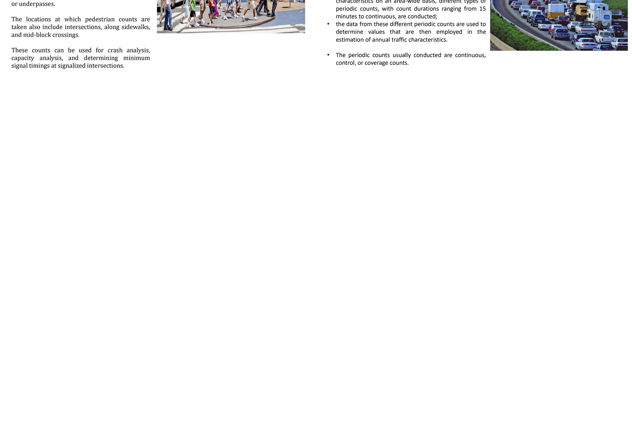
Pedestrian Volume Counts
Volume counts of pedestrians are made at
locations such as subway stations, midblocks, and
crosswalks.
The counts are usually taken at these locations
when the evaluation of existing or proposed
pedestrian facilities is to be undertaken.
Such facilities may include pedestrian overpasses
or underpasses.
The locations at which pedestrian counts are
taken also include intersections, along sidewalks,
and mid-block crossings.
These counts can be used for crash analysis,
capacity analysis, and determining minimum
signal timings at signalized intersections.
Periodic Volume Counts :
Continuous, Control, Coverage
• In order to obtain certain traffic volume data, such as
AADT, it is necessary to obtain data continuously.
• However, it is not feasible to collect continuous data on
all roads because of the cost involved.
• To make reasonable estimates of annual traffic volume
characteristics on an area-wide basis, different types of
periodic counts, with count durations ranging from 15
minutes to continuous, are conducted;
• the data from these different periodic counts are used to
determine values that are then employed in the
estimation of annual traffic characteristics.
• The periodic counts usually conducted are continuous,
control, or coverage counts.

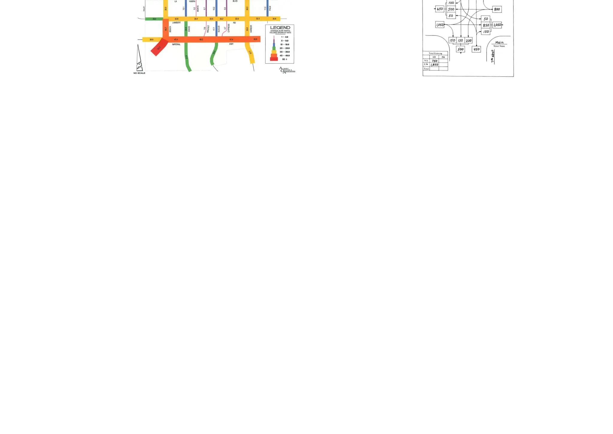
11. Presentation & Analysis of Volume Counts
• Traffic Flow Maps
• Intersection Summary Sheets
• Time Based Distribution Charts
• Summary Tables
Traffic Flow Maps
Intersection Summary Sheets

12. Time Based Distribution Charts
Summary Tables
Methods for Conducting Volume Counts
• Intrusive (Automatic)
– Pneumatic Road Tubes
– Piezoelectric Sensors
– Inductive Loops
• Non-Intrusive
– Manual
– Automatic
• Video Image Processing (Autoscope, Wireless Detector)
• Microwave Radar
• Ultrasonic Devices
• Passive Acoustic Technologies
Methods for Conducting Volume Counts

13. Methods for Conducting Volume Counts Methods for Conducting Volume Counts
Methods for Conducting Volume Counts Flow:
• Flow or volume are the two ways of counting the number of vehicles on a road.
• Number of vehicles that pass a point on a highway during a specific time interval.
• Mathematically the flow ‘q’ is expressed in vehicles/hour is given by
t
n
q
t

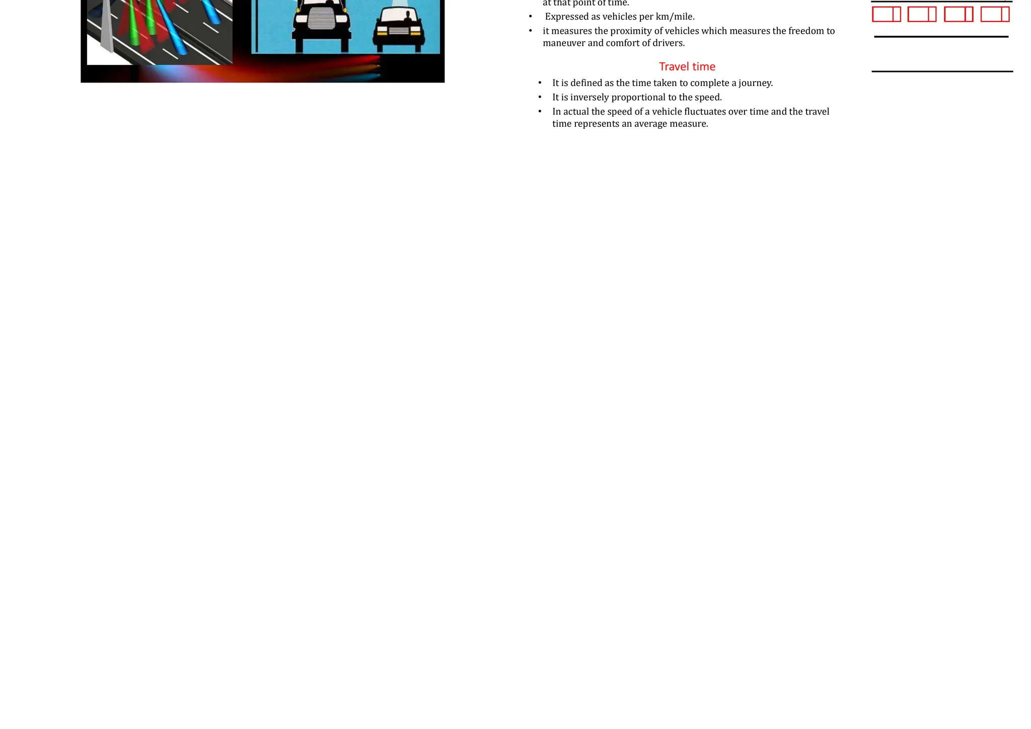
Density:
• It is defined as the number of vehicles occupying a given length of highway.
• x is length of the road, 𝑛 is the number of vehicles in one lane of the road
at that point of time.
• Expressed as vehicles per km/mile.
• it measures the proximity of vehicles which measures the freedom to
maneuver and comfort of drivers.
Travel time
• It is defined as the time taken to complete a journey.
• It is inversely proportional to the speed.
• In actual the speed of a vehicle fluctuates over time and the travel
time represents an average measure.
x
n
k
x


14. Fundamental Relations of Traffic Flow
The relationship between the fundamental variables of traffic flow, namely speed, volume, and density
is called the fundamental relations of traffic flow. This can be derived by a simple concept. Let there be
a road with length v km, and assume all the vehicles are moving with v km/hr.(Fig).
Let the number of vehicles counted by an observer at A
for one hour be n1. By definition, the number of vehicles
counted in one hour is flow(q). Therefore n1 = q
Similarly, by definition, density is the number of vehicles in unit
distance. Therefore number of vehicles n2 in a road stretch of
distance v1 will be density × distance. Therefore, n2 = k * v
Since all the vehicles have speed v, the number of vehicles
counted in 1 hour and the number of vehicles in the stretch of
distance v will also be same.(ie n1 = n2). Therefore, q = k*v
This is the fundamental equation of
traffic flow. Please note that, v in the
above equation refers to the space
mean speed will also be same.
Fundamental Relations of Traffic Flow
Fundamental diagrams  The relation between flow and density, density and speed, speed and
flow, can be represented with the help of some curves
Flow-density curve The flow and density varies with time and location.
• When the density is zero, flow will also be zero, since
there is no vehicles on the road.
• When the number of vehicles gradually increases the
density as well as flow increases.
• When more and more vehicles are added, it reaches a
situation where vehicles can’t move. This is referred to as
the jam density or the maximum density. At jam density,
flow will be zero because the vehicles are not moving.
• There will be some density between zero density and jam
density, when the flow is maximum. The relationship is
normally represented by a parabolic curve as shown in
figure.
Fundamental Relations of Traffic Flow
Fundamental diagrams  The relation between flow and density, density and speed, speed and
flow, can be represented with the help of some curves
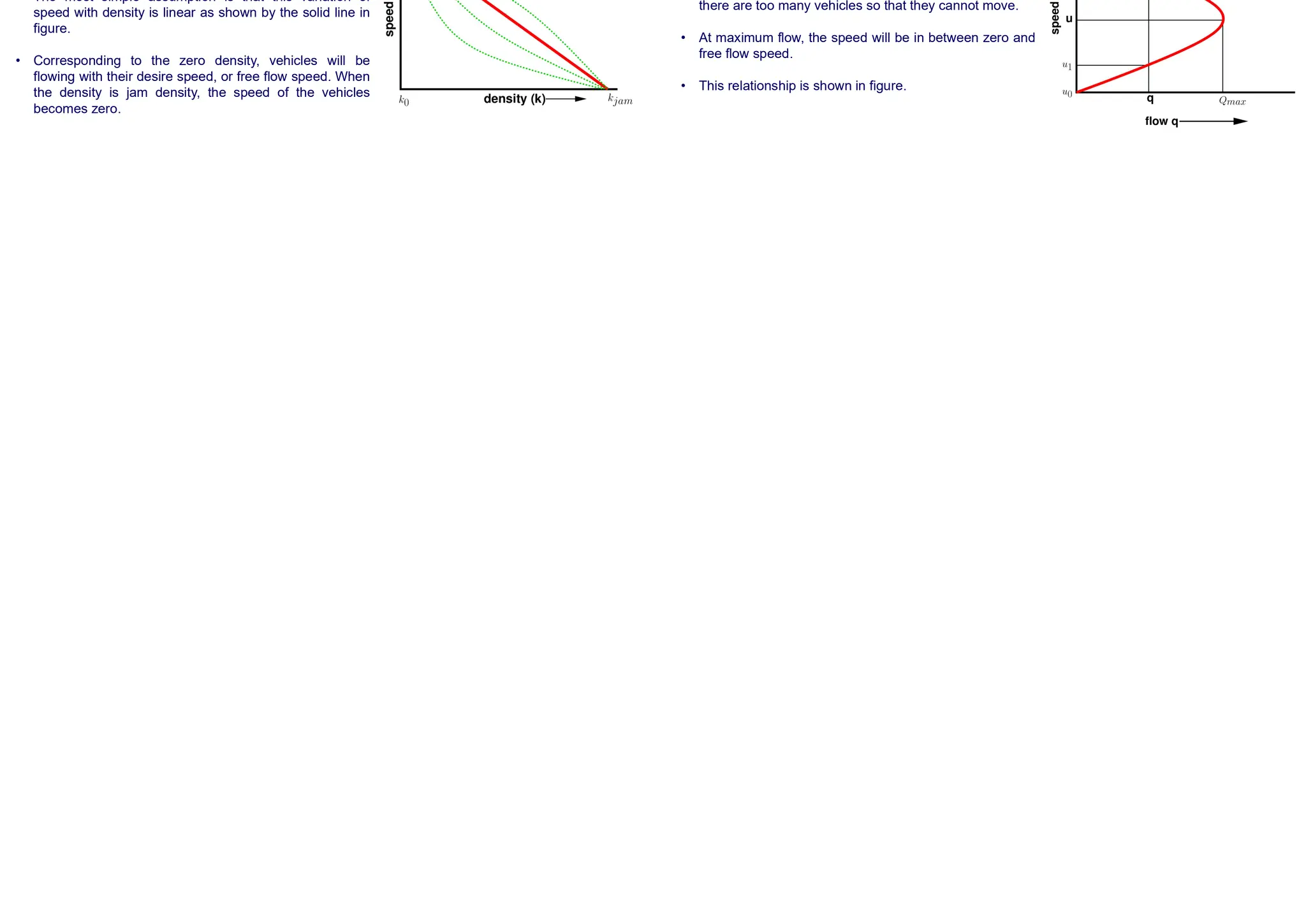
Speed-density diagram The flow and density varies with time and location.
• Similar to the flow-density relationship, speed will be
maximum, referred to as the free flow speed, and when
the density is maximum, the speed will be zero.
• The most simple assumption is that this variation of
speed with density is linear as shown by the solid line in
figure.
• Corresponding to the zero density, vehicles will be
flowing with their desire speed, or free flow speed. When
the density is jam density, the speed of the vehicles
becomes zero.
Fundamental Relations of Traffic Flow
Fundamental diagrams  The relation between flow and density, density and speed, speed and
flow, can be represented with the help of some curves
Speed flow relation The flow and density varies with time and location.
• The relationship between the speed and flow can be
postulated as follows.
• The flow is zero either because there is no vehicles or
there are too many vehicles so that they cannot move.
• At maximum flow, the speed will be in between zero and
free flow speed.
• This relationship is shown in figure.

15. Fundamental Relations of Traffic Flow
Fundamental diagrams  The relation between flow and density, density and speed, speed and
flow, can be represented with the help of some curves
Speed flow relation The flow and density varies with time and location.
• The diagrams shown in the relationship
between speed-flow, speed-density, and
flow-density are called the fundamental
diagrams of traffic flow.
• These are as shown in figure.
• One could observe the inter-relationship of
these diagrams.
PARKING
Parking Studies
Parking accumulation
 It is defined as the number of vehicles parked at a given instant of time. Normally
this is expressed by accumulation curve.
 Accumulation curve is the graph obtained by plotting the number of bays occupied
with respect to time
Parking volume
 Parking volume is the total number of vehicles parked at a given duration of time.
 This does not account for repetition of vehicles
Parking load
 Parking load gives the area under the accumulation curve.
 It can also be obtained by simply multiplying the number of vehicles occupying the
parking area at each time interval with the time interval.
 It is expressed as vehicle hours.
Parking Statistics

16. • It is the ratio of total vehicle hours to the number of vehicles parked
Average parking duration
Cont…
Parking turnover
 It is the ratio of number of vehicles parked in a duration to the number of
parking bays available.
 This can be expressed as number of vehicles per bay per time duration.
Parking index
 Parking index is also called occupancy or efficiency.
 It is defined as the ratio of number of bays occupied in a time duration to
the total space available
Fixed period sampling
 This is almost similar to in-out survey. All vehicles are counted at the beginning of
the survey.
 Then after a fixed time interval that may vary between 15 minutes to i hour, the
count is again taken.
 Here there are chances of missing the number of vehicles that were parked for a
short duration.
Parking surveys are conducted to collect the parking statistics.
In-out survey
 In this survey, the occupancy count in the selected parking lot is taken at the
beginning.
 Then the number of vehicles that enter and leaving the parking lot for a particular
time interval is counted.
 The final occupancy in the parking lot is also taken .
 For this survey only one person may be enough.
 But in this parking duration and turn over is not obtained. Hence parking fare cant
be estimated from this survey.
Parking Surveys
Cont…
License plate method of survey
 This results in the most accurate and realistic data.
 In this case of survey, every parking stall is monitored at a continuous interval of
15 minutes or so and the license plate number is noted down.
 This will give the data regarding the duration for which a particular vehicle was
using the parking bay.
 This will help in calculating the fare because fare is estimated based on the
duration for which the vehicle was parked.
 If the time interval is shorter, then there are less chances of missing short-term
parkers.
 But this method is very labor intensive
Accidents
 Careless maneuvering of parking and un-parking leads to accidents which are
referred to as parking accidents.
 Common type of parking accidents occur while driving out a car from the parking
area, careless opening of the doors of parked cars, and while bringing in the
vehicle to the parking lot for parking.
Congestion
 Parking takes considerable street space leading to the lowering of the road
capacity.
 Hence, speed will be reduced, journey time and delay will also subsequently
increase.
 The operational cost of the vehicle increases leading to great economical loss to
the community
Ill Effects Of Parking

17. Obstruction to fire fighting operations
 Parked vehicles may obstruct the movement of fire fighting vehicles.
 Sometimes they block access to hydrants and access to buildings.
Environmental pollution
 They also cause pollution to the environment because stopping and starting of
vehicles while parking and un-parking results in noise and fumes.
 They also affect the aesthetic beauty of the buildings because cars parked at every
available space creates a feeling that building rises from a plinth of cars.
Cont..
 There are some minimum parking requirements for different types of building
 For residential plot area less than 300 sq.m require only community parking space.
For residential plot area from 500 to 1000 sq.m, minimum one-fourth of the open
area should be reserved for parking
 Offices may require at least one space for every 70 sq.m as parking area
 One parking space is enough for 10 seats in a restaurant
 Theatres and cinema halls need to keep only 1 parking space for 20 seats.
 Thus, the parking requirements are different for different land use zones.
Parking Requirements
On street parking means the vehicles are parked on the sides of the street itself..
Parallel parking
 The vehicles are parked along the length of the road. Here there is no backward
movement involved while parking or un-parking the vehicle. Hence, it is the most
safest parking from the accident perspective.
 It consumes the maximum curb length and therefore only a minimum number of
vehicles can be parked for a given kerb length.
 This method of parking produces least obstruction to the on-going traffic on the
road since least road width is used.
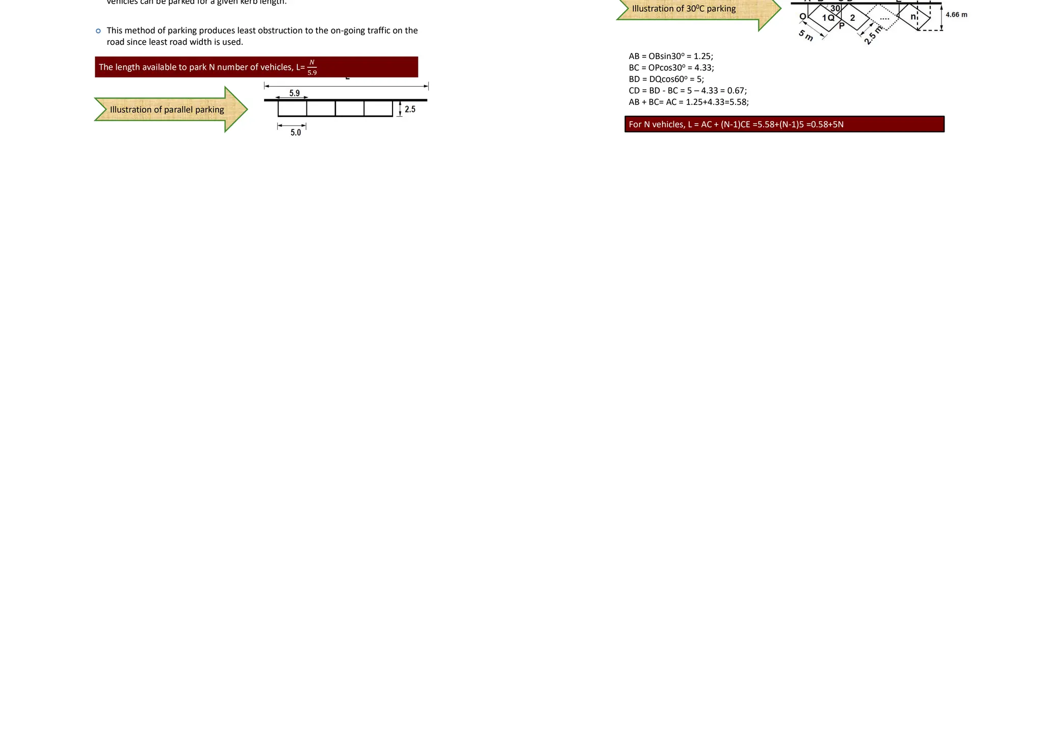
Illustration of parallel parking
On Street Parking
The length available to park N number of vehicles, L= .
Cont..
30oC parking
 In thirty degree parking, the vehicles are parked at 30 with respect to the road
alignment.
 More vehicles can be parked compared to parallel parking.
 Delay caused to the traffic is also minimum in this type of parking
Illustration of 300C parking
AB = OBsin30o = 1.25;
BC = OPcos30o = 4.33;
BD = DQcos60o = 5;
CD = BD - BC = 5 – 4.33 = 0.67;
AB + BC= AC = 1.25+4.33=5.58;
For N vehicles, L = AC + (N-1)CE =5.58+(N-1)5 =0.58+5N

18. Cont..
45oC Parking
 As the angle of parking increases, more number of vehicles can be parked. Hence
compared to parallel parking and thirty degree parking, more number of vehicles
can be accommodated in this type of parking.
Illustration of 45oC parking
length of parking space available for parking N number of vehicles in a given Kerb is L
= 3.54 N+1.77
Cont..
60oC Parking
 The vehicles are parked at 60 to the direction of road.
 More number of vehicles can be accommodated in this parking type.
Illustration of 60oC parking
length available for parking N vehicles =2.89N+2.16.
Cont..
Right angle parking
 The vehicles are parked perpendicular to the direction of the road.
 It consumes maximum width, but kerb length required is very little.
 In this type of parking, the vehicles need complex maneuvering and this may cause
severe accidents.
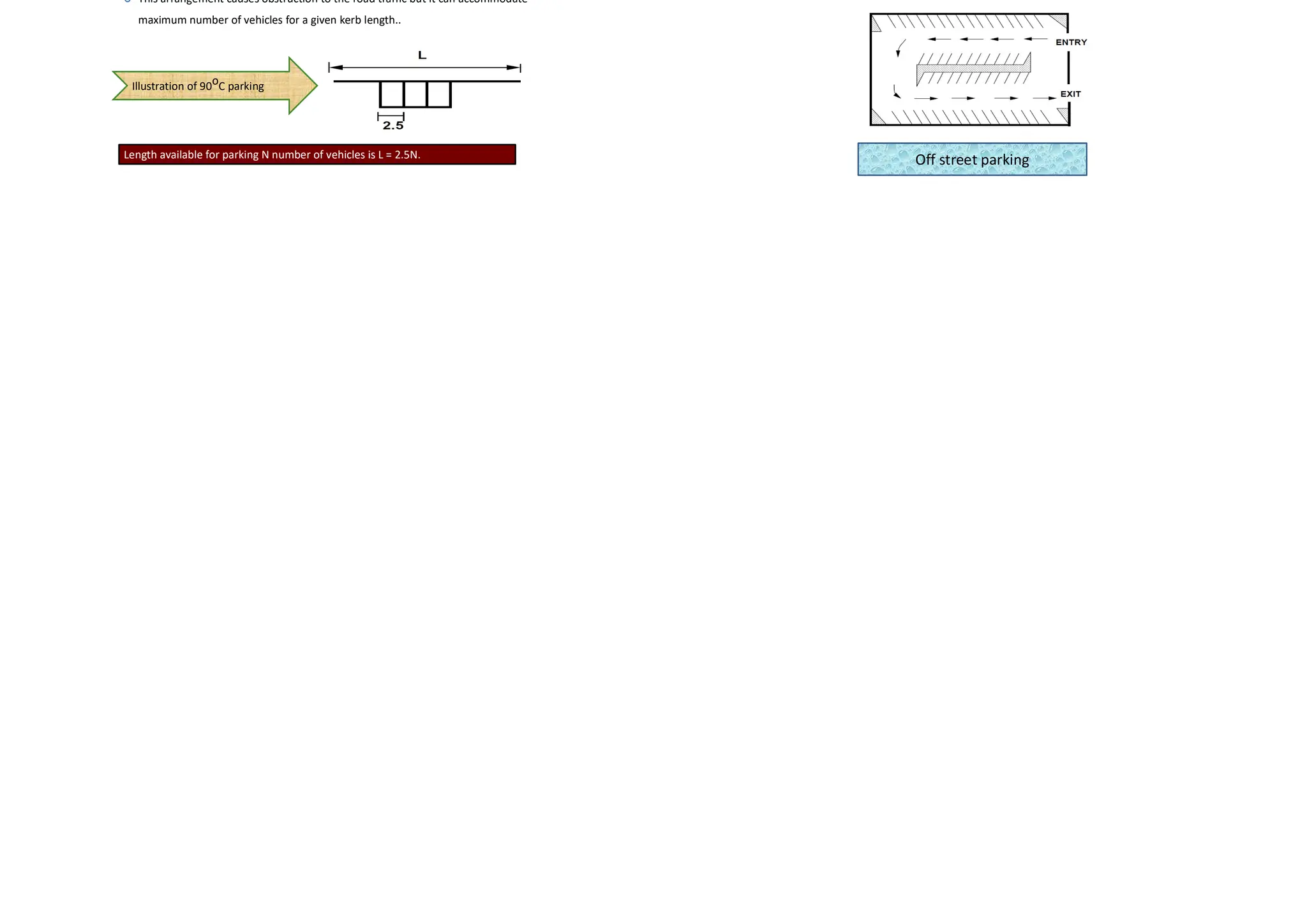
 This arrangement causes obstruction to the road traffic but it can accommodate
maximum number of vehicles for a given kerb length..
Illustration of 90oC parking
Length available for parking N number of vehicles is L = 2.5N.
• In many urban urban centres, some areas are exclusively allotted for
parking which will be at some distance away from the main stream of
traffic.
• Such a parking is referred to as off-street parking.
• They may be operated by either public agencies or private firms.
Off street parking
Off Street Parking

19. • From an in-out survey conducted for a parking area consisting of 40 bays, the initial
count was found to be 25.The number of vehicles coming in and out of the parking
lot for a time interval of 5 minutes is as shown in the table. Find the accumulation,
total parking load, average occupancy and efficiency of the parking lot
Example 1
• Accumulation can be found out as initial count plus number of vehicles that entered the parking lot till that time
minus the number of vehicles that just exited for that particular time interval. For the first time interval of 5 minutes,
accumulation can be found out as 25+3-2 = 26. It is being tabulated in column 4.
Solution
• Occupancy or parking index is given by equation For the
first time interval of five minutes, Parking index
=(26/40)*100 = 65%. The occupancy for the remaining time
slot is similarly calculated and is tabulated in column 5.
Avg. occupancy = Avg. of the occupancy values calculated
• Parking load is tabulated in column 6. It is obtained by
multiplying accumulation with the time interval. For the
first time interval, parking load = 26*5 = 130 vehicle
minutes.
• Total parking load is the summation of all the values in column 5 which is equal to 1935 vehicle minutes or 32.25 vehicle
hours
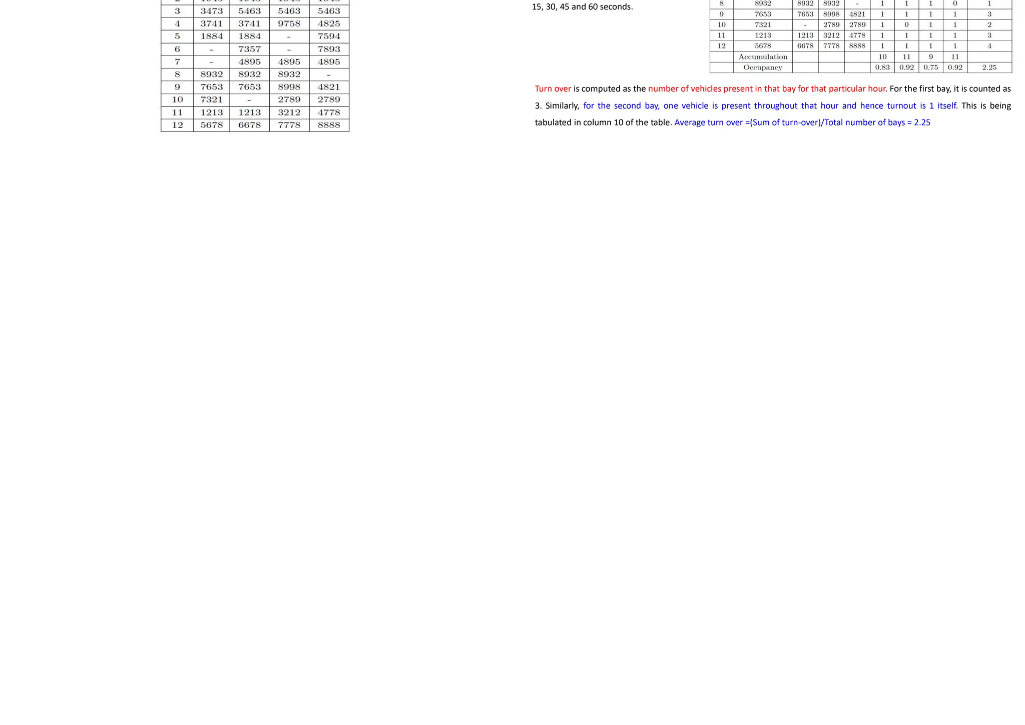
• The parking survey data collected from a parking lot by license plate method is s
shown in the table below. Find the average occupancy, average turn over, parking
load, parking capacity and efficiency of the parking lot.
Example 2 Cont…
Columns 1 to 5 is the input data. The
parking status in every bay is coded first.
If a vehicle occupies that bay for that time
interval, then it has a code 1. This is
shown in columns 6, 7, 8 and 9 of the
table corresponding to the time intervals
15, 30, 45 and 60 seconds.
Turn over is computed as the number of vehicles present in that bay for that particular hour. For the first bay, it is counted as
3. Similarly, for the second bay, one vehicle is present throughout that hour and hence turnout is 1 itself. This is being
tabulated in column 10 of the table. Average turn over =(Sum of turn-over)/Total number of bays = 2.25

20. • Accumulation for a time interval is the total of number of vehicles in the bays 1 to 12 for that time
interval. Accumulation for first time interval of 15 minutes = 1+1+1+1+1+0+0+1+1+1+1+1 = 10
Solution
• Parking volume = Sum of the turn over in all the bays = 27 vehicles
• Average duration is the average time for which the parking lot was used by the vehicles. It can be calculated
as sum of the accumulation for each time interval time interval divided by the parking volume
=((10+11+9+11)*15)/27 = 22.78 minutes/vehicle
Cont…
• Occupancy for that time interval is accumulation in that particular interval divided by total number of bays.
For first time interval of 15 minutes, occupancy = (10100)/12 = 83% Average occupancy is found out as the
average of total number of vehicles occupying the bay for each time interval. It is expressed in percentage.
Average occupancy = (0.83+0.92+0.75+0.92)/4*100 = 85.42%.
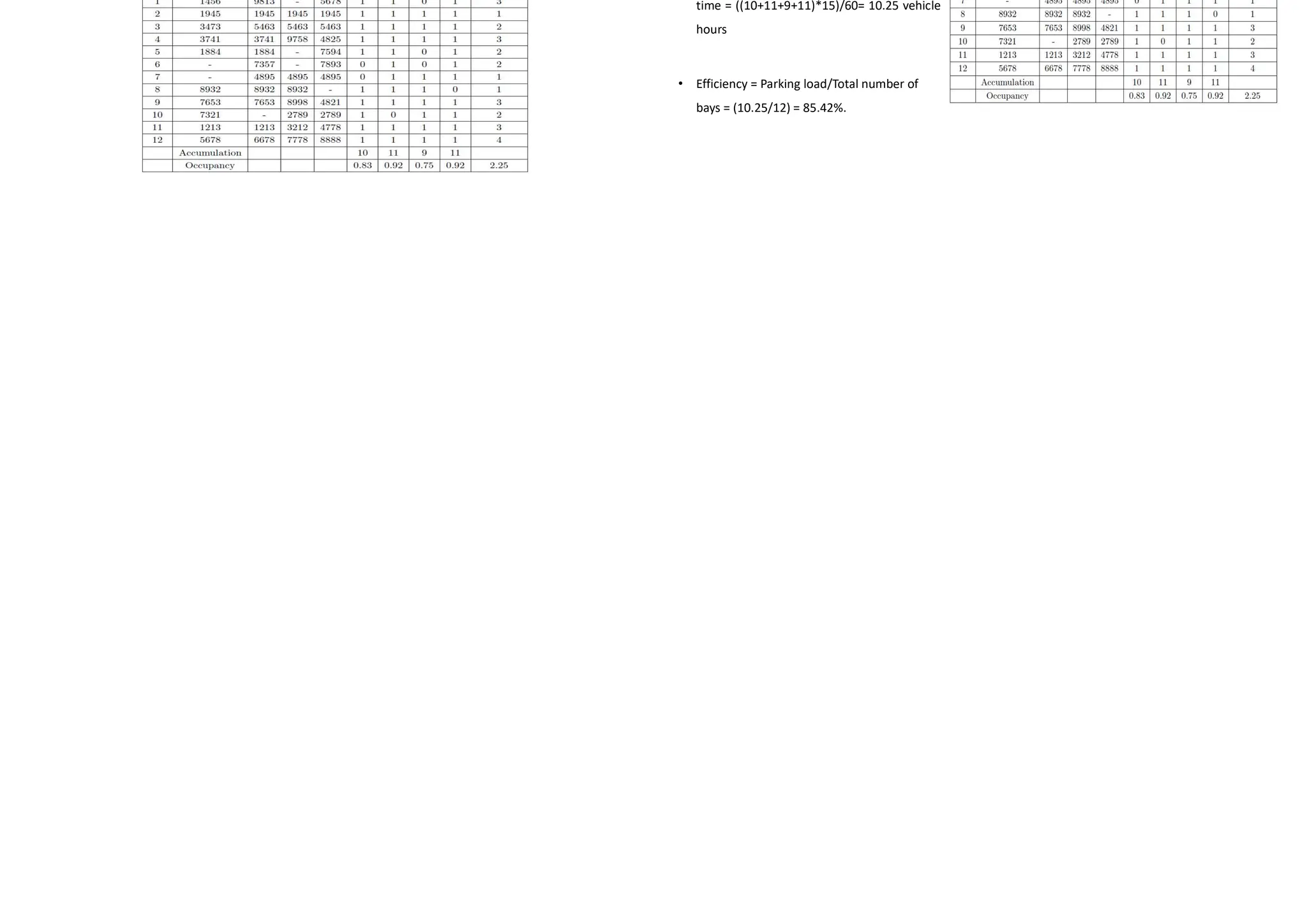
Cont…
• Parking capacity = number of bays number
of hours = 12*1 = 12 vehicle hours
• Parking load = total number of vehicles
accumulated at the end of each time interval
time = ((10+11+9+11)*15)/60= 10.25 vehicle
hours
• Efficiency = Parking load/Total number of
bays = (10.25/12) = 85.42%.
Cont…

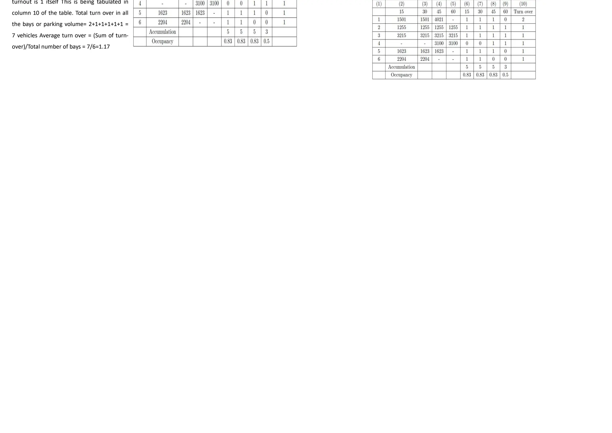
21. • The parking survey data collected from a parking lot by license plate
method is shown in table below. Find the average occupancy, average
turnover, parking load, parking capacity and efficiency of parking lot.
Example 3
• Column 1 to 5 is the input data. The parking status in every bay is coded first. If a vehicle occupies that bay
for that time interval, then it has a code 1. This is shown in columns 6, 7, 8 and 9 of the tables corresponding
to the time intervals 15,30,45 and 60 seconds.
Solution
• Turn over is computed as the number of
vehicles present in that bay for that particular
hour. For the first bay, it is counted as 2.
Similarly, for the second bay, one vehicle is
present throughout that hour and hence
turnout is 1 itself This is being tabulated in
column 10 of the table. Total turn over in all
the bays or parking volume= 2+1+1+1+1+1 =
7 vehicles Average turn over = (Sum of turn-
over)/Total number of bays = 7/6=1.17
Solution
• Average duration is the average time for which the parking lot was used by the vehicles. It can be
calculated as sum of the accumulation for each time interval time interval divided by the parking volume
=((5+5+5+3)*15)/7 = 38.57 minutes/vehicle.
• Average occupancy is found out as the average of total number of vehicles occupying the bay for each
time interval. It is expressed in percentage. Average occupancy =((0.83+0.83+0.83+0.5)/4)*100 = 75%.
Cont…

22. • Parking capacity = number of bays number of
hours = 6*1 = 6 vehicle hours
• Parking load = total number of vehicles
accumulated at the end of each time interval
time = (5+5+5+3)*15/60= 4.5 vehicle hours
• Efficiency = Parking load/Total number of
bays = 4.5/6 = 75%.
Cont…
TRAFFIC INTERSECTIONS
Introduction
Intersection is an area shared by two or more roads.
Its main function is to guide vehicles to their respective directions.
They are complex locations on any highway
Pedestrians also seek same place for crossing
Overall traffic flow depends on the performance of intersections
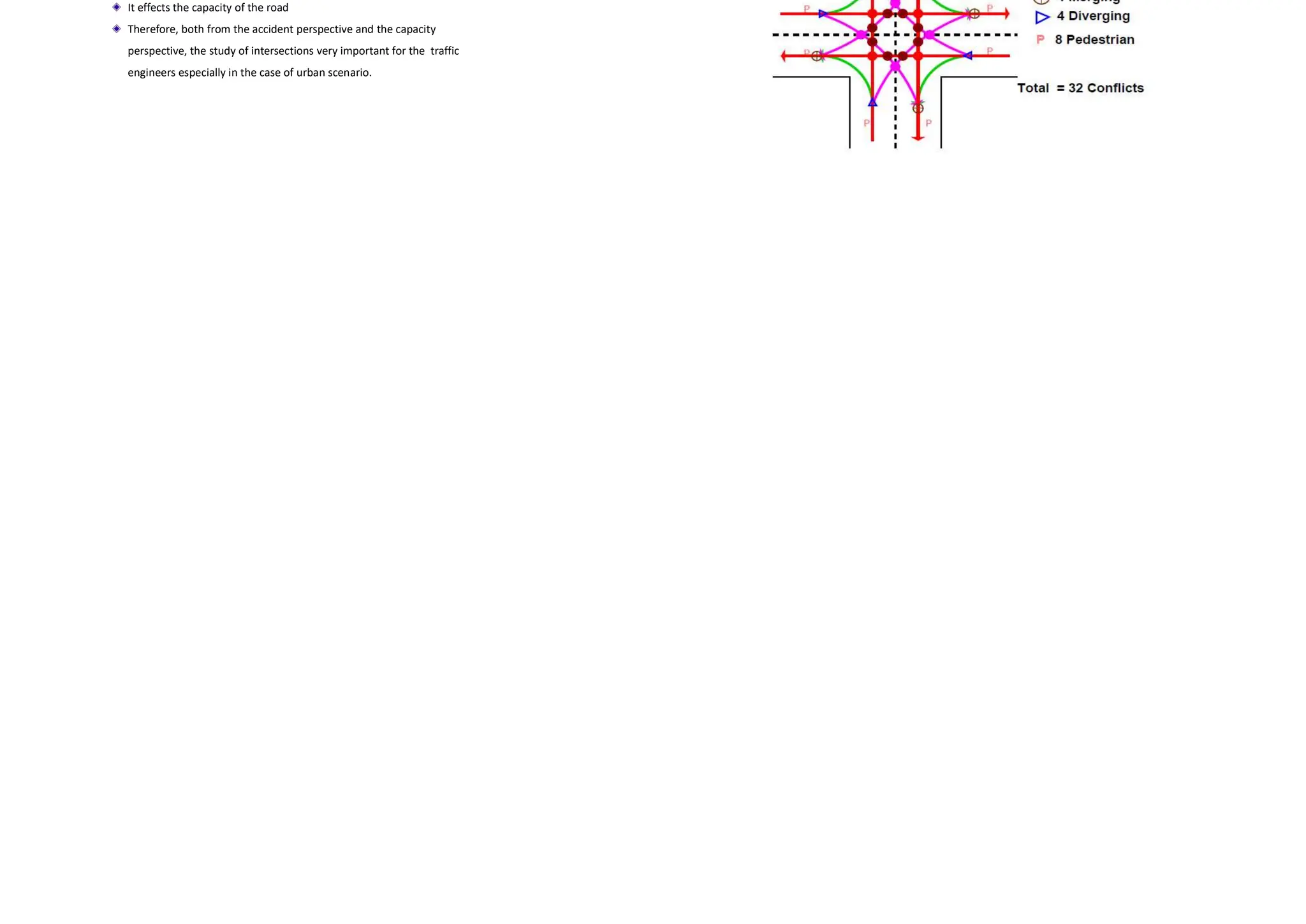
It effects the capacity of the road
Therefore, both from the accident perspective and the capacity
perspective, the study of intersections very important for the traffic
engineers especially in the case of urban scenario.
• They are different for different type of intersection.
• For example, at a four-legged intersection,
Conflicts at an intersection

23. • They are different for different type of intersection.
• For example, at a four-legged intersection,
Type of conflict No. of conflicts
Competing through movements 4
Right turn and movements 8
Right turn traffics 4
Left turn and merging traffics 4
Pedestrians 8
Diverging traffic 4
Total 32
Conflicts at an intersection Contd..
• The essence of the intersection control is to resolve these conflicts at the
intersection for the safe and efficient movement of both vehicular traffic
and pedestrians
 Time sharing
 Space sharing
 Traffic volume
 Road geometry
 Cost involved
 Importance of the road
.The type of intersection control that has to be adopted depends on
Levels of intersection control
The control of an intersection can be exercised at different levels.
o Passive control
o Semi control
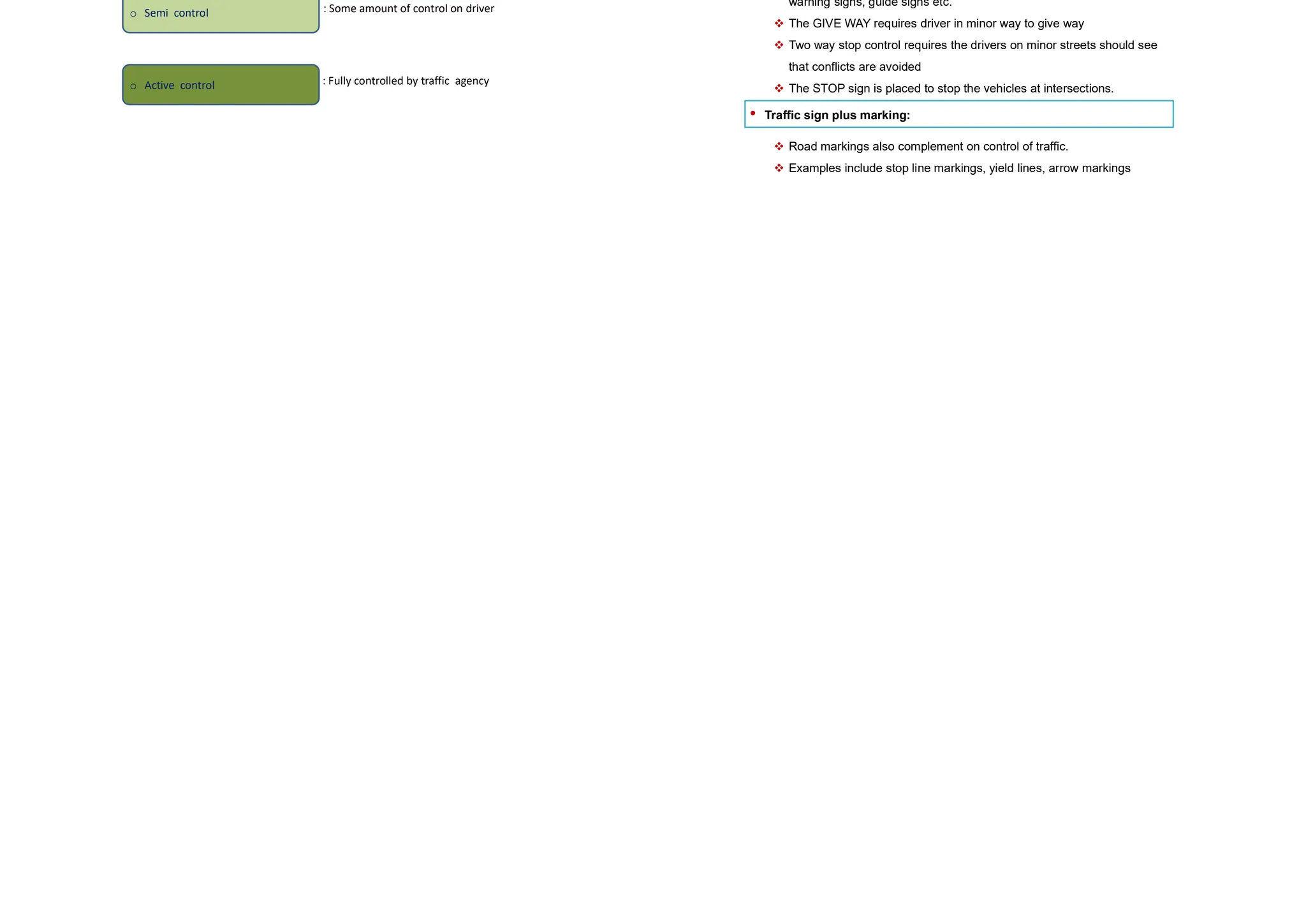
o Active control
: No explicit control on driver
: Some amount of control on driver
: Fully controlled by traffic agency
Passive control
• No control:
 Through movements will have more priority than turning
movements.
 The driver is expected to obey basic traffic rules
• Traffic signs:
 It is able to provide some level of control traffic with the help of
warning signs, guide signs etc.
 The GIVE WAY requires driver in minor way to give way
 Two way stop control requires the drivers on minor streets should see
that conflicts are avoided
 The STOP sign is placed to stop the vehicles at intersections.
• Traffic sign plus marking:
 Road markings also complement on control of traffic.
 Examples include stop line markings, yield lines, arrow markings

24. Semi control
• Channelization :
 The traffic is separated to flow through definite paths by raising a
portion of the road in the middle called as islands.
 The conflicts are reduced to great extend.
 The physical barrier is made possible with the help of some
barriers in road like traffic islands, road markings etc.
Channelization
Semi control contd..
• Traffic rotaries:
 The traffic is made to flow in one direction around a traffic island.
 All the severe conflicts are converted to mild conflicts.
 It is a form of at-grade intersection such that no through conflicts are there
 Merging, weaving and diverging operations reduce the conflicting movements at
the rotary.
Traffic rotaries
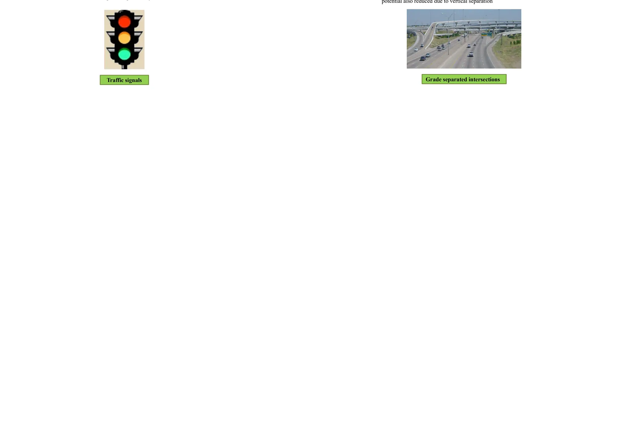
Active control
• Traffic signals :
 Control using traffic signal is based on time sharing approach.
 If more than two phases are provided it is called multiphase signal
 Fixed time signals and vehicle actuated signals are the most common modes .
 In fixed time signals, cycle time, phases and interval of each signal is fixed
 Vehicle actuated signals respond to dynamic traffic situations
Traffic signals
Active control contd..
• Grade separated intersections:
 They are of two types: at-grade intersections and grade separated intersections.
 In at-grade intersections all roads meet at a same vertical level.
 Grade-separated intersections allows the traffic to cross at different vertical levels
 These increase road capacity as vehicles will flow with high speed and accident
potential also reduced due to vertical separation
Grade separated intersections

25. Grade separated intersections
 Flyovers
o overpass and
o underpass
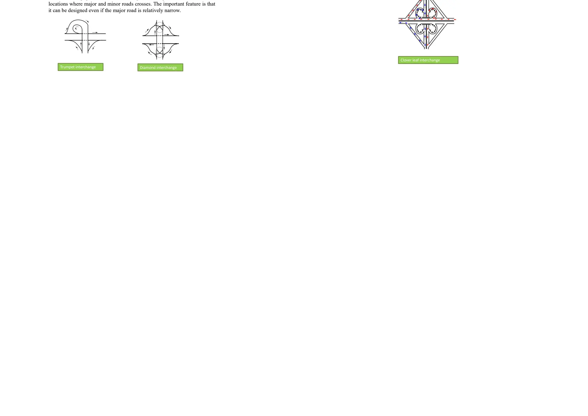
 Interchange
o Trumpet interchange
o Diamond interchange
o Clover leaf interchange
They are provided to separate the traffic in vertical direction.
Flyovers
Overpass
When two roads cross at a point, if the road having major traffic is
elevated to a higher grade for further movement of traffic, they are called
overpass
Overpass Underpass
 Underpass
If the major road is depressed to a lower level to cross another by means
of an under bridge or tunnel, it is called under-pass
Interchange
 Trumpet interchange
It is a popular form of three leg interchange. If one of the legs
of the interchange meets a highway at some angle but does not cross it, then the
interchange is called trumpet interchange.
 Diamond interchange
It is a popular form of four-leg interchange found in the urban
locations where major and minor roads crosses. The important feature is that
it can be designed even if the major road is relatively narrow.
Trumpet interchange Diamond interchange
Interchange contd..
 Clover leaf interchange
It is also a four leg interchange used when two highways of high volume
and speed intersect each other with considerable turning movements. The main
advantage is that it provides complete separation of traffic with achievement of high
speeds at intersections. However, the disadvantage is that large area of land is
required. Therefore, cloverleaf interchanges are provided mainly in rural areas
Clover leaf interchange

26. Channelized intersections
 Vehicles approaching an intersection are directed to definite paths by islands,
marking etc.
 They provides more safety and efficiency.
 It reduces the number of possible conflicts by reducing the area of conflicts
available in the carriageway.
 The presence of traffic islands, markings etc. forces the driver to reduce the
speed and becomes more cautious while maneuvering the intersection
 A channelizing island also serves as a refuge for pedestrians and makes
pedestrian crossing safer.
Channelization of traffic through
three-legged intersection
Channelization of traffic through
four-legged intersection
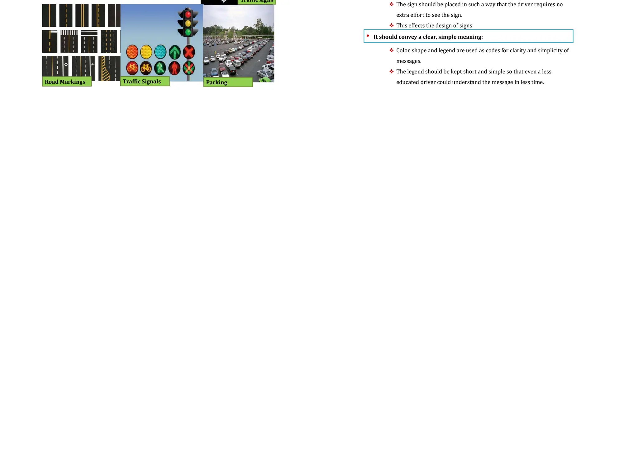
Road Markings
Over view
• The major types of traffic control devices used are
 Traffic signs,
 Road markings ,
 Traffic signals , and
 Parking control.
Traffic signs
Road Markings Traffic Signals Parking
Requirements of traffic control devices
• The control device should fulfill a need:
 Each device must have a specific purpose for the safe and efficient
operation of traffic flow
 The superfluous devices should not be used
• It should command attention from the road users:
 These signs should be properly visible distinctive and clear
 The sign should be placed in such a way that the driver requires no
extra effort to see the sign.
 This effects the design of signs.
• It should convey a clear, simple meaning:
 Color, shape and legend are used as codes for clarity and simplicity of
messages.
 The legend should be kept short and simple so that even a less
educated driver could understand the message in less time.

27. Cont…
• Road users must respect the signs:
 Respect is commanded only when the drivers are conditioned to
expect that all devices carry meaningful and important messages.
 Overuse, misuse and confusing messages of devices tends the drivers
to ignore them.
• The control device should provide adequate time for proper response
from the road users:
 This is again related to the design aspect of traffic control devices.
 The sign boards should be placed at a distance such that the driver
could see it and gets sufficient time to respond to the situation.
 For example, the STOP sign which is always placed at the stop line of
the intersection should be visible for atleast one safe stopping sight
distance away from the stop line.
Communicating Tools
• Color:
 Its first and most easily noticed characteristics of a device
 Colors like red, green, yellow, black, blue, and brown are used for different signs
 These are used to code certain devices and to reinforce specific messages
• Shape:
 It is the second element discerned by the driver next to the color of the device.
 Normally used shapes are circular, triangular, rectangular, and diamond shape.
Exceptional shapes
Octagonal
shape
Triangular
shape
Not used in India
Cont…
• Legend:
 the legend should be short, simple and specific so that it does not
divert the attention of the driver
 Symbols are normally used as legends so that even a person unable to
read the language will be able to understand that
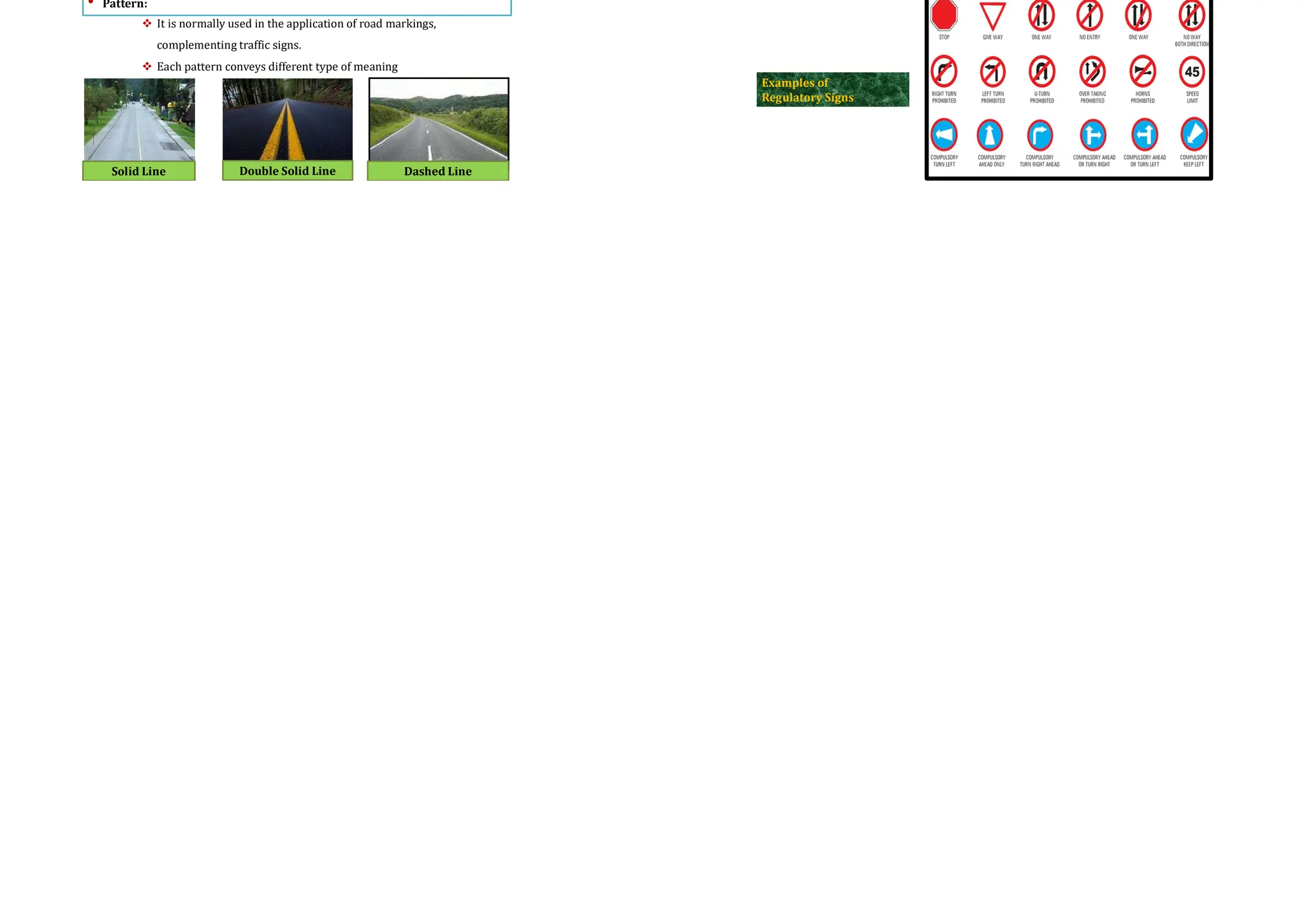
• Pattern:
 It is normally used in the application of road markings,
complementing traffic signs.
 Each pattern conveys different type of meaning
Solid Line Double Solid Line Dashed Line
Types of Traffic Signs
• Regulatory Signs / Mandatory Signs
Types of traffic Signs are:
 These signs are primarily meant for the safety of other road users.
 These signs have generally black legend on a white background.
 They are circular in shape with red borders.
Examples of
Regulatory Signs

28. Types of Traffic Signs Cont…
• Warning Signs / Cautionary signs
 These signs are for own safety of drivers
Examples of Warning Signs
Right Hand Bend Sign
 The legend will be black in color with white background.
 The shape used is upward triangle with red borders
Narrow Bridge
Sign
Rail way Crossing
Sign
Cont…
• Informative Signs / Guide signs
 They are provided to assist the drivers to reach their desired destinations.
 These are predominantly meant for the drivers who are unfamiliar to the place
Examples of Informative Signs
Route Markers Sign Destination
Sign
Mile posts Sign Service Center
Information
To Identify
numbered
highways
Indicate direction
to critical
destination points
Information
about the
progress along
the road
Provide information about
services such as food, fuel,
medical assistance etc.
Road Markings
 Purpose of road markings is to guide and control traffic on a highway
 They Supplement the function of traffic signs.
 Markings signify the delineation of traffic path and its lateral
clearance from traffic hazards for the safe movement of traffic
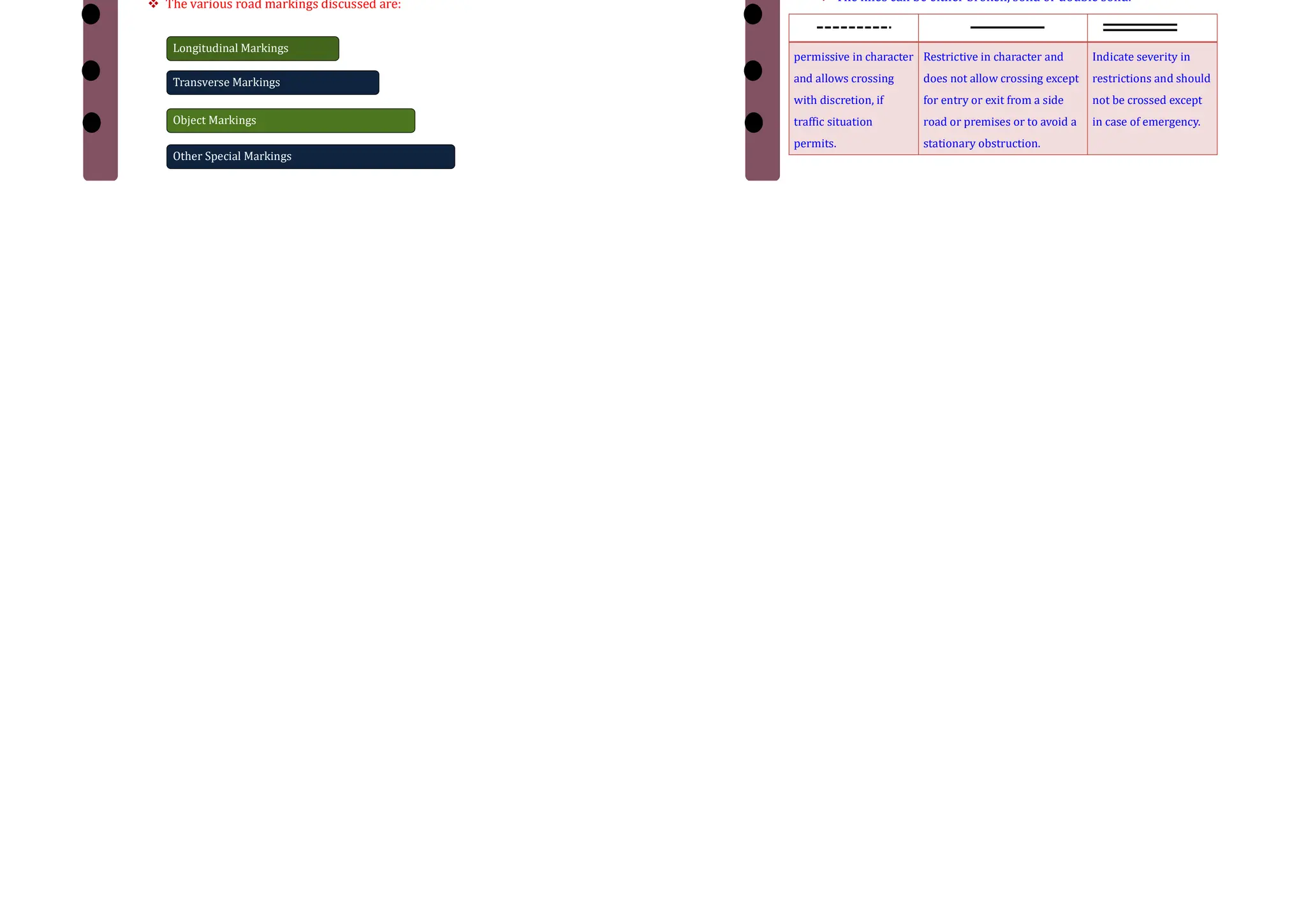
 The various road markings discussed are:
Longitudinal Markings
Transverse Markings
Object Markings
Other Special Markings
Longitudinal Markings
 Longitudinal markings are provided for separating traffic flow
White color used to separate traffic flow in same direction
Yellow color used to separate traffic flow in opposite
direction
Also to separate pavement edges
 The lines can be either broken, solid or double solid.
permissive in character
and allows crossing
with discretion, if
traffic situation
permits.
Restrictive in character and
does not allow crossing except
for entry or exit from a side
road or premises or to avoid a
stationary obstruction.
Indicate severity in
restrictions and should
not be crossed except
in case of emergency.

29. Types Of Longitudinal Markings
1. Central line
2. Traffic Lanes
3. No Passing Zones
4. Warning Lines
5. Border Or edge Lines
1. Central line
Central line marking for two lane road
 Center line is provided for roads having width less than 5 m and for
roads having more than four lanes
 The center line may be marked with either single broken line, single
solid line, double broken line, or double solid line depending upon
the road and traffic requirements.
1. On urban roads with less than four lanes, the center line may be single broken
line segments of 3 m long and 150 mm wide. The broken lines are placed with 4.5
m gaps
Cont…
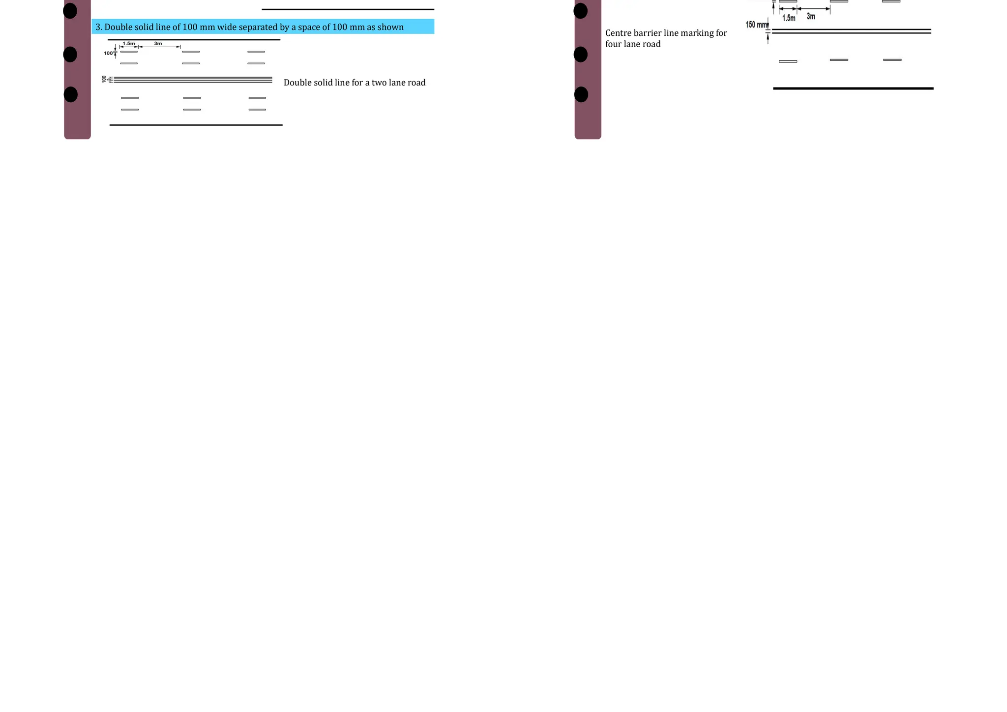
3. Double solid line of 100 mm wide separated by a space of 100 mm as shown
Centre line and lane marking for a
four lane road
2. On undivided urban roads with at least two traffic lanes in each direction, the centre
line marking may be a single solid line of 150 mm wide
Double solid line for a two lane road
Cont…
4. The centre barrier line marking for four lane road
Centre barrier line marking for
four lane road

30.  The subdivision of wide carriageways into separate lanes on
either side of the carriage way helps the driver to go straight
 At intersections, these traffic lane lines will eliminate confusion
and facilitates turning movements.
 The traffic lane lines are normally single broken lines of 100 mm
width
 Thus traffic lane markings help in increasing the capacity of the
road in addition ensuring more safety.
2. Traffic Lanes Over View
Lane marking for a four lane road
with solid barrier line
1. Lane marking for a four lane road with solid barrier line
2. Traffic lane marking for a four lane road with broken centre line
Traffic lane marking for a four
lane road with broken centre
line
3. No Passing Zones
 No passing zones are established on summit curves, horizontal
curves, and on two lane and three lane highways where overtaking
maneuvers are prohibited because of low sight distance
 It may be marked by a solid yellow line along the centre or a double
yellow line
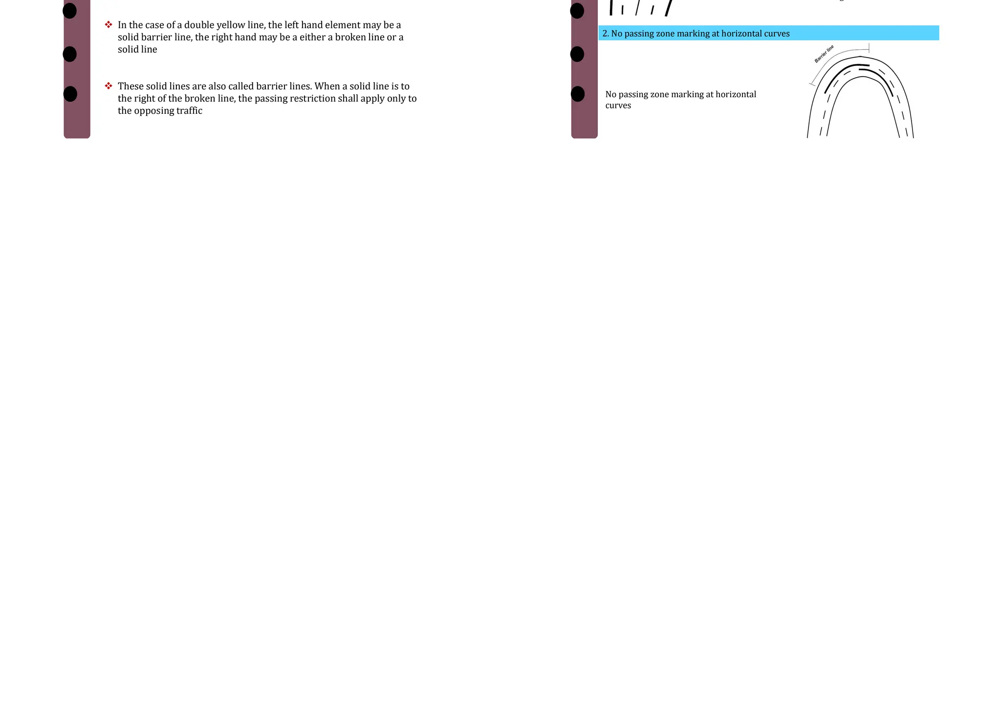
 In the case of a double yellow line, the left hand element may be a
solid barrier line, the right hand may be a either a broken line or a
solid line
 These solid lines are also called barrier lines. When a solid line is to
the right of the broken line, the passing restriction shall apply only to
the opposing traffic
Over View
1. Barrier line marking for a four lane road
Barrier line marking for a four lane road
2. No passing zone marking at horizontal curves
No passing zone marking at horizontal
curves

31. 4. Warning Lines
 Warning lines warn the drivers about the obstruction approaches.
 They are marked on horizontal and vertical curves where the visibility is
greater than prohibitory criteria specified for no overtaking zones.
 They are broken lines with 6 m length and 3 m gap.
 A minimum of seven line segments should be provided
1. Warning line marking for a two lane road
5. Border Or edge Lines
 Edge lines indicate edges of rural roads which have no kerbs to
delineate the limits up to which the driver can safely venture.
 They should be at least 150 mm from the actual edge of the
pavement.
 They are painted in yellow or white.
 All the lines should be preferably light reflective, so that they will be
visible during night also
Transverse Markings
 Transverse markings are marked across the direction of traffic
 They are marked at intersections
 The site conditions play a very important role. The type of road
marking for a particular intersection depends on several variables
such as speed characteristics of traffic, availability of space
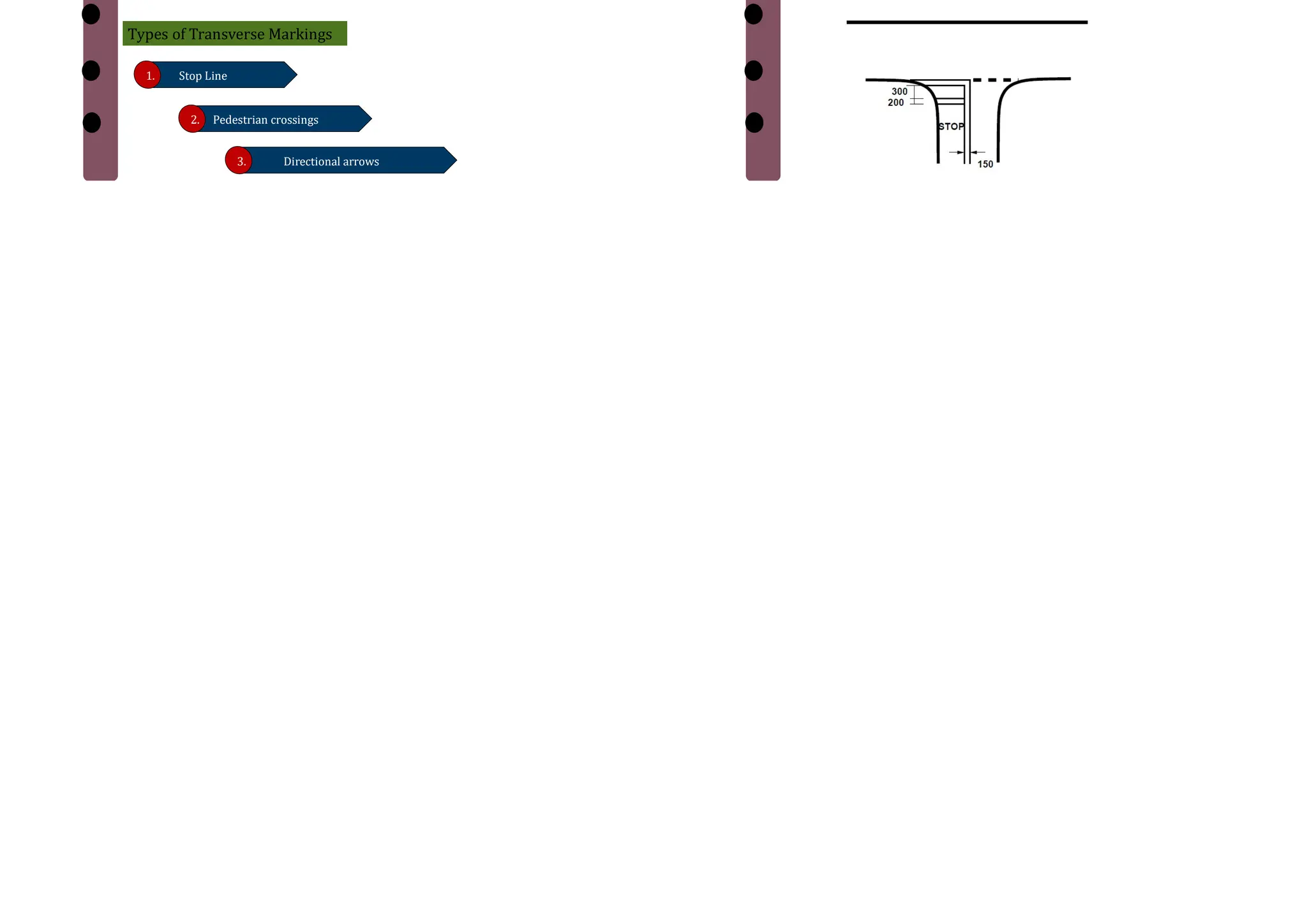
Types of Transverse Markings
1. Stop Line
2. Pedestrian crossings
3. Directional arrows
1. Stop Line
.
 Stop line indicates the position beyond which the vehicles should not proceed
when required to stop by control devices like signals or by traffic police.
 They should be placed either parallel to the intersecting roadway or at right
angles to the direction of approaching vehicles
1. Stop line marking near an intersection

32. 2. Pedestrian crossings
 The site should be selected that there is less inconvenience to the pedestrians
and also the vehicles are not interrupted too much.
 At intersections, the pedestrian crossings should be preceded by a stop line
at a distance of 2 to 3m for un-signalized intersections and at a distance of
one metre for signalized intersections.
 Most commonly used pattern for pedestrian crossing is Zebra crossing
consisting of equally spaced white strips of 500 mm wide.
1. Pedestrian marking near an intersection
3. Directional arrows
1. Directional arrow marking
 In addition to the warning lines on approaching lanes, directional arrows
should be used to guide the drivers in advance over the correct lane to be
taken while approaching busy intersections.
 Because of the low angle at which the markings are viewed by the drivers, the
arrows should be elongated in the direction of traffic for adequate visibility.
The dimensions of these arrows are also very important
Object Markings
 Physical obstructions in a carriageway like traffic island or obstructions near
carriageway like signal posts, pier etc. cause serious hazard to the flow of
traffic and should be adequately marked. They may be marked on the objects
adjacent to the carriageway.
Objects within the carriageway
1 Object Marking With in carriage way
 The obstructions within the carriageway such as traffic islands, raised
medians, etc. may be marked by not less than five alternate black and yellow
stripes.
 The stripes should slope forward at an angle of 45 with respect to the
direction of traffic. These stripes shall be uniform and should not be less than
100 m wide so as to provide sufficient visibility.
Cont…
 Objects(subway piers and abutments, culvert head walls etc.) adjacent to the
carriageway posing obstruction to the traffic flow)
 They should be marked with alternate black and white stripes at a forward
angle of 45 with respect to the direction of traffic.
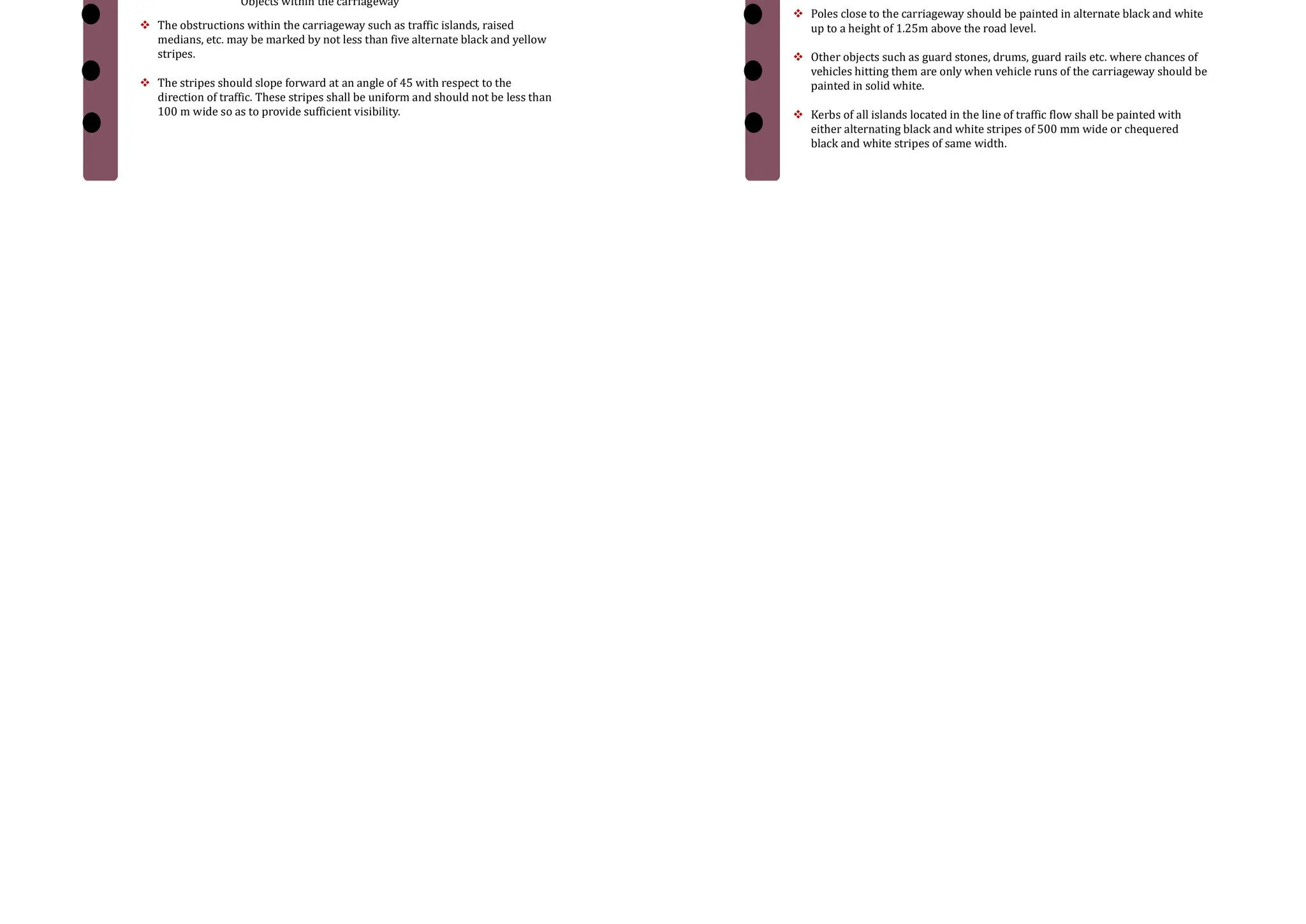
 Poles close to the carriageway should be painted in alternate black and white
up to a height of 1.25m above the road level.
 Other objects such as guard stones, drums, guard rails etc. where chances of
vehicles hitting them are only when vehicle runs of the carriageway should be
painted in solid white.
 Kerbs of all islands located in the line of traffic flow shall be painted with
either alternating black and white stripes of 500 mm wide or chequered
black and white stripes of same width.
2. Objects adjacent to carriageway

33. 1. Marking for objects adjacent to the road way
Cont… Word Messages
 Information to guide, regulate, or warn the road user may also be conveyed by
inscription of word message on road surface.
 Characters for word messages are usually capital letters. The legends should be as
brief as possible and shall not consist of more than three words for any message.
 Word messages require more and important time to read and comprehend than other
road markings. Therefore, only few and important ones are usually adopted.
 Some of the examples of word messages are STOP, SLOW, SCHOOL, RIGHT TUN ONLY
etc.
 The character of a road message is also elongated so that driver looking at the road
surface at a low angle can also read them easily.
Cont…
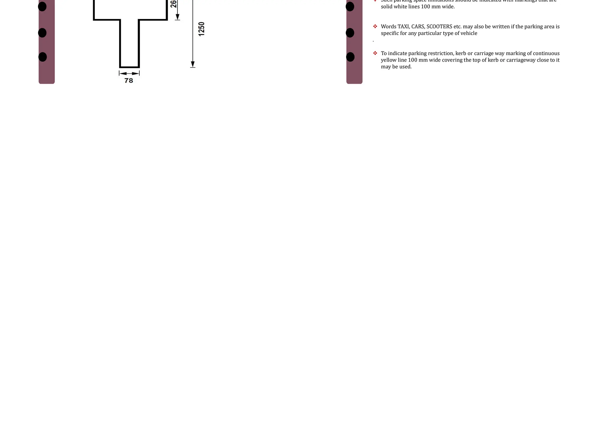
1. Typical dimension of the character T used in road marking
Parking
 The marking of the parking space limits on urban roads promotes more
efficient use of the parking spaces
 It tends to prevent encroachment on places like bus stops, fire hydrant zones
etc. where parking is undesirable.
 Such parking space limitations should be indicated with markings that are
solid white lines 100 mm wide.
 Words TAXI, CARS, SCOOTERS etc. may also be written if the parking area is
specific for any particular type of vehicle
.
 To indicate parking restriction, kerb or carriage way marking of continuous
yellow line 100 mm wide covering the top of kerb or carriageway close to it
may be used.

34. Hazardous Location
 Wherever there is a change in the width of the road, or any hazardous
location in the road, the driver should be warned about this situation with
the help of suitable road markings.
 Road markings showing the width transition in the carriageway should be of
100 mm width. Converging lines shall be 150 mm wide and shall have a taper
length of not less than twenty times the off-set distance.
In the figure, the driver is
warned about the position of the pier
through proper road markings.
1. Approach marking for obstructions on the road way