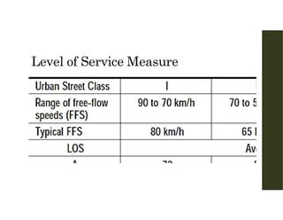
Measures of EffectivenessDefining
Levels of Service in HCM 2000
Measure of Effectiveness
Type of Facility
Type of Flow
Density [pc/mi/ln]
Density [pc/mi/ln]
Density [pc/mi/ln]
Density [pc/mi/ln]
Average Travel Speed [mi/hr]
Percent Time Spent Following [%]
Freeways
Basic sections
Weaving areas
Ramp junctions
Multilane Highways
Two-Lane Highways
Uninterrupted
Flow
Control Delay [s/veh]
Control Delay [s/veh]
Average Travel Speed [mi/hr]
Service Frequency [veh/day]
Service Headway [min]
Passengers/Seat
Space [ft2/ped]
Frequency of (Conflicting) Events [events/hr]
Signalized Intersections
Unsignalized Intersections
Urban Streets
Transit
Pedestrians
Bicycles
Interrupted
Flow
3.
Traffic Engineering Studies
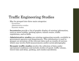
•May be grouped into three main categories:
Inventories
Administrative studies
Dynamic studies
• Inventories provide a list of graphic display of existing information,
such as street widths, parking spaces, transit routes, traffic
regulations, and so forth.
• Administrative studies use existing engineering records, available in
government agencies and departments. This information is used to
prepare an inventory of the relevant data such as results of surveys
which may involve field measurements and/or aerial photography.
• Dynamic traffic studies involve the collection of data under
operational conditions and include studies of speed, traffic volume,
travel time and delay, parking, and crashes (accidents).
4.
Dynamic Traffic Studies
•Spot Speed Studies are conducted to estimate the distribution of
speeds of vehicles in a stream of traffic at a particular location on
a highway. The speed of a vehicle is defined as the rate of
movement of the vehicle; it is usually expressed in kilometers per
hour (kph).
5.
Purpose of SpotSpeed Studies
• Establish parameters for traffic operation and control,
such as speed zones, speed limits (85th – percentile
speed is commonly used as the speed limit on a road),
and passing restrictions.
• Evaluate the effectiveness of traffic control devices,
such as variable message signs at work zones
• Monitor the effect of speed enforcement programs, such
as the use of drone radar and the use of differential
speed limits for passenger cars and trucks.
6.
Purpose of SpotSpeed Studies
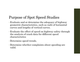
• Evaluate and or determine the adequacy of highway
geometric characteristics, such as radii of horizontal
curves and lengths of vertical curves.
• Evaluate the effect of speed on highway safety through
the analysis of crash data for different speed
characteristics
• Determine speed trends.
• Determine whether complaints about speeding are
valid.
7.
Location for SpotSpeed Studies
• Location that represent different traffic conditions on a
highway or highways are used for basic data collection.
• Mid-blocks of urban highways and straight, level
sections of rural highways are sites for speed trend
analyses.
• Any location may be used for the solution of a specific
traffic engineering problem.
8.
Methods for ConductingSpot Speed
Studies
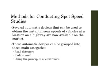
• Several automatic devices that can be used to
obtain the instantaneous speeds of vehicles at a
location on a highway are now available on the
market.
• These automatic devices can be grouped into
three main categories:
Road detectors
Radar-based
Using the principles of electronics
9.
Road Detectors
• Thesedevices can be used to collect data on speeds at
the same time as volume data are being collected.
• When road detectors are used to measure speed, they
should be laid such that the probability of a passing
vehicle closing the connection of the meter during a
speed measurement is reduced to a minimum. This is
achieved by separating the road detectors by a distance
of 3 to 15 ft.
• The advantage of the detector meters is that human
errors are considerably reduced.
10.
Road Detectors
• Pneumaticroad tubes are laid across the lane in which
data are to be collected. When a moving vehicle passes
over the tube, an air impulse is transmitted through the
tube to the counter. When used for speed
measurements, two tubes are placed across the lane,
usually about 6 ft apart.
11.
Road Detectors
• Animpulse is recorded when the front wheels of a
moving vehicle pass over the first tube; shortly
afterward a second impulse is recorded when the front
wheels pass over the second tube. The time elapsed
between the two impulses and the distance between the
tubes are used to compute the speed of the vehicle.
12.
Road Detectors
• Aninductive loop is a rectangular
wire loop buried under the
roadway surface. It usually serves
as the detector of a resonant
circuit. It operates on the principle
that a disturbance in the electrical
field is created when a motor
vehicle passes across it. This
causes a change in potential that
is amplified, resulting in an
impulse being sent to the counter.
13.
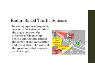
Radar-Based Traffic Sensors
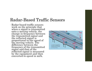
•Radar-based traffic sensors
work on the principle that
when a signal is transmitted
onto a moving vehicle, the
change in frequency between
the transmitted signal and
the reflected signal is
proportional to the speed of
the moving vehicle. The
difference between the
frequency of the transmitted
signal and that of the
reflected signal is measured
by the equipment and then
converted to speed in mi/h.
14.
Radar-Based Traffic Sensors
•The advantage of this
method is that because
pneumatic tubes are not
used, if the equipment can
be located at an
inconspicuous position, the
influence on driver
behavior is considerably
reduced.
15.
Radar-Based Traffic Sensors
•In setting up the equipment,
care must be taken to reduce
the angle between the
direction of the moving
vehicle and the line joining
the center of the transmitter
and the vehicle. The value of
the speed recorded depends
on that angle.
16.
Radar-Based Traffic Sensors
•If the angle is not zero, an
error related to the cosine of
that angle is introduced,
resulting in a lower speed
than that which would have
been recorded if the angle
had been zero. However, this
error is not very large,
because the cosines of small
angles are not much less
than one.
17.
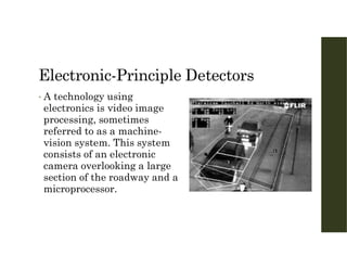
Electronic-Principle Detectors
• Atechnology using
electronics is video image
processing, sometimes
referred to as a machine-
vision system. This system
consists of an electronic
camera overlooking a large
section of the roadway and a
microprocessor.
18.
Electronic-Principle Detectors
• Theelectronic camera
receives the images from the
road; the microprocessor
determines the vehicle’s
presence or passage. This
information is then used to
determine the traffic
characteristics in real time.
19.
Important Speed Characteristics
•Average Speed – the arithmetic mean of all observed vehicle
speeds (which is the sum of all spot speeds divided by the number
of recorded speeds
• Standard Deviation of Speeds – a measure of the spread of
the individual speeds
• The ith-percentile Spot Speed - the spot speed value below
which i percent of the vehicles travel; for example, 85th-
percentile spot speed is the speed below which 85 percent of the
vehicles travel and above which 15 percent of the vehicles travel.
20.
Important Speed Characteristics
•Median Speed - the speed at the middle value in a series of spot
speeds that are arranged in ascending order. 50 percent of the
speed values will be greater than the median; 50 percent will be
less than the median.
• Modal Speed - the speed value that occurs most frequently in a
sample of spot speeds.
• Pace - the range of speed – usually taken at 10 kph intervals –
that has the greatest number of observations. For example, if a
set of speed data includes speeds between 30-60 kph, the speed
intervals will be 30 to 40 kph, 40 to 50 kph, and 50 to 60 kph,
assuming a range of 10 kph. The pace is 40 to 50 kph if this
range of speed has the highest number of observations.
21.
Important Speed Characteristics
•Average Speed
where u = arithmetic mean
ui = speed of the ith vehicle / midvalue of the
ith speed group
N = number of observed values
fi = number of observations in each speed
group
22.
Important Speed Characteristics
•Standard Deviation of Speeds
∑ ∑
∑
whereSD = standard deviation
u = arithmetic mean
uj = jth observation
N = number of observations
fi = frequency of speed class i
ui = midvalue of speed class i
23.
Speed class (kph)Class midvalue, ui
Class frequency (no. of
observations in class), fi fi * ui fi * (ui-u)^2
35-39.99 37.5 7 262.5 963.9212828
40-44.99 42.5 19 807.5 861.7659309
45-49.99 47.5 29 1377.5 87.26572262
50-54.99 52.5 24 1260 255.8933778
55-59.99 57.5 14 805 956.4139942
60-64.99 62.5 5 312.5 879.8417326
Total 98 4825 4005.102041
Mean 49.23469388
SD 6.425707102
Example 1
𝜇̅ =
∑ 𝑓 𝜇
∑ 𝑓
𝑆𝐷 =
∑ 𝑓 𝜇 − 𝜇
∑ 𝑓 − 1
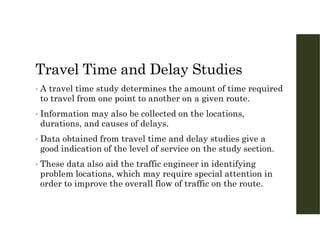
Travel Time andDelay Studies
• A travel time study determines the amount of time required
to travel from one point to another on a given route.
• Information may also be collected on the locations,
durations, and causes of delays.
• Data obtained from travel time and delay studies give a
good indication of the level of service on the study section.
• These data also aid the traffic engineer in identifying
problem locations, which may require special attention in
order to improve the overall flow of traffic on the route.
26.
Application for TravelTime and
Delay Data
• May be used in the ff:
Determination of the efficiency of a route with respect
to its ability to carry traffic
Identification of locations with relatively high delays
and the causes for those delays
Performance of before-and-after studies to evaluate
the effectiveness of traffic operation improvements
27.
Application for TravelTime and
Delay Data
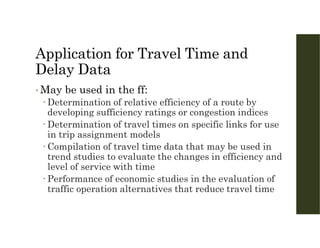
• May be used in the ff:
Determination of relative efficiency of a route by
developing sufficiency ratings or congestion indices
Determination of travel times on specific links for use
in trip assignment models
Compilation of travel time data that may be used in
trend studies to evaluate the changes in efficiency and
level of service with time
Performance of economic studies in the evaluation of
traffic operation alternatives that reduce travel time
28.
Commonly Used TermsRelated to
Time and Delay Studies
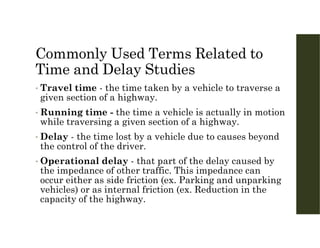
• Travel time - the time taken by a vehicle to traverse a
given section of a highway.
• Running time - the time a vehicle is actually in motion
while traversing a given section of a highway.
• Delay - the time lost by a vehicle due to causes beyond
the control of the driver.
• Operational delay - that part of the delay caused by
the impedance of other traffic. This impedance can
occur either as side friction (ex. Parking and unparking
vehicles) or as internal friction (ex. Reduction in the
capacity of the highway.
29.
Commonly Used TermsRelated to
Time and Delay Studies
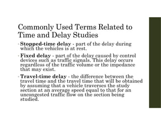
• Stopped-time delay - part of the delay during
which the vehicles is at rest.
• Fixed delay - part of the delay caused by control
devices such as traffic signals. This delay occurs
regardless of the traffic volume or the impedance
that may exist.
• Travel-time delay - the difference between the
travel time and the travel time that will be obtained
by assuming that a vehicle traverses the study
section at an average speed equal to that for an
uncongested traffic flow on the section being
studied.
30.
Travel Time andDelay Studies
• Methods Requiring a Test Vehicle
1. Floating-Car Technique
2. Average-Speed Technique
3. Moving-Vehicle Technique
• Methods Not Requiring a Test Vehicle
1. License-Plate Observations
2. Interviews
3. ITS Advanced Technologies
31.
Floating-Car Technique
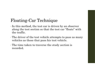
• Inthis method, the test car is driven by an observer
along the test section so that the test car “floats” with
the traffic.
• The driver of the test vehicle attempts to pass as many
vehicles as those that pass his test vehicle.
• The time taken to traverse the study section is
recorded.
Floating-Car Technique
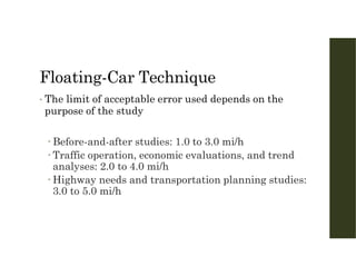
• Thelimit of acceptable error used depends on the
purpose of the study
Before-and-after studies: 1.0 to 3.0 mi/h
Traffic operation, economic evaluations, and trend
analyses: 2.0 to 4.0 mi/h
Highway needs and transportation planning studies:
3.0 to 5.0 mi/h
34.
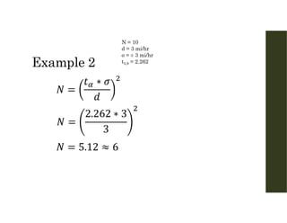
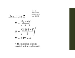
Example 2
• Anengineer, wishing to determine the travel time and average
speed along a section of an urban highway as part of an annual
trend analysis on traffic operations, conducted a travel time
study using the floating-car technique. He carried out 10 runs
and obtained a standard deviation of ±3 mi/h in the speeds
obtained. If a 5% significance level is assumed, is the number of
test runs adequate?
Example 2
N =10
d = 3 mi/hr
σ = ± 3 mi/hr
t5,9 = 2.262
37.
Example 2
N =10
d = 3 mi/hr
σ = ± 3 mi/hr
t5,9 = 2.262
38.
Example 2
N =10
d = 3 mi/hr
σ = ± 3 mi/hr
t5,9 = 2.262
The number of runs
carried out are adequate
39.
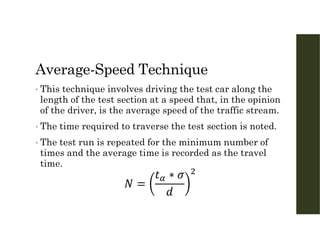
Average-Speed Technique
• Thistechnique involves driving the test car along the
length of the test section at a speed that, in the opinion
of the driver, is the average speed of the traffic stream.
• The time required to traverse the test section is noted.
• The test run is repeated for the minimum number of
times and the average time is recorded as the travel
time.
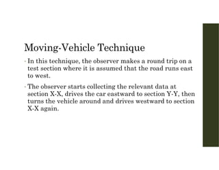
Moving-Vehicle Technique
• Inthis technique, the observer makes a round trip on a
test section where it is assumed that the road runs east
to west.
• The observer starts collecting the relevant data at
section X-X, drives the car eastward to section Y-Y, then
turns the vehicle around and drives westward to section
X-X again.
43.
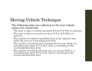
Moving-Vehicle Technique
• Thefollowing data are collected as the test vehicle
makes the round trip
The time it takes to travel east from X-X to Y-Y (Te), in minutes
The time it takes to travel west from Y-Y to X-X (Tw), in
minutes
The number of vehicles travelling west in the opposite lane
while the test car is travelling east (Ne)
The number of vehicles that overtake the test car while it is
travelling west from Y-Y to X-X, that is, travelling in the
westbound direction (Ow)
The number of vehicles that the test car passes while it is
travelling west from Y-Y to X-X, that is, travelling in the
westbound direction (Pw)
44.
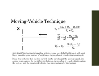
Moving-Vehicle Technique
• Notethat if the test car is traveling at the average speed of all vehicles, it will most
likely pass the same number of vehicles as the number of vehicles that overtake it
• Since it is probable that the test car will not be traveling at the average speed, the
second term corrects for the difference between the number of vehicles that overtake
the test car and the number of vehicles that are overtaken by the test car
45.
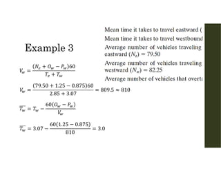
Example 3
• Thefollowing data were obtained in a travel time study on a
section of highway using the moving-vehicle technique.
Determine the travel time and volume in each direction at this
section of the highway.
Travel Time andDelay Studies
• Methods Requiring a Test Vehicle
1. Floating-Car Technique
2. Average-Speed Technique
3. Moving-Vehicle Technique
• Methods Not Requiring a Test Vehicle
1. License-Plate Observations
2. Interviews
3. ITS Advanced Technologies
52.
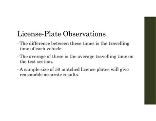
License-Plate Observations
• Thelicense-plate method requires that observers be
positioned at the beginning and end of the test section.
• Observers also can be positioned at other locations if
elapsed times to those locations are required. Each
observer records the last three or four digits of the
license plate of each car that passes, together with the
time at which the car passes.
• The reduction of the data is accomplished in the office
by matching the times of arrival at the beginning and
end of the test section for each license plate recorded.
53.
License-Plate Observations
• Thedifference between these times is the travelling
time of each vehicle.
• The average of these is the average travelling time on
the test section.
• A sample size of 50 matched license plates will give
reasonable accurate results.
54.
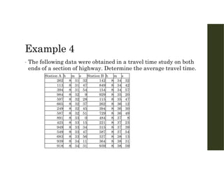
Example 4
• Thefollowing data were obtained in a travel time study on both
ends of a section of highway. Determine the average travel time.
s
m
h
Station B
s
m
h
Station A
32
34
8
142
32
31
8
262
42
34
8
849
47
31
8
113
57
34
8
154
54
31
8
394
20
35
8
929
9
32
8
984
47
35
8
115
28
32
8
597
12
36
8
262
37
32
8
665
30
36
8
394
45
32
8
249
49
36
8
729
51
32
8
587
8
37
8
484
0
33
8
891
23
37
8
221
15
33
8
425
39
37
8
315
34
33
8
949
54
37
8
587
47
33
8
549
13
38
8
337
56
33
8
683
31
38
8
364
11
34
8
939
59
38
8
939
31
34
8
918
55.
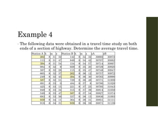
Example 4
• Thefollowing data were obtained in a travel time study on both
ends of a section of highway. Determine the average travel time.
sB
sA
s
m
h
Station B
s
m
h
Station A
30872
30692
32
34
8
142
32
31
8
262
30882
30707
42
34
8
849
47
31
8
113
30897
30714
57
34
8
154
54
31
8
394
30920
30729
20
35
8
929
9
32
8
984
30947
30748
47
35
8
115
28
32
8
597
30972
30757
12
36
8
262
37
32
8
665
30990
30765
30
36
8
394
45
32
8
249
31009
30771
49
36
8
729
51
32
8
587
31028
30780
8
37
8
484
0
33
8
891
31043
30795
23
37
8
221
15
33
8
425
31059
30814
39
37
8
315
34
33
8
949
31074
30827
54
37
8
587
47
33
8
549
31093
30836
13
38
8
337
56
33
8
683
31111
30851
31
38
8
364
11
34
8
939
31139
30871
59
38
8
939
31
34
8
918
56.
Example 4
• Thefollowing data were obtained in a travel time study on both
ends of a section of highway. Determine the average travel time.
sB
sA
s
m
h
Station B
s
m
h
Station A
30872
30692
32
34
8
142
32
31
8
262
30882
30707
42
34
8
849
47
31
8
113
30897
30714
57
34
8
154
54
31
8
394
30920
30729
20
35
8
929
9
32
8
984
30947
30748
47
35
8
115
28
32
8
597
30972
30757
12
36
8
262
37
32
8
665
30990
30765
30
36
8
394
45
32
8
249
31009
30771
49
36
8
729
51
32
8
587
31028
30780
8
37
8
484
0
33
8
891
31043
30795
23
37
8
221
15
33
8
425
31059
30814
39
37
8
315
34
33
8
949
31074
30827
54
37
8
587
47
33
8
549
31093
30836
13
38
8
337
56
33
8
683
31111
30851
31
38
8
364
11
34
8
939
31139
30871
59
38
8
939
31
34
8
918
57.
Example 4
• Thefollowing data were obtained in a travel time study on both
ends of a section of highway. Determine the average travel time.
sB
sA
s
m
h
Station B
s
m
h
Station A
30972
30692
12
36
8
262
32
31
8
262
30990
30714
30
36
8
394
54
31
8
394
31074
30771
54
37
8
587
51
32
8
587
31139
30851
59
38
8
939
11
34
8
939
58.
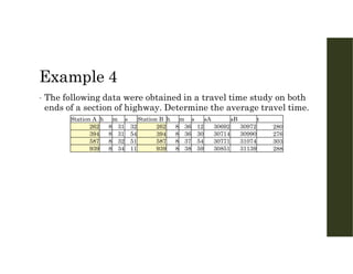
Example 4
• Thefollowing data were obtained in a travel time study on both
ends of a section of highway. Determine the average travel time.
t
sB
sA
s
m
h
Station B
s
m
h
Station A
280
30972
30692
12
36
8
262
32
31
8
262
276
30990
30714
30
36
8
394
54
31
8
394
303
31074
30771
54
37
8
587
51
32
8
587
288
31139
30851
59
38
8
939
11
34
8
939
59.
Example 4
• Thefollowing data were obtained in a travel time study on both
ends of a section of highway. Determine the average travel time.
t
sB
sA
s
m
h
Station B
s
m
h
Station A
280
30972
30692
12
36
8
262
32
31
8
262
276
30990
30714
30
36
8
394
54
31
8
394
303
31074
30771
54
37
8
587
51
32
8
587
288
31139
30851
59
38
8
939
11
34
8
939
286.75
Average
60.
Interviews
• The interviewingmethod is carried out by obtaining
information from people who drive on the study site
regarding their travel times, their experience of delays,
and so forth.
• This method facilitates the collection of a large amount
of data in a relatively short time.
• However, it requires the cooperation of the people
contacted, since the result depends entirely on the
information given by them.
61.
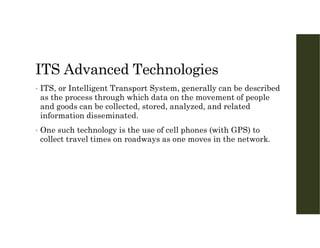
ITS Advanced Technologies
•ITS, or Intelligent Transport System, generally can be described
as the process through which data on the movement of people
and goods can be collected, stored, analyzed, and related
information disseminated.
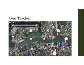
• One such technology is the use of cell phones (with GPS) to
collect travel times on roadways as one moves in the network.
Volume Studies
• Conductedto collect data on the number of vehicles
and/or pedestrians that pass a point on a highway
facility during a specified time period.
• Time periods vary from as little as 15 minutes to as
much as a year depending on the anticipated use of the
data
• The data collected also may be put into subclasses
which may include directional movement, occupancy
rates, vehicle classification, and pedestrian age
66.
Important Volume Characteristics
•Average Weekday Traffic (AWT) – average 24-hour
weekday volume at a given location over a defined time
period less than one year
• Average Daily Traffic (ADT) – average 24-hour
volume at a given location over a defined time period
less than one year
• Average Annual Weekday Traffic (AAWT) –
average 24-hour volume occurring on weekdays over a
full 365-day year
• Average Annual Daily Traffic (AADT) – average 24-
hour volume at a given location over a full 365-day year
Important Volume Characteristics
•Peak Hour Volume (PHV) – the maximum number of
vehicles that pass a point on a highway during a period
of 60 consecutive minutes
• Vehicle Classification (VC) – records volume with
respect to the type of vehicles, for example, passenger
cars, two-axle trucks, or three-axle trucks
• Vehicle Miles of Travel (VMT) – a measure of travel
along a section of road. It is the product of the traffic
volume (that is, average weekday volume or ADT) and
the length of roadway in miles to which the volume is
applicable.
69.
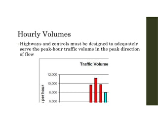
Hourly Volumes
• Dailyvolumes can not be used alone for design or
operational analysis purposes.
• Volume varies over the 24 hours of the day, with the
maximum flow occurring during the morning and
evening commuter “rush hours.”
• The single hour of the day with the highest hourly
volume is referred to as the peak hour.
Design
Operational analysis
70.
Hourly Volumes
• Highwaysand controls must be designed to adequately
serve the peak-hour traffic volume in the peak direction
of flow
71.
Subhourly Volumes andRates of
Flow
• The variation of traffic within a given hour is
also of considerable interest.
• A facility may have sufficient capacity to serve
the peak-hour demand, but short-term peaks of
flow within the hour may exceed capacity and
create a breakdown.
• Volumes observed for periods of less than one
hour are generally expressed as equivalent
hourly rates of flow.
72.
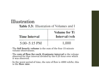
Illustration
• The fullhourly volume is the sum of the four 15-minute
volume observations.
• The rate of flow for each 15-minute interval is the volume
observed for that interval divided by the 0.25 hour over which
it was observed.
• In the worst period of time, the rate of flow is 4800 veh/hr, this
is the flow rate.
73.
Methods of ConductingVolume
Counts
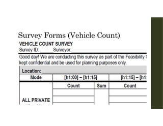
• Manual Method
Manual method involves one or more persons recording observed vehicles using a
counter.
With this type of counter, both the turning movements at the intersection and the
types of vehicles can be recorded.
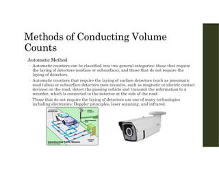
Methods of ConductingVolume
Counts
• Automatic Method
Automatic counters can be classified into two general categories: those that require
the laying of detectors (surface or subsurface), and those that do not require the
laying of detectors.
Automatic counters that require the laying of surface detectors (such as pneumatic
road tubes) or subsurface detectors (non invasive, such as magnetic or electric contact
devices) on the road, detect the passing vehicle and transmit the information to a
recorder, which is connected to the detector at the side of the road.
Those that do not require the laying of detectors use one of many technologies
including electronics: Doppler principles, laser scanning, and infrared.
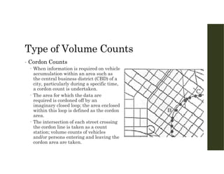
Type of VolumeCounts
• Cordon Counts
When information is required on vehicle
accumulation within an area such as
the central business district (CBD) of a
city, particularly during a specific time,
a cordon count is undertaken.
The area for which the data are
required is cordoned off by an
imaginary closed loop; the area enclosed
within this loop is defined as the cordon
area.
The intersection of each street crossing
the cordon line is taken as a count
station; volume counts of vehicles
and/or persons entering and leaving the
cordon area are taken.
80.
Type of VolumeCounts
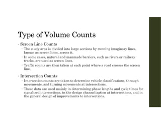
• Screen Line Counts
The study area is divided into large sections by running imaginary lines,
known as screen lines, across it.
In some cases, natural and manmade barriers, such as rivers or railway
tracks, are used as screen lines.
Traffic counts are then taken at each point where a road crosses the screen
line.
• Intersection Counts
Intersection counts are taken to determine vehicle classifications, through
movements, and turning movements at intersections.
These data are used mainly in determining phase lengths and cycle times for
signalized intersections, in the design channelization at intersections, and in
the general design of improvements to intersections.
81.
Type of VolumeCounts
• Pedestrian Volume Counts
Volume counts of pedestrians are made at locations such as subway stations,
mid-blocks, and crosswalks. The counts are usually taken at these locations
when the evaluation of existing or proposed pedestrian facilities is to be
undertaken. Such facilities may include pedestrian overpasses or
underpasses.
• Periodic Volume Counts
In order to obtain certain traffic volume data, such as AADT, it is necessary
to obtain data continuously. However, it is not feasible to collect continuous
data on all roads because of the cost involved.
To make reasonable estimates of annual traffic volume characteristics on an
area-wide basis, different types of periodic counts, with count durations
ranging from 15 minutes to continuous, are conducted.
The data from these different periodic counts are used to determine values
that are then employed in the estimation of annual traffic characteristics.
82.
Type of VolumeCounts
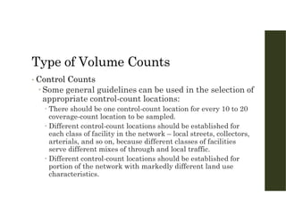
• Control Counts
The hourly and daily variation patters observed at a control
count must be representative of a larger portion of the network
if the sampling procedure is to be accurate and meaningful.
Volume variation patterns are generated by land-use
characteristics and by the type of traffic, particularly the
percentages of through versus locally generated traffic in the
traffic stream
83.
Type of VolumeCounts
• Control Counts
Some general guidelines can be used in the selection of
appropriate control-count locations:
There should be one control-count location for every 10 to 20
coverage-count location to be sampled.
Different control-count locations should be established for
each class of facility in the network – local streets, collectors,
arterials, and so on, because different classes of facilities
serve different mixes of through and local traffic.
Different control-count locations should be established for
portion of the network with markedly different land use
characteristics.
84.
Type of VolumeCounts
• Coverage Counts
All locations at which sample counts will be taken are called
coverage counts
All coverage counts (and control counts as well) in a network
study are taken at midblock locations to avoid the difficulty of
separately recording turning movements.
85.
Example 5
• Thefigure shows one segment of a larger
network that has been identified as having
reasonably uniform traffic patterns in time. The
network segment has seven links, one of which
has been established as a control-count location.
Each of the other six links are coverage-count
locations at which sample counts will be
conducted. The various proposed study
procedures all assume there are only two field
crews or automated counters that can be
employed simultaneously in this segment of the
network. A study procedure is need to find the
volume on each link of the network between 12
noon and 8:00PM on a typical weekday.
86.
Example 5
• Oneof the two available crews or setups would be used to count
Control Location A for the entire eight-hour period of the study.
• The second crew or set-up would be used to count each of
Coverage Locations 1 to 6 for one hour.
87.
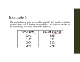
Example 5
• Thecontrol-count data are used to quantify the hourly variation
pattern observed. It is now assumed that this pattern applies to
all of coverage locations within the network.
88.
Example 5
• Thusa count of 840 vehicles at location 1 would represent 0.117 (11.7%) of the eight-hour total
at this location.
• The eight-hour total can then be estimated at 840/0.117 = 7,179 vehicles.
• Moreover, the peak-hour volume can be estimated as 0.163 x 7,179 = 1,170 vehicles because the
hourly distribution shows that the highest volume hour contains 0.163 (or 16.3%) of the eight-
hour volume.
• Note that this expansion of data results in estimates of eight-hour and peak-hour volumes at
each of the seven count locations that represent the day on which the counts were taken.
89.
Example 5
• Hourlyvariation patterns are not as stable as variations for
larger periods of time
• It could be argued that a better approach would be to count each
coverage location for a full eight hours
• Given the limitation to two simultaneous counts due to personnel
and/or equipment, such a study would take place over six days.
• One crew would monitor the control location for the entire period
of the study, and the second would count at one coverage location
for eight hours on each of six days.
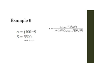
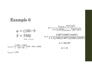
Example 6
• Todetermine a representative value for the ADT on 100 highway
links that have similar volume characteristics, it was decided to
collect 24-hour volume counts on a sample of these links.
Estimates of mean and standard deviation of the link volumes for
the type of highways in which these links are located are 32,500
and 5500, respectively. Determine the minimum number of
stations at which volume counts should be taken if a 95–5
precision level is required with a 10 percent allowable error.
Seatwork
• Assuming areasonably uniform traffic pattern in the transport network
consisting of a series of one-way roads and using the control and coverage
count data summarized in the table below, compute the estimated
morning peak-hour volumes at each of the 5 coverage count locations, as
well as location G.
Coverage
Control A
Time Count
Location
Count
1150
04 - 05
1513
05 - 06
925
B
1662
06 - 07
722
C
1738
07 - 08
511
D
1454
08 - 09
758
E
1257
09 - 10
833
F
1117
10 - 11
1075
11 - 12
B = 962 E = 1041
C = 722 F = 1290
D = 607 G = 1050

![Measures of Effectiveness Defining
Levels of Service in HCM 2000
Measure of Effectiveness
Type of Facility
Type of Flow
Density [pc/mi/ln]
Density [pc/mi/ln]
Density [pc/mi/ln]
Density [pc/mi/ln]
Average Travel Speed [mi/hr]
Percent Time Spent Following [%]
Freeways
Basic sections
Weaving areas
Ramp junctions
Multilane Highways
Two-Lane Highways
Uninterrupted
Flow
Control Delay [s/veh]
Control Delay [s/veh]
Average Travel Speed [mi/hr]
Service Frequency [veh/day]
Service Headway [min]
Passengers/Seat
Space [ft2/ped]
Frequency of (Conflicting) Events [events/hr]
Signalized Intersections
Unsignalized Intersections
Urban Streets
Transit
Pedestrians
Bicycles
Interrupted
Flow](https://image.slidesharecdn.com/cehiwaylecture03-250530172554-ebb9ed85/85/CEHIWAY_Lecture03-for-engineering-courses-2-320.jpg)