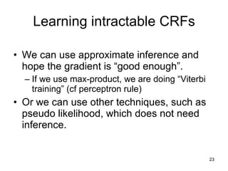
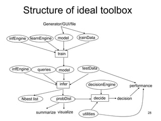
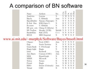
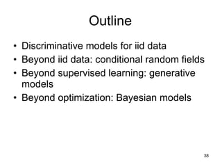
Graphical model software for machine learning Kevin Murphy University of British Columbia   December,  2005
Outline Discriminative models for iid data Beyond iid data: conditional random fields Beyond supervised learning: generative models Beyond optimization: Bayesian models
Supervised learning as Bayesian inference  Y 1 X 1 Y N X N Y * X *  Y n X n Y * X * N Training Testing
Supervised learning as optimization  Y 1 X 1 Y N X N Y * X *  Y n X n Y * X * N Training Testing
Example: logistic regression Let y n   2  {1,…,C} be given by a softmax Maximize conditional log likelihood  “ Max margin” solution
Outline Discriminative models for iid data Beyond iid data: conditional random fields Beyond supervised learning: generative models Beyond optimization: Bayesian models
1D chain CRFs for sequence labeling  Y n1 Y nm Y n2 X n A 1D conditional random field (CRF) is an extension of logistic regression to the case where the output labels are sequences, y n   2  {1,…,C} m   Local evidence Edge potential  i  ij
2D Lattice CRFs for pixel labeling A conditional random field (CRF)  is a discriminative model of P(y|x). The edge potentials  ij  are image dependent.
2D Lattice MRFs for pixel labeling A Markov Random Field (MRF) is an undirected graphical model. Here we model  correlation between pixel labels using   ij (y i ,y j ). We also have a per-pixel generative model of observations P(x i |y i ) Local evidence Potential function Partition function
Tree-structured CRFs Used in parts-based object detection Y i  is location of part i in image eyeL nose eyeR mouth Fischler & Elschlager, "The representation and matching of pictorial structures”, PAMI’73 Felzenszwalb & Huttenlocher, "Pictorial Structures for Object Recognition," IJCV’05
General  CRFs In general, the graph may have arbitrary structure eg for collective web page classification, nodes=urls, edges=hyperlinks The potentials are in general defined on cliques, not just edges
Factor graphs Square nodes = factors (potentials) Round nodes = random variables Graph structure = bipartite
Potential functions For the local evidence, we can use a discriminative classifier (trained iid) For the edge compatibilities, we can use a maxent/ loglinear form, using pre-defined features
Restricted potential functions For some applications (esp in vision), we often use a Potts model of the form We can generalize this for ordered labels (eg discretization of continuous states)   l
 
Learning CRFs If the log likelihood is then the gradient is cliques Gradient = features – expected features Tied params
Learning CRFs Given the gradient  r d , one can find the global optimum using first or second order optimization methods, such as Conjugate gradient Limited memory BFGS Stochastic meta descent (SMD)? The bottleneck is computing the expected features needed for the gradient
Exact inference For 1D chains, one can compute P(y i,i+1 |x) exactly in O(N K 2 ) time using belief propagation (BP = forwards backwards algorithm) For restricted potentials (eg   ij =  (   l)), one can do this in O(NK) time using FFT-like tricks This can be generalized to trees.
Sum-product vs max-product We use sum-product to compute marginal probabilities needed for learning We use max-product to find the most probable assignment (Viterbi decoding) We can also compute max-marginals
Complexity of exact inference In general, the running time is   (N K w ), where w is the treewidth of the graph; this is the size of the maximal clique of the triangulated graph (assuming an optimal elimination ordering). For chains and trees, w = 2. For n  £  n lattices, w = O(n).
Approximate sum-product O(N K I) General Mean field O(N K I) General Swendsen-Wang O(N K I) General Gibbs O(N K 2c  I) c = cluster size General Generalized BP O(N K I) Restricted BP+FFT (exact iff tree) O(N K 2  I) General BP (exact iff tree) Time N=num nodes, K = num states, I = num iterations Potential (pairwise) Algorithm
Approximate max-product O(N K I) General SLS (stochastic local search) O(N K I) General ICM (iterated conditional modes) O(N 2  K I)  [?] Restricted Graph-cuts (exact iff K=2) O(N K 2c  I) c = cluster size General Generalized BP O(N K I) Restricted BP+DT (exact iff tree) O(N K 2  I) General BP (exact iff tree) Time N=num nodes, K = num states, I = num iterations Potential (pairwise) Algorithm
Learning intractable CRFs We can use approximate inference and hope the gradient is “good enough”. If we use max-product, we are doing “Viterbi training” (cf perceptron rule) Or we can use other techniques, such as pseudo likelihood, which does not need inference.
Pseudo-likelihood
Software for inference and learning in 1D CRFs Various packages Mallet (McCallum et al) – Java Crf.sourceforge.net (Sarawagi, Cohen) – Java My code – matlab (just a toy, not integrated with BNT) Ben Taskar says he will soon release his Max Margin Markov net code (which uses LP for inference and QP for learning). Nothing standard, emphasis on NLP apps
Software for inference in general CRFs/ MRFs Max-product : C++ code for GC, BP, TRP and ICM (for Lattice2) by Rick Szeliski et al “ A comparative study of energy minimization methods for MRFs”, Rick Szeliksi, Ramin Zabih, Daniel Scharstein, Olga Veksler, Vladimir Kolmogorov, Aseem Agarwala, Marsall Tappen, Carsten Rother Sum-product for  Gaussian  MRFs: GMRFlib, C code by Havard Rue (exact inference) Sum-product: various other ad hoc pieces My matlab BP code (MRF2) Rivasseau’s C++ code for BP, Gibbs, tree-sampling (factor graphs) Metlzer’s C++ code for BP, GBP, Gibbs, MF (Lattice2)
Software for learning general MRFs/CRFs Hardly any! Parise’s matlab code (approx gradient, pseudo likelihood, CD, etc) My matlab code (IPF, approx gradient – just a toy – not integrated with BNT)
Structure of ideal toolbox train performance visualize summarize Generator/GUI/file infer decisionEngine utilities decision testData trainData learnEngine infEngine queries model model infEngine probDist decide Nbest list
Structure of BNT train visualize summarize Generator/GUI/file infer testData decisionEngine BP Jtree MCMC EM StructuralEM Graphs+CPDs Graphs+CPDs LeRay Shan Cell array NodeIds VarElim N=1 (MAP) Array, Gaussian, samples LIMID Jtree VarElim policy Cell array trainData learnEngine infEngine queries model model infEngine probDist decide Nbest list
Outline Discriminative models for iid data Beyond iid data: conditional random fields Beyond supervised learning: generative models Beyond optimization: Bayesian models
Unsupervised learning: why? Labeling data is time-consuming. Often not clear what label to use. Complex objects often not describable with a single discrete label. Humans learn without labels. Want to discover novel patterns/ structure.
Unsupervised learning: what? Clusters (eg GMM) Low dim manifolds (eg PCA) Graph structure (eg biology, social networks) “ Features” (eg maxent models of language and texture) “ Objects” (eg sprite models in vision)
Unsupervised learning of objects from video Frey and Jojic; Williams and Titsias ; et al
Unsupervised learning: issues Objective function not as obvious as in supervised learning. Usually try to maximize likelihood (measure of data compression). Local minima (non convex objective). Uses inference as subroutine (can be slow – no worse than discriminative learning)
Unsupervised learning: how? Construct a generative model (eg a Bayes net). Perform inference. May have to use approximations such as maximum likelihood and BP. Cannot use max likelihood for model selection…
A comparison of BN software www.ai.mit.edu/~murphyk/Software/Bayes/bnsoft.html
Popular BN software BNT (matlab) Intel’s PNL (C++) Hugin (commercial) Netica (commercial) GMTk (free .exe from Jeff Bilmes)
Outline Discriminative models for iid data Beyond iid data: conditional random fields Beyond supervised learning: generative models Beyond optimization: Bayesian models
Bayesian inference: why? It is optimal. It can easily incorporate prior knowledge (esp. useful for small n, large p problems). It properly reports confidence in output (useful for combining estimates, and for risk-averse applications). It separates models from algorithms.
Bayesian inference: how? Since we want to integrate, we cannot use max-product. Since the unknown parameters are continuous, we cannot use sum-product. But we can use EP (expectation propagation), which is similar to BP. We can also use variational inference. Or MCMC (eg Gibbs sampling).
General purpose Bayesian software BUGS (Gibbs sampling) VIBES (variational message passing) Minka and Winn’s toolbox (infer.net)
Structure of ideal  Bayesian  toolbox train performance visualize summarize Generator/ GUI/ file infer decisionEngine utilities decision testData trainData learnEngine infEngine queries model model infEngine probDist decide

Software tookits for machine learning and graphical models

  • 1.
    Graphical model softwarefor machine learning Kevin Murphy University of British Columbia December, 2005
  • 2.
    Outline Discriminative modelsfor iid data Beyond iid data: conditional random fields Beyond supervised learning: generative models Beyond optimization: Bayesian models
  • 3.
    Supervised learning asBayesian inference  Y 1 X 1 Y N X N Y * X *  Y n X n Y * X * N Training Testing
  • 4.
    Supervised learning asoptimization  Y 1 X 1 Y N X N Y * X *  Y n X n Y * X * N Training Testing
  • 5.
    Example: logistic regressionLet y n 2 {1,…,C} be given by a softmax Maximize conditional log likelihood “ Max margin” solution
  • 6.
    Outline Discriminative modelsfor iid data Beyond iid data: conditional random fields Beyond supervised learning: generative models Beyond optimization: Bayesian models
  • 7.
    1D chain CRFsfor sequence labeling  Y n1 Y nm Y n2 X n A 1D conditional random field (CRF) is an extension of logistic regression to the case where the output labels are sequences, y n 2 {1,…,C} m Local evidence Edge potential  i  ij
  • 8.
    2D Lattice CRFsfor pixel labeling A conditional random field (CRF) is a discriminative model of P(y|x). The edge potentials  ij are image dependent.
  • 9.
    2D Lattice MRFsfor pixel labeling A Markov Random Field (MRF) is an undirected graphical model. Here we model correlation between pixel labels using  ij (y i ,y j ). We also have a per-pixel generative model of observations P(x i |y i ) Local evidence Potential function Partition function
  • 10.
    Tree-structured CRFs Usedin parts-based object detection Y i is location of part i in image eyeL nose eyeR mouth Fischler & Elschlager, "The representation and matching of pictorial structures”, PAMI’73 Felzenszwalb & Huttenlocher, "Pictorial Structures for Object Recognition," IJCV’05
  • 11.
    General CRFsIn general, the graph may have arbitrary structure eg for collective web page classification, nodes=urls, edges=hyperlinks The potentials are in general defined on cliques, not just edges
  • 12.
    Factor graphs Squarenodes = factors (potentials) Round nodes = random variables Graph structure = bipartite
  • 13.
    Potential functions Forthe local evidence, we can use a discriminative classifier (trained iid) For the edge compatibilities, we can use a maxent/ loglinear form, using pre-defined features
  • 14.
    Restricted potential functionsFor some applications (esp in vision), we often use a Potts model of the form We can generalize this for ordered labels (eg discretization of continuous states)   l
  • 15.
  • 16.
    Learning CRFs Ifthe log likelihood is then the gradient is cliques Gradient = features – expected features Tied params
  • 17.
    Learning CRFs Giventhe gradient r d , one can find the global optimum using first or second order optimization methods, such as Conjugate gradient Limited memory BFGS Stochastic meta descent (SMD)? The bottleneck is computing the expected features needed for the gradient
  • 18.
    Exact inference For1D chains, one can compute P(y i,i+1 |x) exactly in O(N K 2 ) time using belief propagation (BP = forwards backwards algorithm) For restricted potentials (eg  ij =  (  l)), one can do this in O(NK) time using FFT-like tricks This can be generalized to trees.
  • 19.
    Sum-product vs max-productWe use sum-product to compute marginal probabilities needed for learning We use max-product to find the most probable assignment (Viterbi decoding) We can also compute max-marginals
  • 20.
    Complexity of exactinference In general, the running time is  (N K w ), where w is the treewidth of the graph; this is the size of the maximal clique of the triangulated graph (assuming an optimal elimination ordering). For chains and trees, w = 2. For n £ n lattices, w = O(n).
  • 21.
    Approximate sum-product O(NK I) General Mean field O(N K I) General Swendsen-Wang O(N K I) General Gibbs O(N K 2c I) c = cluster size General Generalized BP O(N K I) Restricted BP+FFT (exact iff tree) O(N K 2 I) General BP (exact iff tree) Time N=num nodes, K = num states, I = num iterations Potential (pairwise) Algorithm
  • 22.
    Approximate max-product O(NK I) General SLS (stochastic local search) O(N K I) General ICM (iterated conditional modes) O(N 2 K I) [?] Restricted Graph-cuts (exact iff K=2) O(N K 2c I) c = cluster size General Generalized BP O(N K I) Restricted BP+DT (exact iff tree) O(N K 2 I) General BP (exact iff tree) Time N=num nodes, K = num states, I = num iterations Potential (pairwise) Algorithm
  • 23.
    Learning intractable CRFsWe can use approximate inference and hope the gradient is “good enough”. If we use max-product, we are doing “Viterbi training” (cf perceptron rule) Or we can use other techniques, such as pseudo likelihood, which does not need inference.
  • 24.
  • 25.
    Software for inferenceand learning in 1D CRFs Various packages Mallet (McCallum et al) – Java Crf.sourceforge.net (Sarawagi, Cohen) – Java My code – matlab (just a toy, not integrated with BNT) Ben Taskar says he will soon release his Max Margin Markov net code (which uses LP for inference and QP for learning). Nothing standard, emphasis on NLP apps
  • 26.
    Software for inferencein general CRFs/ MRFs Max-product : C++ code for GC, BP, TRP and ICM (for Lattice2) by Rick Szeliski et al “ A comparative study of energy minimization methods for MRFs”, Rick Szeliksi, Ramin Zabih, Daniel Scharstein, Olga Veksler, Vladimir Kolmogorov, Aseem Agarwala, Marsall Tappen, Carsten Rother Sum-product for Gaussian MRFs: GMRFlib, C code by Havard Rue (exact inference) Sum-product: various other ad hoc pieces My matlab BP code (MRF2) Rivasseau’s C++ code for BP, Gibbs, tree-sampling (factor graphs) Metlzer’s C++ code for BP, GBP, Gibbs, MF (Lattice2)
  • 27.
    Software for learninggeneral MRFs/CRFs Hardly any! Parise’s matlab code (approx gradient, pseudo likelihood, CD, etc) My matlab code (IPF, approx gradient – just a toy – not integrated with BNT)
  • 28.
    Structure of idealtoolbox train performance visualize summarize Generator/GUI/file infer decisionEngine utilities decision testData trainData learnEngine infEngine queries model model infEngine probDist decide Nbest list
  • 29.
    Structure of BNTtrain visualize summarize Generator/GUI/file infer testData decisionEngine BP Jtree MCMC EM StructuralEM Graphs+CPDs Graphs+CPDs LeRay Shan Cell array NodeIds VarElim N=1 (MAP) Array, Gaussian, samples LIMID Jtree VarElim policy Cell array trainData learnEngine infEngine queries model model infEngine probDist decide Nbest list
  • 30.
    Outline Discriminative modelsfor iid data Beyond iid data: conditional random fields Beyond supervised learning: generative models Beyond optimization: Bayesian models
  • 31.
    Unsupervised learning: why?Labeling data is time-consuming. Often not clear what label to use. Complex objects often not describable with a single discrete label. Humans learn without labels. Want to discover novel patterns/ structure.
  • 32.
    Unsupervised learning: what?Clusters (eg GMM) Low dim manifolds (eg PCA) Graph structure (eg biology, social networks) “ Features” (eg maxent models of language and texture) “ Objects” (eg sprite models in vision)
  • 33.
    Unsupervised learning ofobjects from video Frey and Jojic; Williams and Titsias ; et al
  • 34.
    Unsupervised learning: issuesObjective function not as obvious as in supervised learning. Usually try to maximize likelihood (measure of data compression). Local minima (non convex objective). Uses inference as subroutine (can be slow – no worse than discriminative learning)
  • 35.
    Unsupervised learning: how?Construct a generative model (eg a Bayes net). Perform inference. May have to use approximations such as maximum likelihood and BP. Cannot use max likelihood for model selection…
  • 36.
    A comparison ofBN software www.ai.mit.edu/~murphyk/Software/Bayes/bnsoft.html
  • 37.
    Popular BN softwareBNT (matlab) Intel’s PNL (C++) Hugin (commercial) Netica (commercial) GMTk (free .exe from Jeff Bilmes)
  • 38.
    Outline Discriminative modelsfor iid data Beyond iid data: conditional random fields Beyond supervised learning: generative models Beyond optimization: Bayesian models
  • 39.
    Bayesian inference: why?It is optimal. It can easily incorporate prior knowledge (esp. useful for small n, large p problems). It properly reports confidence in output (useful for combining estimates, and for risk-averse applications). It separates models from algorithms.
  • 40.
    Bayesian inference: how?Since we want to integrate, we cannot use max-product. Since the unknown parameters are continuous, we cannot use sum-product. But we can use EP (expectation propagation), which is similar to BP. We can also use variational inference. Or MCMC (eg Gibbs sampling).
  • 41.
    General purpose Bayesiansoftware BUGS (Gibbs sampling) VIBES (variational message passing) Minka and Winn’s toolbox (infer.net)
  • 42.
    Structure of ideal Bayesian toolbox train performance visualize summarize Generator/ GUI/ file infer decisionEngine utilities decision testData trainData learnEngine infEngine queries model model infEngine probDist decide