Downloaded 13 times


![Spatio-temporal random fields
! The spatio-temporal graph is
trained to predict each node’s
maximum a posteriori
probability with the marginal
probabilities.
! Generative model predicting
all nodes.
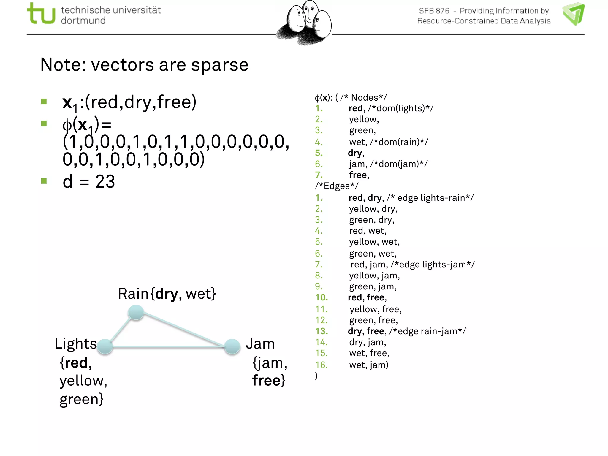
! Dimension
T x |V0| x | X| +
[(T-1)(|V0|+3|E0|)+ |E0|] x |X|2
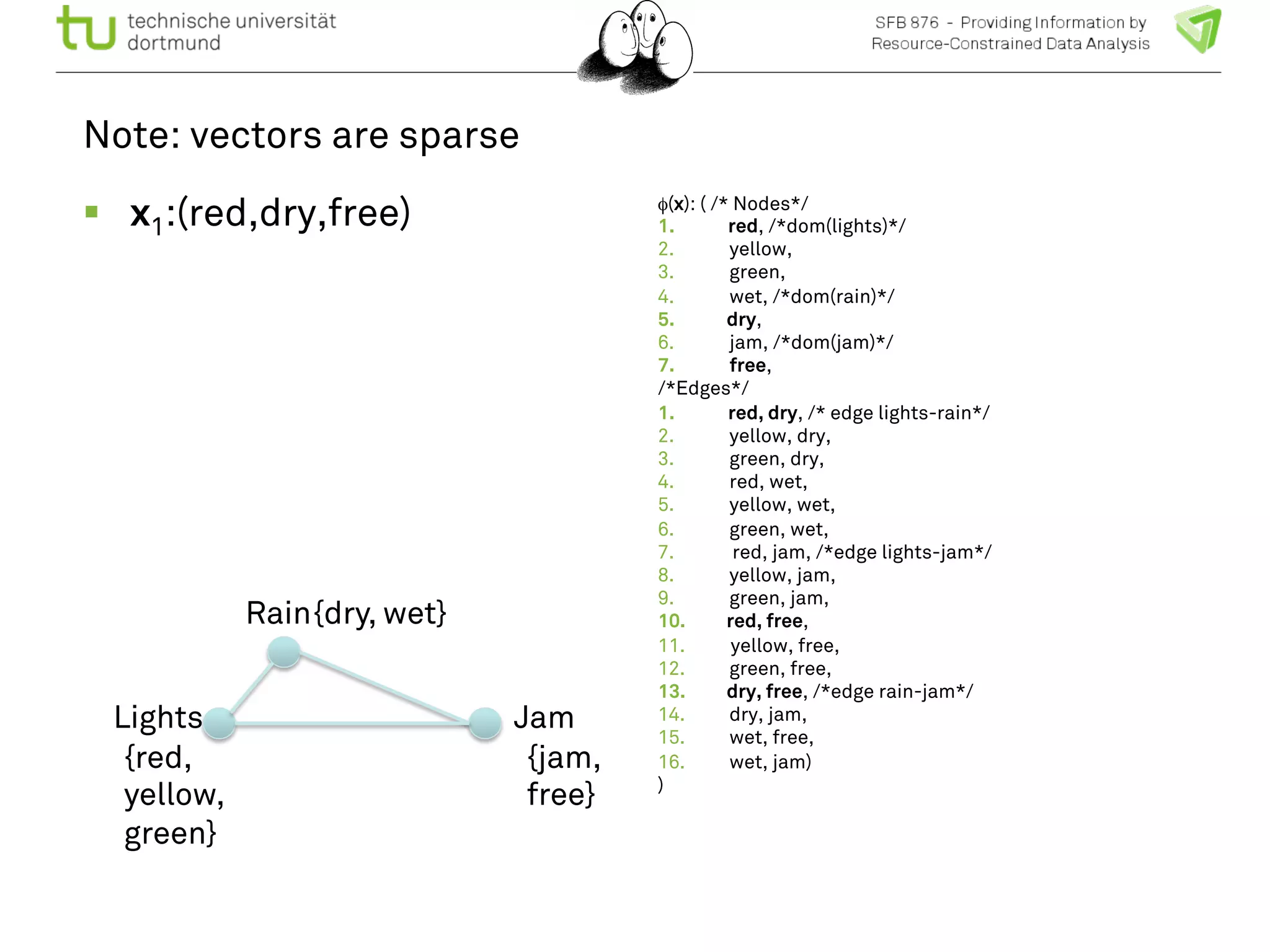
! Remember: vectors are sparse
we have to exploit that!
User queries:
Given traffic densities at all
nodes at t1, t2, t3, what is the
probability of traffic density
at node A at time t5?
Given state “jam” at place A
ts, which other places have a
higher probability for “jam” in
ts < t < te?](https://image.slidesharecdn.com/bigmineinsighttrafficlong-140903002938-phpapp01/75/Big-Data-and-Small-Devices-by-Katharina-Morik-23-2048.jpg)
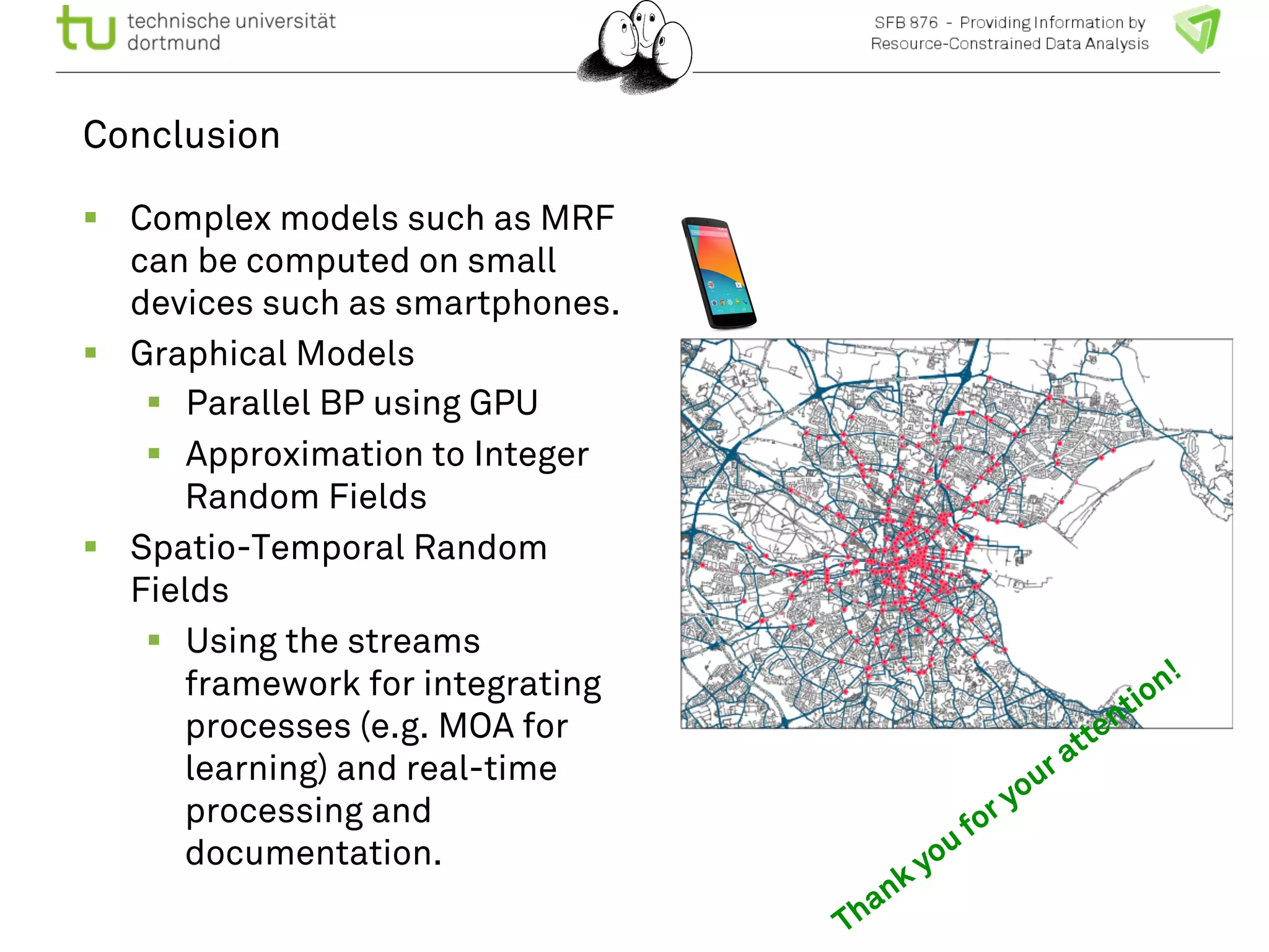

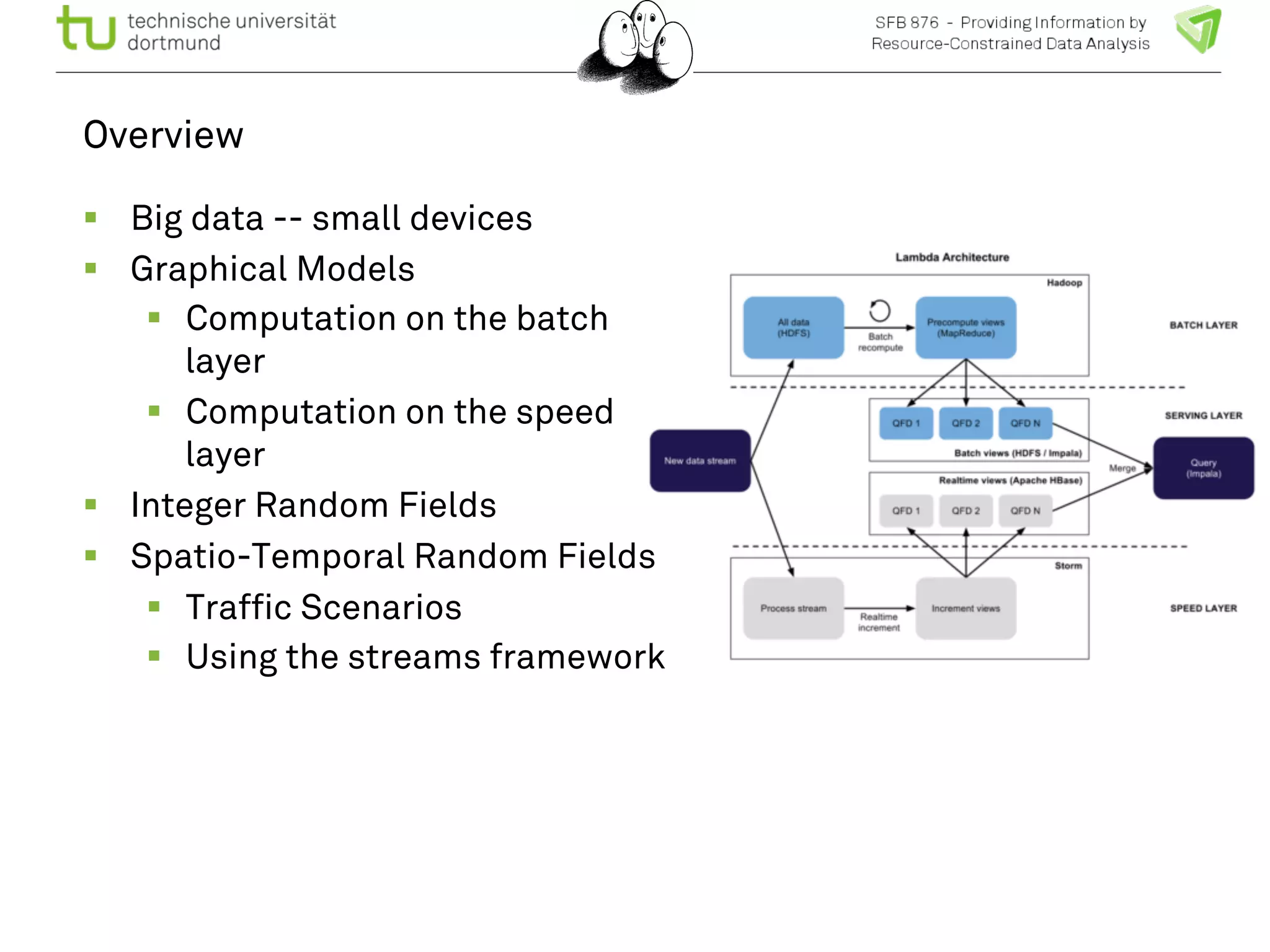
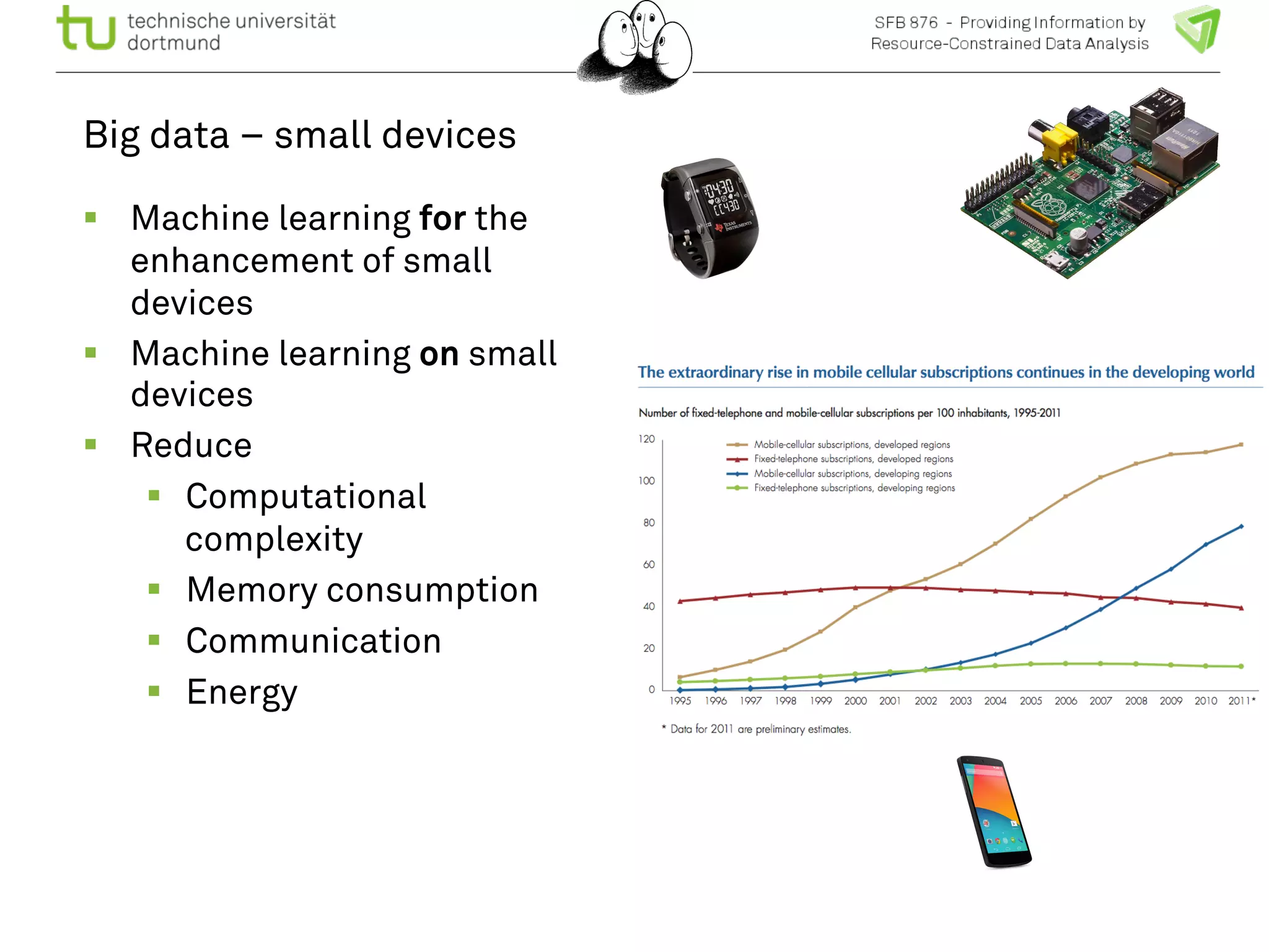
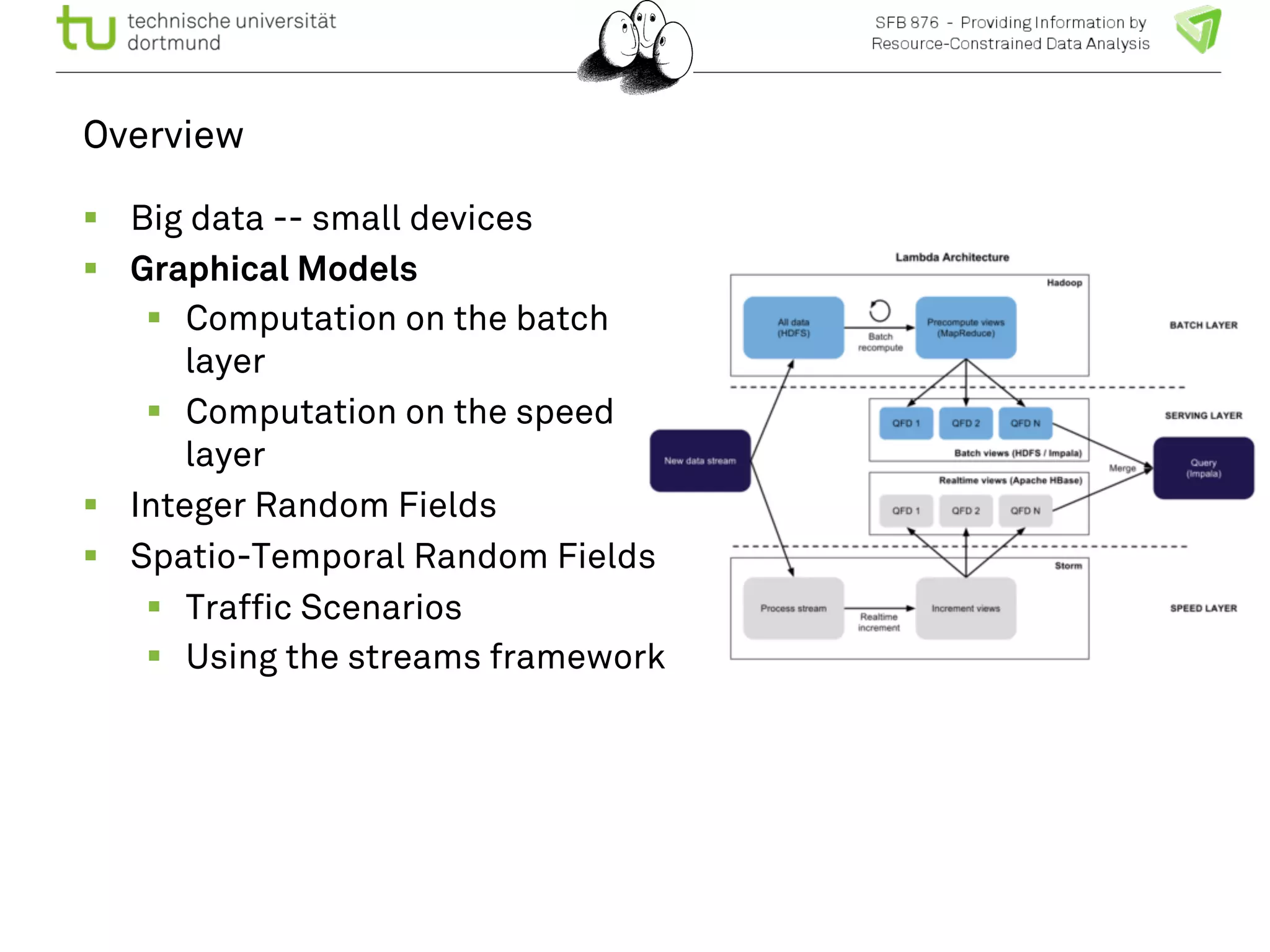
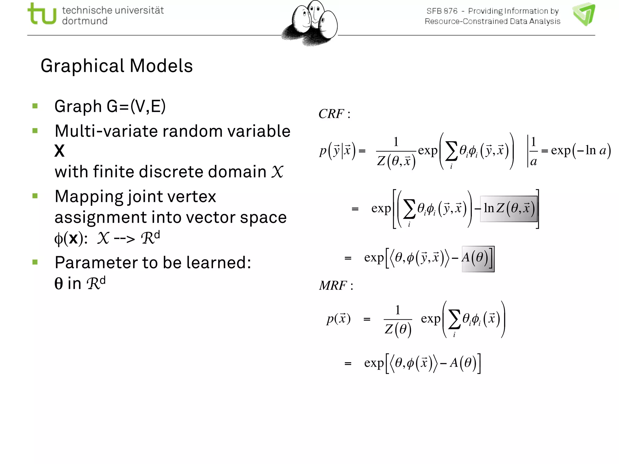
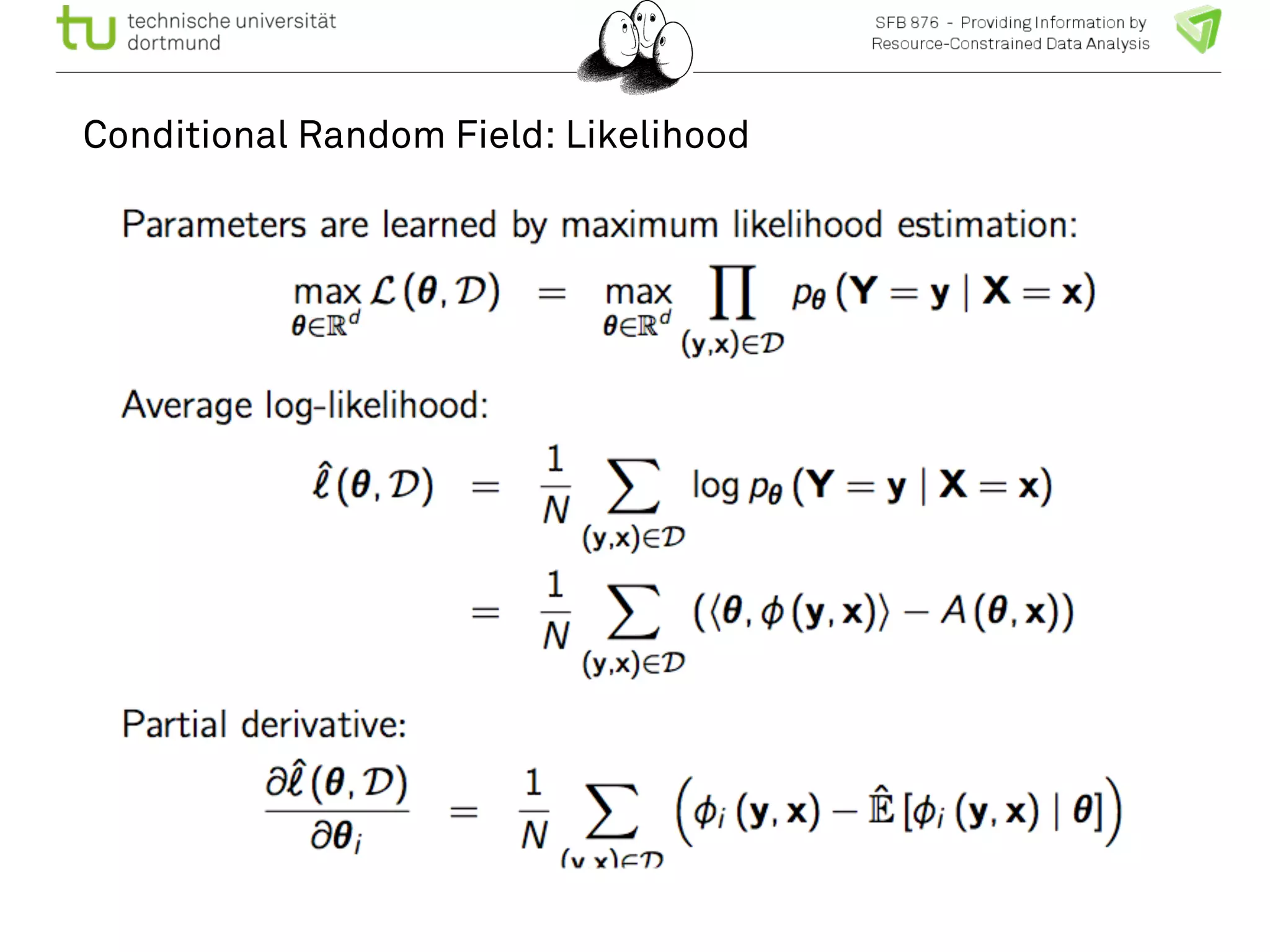
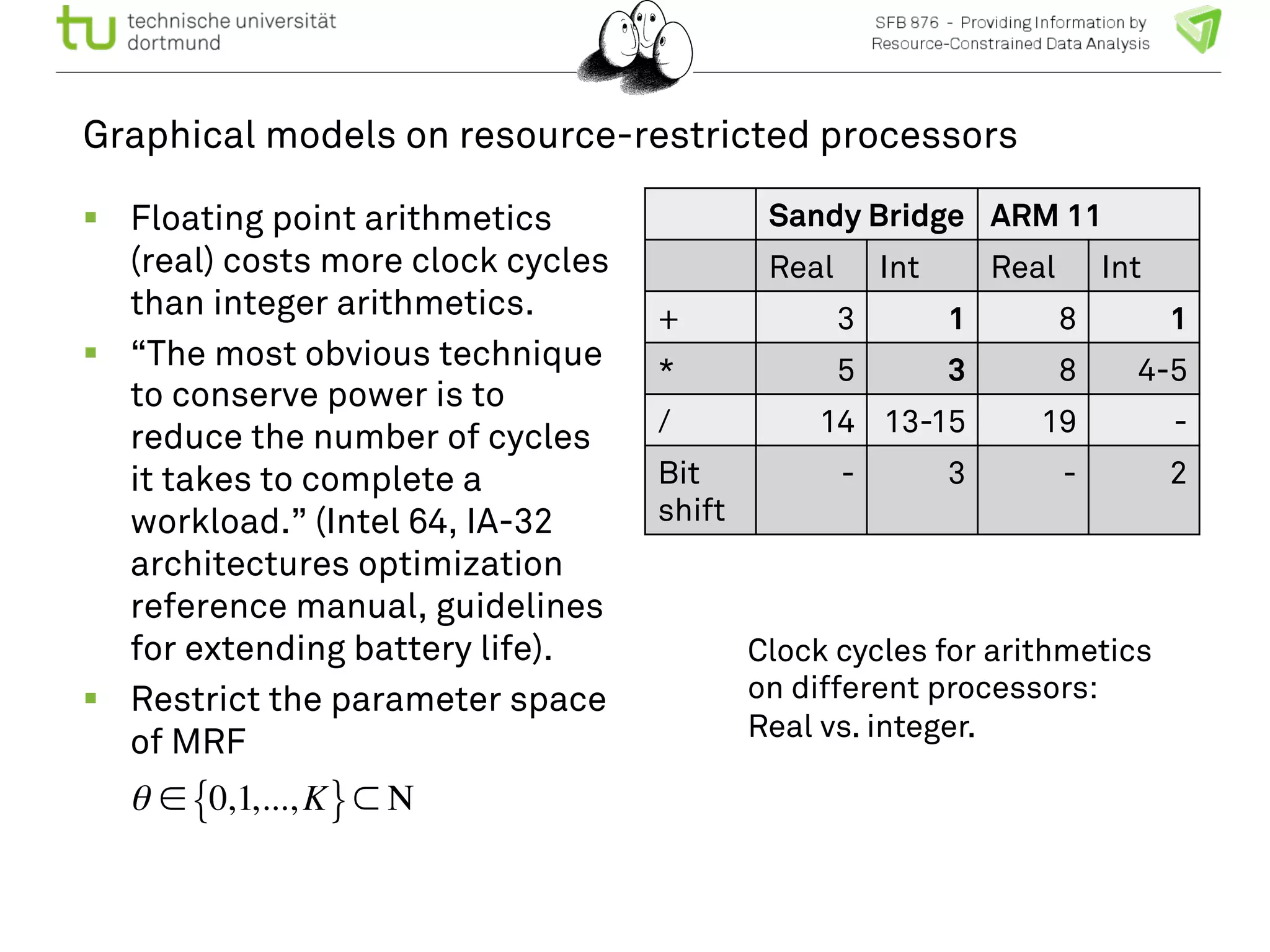
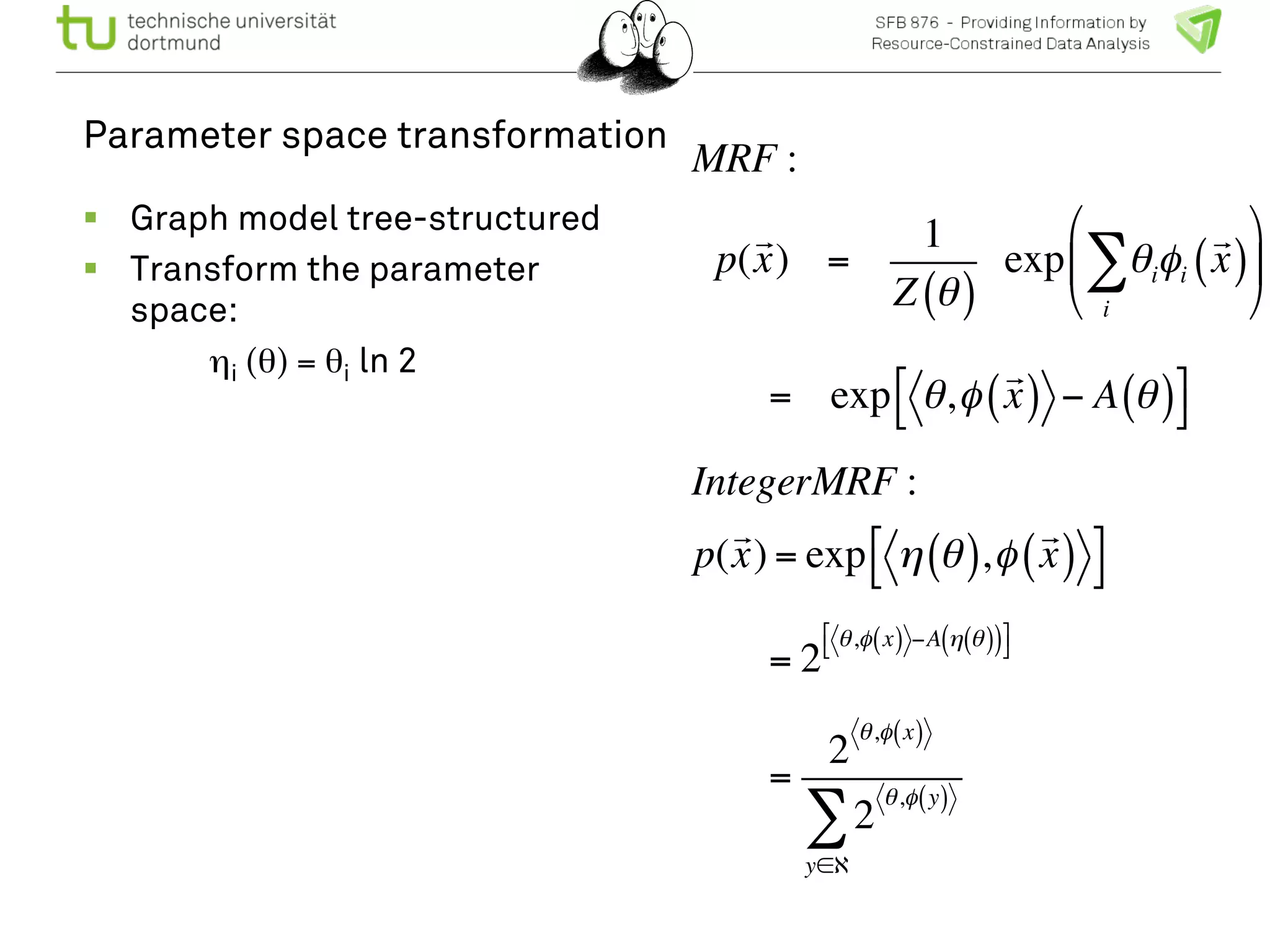
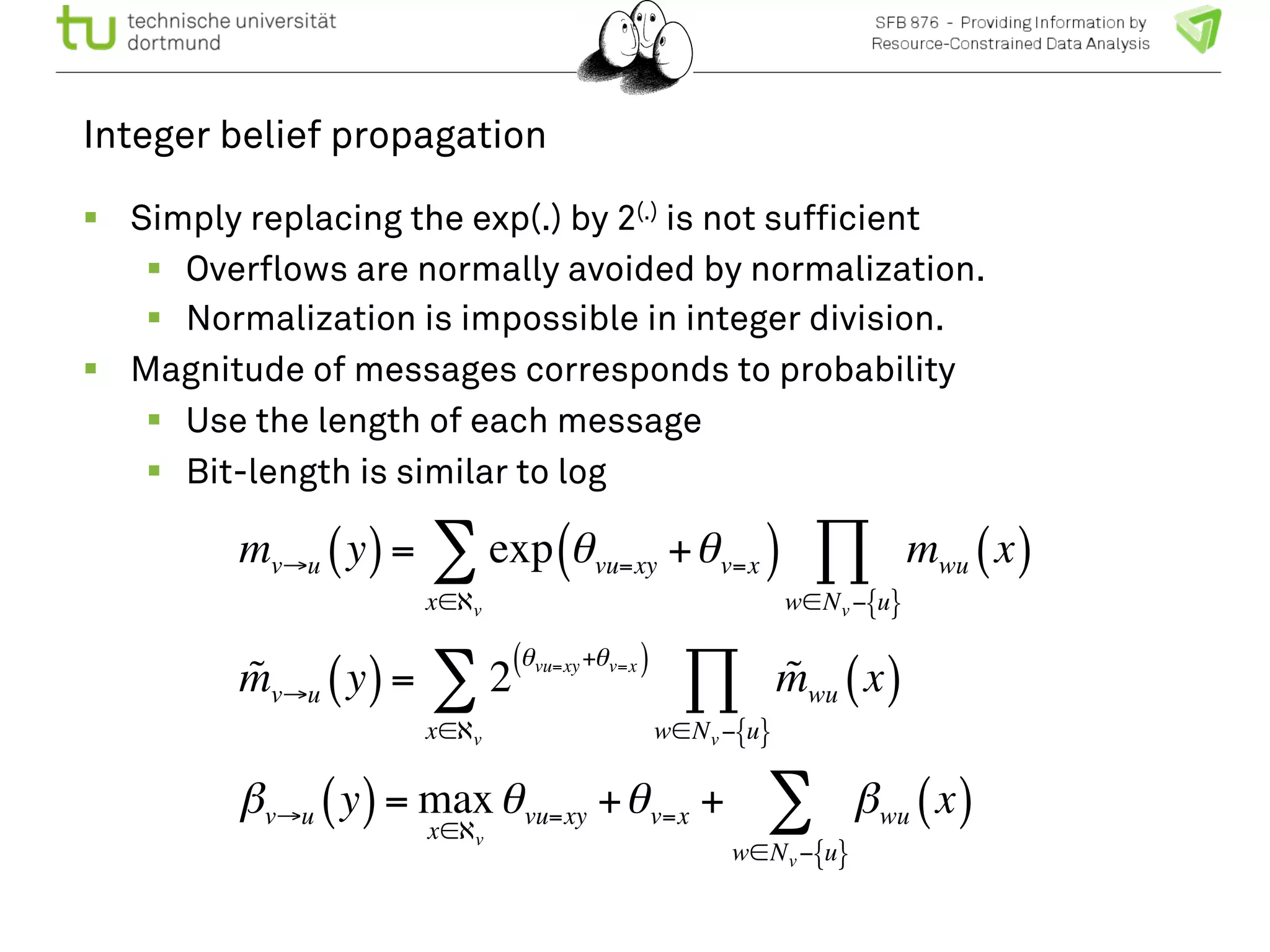
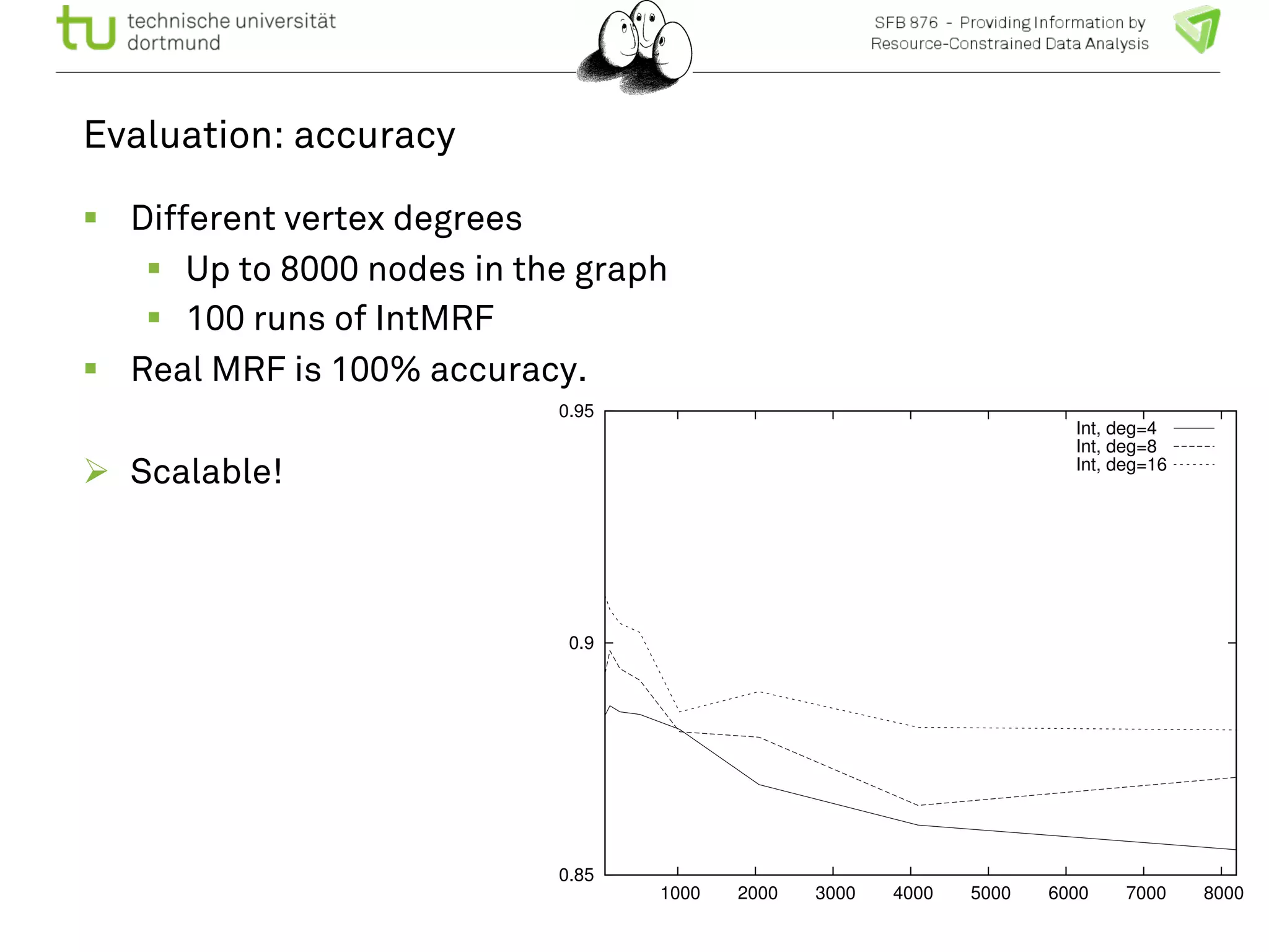
The document discusses the integration of big data and machine learning in enhancing small devices, particularly through the use of graphical models and spatio-temporal random fields for traffic prediction and automation. It highlights techniques for reducing computational complexity, memory consumption, and energy usage while performing probabilistic inference on resource-restricted devices. Additionally, it presents applications in smart traffic management systems and the development of a streaming framework for efficient data processing.