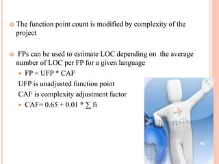
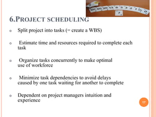
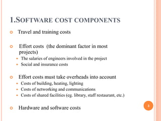
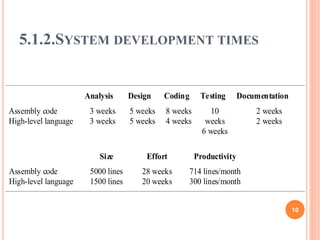
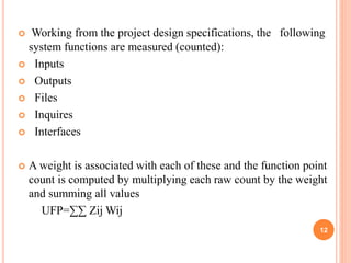
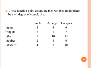
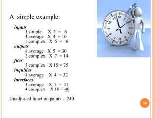
The document discusses software cost estimation and scheduling. It covers topics like software cost components, productivity measures, estimation techniques like function point analysis and lines of code, and project scheduling. Function point analysis measures functionality based on user requirements and design specifications by counting inputs, outputs, files, inquiries and interfaces. Estimates are adjusted based on complexity factors. Estimates are used to determine effort and schedule tasks on a project.

1. SOFTWARE COST AND SCHEDULE
ESTIMATION
Presented By:
Deep kumar sharma
Mtech(1st sem)
1

2. TOPICS COVERED
1. Software Cost components
2. Software productivity
3. Productivity measures
4. Measurement problems
5. Estimation techniques
6. Project scheduling
7. References
2

3. 1.SOFTWARE COST COMPONENTS
 Travel and training costs
 Effort costs (the dominant factor in most
projects)
 The salaries of engineers involved in the project
 Social and insurance costs
 Effort costs must take overheads into account
 Costs of building, heating, lighting
 Costs of networking and communications
 Costs of shared facilities (eg. library, staff restaurant, etc.)
 Hardware and software costs 3

4. 2.SOFTWARE PRODUCTIVITY
 A measure of the rate at which individual engineers
involved in software development produce software and
associated documentation
 Not quality-oriented although quality assurance is a factor
in productivity assessment
 Essentially, we want to measure useful functionality
produced per time unit
4

5. 3.PRODUCTIVITY MEASURES
 Function-related measures based on an estimate of
the functionality of the delivered software. Function-
points are the best known of this type of measure
 Size related measures based on some output from
the software process. This may be lines of delivered
source code, object code instructions, etc
5

6. 4.MEASUREMENT PROBLEMS
 Estimating the size of the measure (e.g. how many function
points)
 Estimating the total number of programmer
months that have elapsed
 Estimating contractor productivity (e.g.
documentation team) and incorporating this
estimate in overall estimate
6

7. 5.ESTIMATION TECHNIQUES
5.1. SOURCE LINES OF CODE
5.2. FUNCTION POINT ANALYSIS
7

8. 5.1.SOURCE LINES OF CODE
 LOC is a software metric used to measure the size of a
computer program by counting the number of lines in the text
of the program's source code
 LOC is typically used to predict the amount of effort that will
be required to develop a program, as well as to estimate
programming productivity or maintainability once the software
is produced
 This model assumes that there is a linear relationship between
system size and volume of documentation
8

9. 5.1.1.PRODUCTIVITY COMPARISONS
 The lower level the language, the more productive the
programmer
 The same functionality takes more code to implement in a lower-
level language than in a high-level language
 The more verbose the programmer, the higher the
productivity
 Measures of productivity based on lines of code suggest that
programmers who write verbose code are more productive than
programmers who write compact code
9

10. 5.1.2.SYSTEM DEVELOPMENT TIMES
Analysis Design Coding Testing Documentation
Assembly code
High-level language
3 weeks
3 weeks
5 weeks
5 weeks
8 weeks
4 weeks
10
weeks
6 weeks
2 weeks
2 weeks
Size Effort Productivity
Assembly code
High-level language
5000 lines
1500 lines
28 weeks
20 weeks
714 lines/month
300 lines/month
10

11. 5.2.FUNCTION POINT ANALYSIS
 Function point metric is that it can be used to easily
estimate the size of a software product directly from the
problem specification
 The idea underlying the FP metric is that the size of a
software product is directly dependent on the no. of
different function or features it support
 The function point analysis measure quantities the
functionality requested and provided to the user based on
the user’s requirements and high level logical design
11

12.  Working from the project design specifications, the following
system functions are measured (counted):
 Inputs
 Outputs
 Files
 Inquires
 Interfaces
 A weight is associated with each of these and the function point
count is computed by multiplying each raw count by the weight
and summing all values
UFP=∑∑ Zij Wij
12

13.  These function-point counts are then weighed (multiplied)
by their degree of complexity:
Simple Average Complex
Inputs 2 4 6
Outputs 3 5 7
Files 5 10 15
Inquires 2 4 6
Interfaces 4 7 10
13

14. A simple example:
inputs
3 simple X 2 = 6
4 average X 4 = 16
1 complex X 6 = 6
outputs
6 average X 5 = 30
2 complex X 7 = 14
files
5 complex X 15 = 75
inquiries
8 average X 4 = 32
interfaces
3 average X 7 = 21
4 complex X 10 = 40
Unadjusted function points - 240
14

15. Adjustment factor
Complex internal processing = 3
Code to be reusable = 2
High performance = 4
Multiple sites = 3
Distributed processing = 5
Project adjustment factor = 17
Adjustment calculation:
Adjusted FP = Unadjusted FP X [0.65 + (adjustment factor X
0.01)]
= 240 X [0.65 + (17 X 0.01)]
= 240 X [0.82]
= 197 Adjusted function points
15

16.  The function point count is modified by complexity of the
project
 FPs can be used to estimate LOC depending on the average
number of LOC per FP for a given language
 FP = UFP * CAF
UFP is unadjusted function point
CAF is complexity adjustment factor
 CAF= 0.65 + 0.01 * ∑ fi
16

17. 6.PROJECT SCHEDULING
 Split project into tasks (= create a WBS)
 Estimate time and resources required to complete each
task
 Organize tasks concurrently to make optimal
use of workforce
 Minimize task dependencies to avoid delays
caused by one task waiting for another to complete
 Dependent on project managers intuition and
experience 17

18.  Once tasks (from the WBS) and size/effort (from
estimation) are known: then schedule
 Primary objectives
• Best time
• Least cost
• Least risk
 Secondary objectives
• Evaluation of schedule alternatives
• Effective use of resources
• Communications
18

19. 8.REFERENCES
 http://www.cfm.va.gov/til/dManual/dmCost.pdf
 http://doit.maryland.gov/SDLC/Documents/Cost_Estimating
.pdf
 http://www.efcog.org/wg/pm_ce/docs/OMBE_Guidelines.
pdf
 http://www.infosys.com/infosys-
labs/publications/Documents/practical-software-
estimation.pdf 19

20. 20