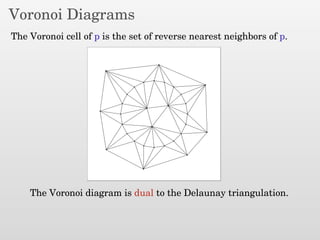
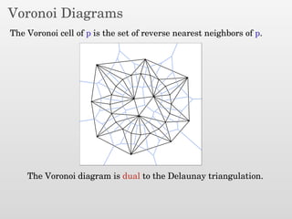
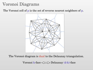
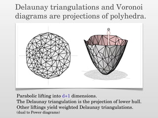
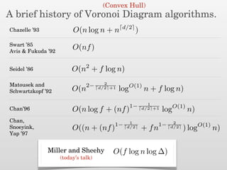
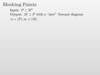
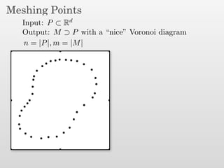
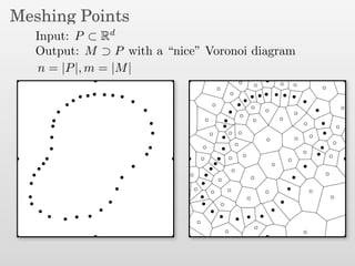
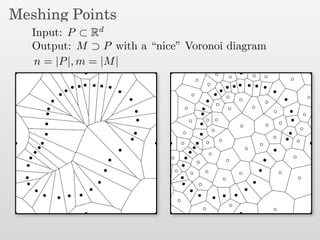
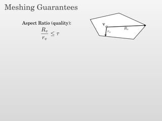
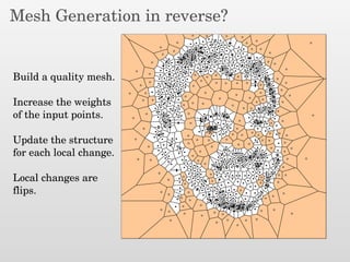
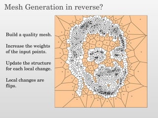
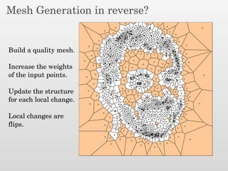
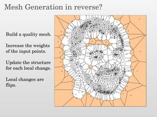
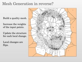
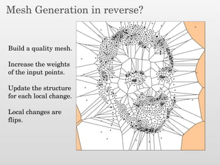
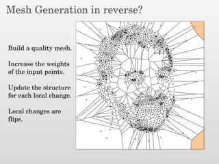
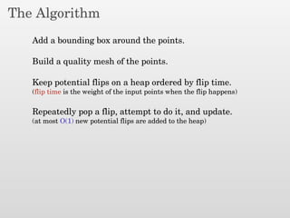
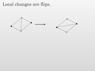
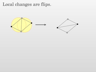
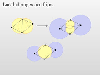
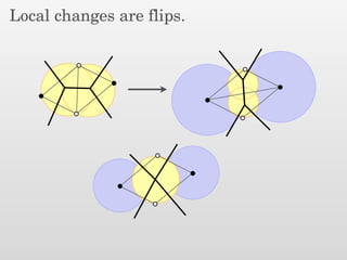
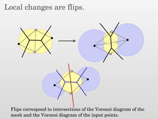
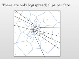
A New Approach to Output-Sensitive
Voronoi Diagrams
and
Delaunay Triangulations
Don Sheehy
INRIA Saclay, France
soon: UConn
Joint work with Gary Miller at CMU
Voronoi Diagrams
Voronoi Diagrams
The Voronoi cell of p is the set of reverse nearest neighbors of p.
Voronoi Diagrams
The Voronoi cell of p is the set of reverse nearest neighbors of p.
Voronoi Diagrams
The Voronoi cell of p is the set of reverse nearest neighbors of p.
The Voronoi diagram is dual to the Delaunay triangulation.
Voronoi Diagrams
The Voronoi cell of p is the set of reverse nearest neighbors of p.
The Voronoi diagram is dual to the Delaunay triangulation.
Voronoi Diagrams
The Voronoi cell of p is the set of reverse nearest neighbors of p.
The Voronoi diagram is dual to the Delaunay triangulation.
Voronoi Diagrams
The Voronoi cell of p is the set of reverse nearest neighbors of p.
The Voronoi diagram is dual to the Delaunay triangulation.
Voronoi k-face Delaunay (d-k)-face
Voronoi Diagrams and Delaunay
triangulations are used everywhere.
Voronoi Diagrams and Delaunay
triangulations are used everywhere.
Geographical Information Systems
Voronoi Diagrams and Delaunay
triangulations are used everywhere.
Geographical Information Systems
Graphics
Voronoi Diagrams and Delaunay
triangulations are used everywhere.
Geographical Information Systems
Graphics
Topological Data Analysis
Voronoi Diagrams and Delaunay
triangulations are used everywhere.
Geographical Information Systems
Graphics
Topological Data Analysis
Mesh Generation
Delaunay triangulations and Voronoi
diagrams are projections of polyhedra.
Delaunay triangulations and Voronoi
diagrams are projections of polyhedra.
Parabolic lifting into d+1 dimensions.
The Delaunay triangulation is the projection of lower hull.
Other liftings yield weighted Delaunay triangulations.
(dual to Power diagrams)
Delaunay triangulations and Voronoi
diagrams are projections of polyhedra.
Parabolic lifting into d+1 dimensions.
The Delaunay triangulation is the projection of lower hull.
Other liftings yield weighted Delaunay triangulations.
(dual to Power diagrams)
Weighted Voronoi Diagrams (aka Power Diagrams)
The diagrams remain piecewise linear.
Weighted Voronoi Diagrams (aka Power Diagrams)
The diagrams remain piecewise linear.
Some points disappear.
Weighted Voronoi Diagrams (aka Power Diagrams)
The diagrams remain piecewise linear.
Some points disappear.
Circumballs are replaced by orthoballs.
Weighted Voronoi Diagrams (aka Power Diagrams)
The diagrams remain piecewise linear.
Some points disappear.
Circumballs are replaced by orthoballs.
A brief history of Voronoi Diagram algorithms.
(Convex Hull)
A brief history of Voronoi Diagram algorithms.
O(n log n + n d/2
)Chazelle ’93
(Convex Hull)
A brief history of Voronoi Diagram algorithms.
O(n log n + n d/2
)Chazelle ’93
(Convex Hull)
Swart ’85
Avis & Fukuda ’92
O(nf)
A brief history of Voronoi Diagram algorithms.
O(n log n + n d/2
)Chazelle ’93
(Convex Hull)
Swart ’85
Avis & Fukuda ’92
O(nf)
O(n2
+ f log n)Seidel ’86
A brief history of Voronoi Diagram algorithms.
O(n log n + n d/2
)Chazelle ’93
(Convex Hull)
Swart ’85
Avis & Fukuda ’92
O(nf)
O(n2
+ f log n)Seidel ’86
O(n2− 2
d/2 +1 logO(1)
n + f log n)
Matousek and
Schwartzkopf ’92
A brief history of Voronoi Diagram algorithms.
O(n log n + n d/2
)Chazelle ’93
(Convex Hull)
Swart ’85
Avis & Fukuda ’92
O(nf)
O(n2
+ f log n)Seidel ’86
O(n2− 2
d/2 +1 logO(1)
n + f log n)
Matousek and
Schwartzkopf ’92
O(n log f + (nf)1− 1
d/2 +1 logO(1)
n)Chan’96
A brief history of Voronoi Diagram algorithms.
O(n log n + n d/2
)Chazelle ’93
(Convex Hull)
Swart ’85
Avis & Fukuda ’92
O(nf)
O(n2
+ f log n)Seidel ’86
O(n2− 2
d/2 +1 logO(1)
n + f log n)
Matousek and
Schwartzkopf ’92
O(n log f + (nf)1− 1
d/2 +1 logO(1)
n)Chan’96
O((n + (nf)1− 1
d/2 + fn1− 2
d/2 ) logO(1)
n)
Chan,
Snoeyink,
Yap ’97
A brief history of Voronoi Diagram algorithms.
O(n log n + n d/2
)Chazelle ’93
O(f log n log ∆)Miller and Sheehy
(today’s talk)
(Convex Hull)
Swart ’85
Avis & Fukuda ’92
O(nf)
O(n2
+ f log n)Seidel ’86
O(n2− 2
d/2 +1 logO(1)
n + f log n)
Matousek and
Schwartzkopf ’92
O(n log f + (nf)1− 1
d/2 +1 logO(1)
n)Chan’96
O((n + (nf)1− 1
d/2 + fn1− 2
d/2 ) logO(1)
n)
Chan,
Snoeyink,
Yap ’97
Meshing Points
Input: P ⊂ Rd
Output: M ⊃ P with a “nice” Voronoi diagram
n = |P|, m = |M|
Meshing Points
Input: P ⊂ Rd
Output: M ⊃ P with a “nice” Voronoi diagram
n = |P|, m = |M|
Meshing Points
Input: P ⊂ Rd
Output: M ⊃ P with a “nice” Voronoi diagram
n = |P|, m = |M|
Meshing Points
Input: P ⊂ Rd
Output: M ⊃ P with a “nice” Voronoi diagram
n = |P|, m = |M|
Meshing Points
Input: P ⊂ Rd
Output: M ⊃ P with a “nice” Voronoi diagram
n = |P|, m = |M|
Counterintuitive Fact about Meshing:
It’s sometimes easier to build the Voronoi/Delaunay
of a superset of the input, than of the input alone.
Meshing Guarantees
Meshing Guarantees
Aspect Ratio (quality): v
Rv
rv
Rv
rv
≤ τ
Meshing Guarantees
Aspect Ratio (quality):
Cell Sizing:
v
Rv
rv
Rv
rv
≤ τ
lfs(x) := d(x, P  {NN(x)})
1
K
lfs(v) ≤ Rv ≤ Klfs(v)
Meshing Guarantees
Aspect Ratio (quality):
Cell Sizing:
Constant Local Complexity:
v
Rv
rv
Rv
rv
≤ τ
lfs(x) := d(x, P  {NN(x)})
Each cell has at most a constant number of faces.
1
K
lfs(v) ≤ Rv ≤ Klfs(v)
Meshing Guarantees
Aspect Ratio (quality):
Cell Sizing:
Constant Local Complexity:
Optimal Size:
v
Rv
rv
Rv
rv
≤ τ
lfs(x) := d(x, P  {NN(x)})
|M| = Θ(|Optimal|)
Each cell has at most a constant number of faces.
1
K
lfs(v) ≤ Rv ≤ Klfs(v)
Meshing Guarantees
Aspect Ratio (quality):
Cell Sizing:
Constant Local Complexity:
Optimal Size:
v
Rv
rv
Rv
rv
≤ τ
lfs(x) := d(x, P  {NN(x)})
|M| = Θ(|Optimal|)
Running time: O(n log n + |M|)
Each cell has at most a constant number of faces.
1
K
lfs(v) ≤ Rv ≤ Klfs(v)
Mesh Generation in reverse?
Build a quality mesh.
Mesh Generation in reverse?
Build a quality mesh.
Increase the weights
of the input points.
Mesh Generation in reverse?
Build a quality mesh.
Increase the weights
of the input points.
Update the structure
for each local change.
Mesh Generation in reverse?
Build a quality mesh.
Increase the weights
of the input points.
Update the structure
for each local change.
Local changes are
flips.
Mesh Generation in reverse?
Build a quality mesh.
Increase the weights
of the input points.
Update the structure
for each local change.
Local changes are
flips.
Mesh Generation in reverse?
Build a quality mesh.
Increase the weights
of the input points.
Update the structure
for each local change.
Local changes are
flips.
Mesh Generation in reverse?
Build a quality mesh.
Increase the weights
of the input points.
Update the structure
for each local change.
Local changes are
flips.
Mesh Generation in reverse?
Build a quality mesh.
Increase the weights
of the input points.
Update the structure
for each local change.
Local changes are
flips.
Mesh Generation in reverse?
Build a quality mesh.
Increase the weights
of the input points.
Update the structure
for each local change.
Local changes are
flips.
Mesh Generation in reverse?
Build a quality mesh.
Increase the weights
of the input points.
Update the structure
for each local change.
Local changes are
flips.
Mesh Generation in reverse?
Build a quality mesh.
Increase the weights
of the input points.
Update the structure
for each local change.
Local changes are
flips.
Mesh Generation in reverse?
Build a quality mesh.
Increase the weights
of the input points.
Update the structure
for each local change.
Local changes are
flips.
Mesh Generation in reverse?
Build a quality mesh.
Increase the weights
of the input points.
Update the structure
for each local change.
Local changes are
flips.
Mesh Generation in reverse?
Build a quality mesh.
Increase the weights
of the input points.
Update the structure
for each local change.
Local changes are
flips.
The Algorithm
The Algorithm
Add a bounding box around the points.
The Algorithm
Add a bounding box around the points.
Build a quality mesh of the points.
The Algorithm
Add a bounding box around the points.
Build a quality mesh of the points.
Keep potential flips on a heap ordered by flip time.
The Algorithm
Add a bounding box around the points.
Build a quality mesh of the points.
Keep potential flips on a heap ordered by flip time.
(flip time is the weight of the input points when the flip happens)
The Algorithm
Add a bounding box around the points.
Build a quality mesh of the points.
Keep potential flips on a heap ordered by flip time.
(flip time is the weight of the input points when the flip happens)
Repeatedly pop a flip, attempt to do it, and update.
The Algorithm
Add a bounding box around the points.
Build a quality mesh of the points.
Keep potential flips on a heap ordered by flip time.
(flip time is the weight of the input points when the flip happens)
Repeatedly pop a flip, attempt to do it, and update.
(at most O(1) new potential flips are added to the heap)
When the heap is empty, remove the bounding box and
all incident Delaunay faces.
Local changes are flips.
Flips correspond to intersections of the Voronoi diagram of the
mesh and the Voronoi diagram of the input points.
There are only log(spread) flips per face.
A summary of the analysis.
Full dimensional mesh cells intersect output faces at
most log(spread) times.
A summary of the analysis.
Full dimensional mesh cells intersect output faces at
most log(spread) times.
Since each mesh cell has only a constant number of
faces, we only get O(f log(spread)) total flips.
A summary of the analysis.
Full dimensional mesh cells intersect output faces at
most log(spread) times.
Since each mesh cell has only a constant number of
faces, we only get O(f log(spread)) total flips.
Each flip generates at most O(1) new flips on the heap.
A summary of the analysis.
Full dimensional mesh cells intersect output faces at
most log(spread) times.
Since each mesh cell has only a constant number of
faces, we only get O(f log(spread)) total flips.
Each flip generates at most O(1) new flips on the heap.
The heap operations require O(log n) time each.
Total running time is O(f log n log (spread)).
Summary
Summary
A new output-sensitive algorithm for Voronoi diagrams and
Delaunay triangulations in d-dimensions.
Summary
A new output-sensitive algorithm for Voronoi diagrams and
Delaunay triangulations in d-dimensions.
Start with a quality mesh and then remove the Steiner points.
Summary
A new output-sensitive algorithm for Voronoi diagrams and
Delaunay triangulations in d-dimensions.
Start with a quality mesh and then remove the Steiner points.
Use geometry to bound the combinatorial changes.
Summary
A new output-sensitive algorithm for Voronoi diagrams and
Delaunay triangulations in d-dimensions.
Start with a quality mesh and then remove the Steiner points.
Use geometry to bound the combinatorial changes.
O(f log n log ∆)Running time:
Summary
A new output-sensitive algorithm for Voronoi diagrams and
Delaunay triangulations in d-dimensions.
Start with a quality mesh and then remove the Steiner points.
Use geometry to bound the combinatorial changes.
O(f log n log ∆)Running time:
Thank you.
A New Approach to Output-Sensitive Voronoi Diagrams and Delaunay Triangulations

A New Approach to Output-Sensitive Voronoi Diagrams and Delaunay Triangulations

  • 1.
    A New Approachto Output-Sensitive Voronoi Diagrams and Delaunay Triangulations Don Sheehy INRIA Saclay, France soon: UConn Joint work with Gary Miller at CMU
  • 2.
  • 3.
    Voronoi Diagrams The Voronoicell of p is the set of reverse nearest neighbors of p.
  • 4.
    Voronoi Diagrams The Voronoicell of p is the set of reverse nearest neighbors of p.
  • 5.
    Voronoi Diagrams The Voronoicell of p is the set of reverse nearest neighbors of p. The Voronoi diagram is dual to the Delaunay triangulation.
  • 6.
    Voronoi Diagrams The Voronoicell of p is the set of reverse nearest neighbors of p. The Voronoi diagram is dual to the Delaunay triangulation.
  • 7.
    Voronoi Diagrams The Voronoicell of p is the set of reverse nearest neighbors of p. The Voronoi diagram is dual to the Delaunay triangulation.
  • 8.
    Voronoi Diagrams The Voronoicell of p is the set of reverse nearest neighbors of p. The Voronoi diagram is dual to the Delaunay triangulation. Voronoi k-face Delaunay (d-k)-face
  • 9.
    Voronoi Diagrams andDelaunay triangulations are used everywhere.
  • 10.
    Voronoi Diagrams andDelaunay triangulations are used everywhere. Geographical Information Systems
  • 11.
    Voronoi Diagrams andDelaunay triangulations are used everywhere. Geographical Information Systems Graphics
  • 12.
    Voronoi Diagrams andDelaunay triangulations are used everywhere. Geographical Information Systems Graphics Topological Data Analysis
  • 13.
    Voronoi Diagrams andDelaunay triangulations are used everywhere. Geographical Information Systems Graphics Topological Data Analysis Mesh Generation
  • 14.
    Delaunay triangulations andVoronoi diagrams are projections of polyhedra.
  • 15.
    Delaunay triangulations andVoronoi diagrams are projections of polyhedra. Parabolic lifting into d+1 dimensions. The Delaunay triangulation is the projection of lower hull. Other liftings yield weighted Delaunay triangulations. (dual to Power diagrams)
  • 16.
    Delaunay triangulations andVoronoi diagrams are projections of polyhedra. Parabolic lifting into d+1 dimensions. The Delaunay triangulation is the projection of lower hull. Other liftings yield weighted Delaunay triangulations. (dual to Power diagrams)
  • 17.
    Weighted Voronoi Diagrams(aka Power Diagrams)
  • 18.
    Weighted Voronoi Diagrams(aka Power Diagrams) The diagrams remain piecewise linear.
  • 19.
    Weighted Voronoi Diagrams(aka Power Diagrams) The diagrams remain piecewise linear. Some points disappear.
  • 20.
    Weighted Voronoi Diagrams(aka Power Diagrams) The diagrams remain piecewise linear. Some points disappear. Circumballs are replaced by orthoballs.
  • 21.
    Weighted Voronoi Diagrams(aka Power Diagrams) The diagrams remain piecewise linear. Some points disappear. Circumballs are replaced by orthoballs.
  • 22.
    A brief historyof Voronoi Diagram algorithms. (Convex Hull)
  • 23.
    A brief historyof Voronoi Diagram algorithms. O(n log n + n d/2 )Chazelle ’93 (Convex Hull)
  • 24.
    A brief historyof Voronoi Diagram algorithms. O(n log n + n d/2 )Chazelle ’93 (Convex Hull) Swart ’85 Avis & Fukuda ’92 O(nf)
  • 25.
    A brief historyof Voronoi Diagram algorithms. O(n log n + n d/2 )Chazelle ’93 (Convex Hull) Swart ’85 Avis & Fukuda ’92 O(nf) O(n2 + f log n)Seidel ’86
  • 26.
    A brief historyof Voronoi Diagram algorithms. O(n log n + n d/2 )Chazelle ’93 (Convex Hull) Swart ’85 Avis & Fukuda ’92 O(nf) O(n2 + f log n)Seidel ’86 O(n2− 2 d/2 +1 logO(1) n + f log n) Matousek and Schwartzkopf ’92
  • 27.
    A brief historyof Voronoi Diagram algorithms. O(n log n + n d/2 )Chazelle ’93 (Convex Hull) Swart ’85 Avis & Fukuda ’92 O(nf) O(n2 + f log n)Seidel ’86 O(n2− 2 d/2 +1 logO(1) n + f log n) Matousek and Schwartzkopf ’92 O(n log f + (nf)1− 1 d/2 +1 logO(1) n)Chan’96
  • 28.
    A brief historyof Voronoi Diagram algorithms. O(n log n + n d/2 )Chazelle ’93 (Convex Hull) Swart ’85 Avis & Fukuda ’92 O(nf) O(n2 + f log n)Seidel ’86 O(n2− 2 d/2 +1 logO(1) n + f log n) Matousek and Schwartzkopf ’92 O(n log f + (nf)1− 1 d/2 +1 logO(1) n)Chan’96 O((n + (nf)1− 1 d/2 + fn1− 2 d/2 ) logO(1) n) Chan, Snoeyink, Yap ’97
  • 29.
    A brief historyof Voronoi Diagram algorithms. O(n log n + n d/2 )Chazelle ’93 O(f log n log ∆)Miller and Sheehy (today’s talk) (Convex Hull) Swart ’85 Avis & Fukuda ’92 O(nf) O(n2 + f log n)Seidel ’86 O(n2− 2 d/2 +1 logO(1) n + f log n) Matousek and Schwartzkopf ’92 O(n log f + (nf)1− 1 d/2 +1 logO(1) n)Chan’96 O((n + (nf)1− 1 d/2 + fn1− 2 d/2 ) logO(1) n) Chan, Snoeyink, Yap ’97
  • 30.
    Meshing Points Input: P⊂ Rd Output: M ⊃ P with a “nice” Voronoi diagram n = |P|, m = |M|
  • 31.
    Meshing Points Input: P⊂ Rd Output: M ⊃ P with a “nice” Voronoi diagram n = |P|, m = |M|
  • 32.
    Meshing Points Input: P⊂ Rd Output: M ⊃ P with a “nice” Voronoi diagram n = |P|, m = |M|
  • 33.
    Meshing Points Input: P⊂ Rd Output: M ⊃ P with a “nice” Voronoi diagram n = |P|, m = |M|
  • 34.
    Meshing Points Input: P⊂ Rd Output: M ⊃ P with a “nice” Voronoi diagram n = |P|, m = |M| Counterintuitive Fact about Meshing: It’s sometimes easier to build the Voronoi/Delaunay of a superset of the input, than of the input alone.
  • 35.
  • 36.
    Meshing Guarantees Aspect Ratio(quality): v Rv rv Rv rv ≤ τ
  • 37.
    Meshing Guarantees Aspect Ratio(quality): Cell Sizing: v Rv rv Rv rv ≤ τ lfs(x) := d(x, P {NN(x)}) 1 K lfs(v) ≤ Rv ≤ Klfs(v)
  • 38.
    Meshing Guarantees Aspect Ratio(quality): Cell Sizing: Constant Local Complexity: v Rv rv Rv rv ≤ τ lfs(x) := d(x, P {NN(x)}) Each cell has at most a constant number of faces. 1 K lfs(v) ≤ Rv ≤ Klfs(v)
  • 39.
    Meshing Guarantees Aspect Ratio(quality): Cell Sizing: Constant Local Complexity: Optimal Size: v Rv rv Rv rv ≤ τ lfs(x) := d(x, P {NN(x)}) |M| = Θ(|Optimal|) Each cell has at most a constant number of faces. 1 K lfs(v) ≤ Rv ≤ Klfs(v)
  • 40.
    Meshing Guarantees Aspect Ratio(quality): Cell Sizing: Constant Local Complexity: Optimal Size: v Rv rv Rv rv ≤ τ lfs(x) := d(x, P {NN(x)}) |M| = Θ(|Optimal|) Running time: O(n log n + |M|) Each cell has at most a constant number of faces. 1 K lfs(v) ≤ Rv ≤ Klfs(v)
  • 41.
  • 42.
    Mesh Generation inreverse? Build a quality mesh.
  • 43.
    Mesh Generation inreverse? Build a quality mesh. Increase the weights of the input points.
  • 44.
    Mesh Generation inreverse? Build a quality mesh. Increase the weights of the input points. Update the structure for each local change.
  • 45.
    Mesh Generation inreverse? Build a quality mesh. Increase the weights of the input points. Update the structure for each local change. Local changes are flips.
  • 46.
    Mesh Generation inreverse? Build a quality mesh. Increase the weights of the input points. Update the structure for each local change. Local changes are flips.
  • 47.
    Mesh Generation inreverse? Build a quality mesh. Increase the weights of the input points. Update the structure for each local change. Local changes are flips.
  • 48.
    Mesh Generation inreverse? Build a quality mesh. Increase the weights of the input points. Update the structure for each local change. Local changes are flips.
  • 49.
    Mesh Generation inreverse? Build a quality mesh. Increase the weights of the input points. Update the structure for each local change. Local changes are flips.
  • 50.
    Mesh Generation inreverse? Build a quality mesh. Increase the weights of the input points. Update the structure for each local change. Local changes are flips.
  • 51.
    Mesh Generation inreverse? Build a quality mesh. Increase the weights of the input points. Update the structure for each local change. Local changes are flips.
  • 52.
    Mesh Generation inreverse? Build a quality mesh. Increase the weights of the input points. Update the structure for each local change. Local changes are flips.
  • 53.
    Mesh Generation inreverse? Build a quality mesh. Increase the weights of the input points. Update the structure for each local change. Local changes are flips.
  • 54.
    Mesh Generation inreverse? Build a quality mesh. Increase the weights of the input points. Update the structure for each local change. Local changes are flips.
  • 55.
    Mesh Generation inreverse? Build a quality mesh. Increase the weights of the input points. Update the structure for each local change. Local changes are flips.
  • 56.
  • 57.
    The Algorithm Add abounding box around the points.
  • 58.
    The Algorithm Add abounding box around the points. Build a quality mesh of the points.
  • 59.
    The Algorithm Add abounding box around the points. Build a quality mesh of the points. Keep potential flips on a heap ordered by flip time.
  • 60.
    The Algorithm Add abounding box around the points. Build a quality mesh of the points. Keep potential flips on a heap ordered by flip time. (flip time is the weight of the input points when the flip happens)
  • 61.
    The Algorithm Add abounding box around the points. Build a quality mesh of the points. Keep potential flips on a heap ordered by flip time. (flip time is the weight of the input points when the flip happens) Repeatedly pop a flip, attempt to do it, and update.
  • 62.
    The Algorithm Add abounding box around the points. Build a quality mesh of the points. Keep potential flips on a heap ordered by flip time. (flip time is the weight of the input points when the flip happens) Repeatedly pop a flip, attempt to do it, and update. (at most O(1) new potential flips are added to the heap)
  • 63.
    The Algorithm Add abounding box around the points. Build a quality mesh of the points. Keep potential flips on a heap ordered by flip time. (flip time is the weight of the input points when the flip happens) Repeatedly pop a flip, attempt to do it, and update. (at most O(1) new potential flips are added to the heap) When the heap is empty, remove the bounding box and all incident Delaunay faces.
  • 64.
  • 65.
  • 66.
  • 67.
  • 68.
  • 69.
  • 70.
  • 71.
    Local changes areflips. Flips correspond to intersections of the Voronoi diagram of the mesh and the Voronoi diagram of the input points.
  • 72.
    There are onlylog(spread) flips per face.
  • 73.
    There are onlylog(spread) flips per face.
  • 74.
    There are onlylog(spread) flips per face.
  • 75.
    A summary ofthe analysis.
  • 76.
    A summary ofthe analysis. Full dimensional mesh cells intersect output faces at most log(spread) times.
  • 77.
    A summary ofthe analysis. Full dimensional mesh cells intersect output faces at most log(spread) times. Since each mesh cell has only a constant number of faces, we only get O(f log(spread)) total flips.
  • 78.
    A summary ofthe analysis. Full dimensional mesh cells intersect output faces at most log(spread) times. Since each mesh cell has only a constant number of faces, we only get O(f log(spread)) total flips. Each flip generates at most O(1) new flips on the heap.
  • 79.
    A summary ofthe analysis. Full dimensional mesh cells intersect output faces at most log(spread) times. Since each mesh cell has only a constant number of faces, we only get O(f log(spread)) total flips. Each flip generates at most O(1) new flips on the heap. The heap operations require O(log n) time each.
  • 80.
    A summary ofthe analysis. Full dimensional mesh cells intersect output faces at most log(spread) times. Since each mesh cell has only a constant number of faces, we only get O(f log(spread)) total flips. Each flip generates at most O(1) new flips on the heap. The heap operations require O(log n) time each. Total running time is O(f log n log (spread)).
  • 81.
  • 82.
    Summary A new output-sensitivealgorithm for Voronoi diagrams and Delaunay triangulations in d-dimensions.
  • 83.
    Summary A new output-sensitivealgorithm for Voronoi diagrams and Delaunay triangulations in d-dimensions. Start with a quality mesh and then remove the Steiner points.
  • 84.
    Summary A new output-sensitivealgorithm for Voronoi diagrams and Delaunay triangulations in d-dimensions. Start with a quality mesh and then remove the Steiner points. Use geometry to bound the combinatorial changes.
  • 85.
    Summary A new output-sensitivealgorithm for Voronoi diagrams and Delaunay triangulations in d-dimensions. Start with a quality mesh and then remove the Steiner points. Use geometry to bound the combinatorial changes. O(f log n log ∆)Running time:
  • 86.
    Summary A new output-sensitivealgorithm for Voronoi diagrams and Delaunay triangulations in d-dimensions. Start with a quality mesh and then remove the Steiner points. Use geometry to bound the combinatorial changes. O(f log n log ∆)Running time: Thank you.