Download to read offline
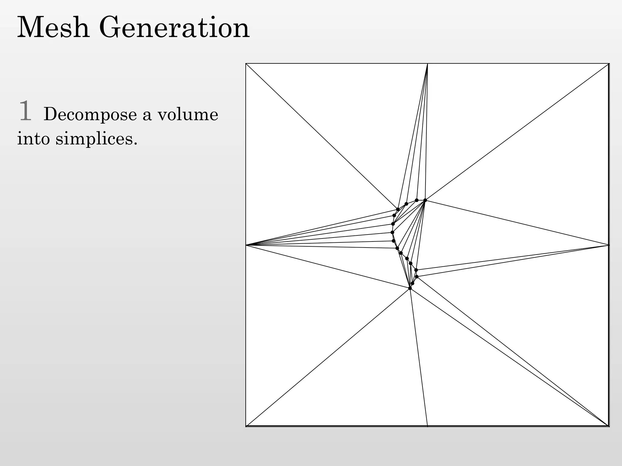
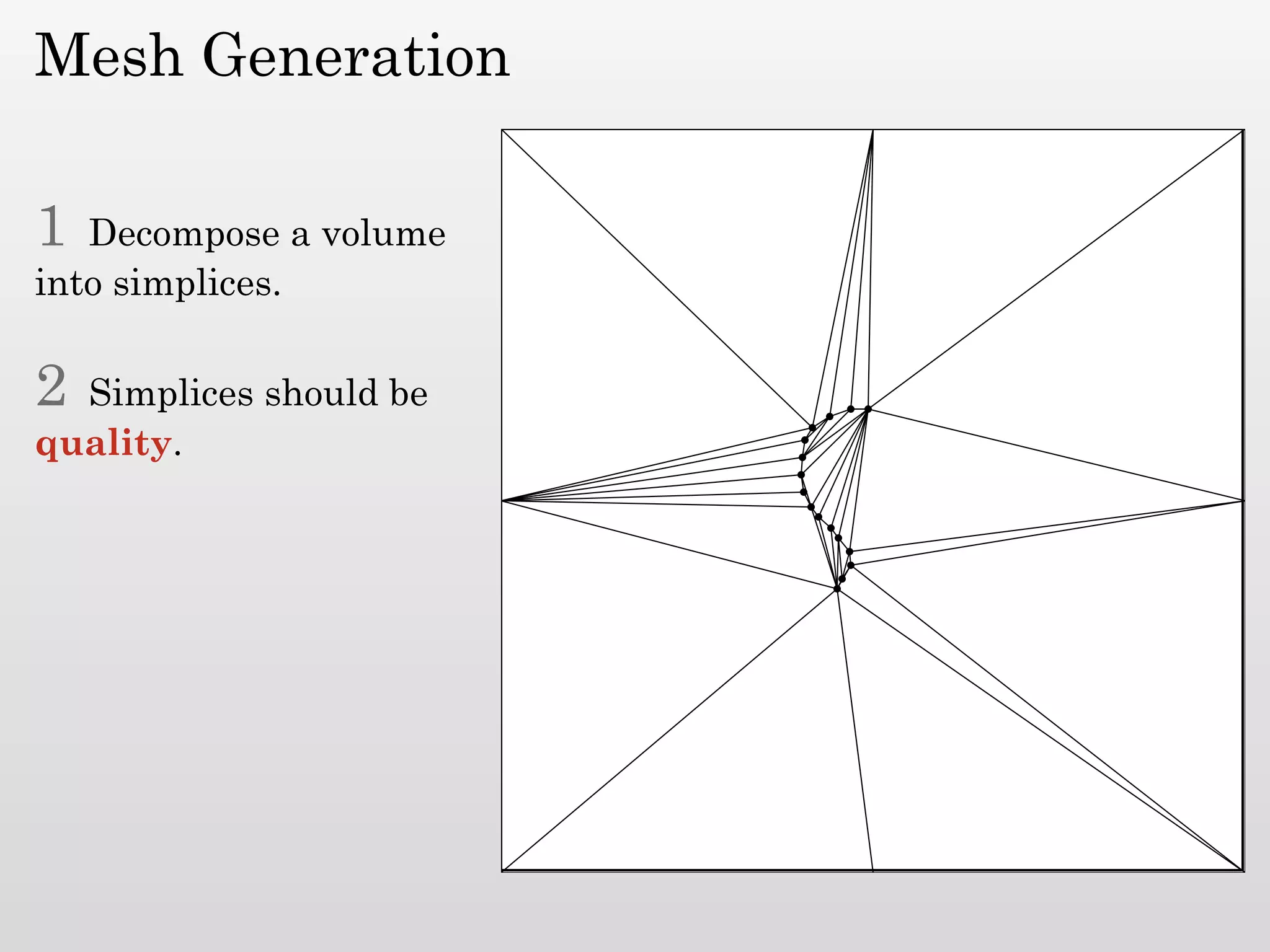
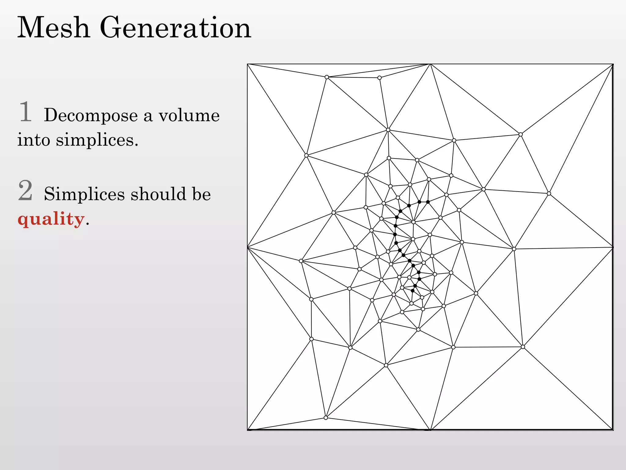
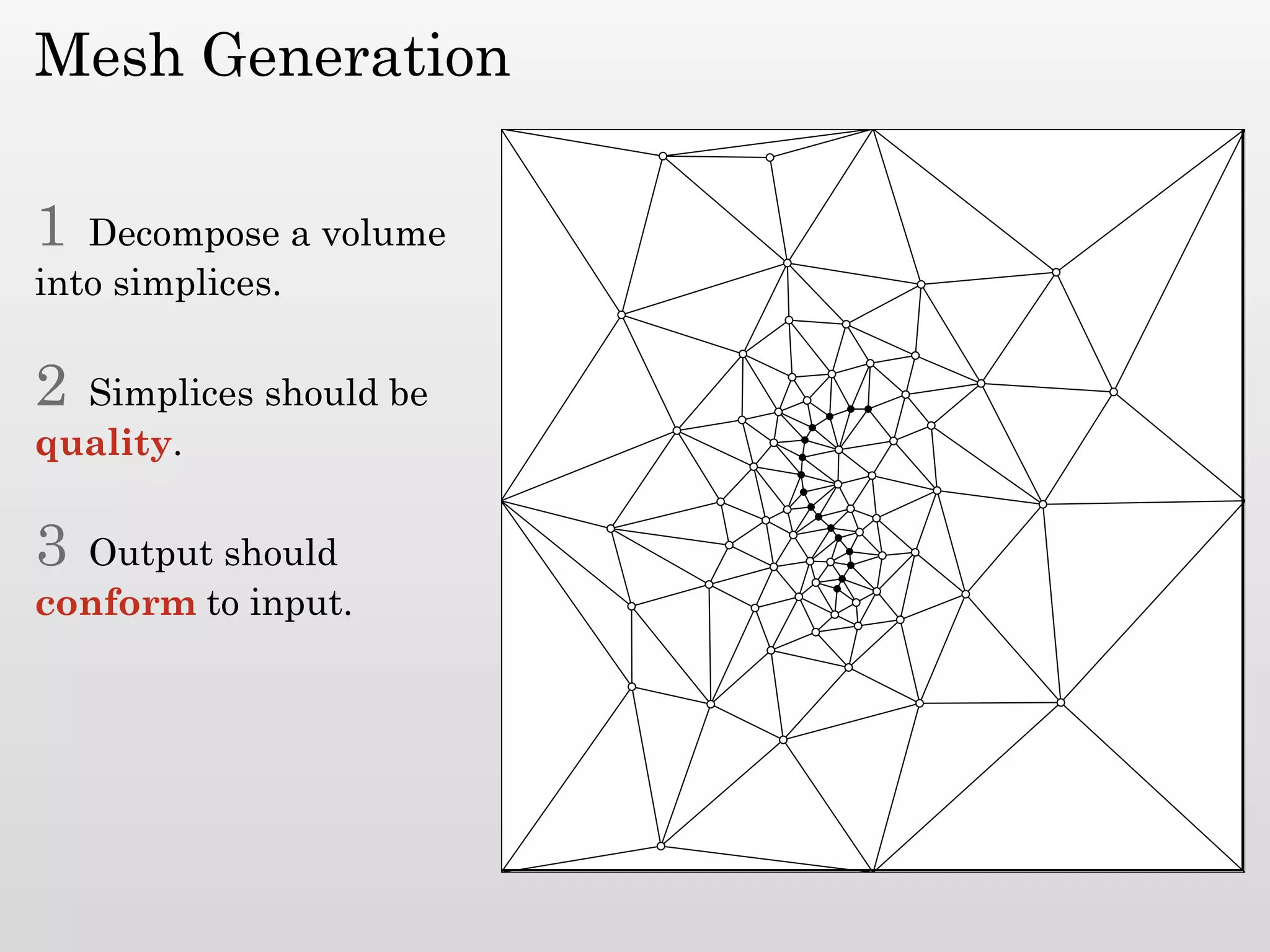
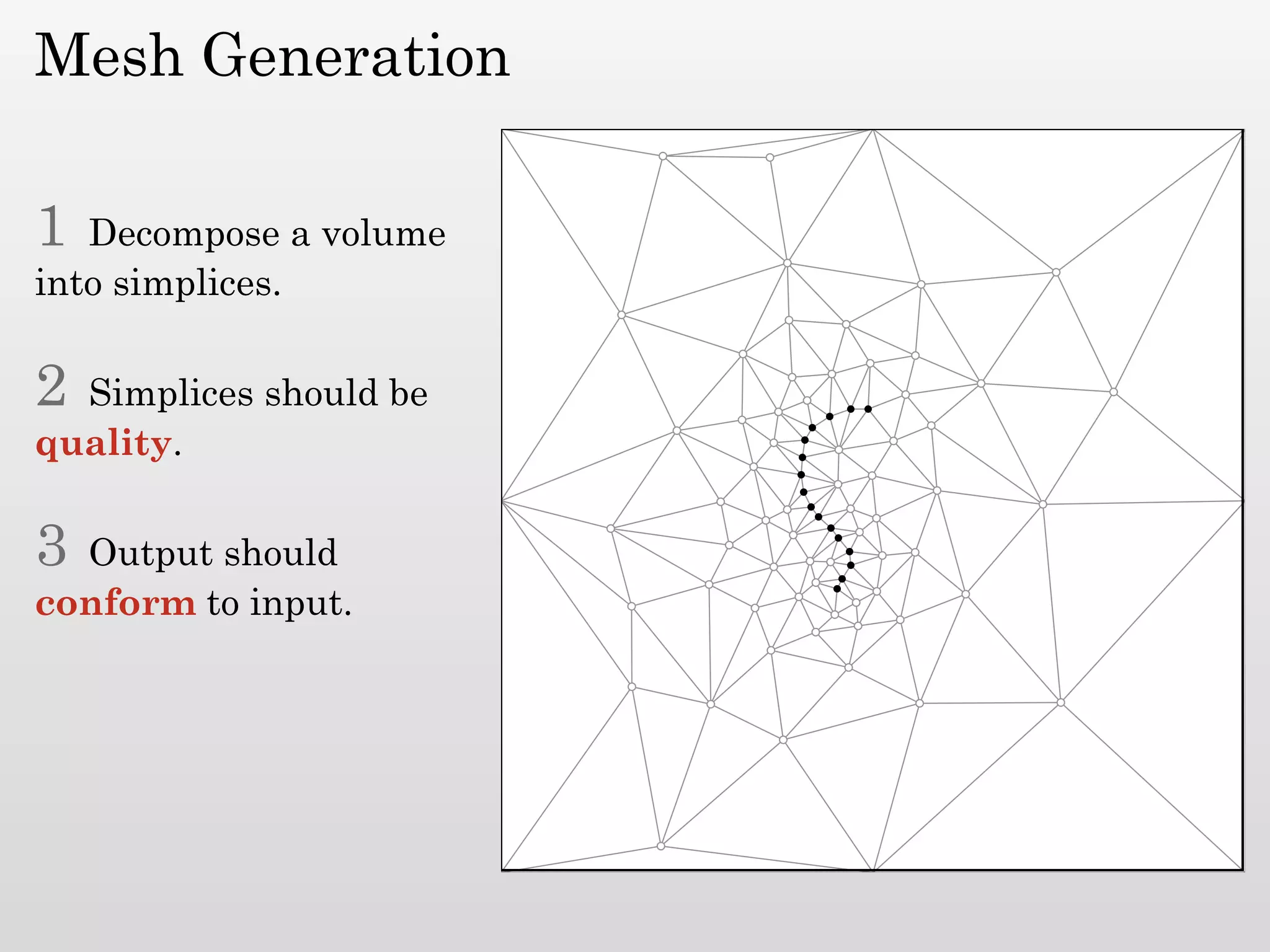
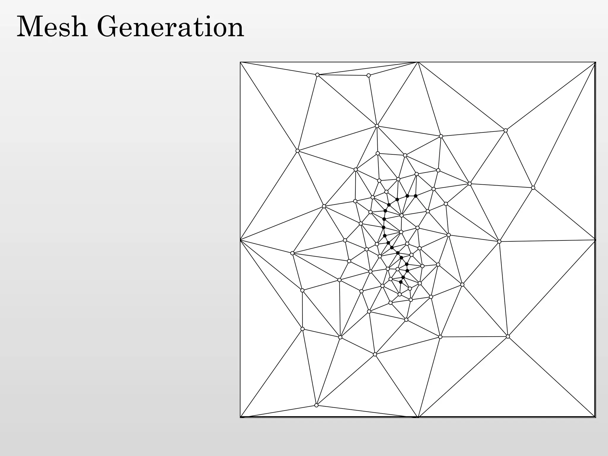
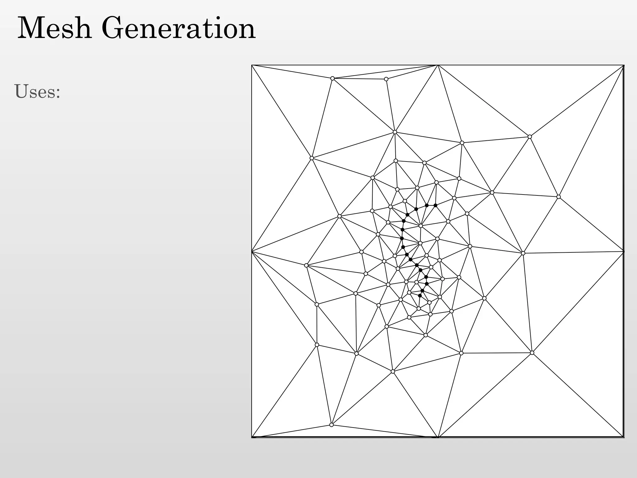
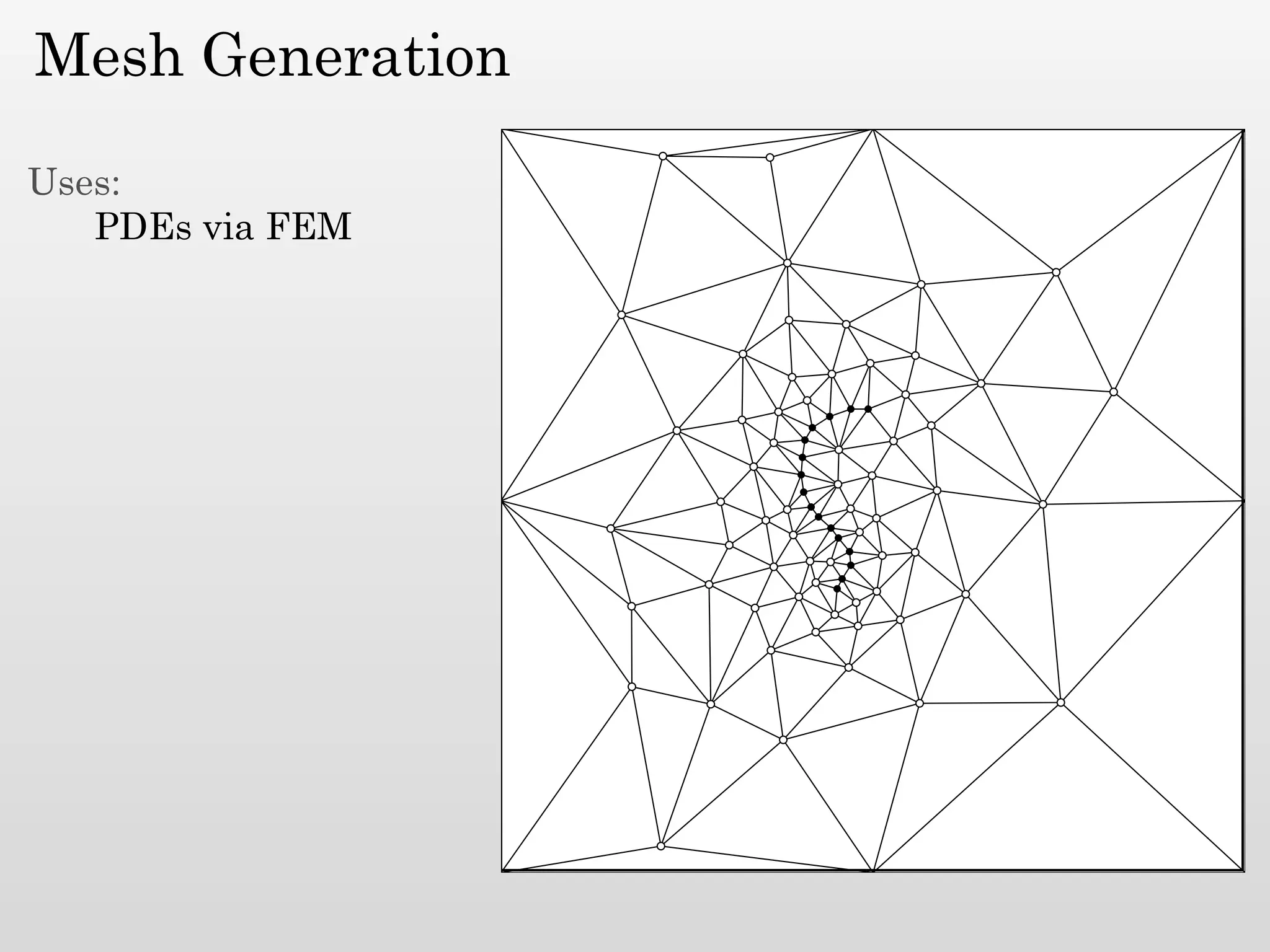
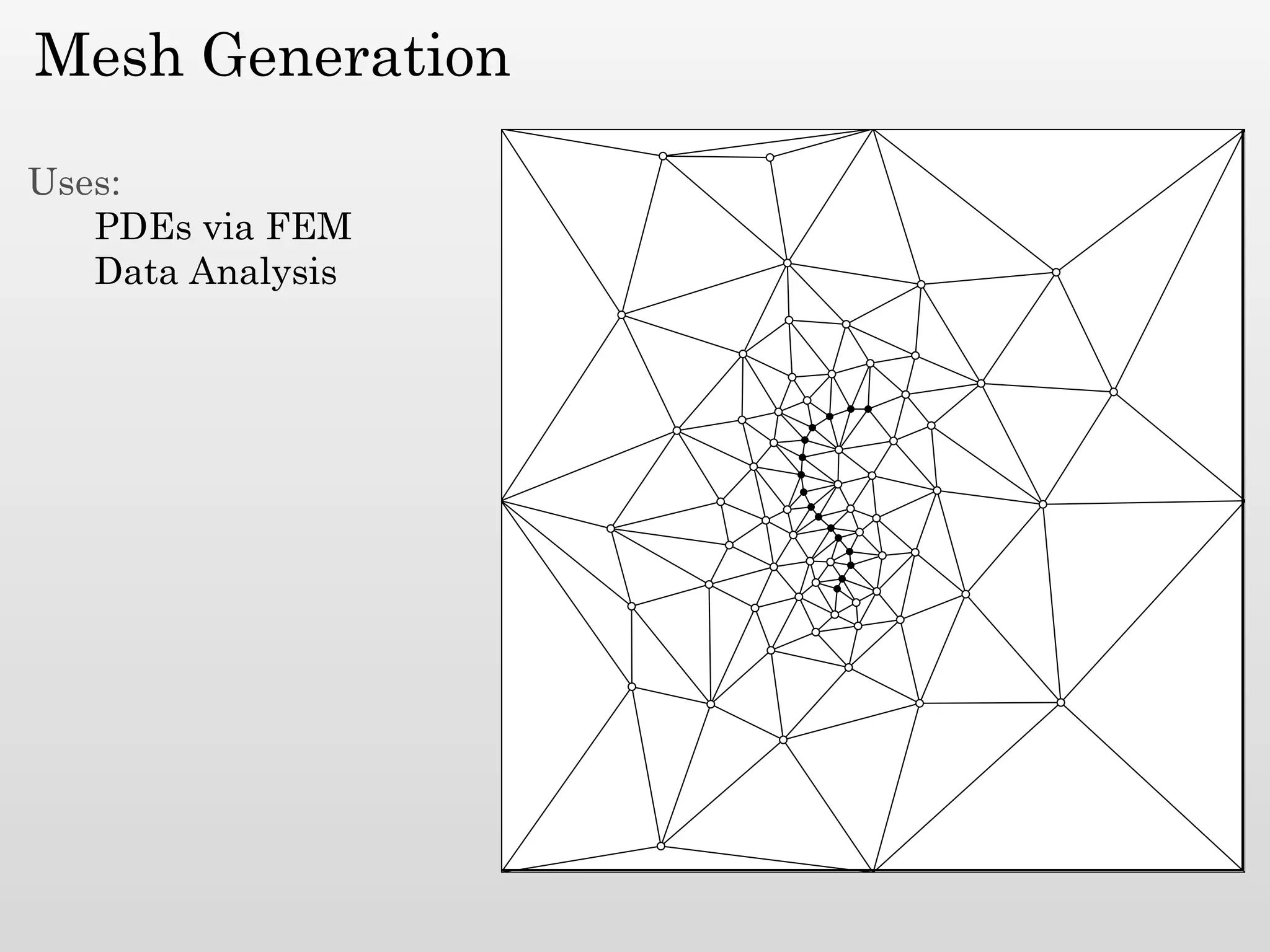
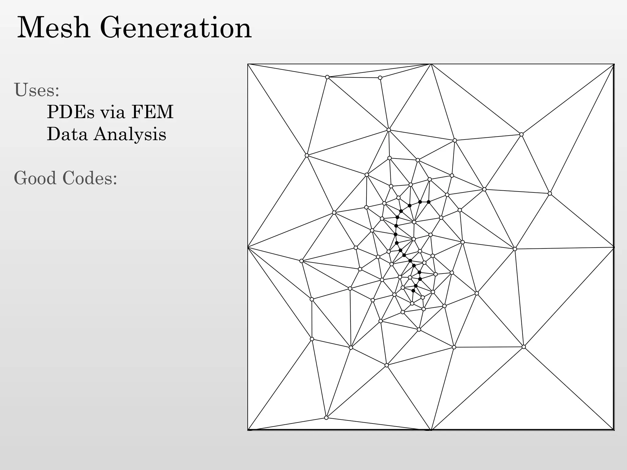
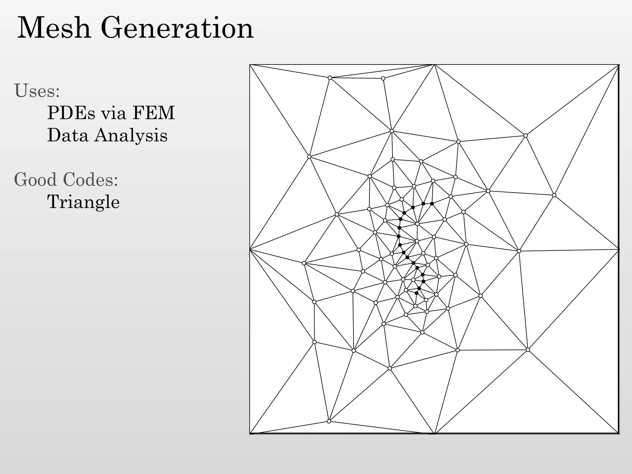

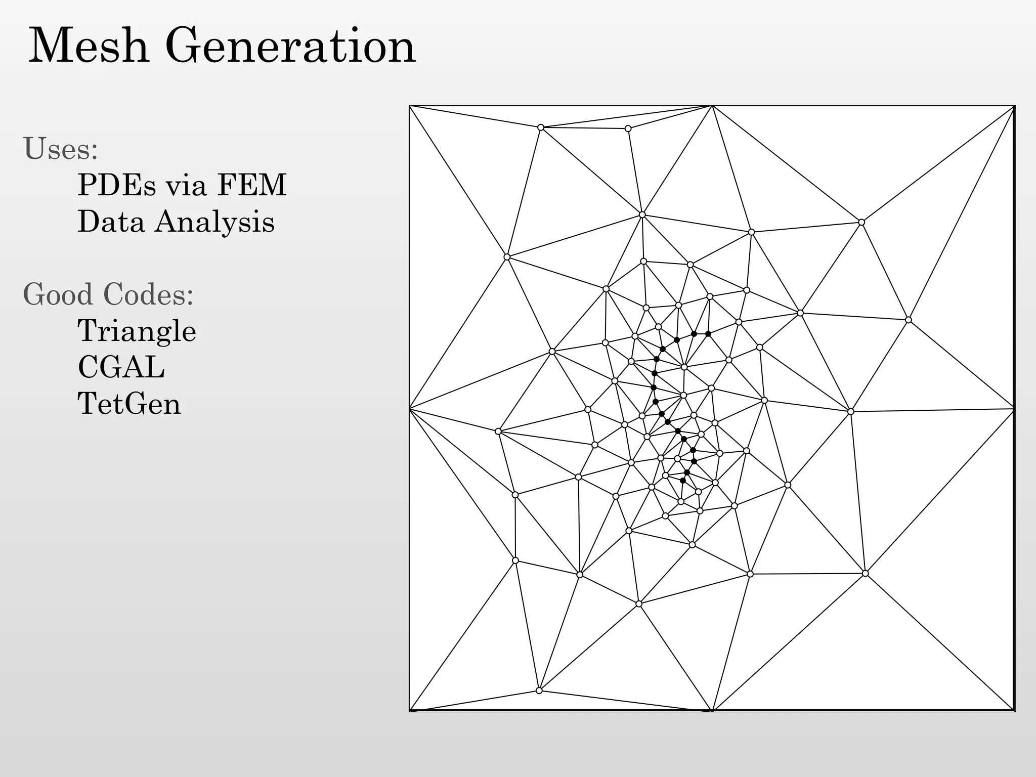

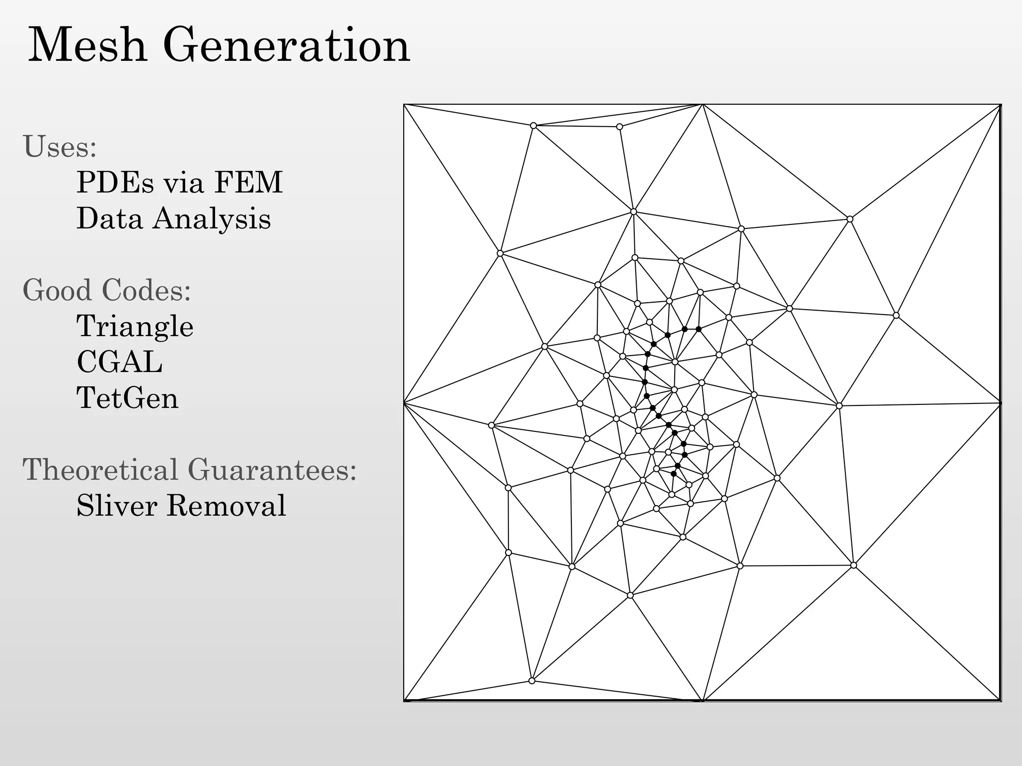
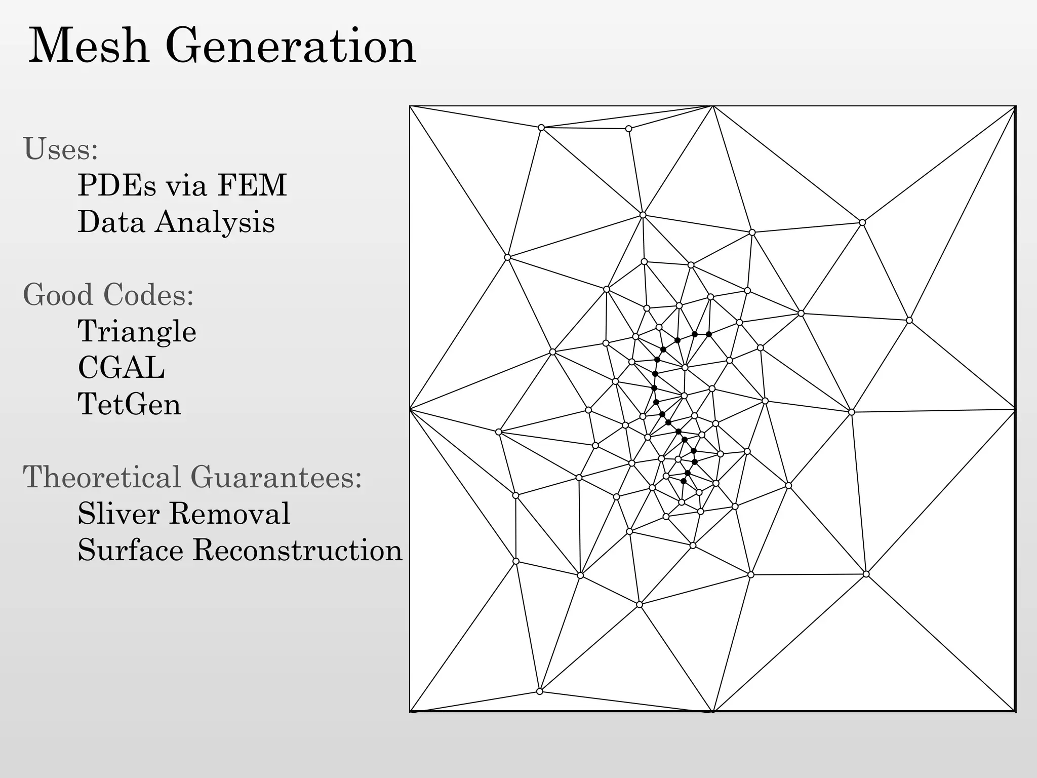


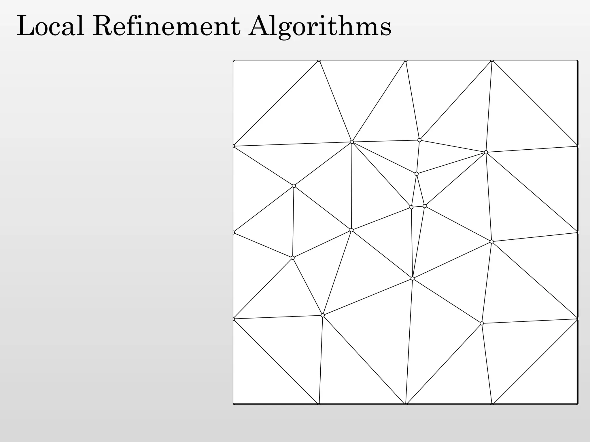
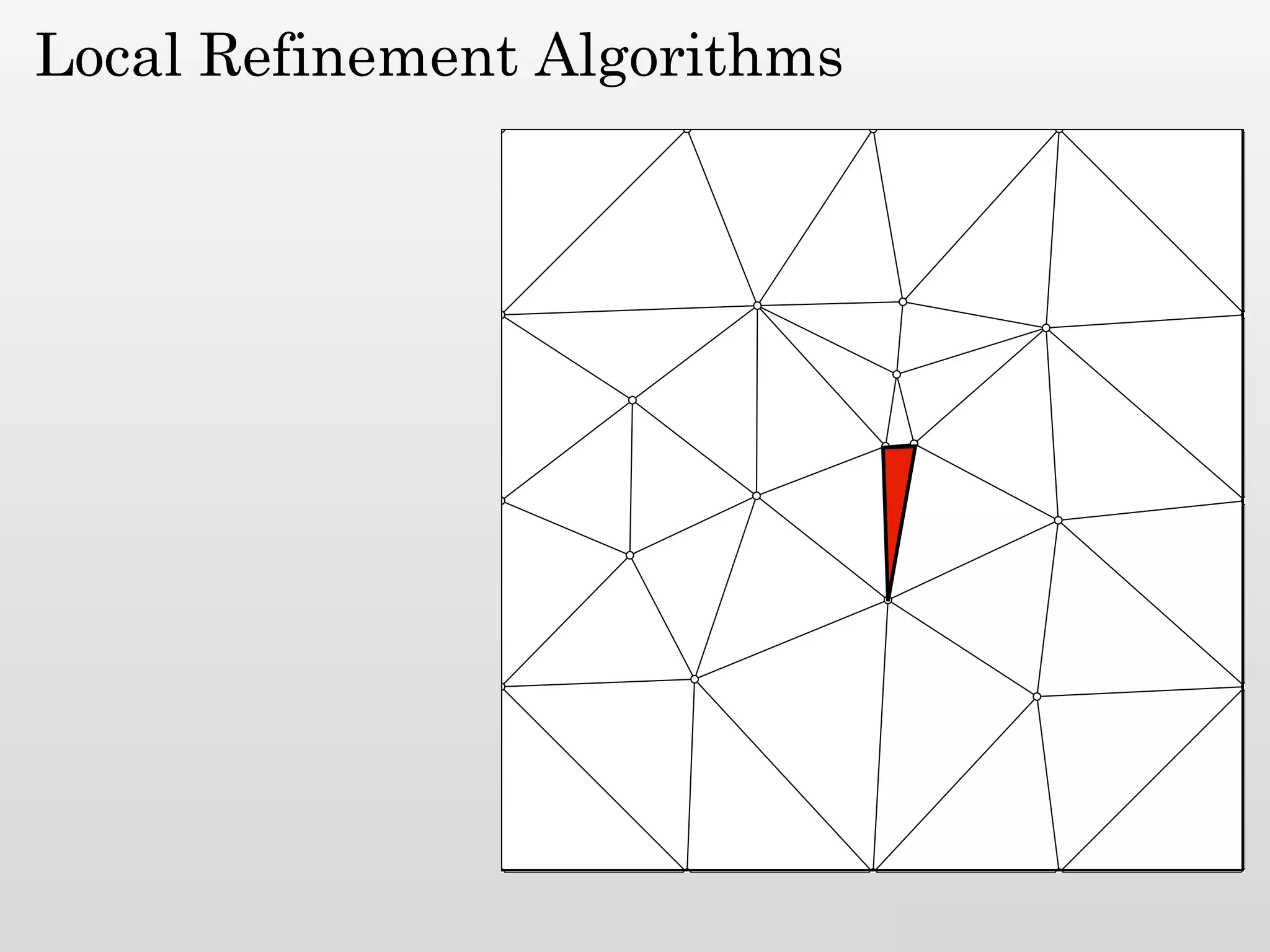

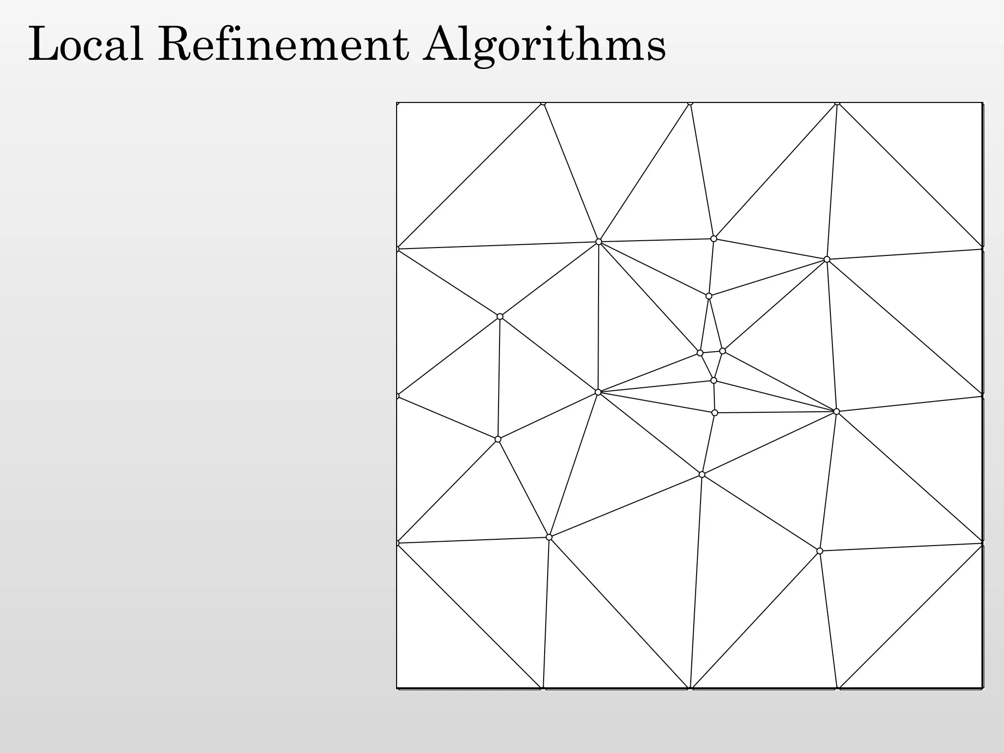

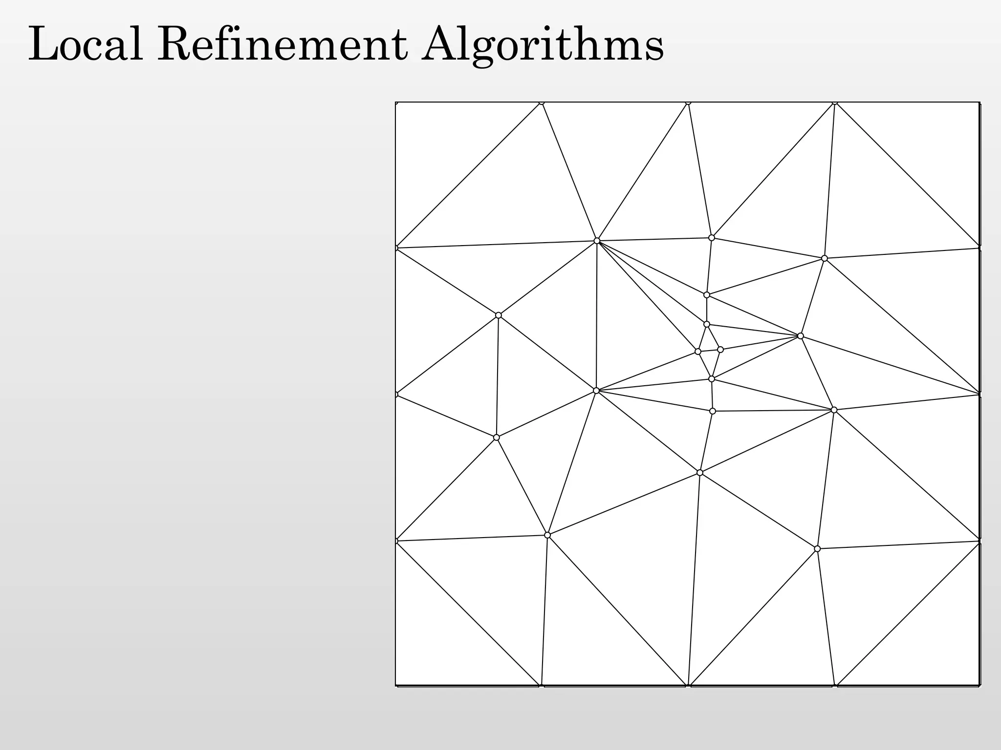
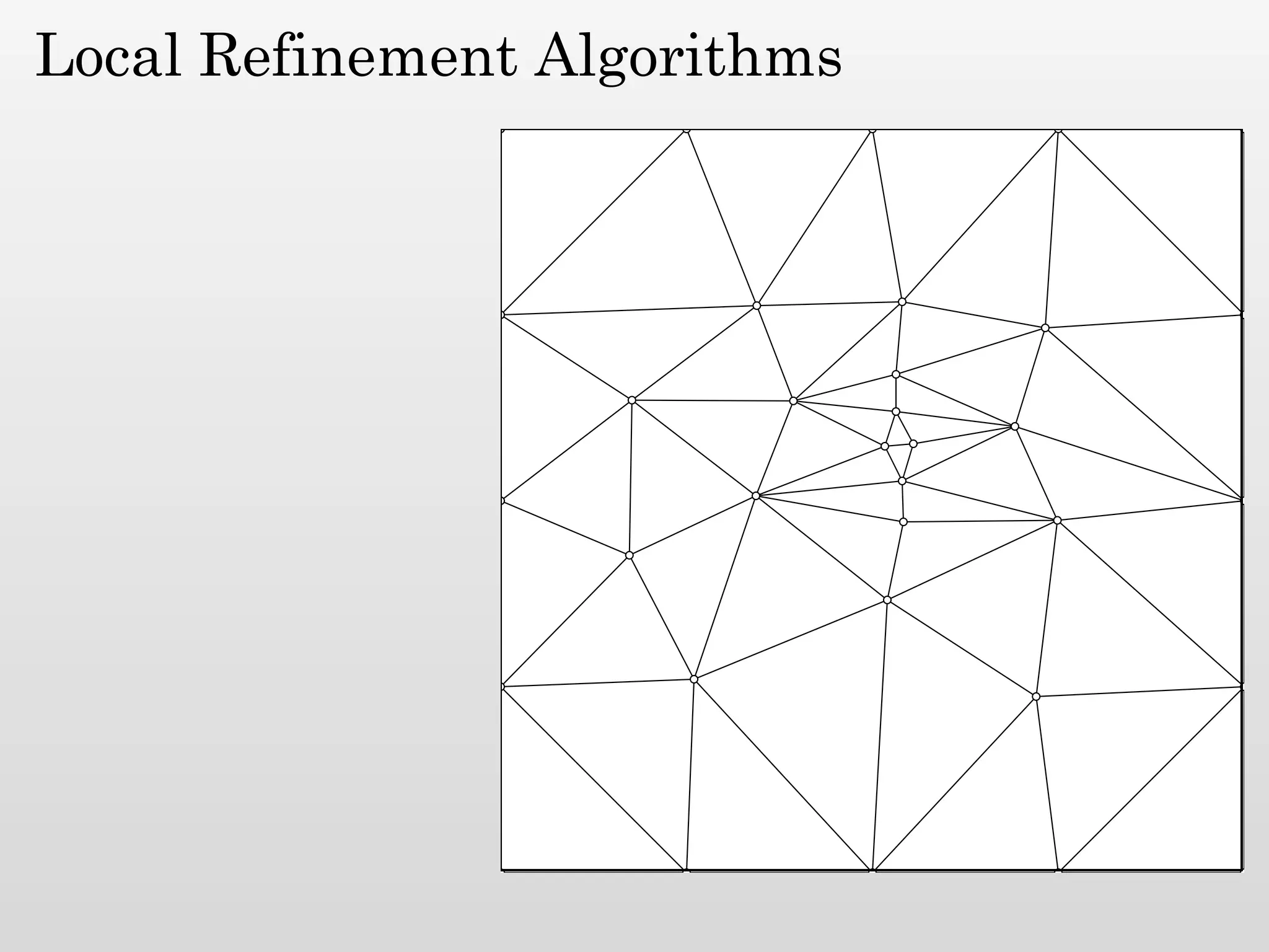

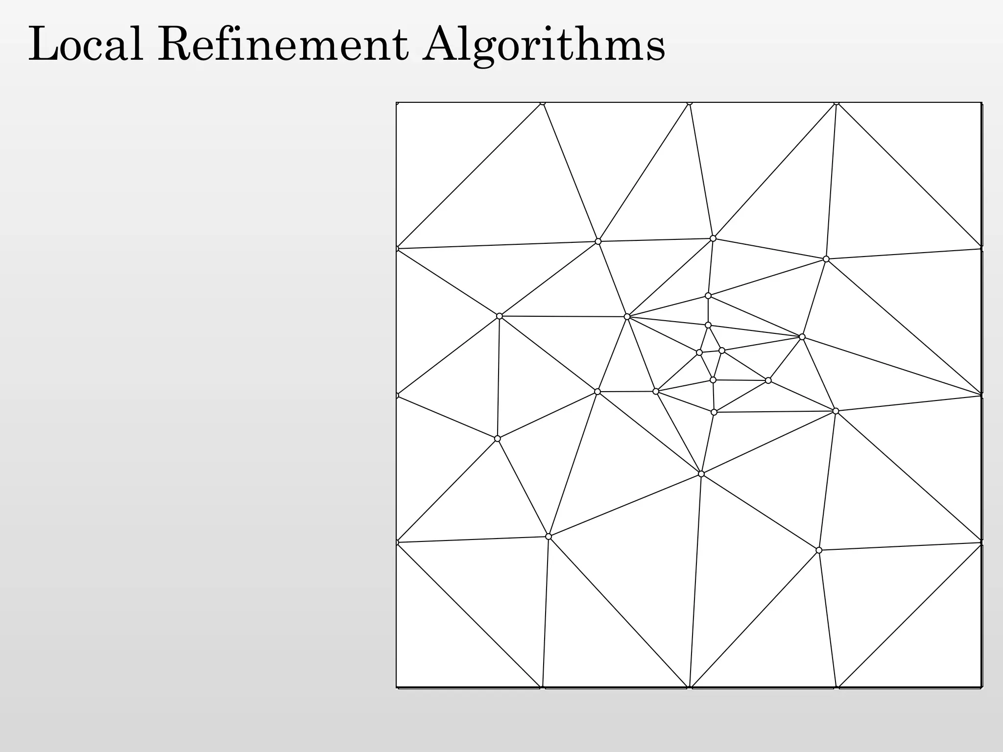

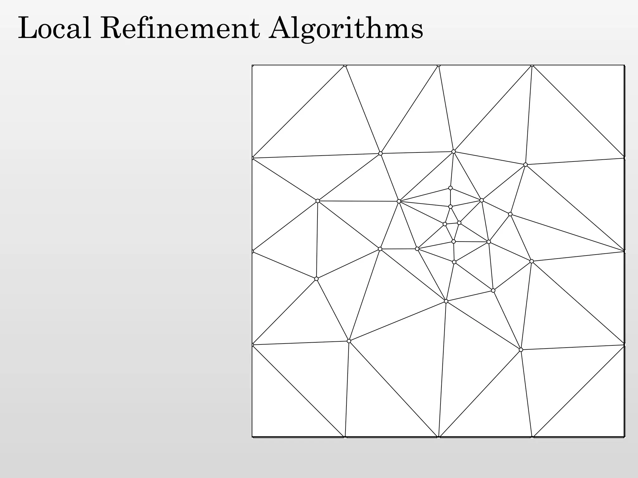
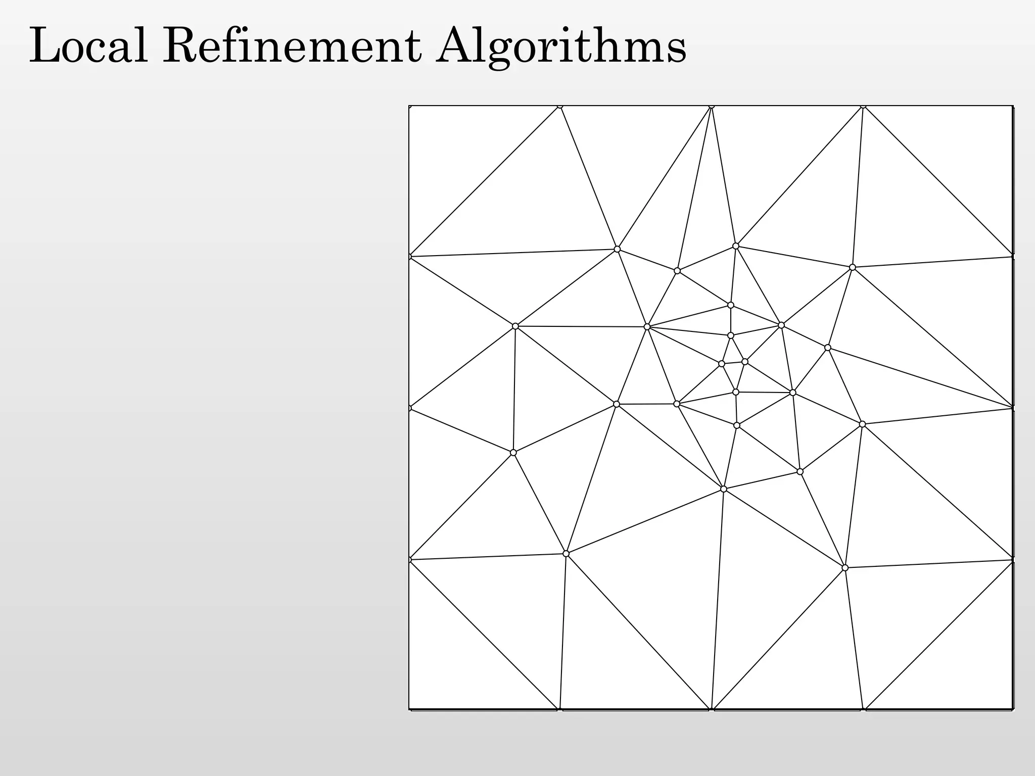


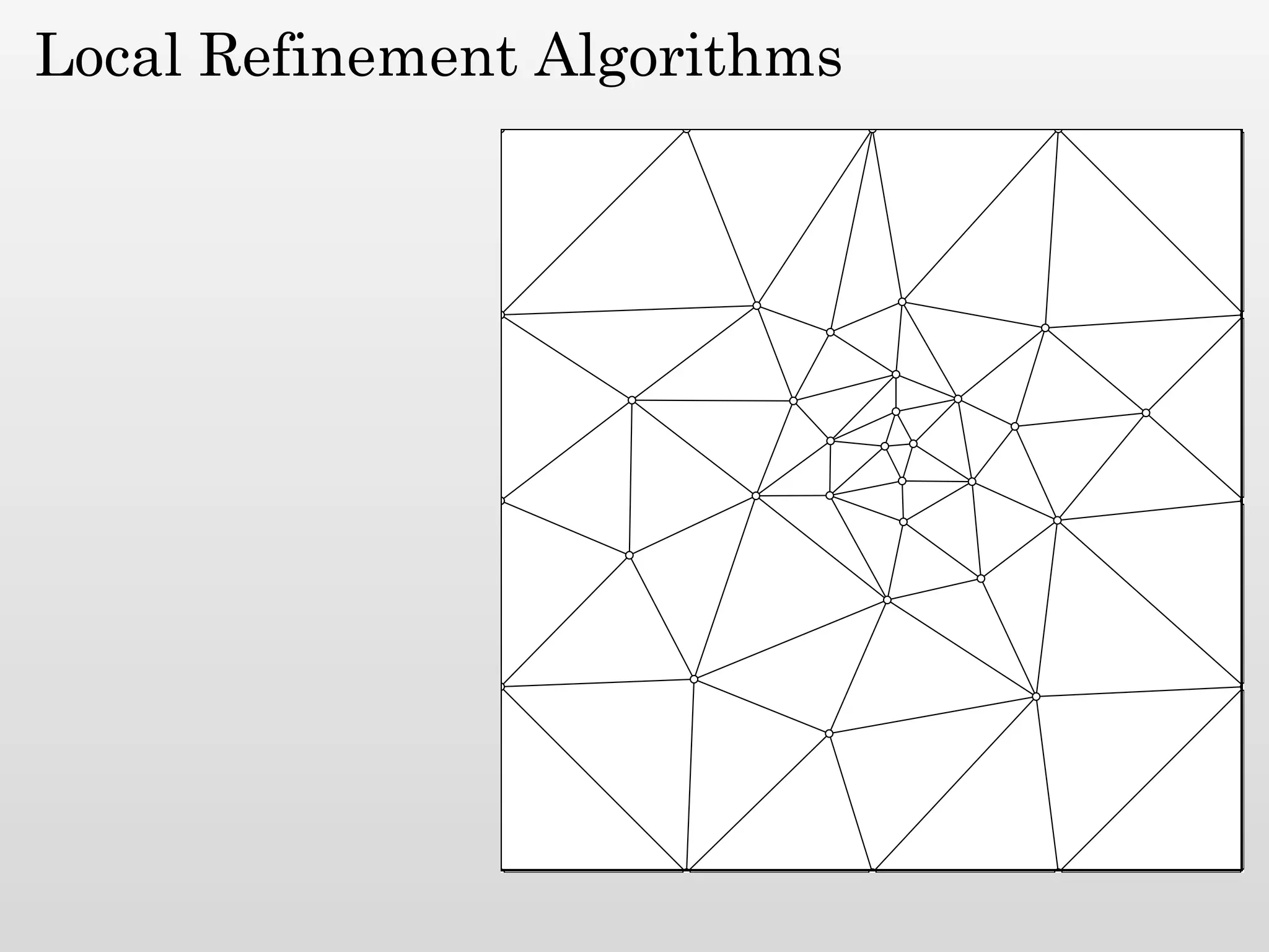

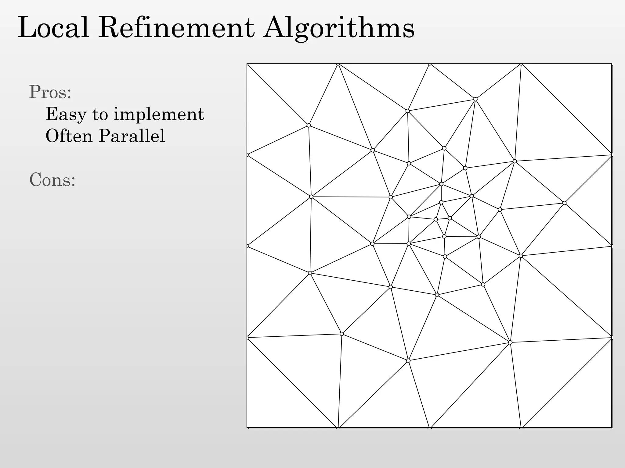
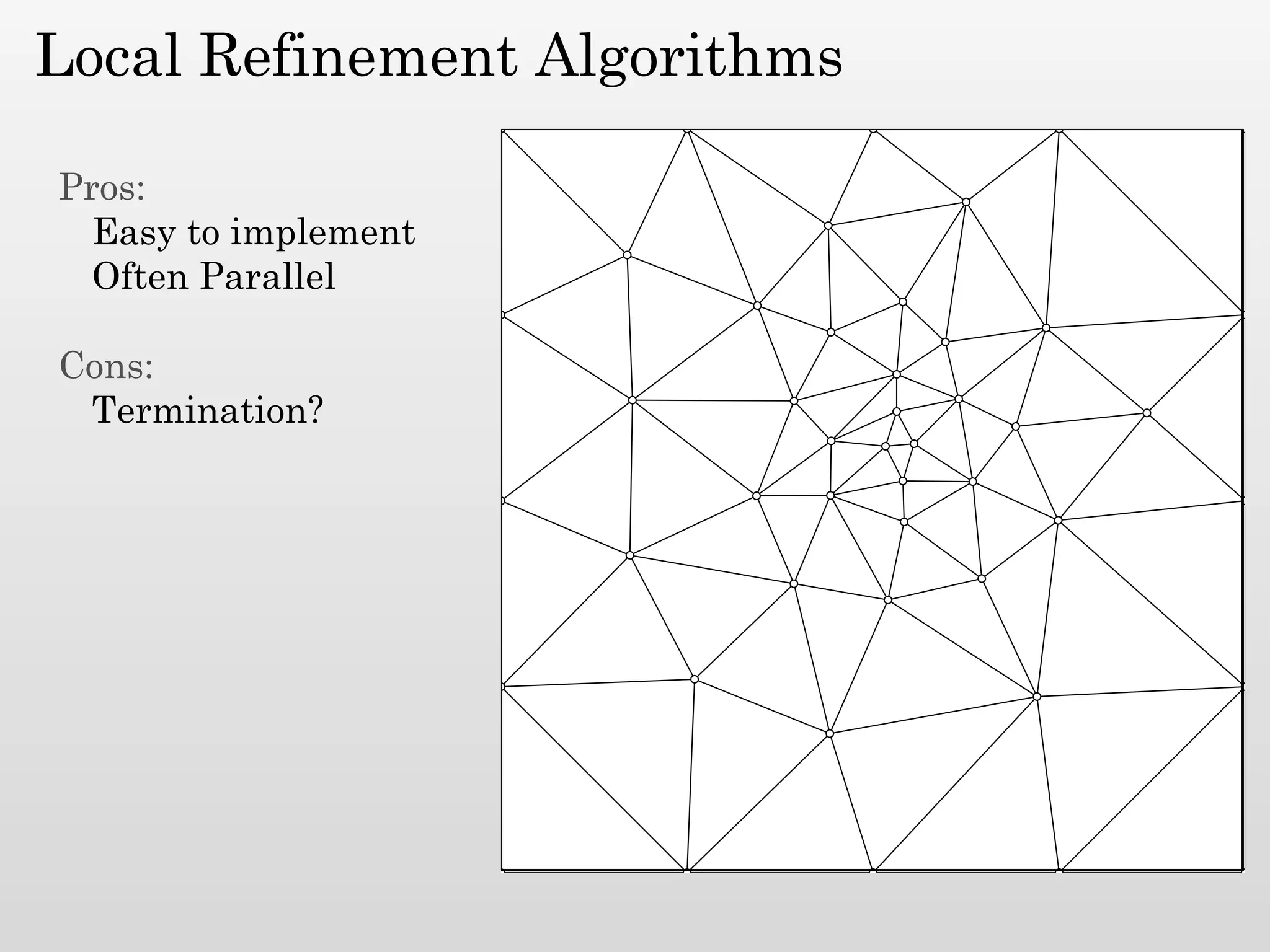
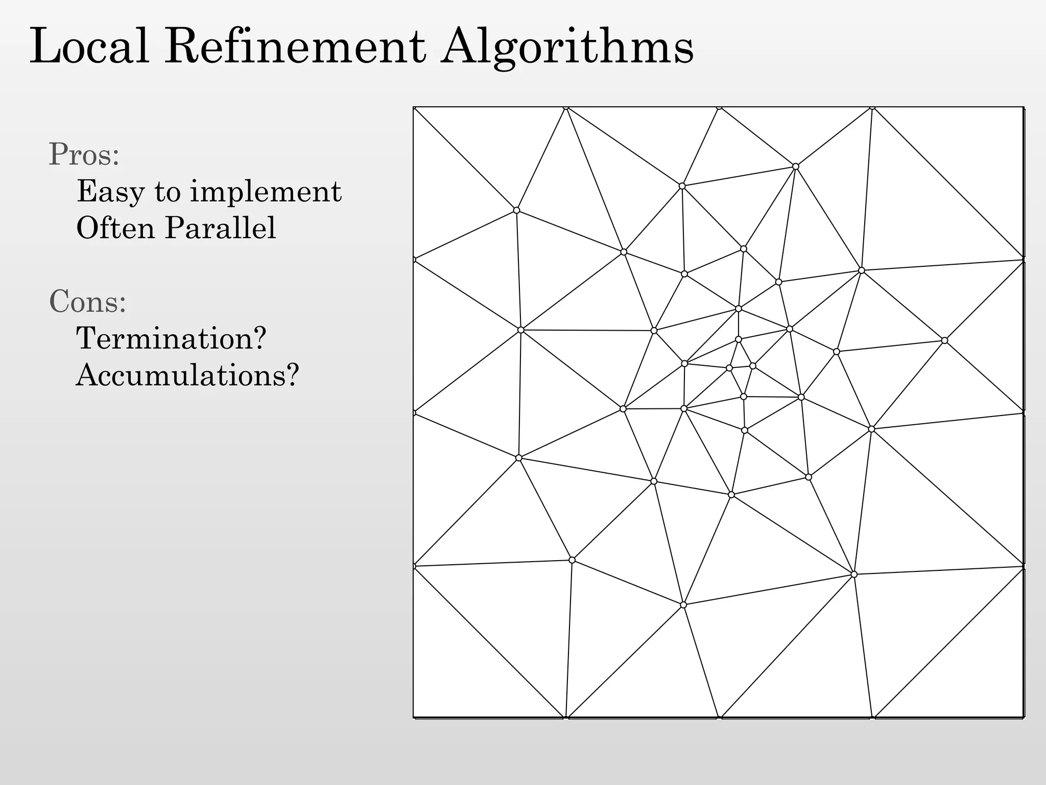

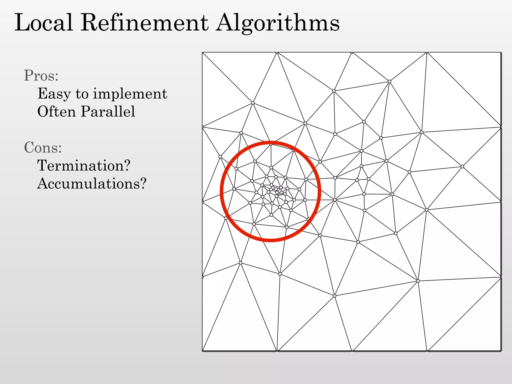
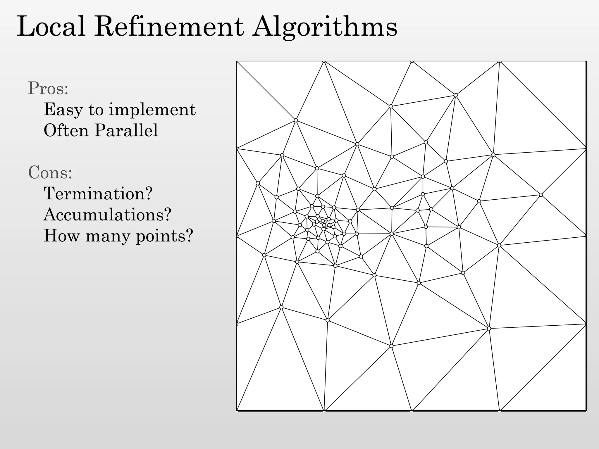
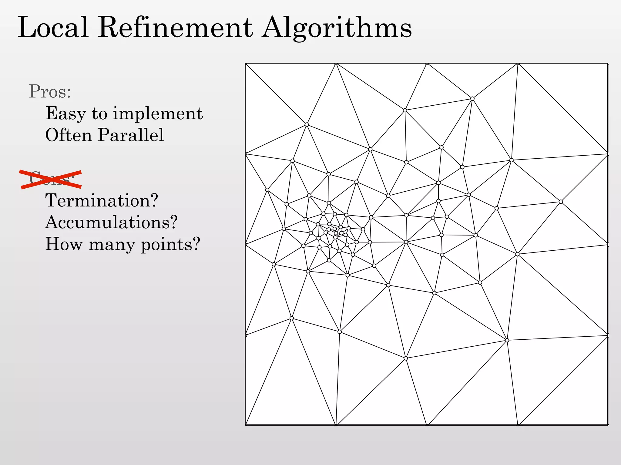
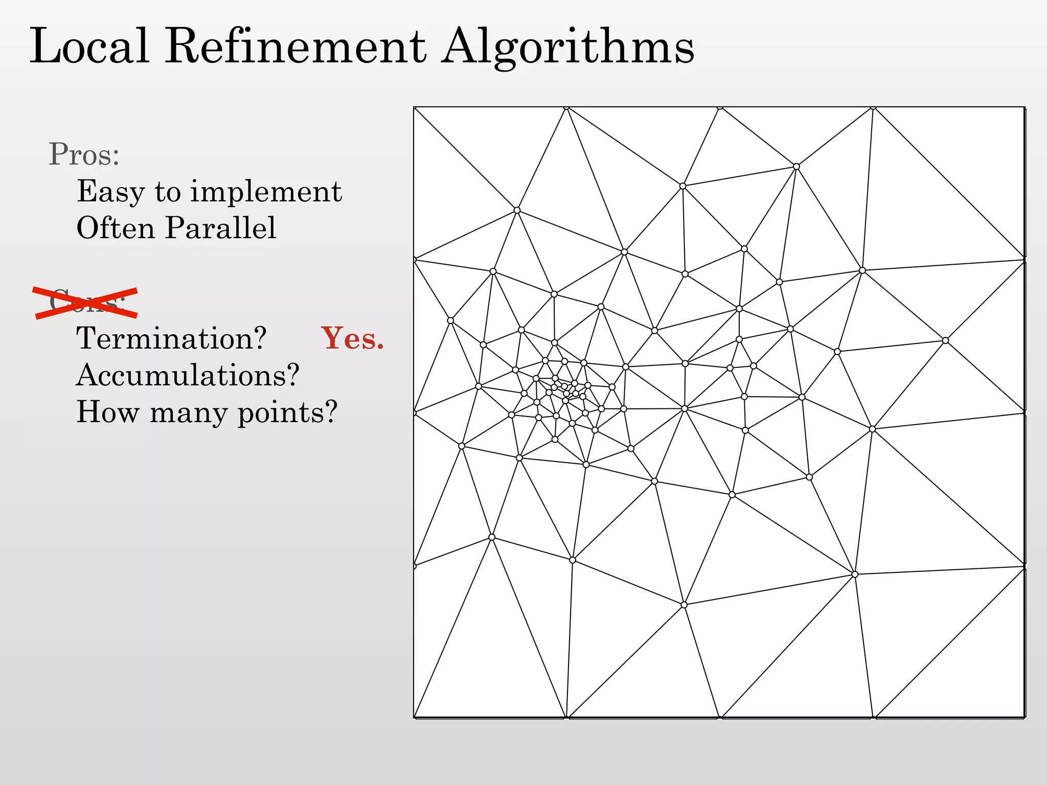
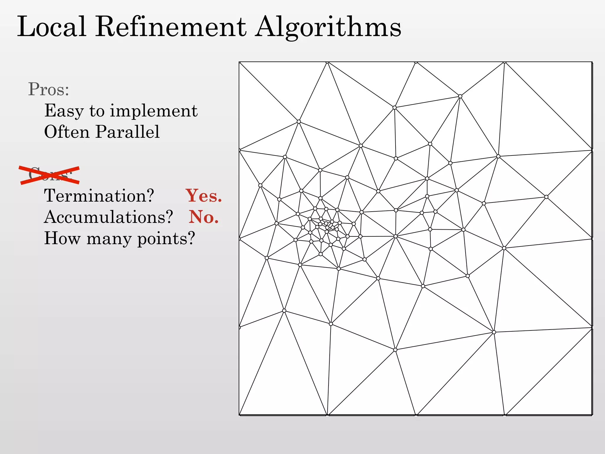
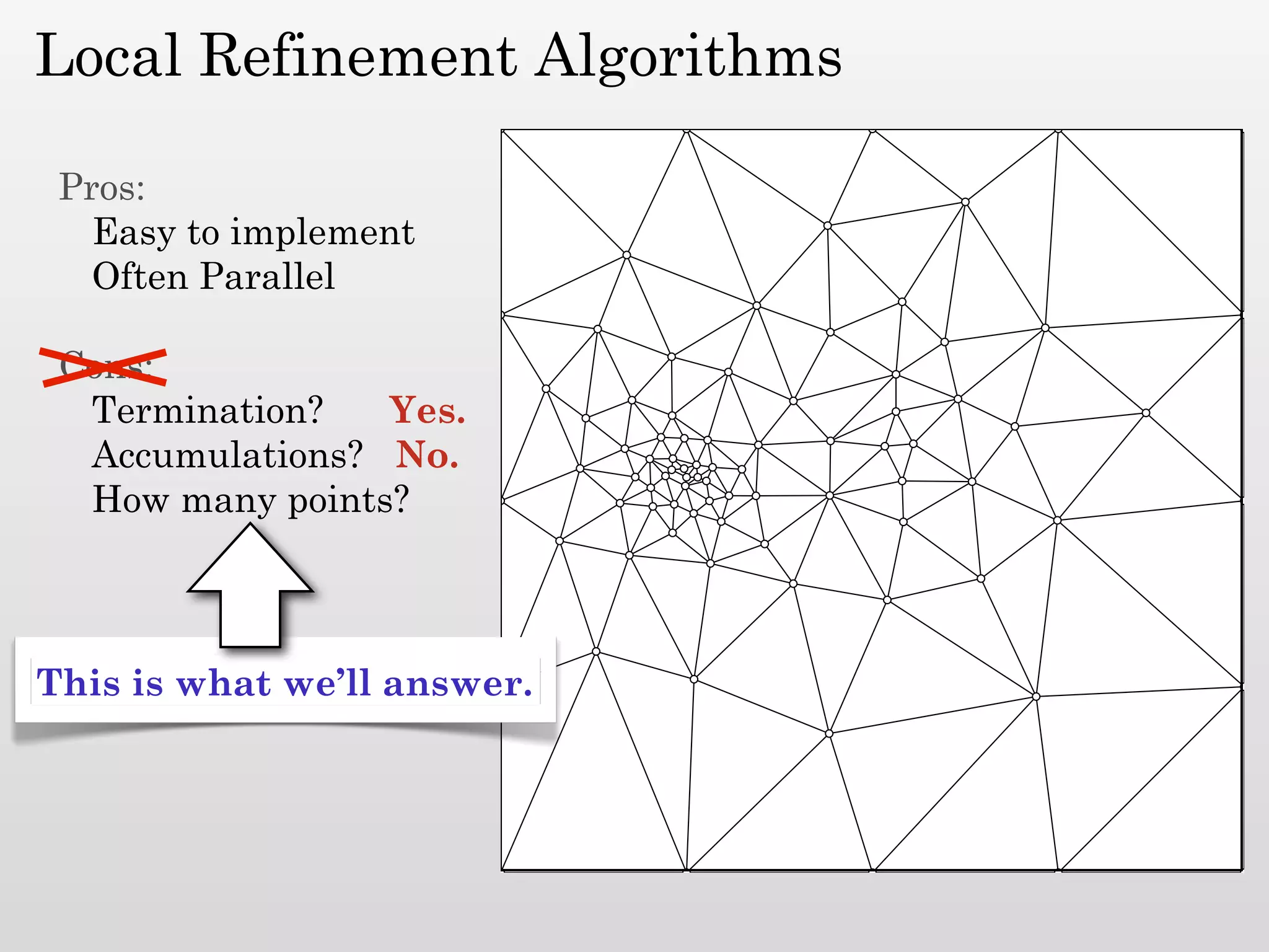
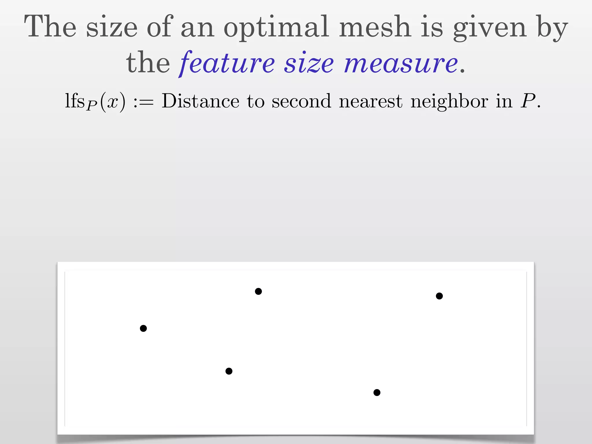
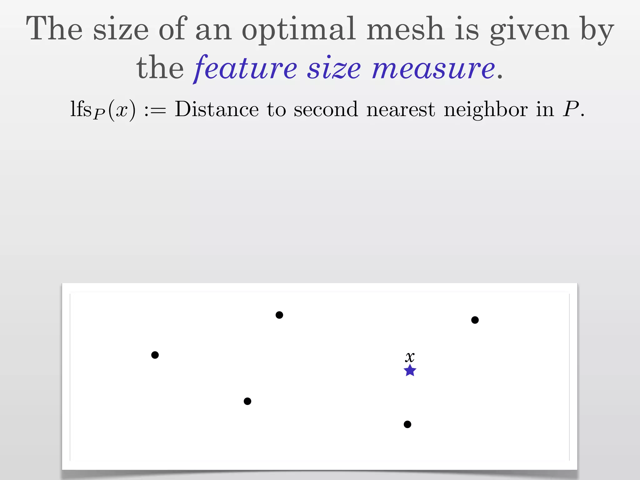
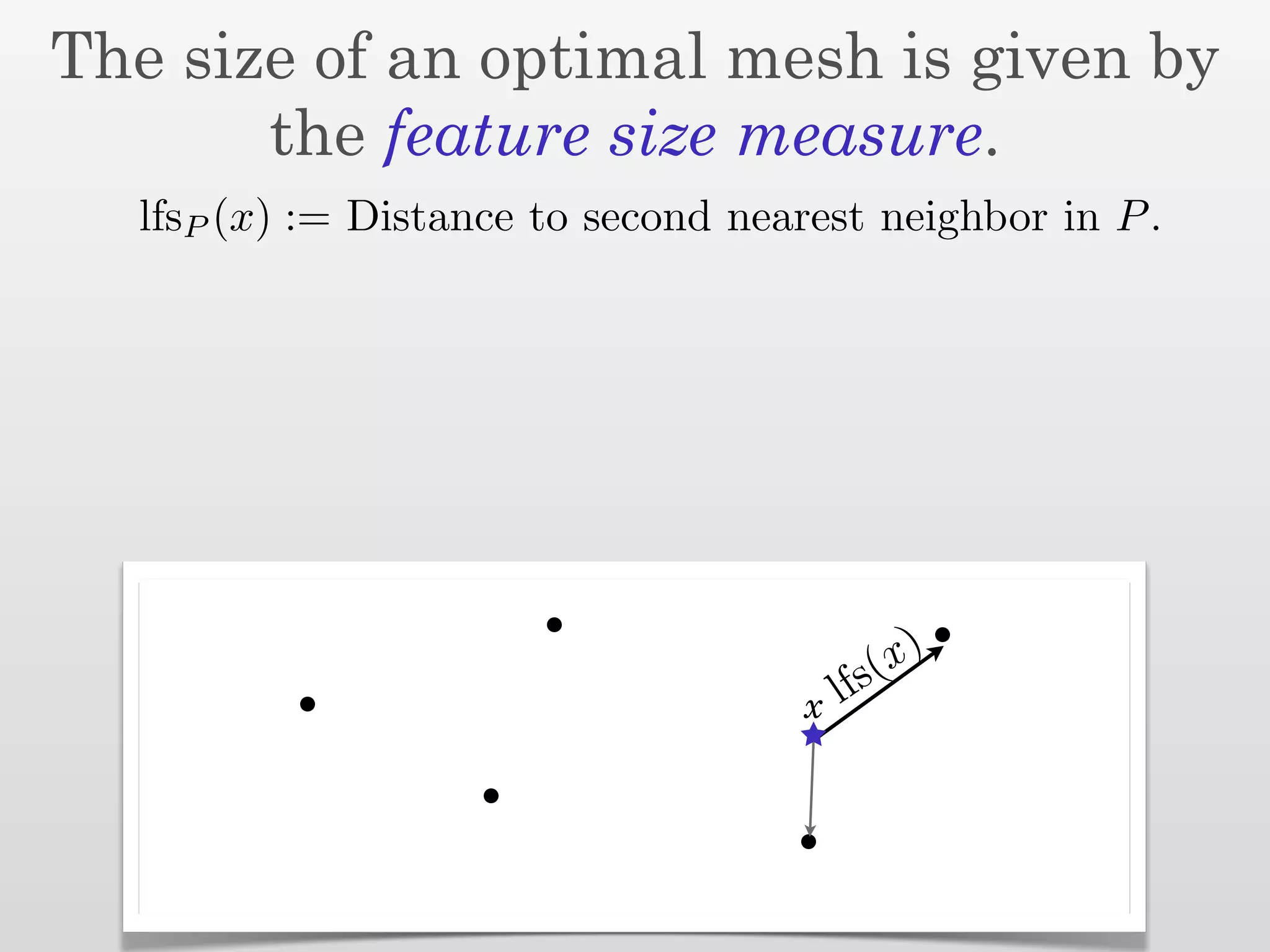
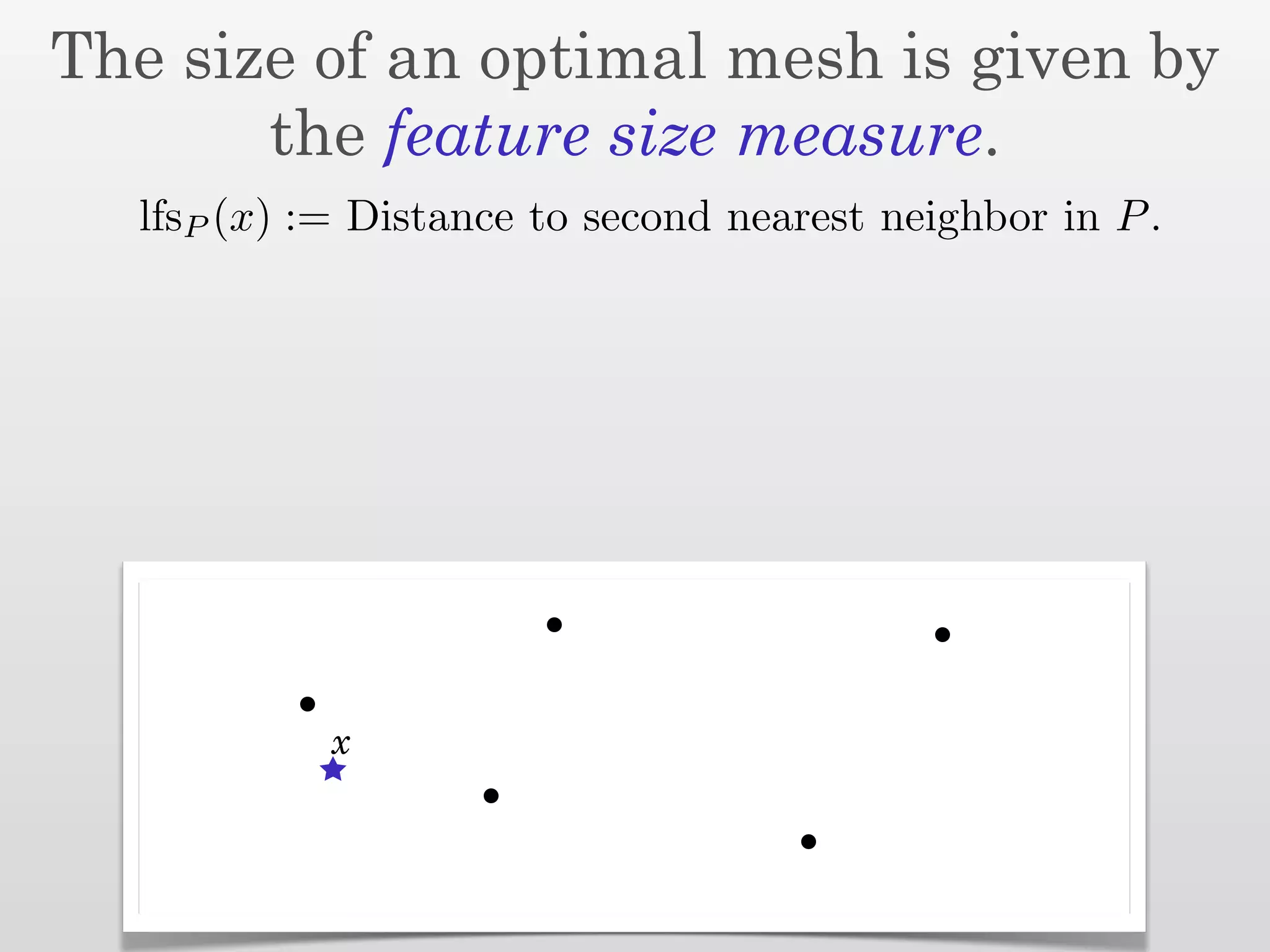
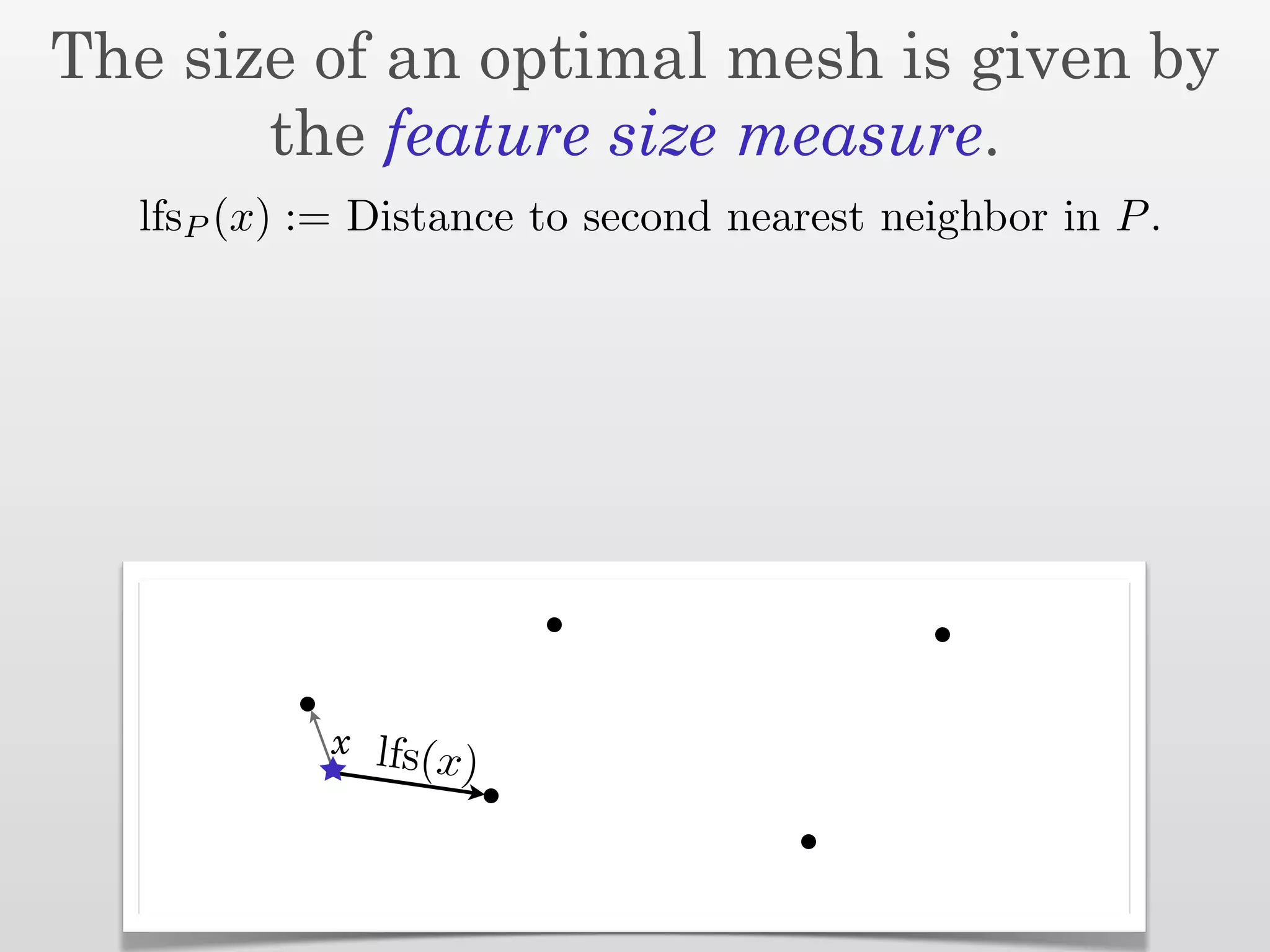
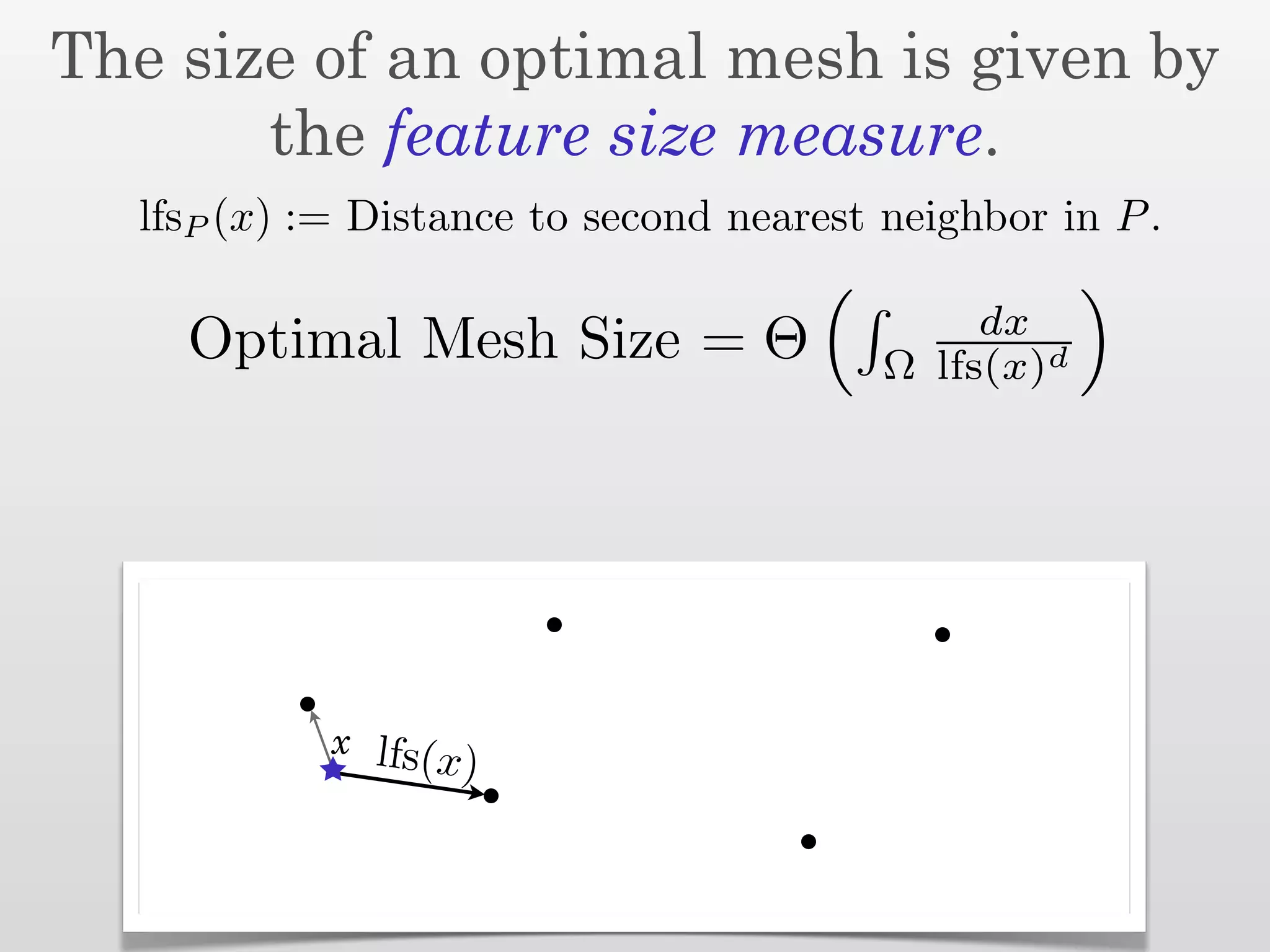
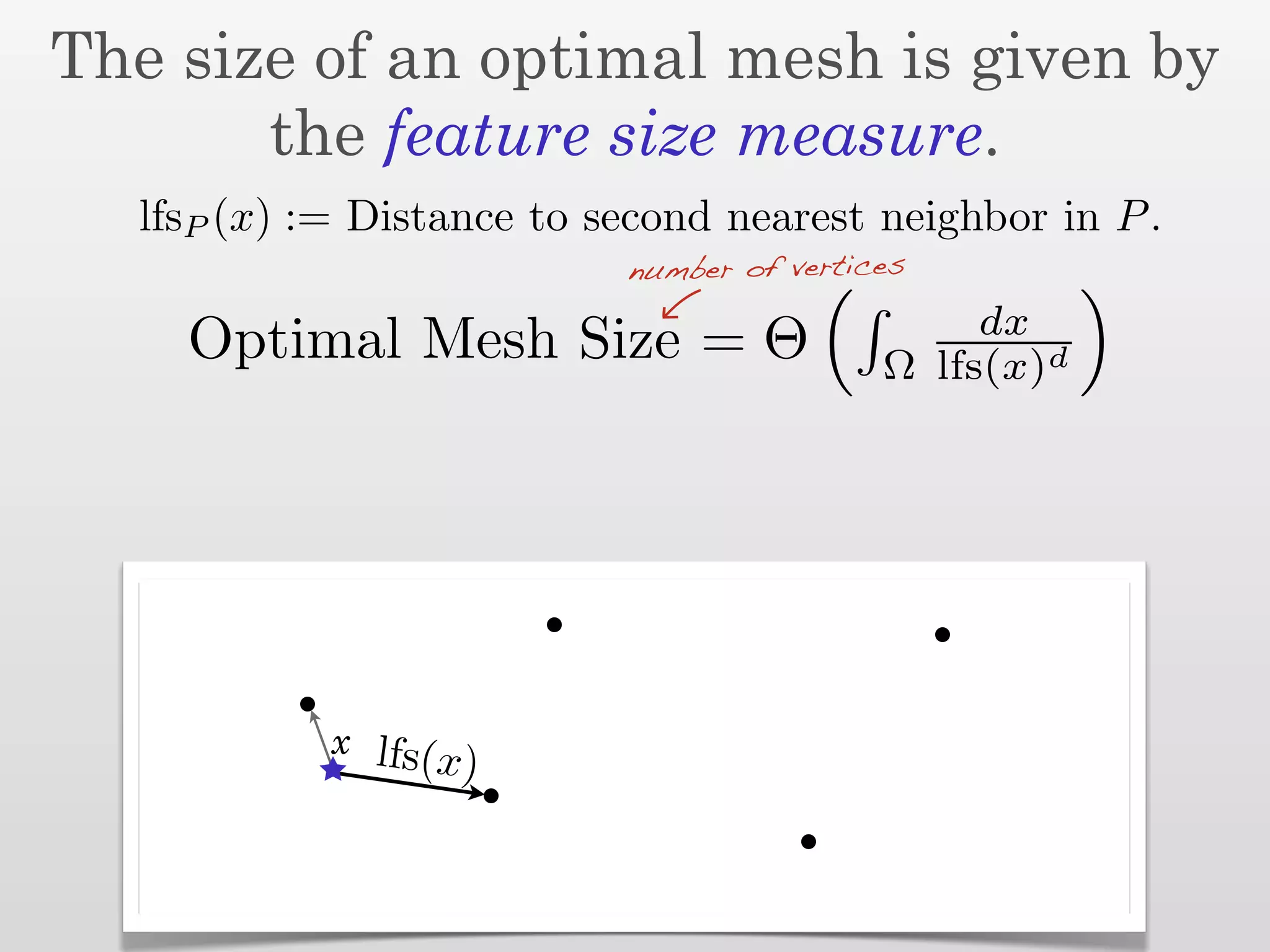
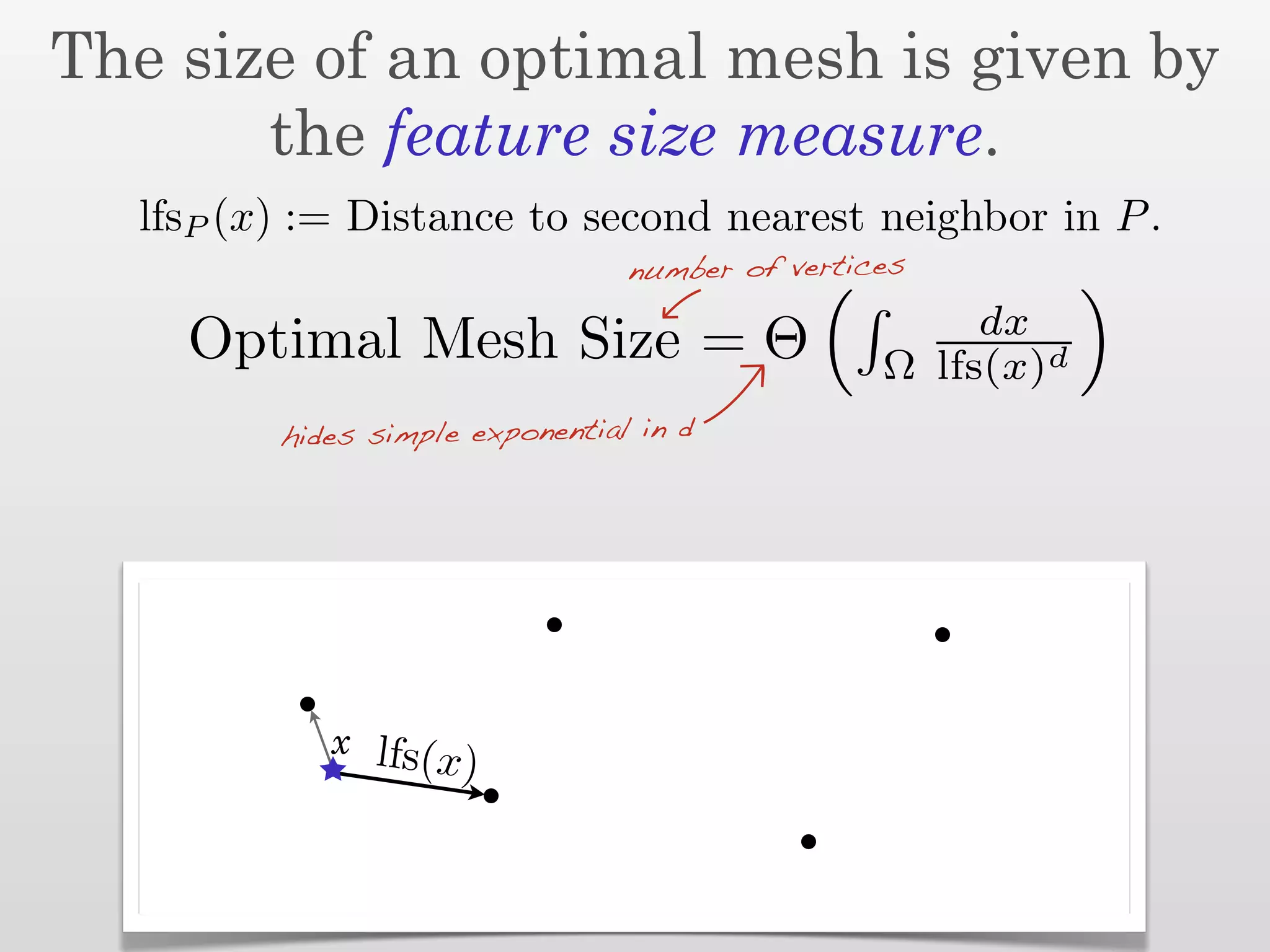
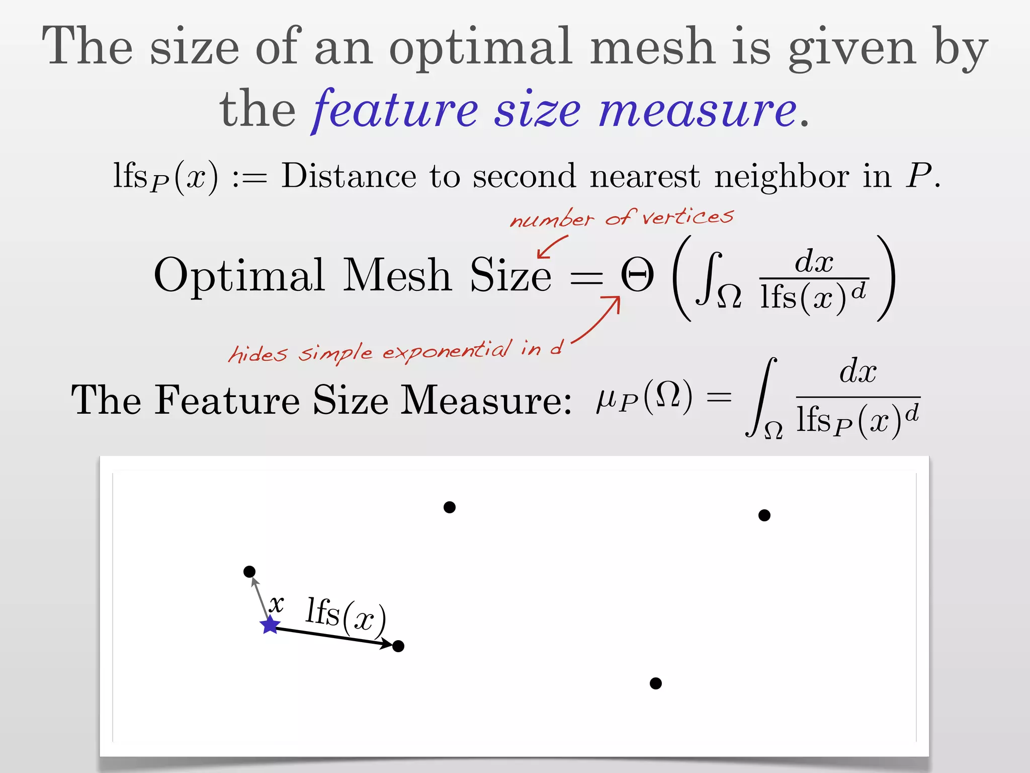
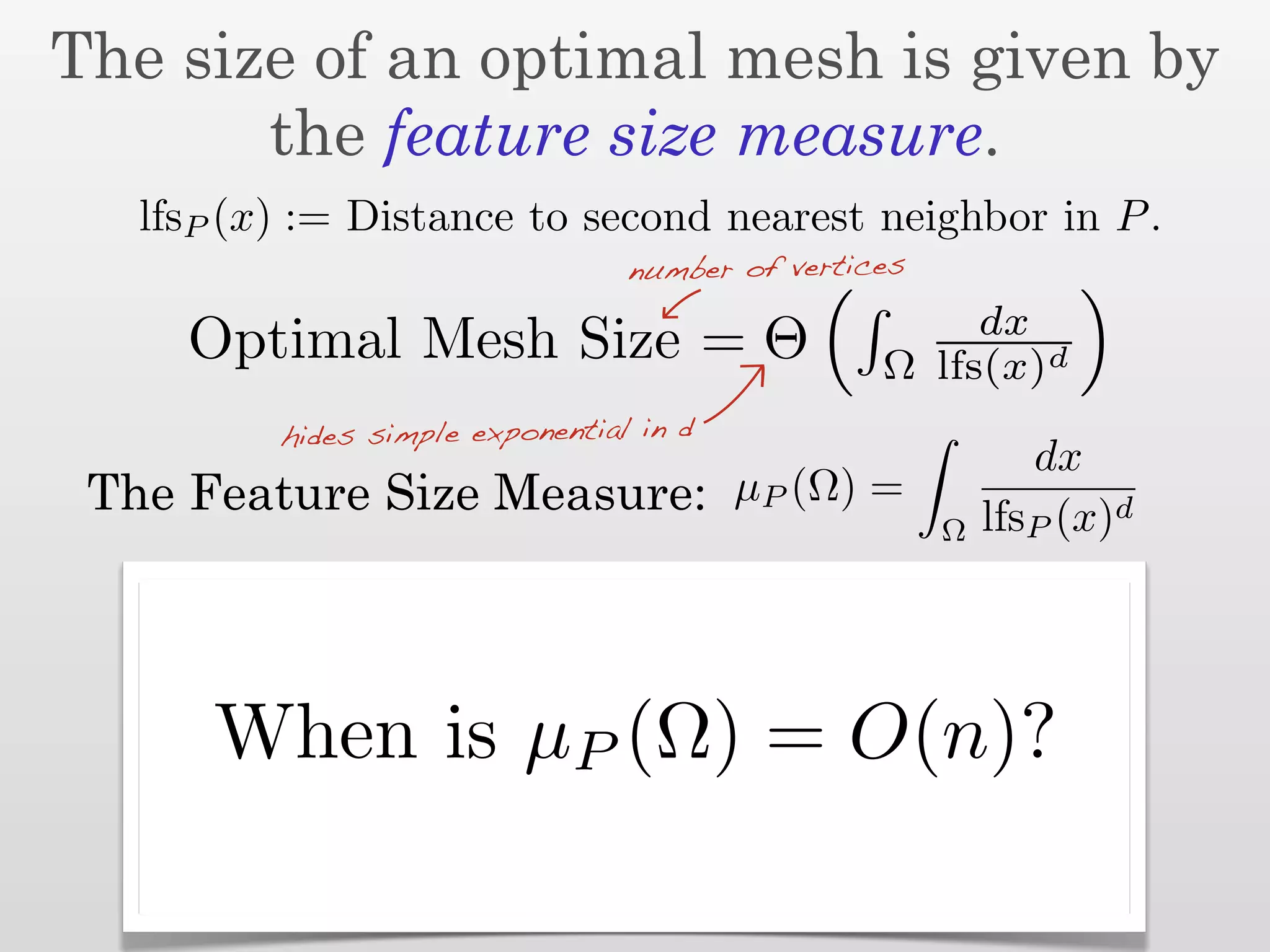

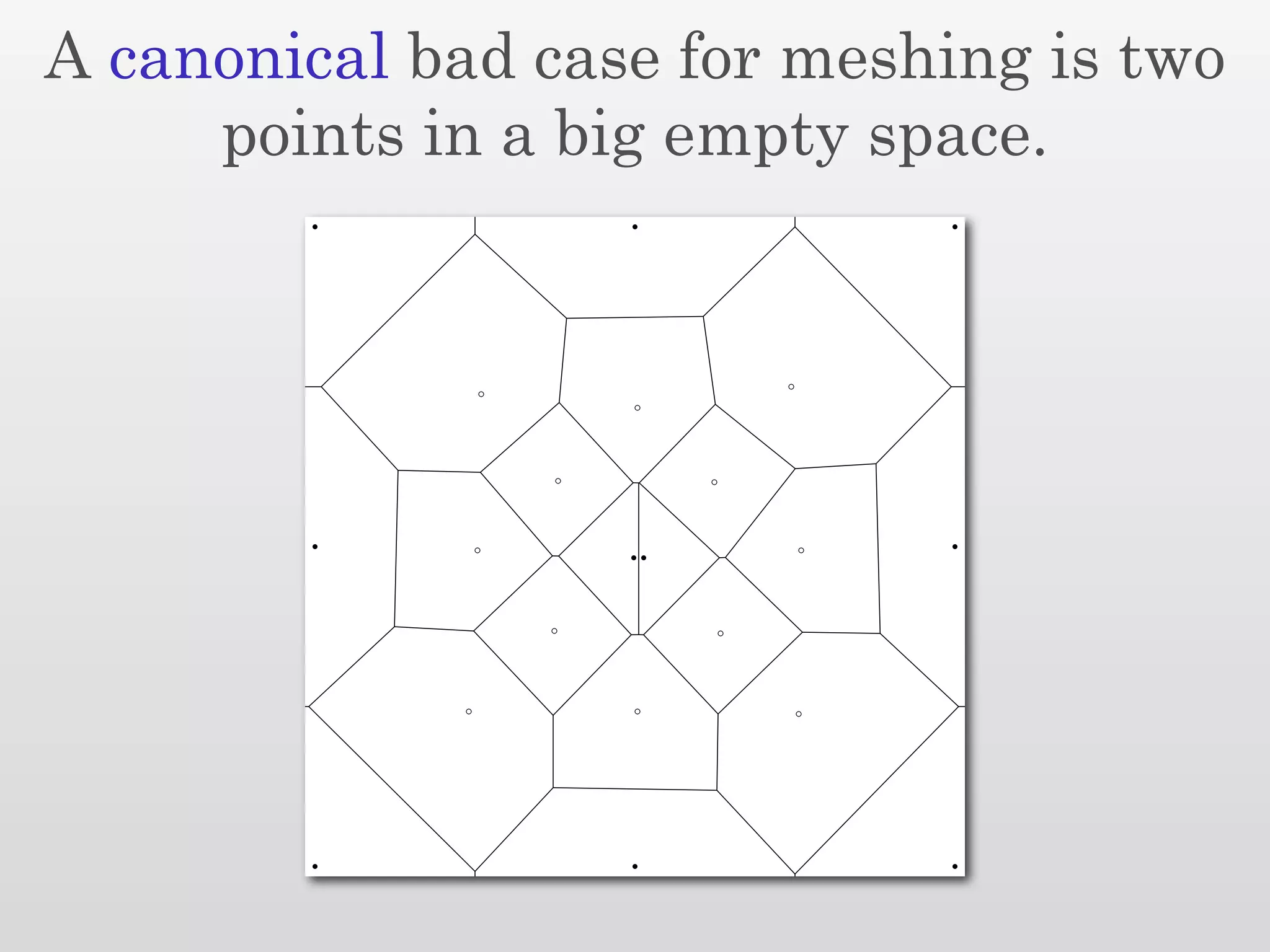
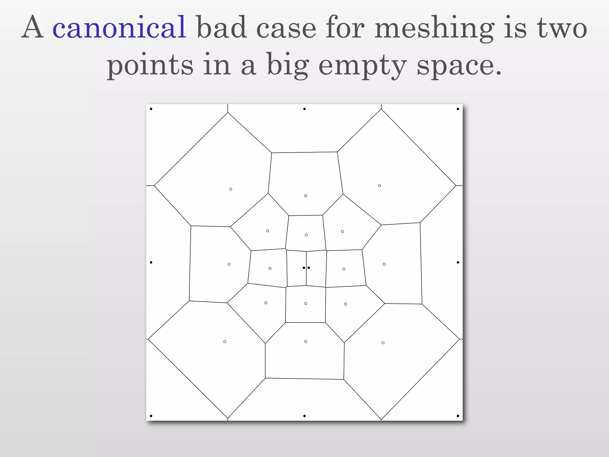
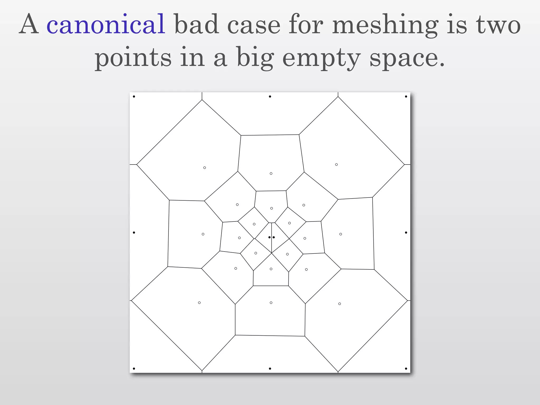
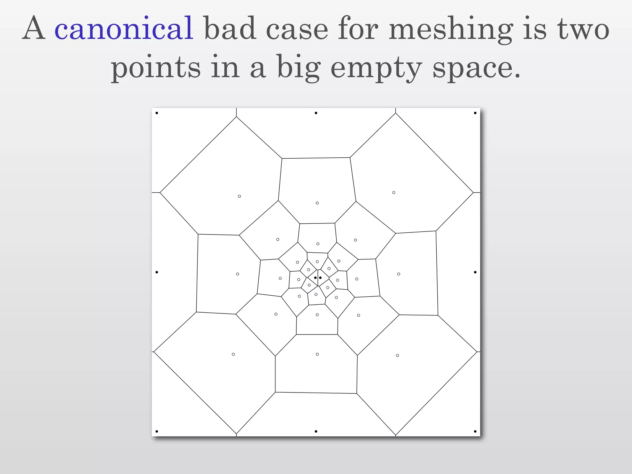
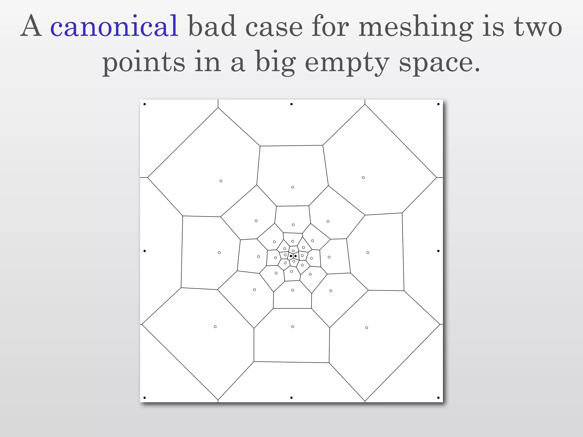
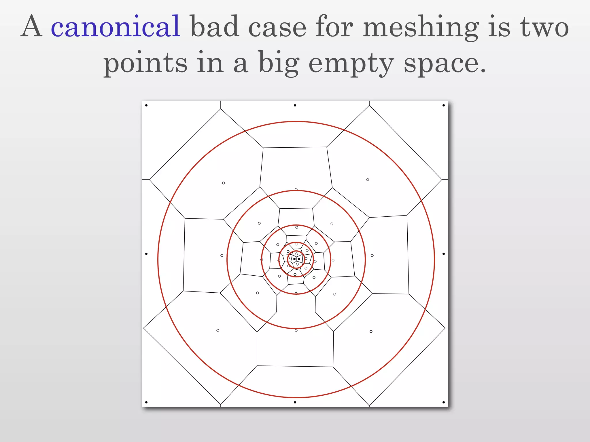
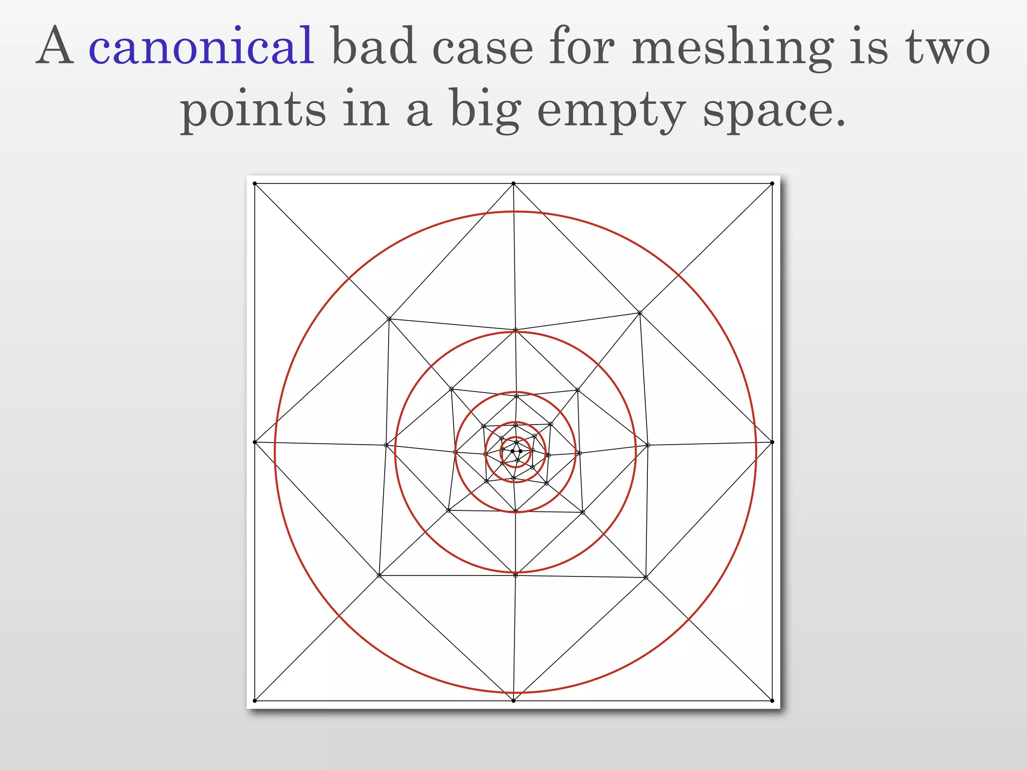


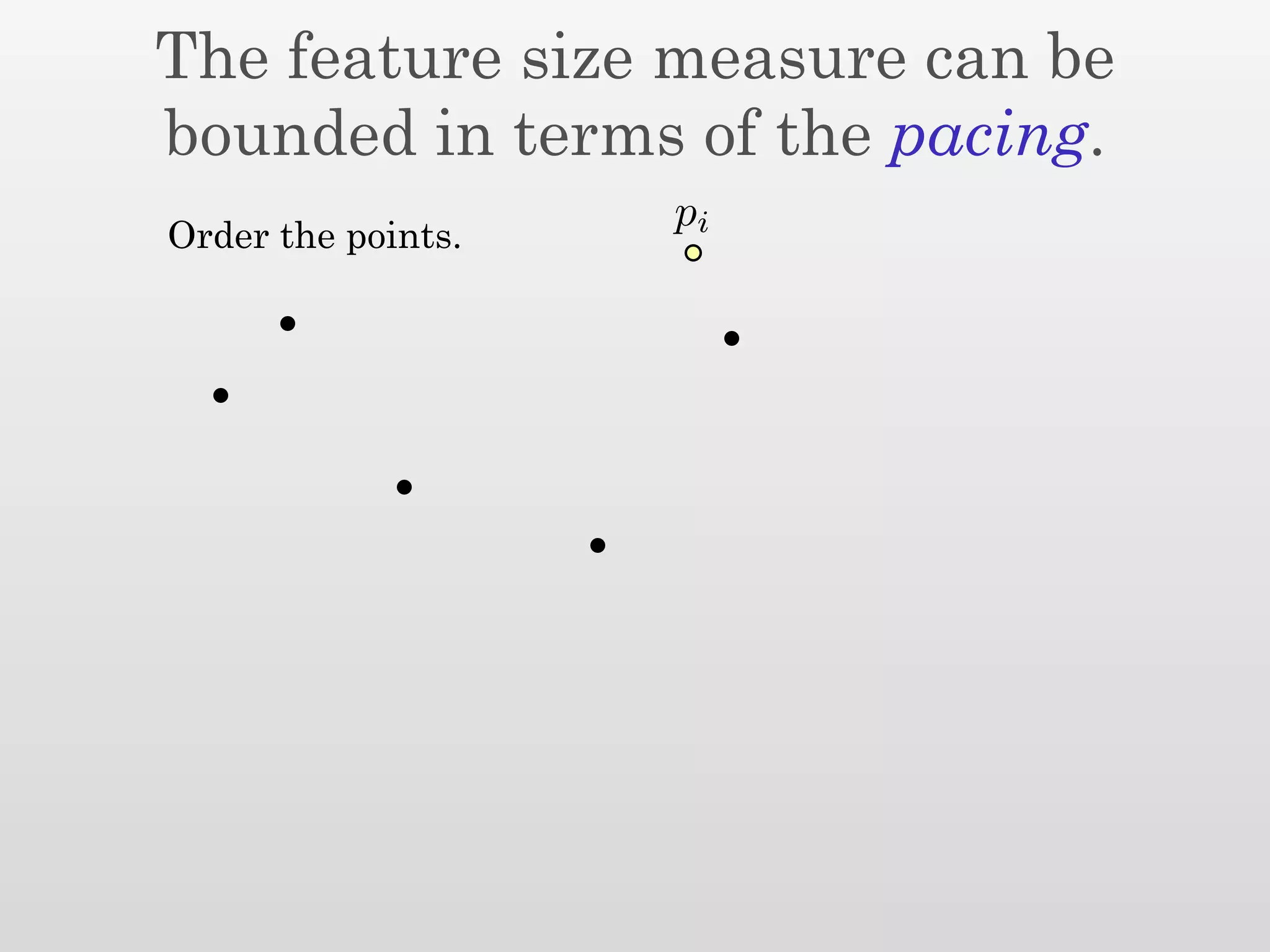
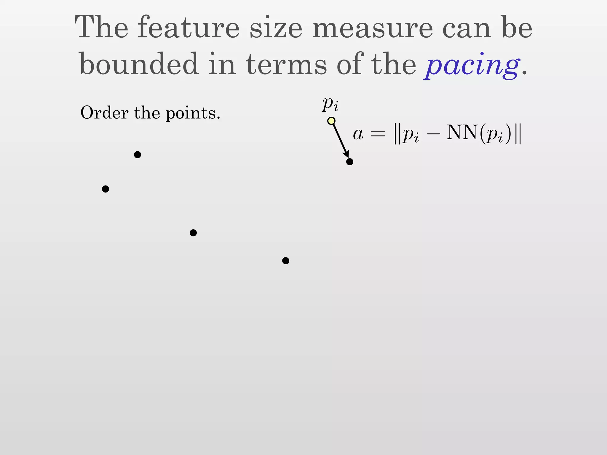
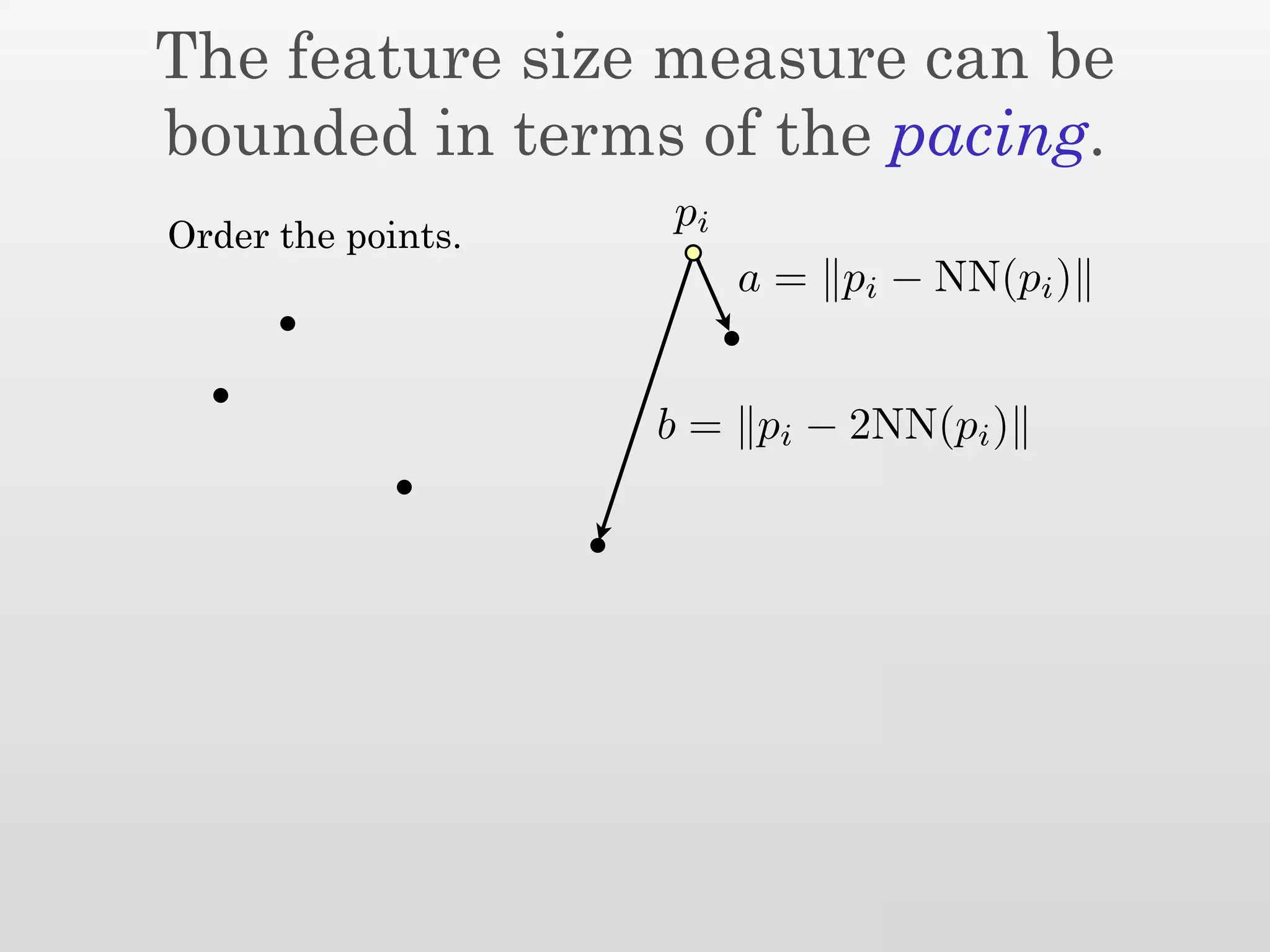
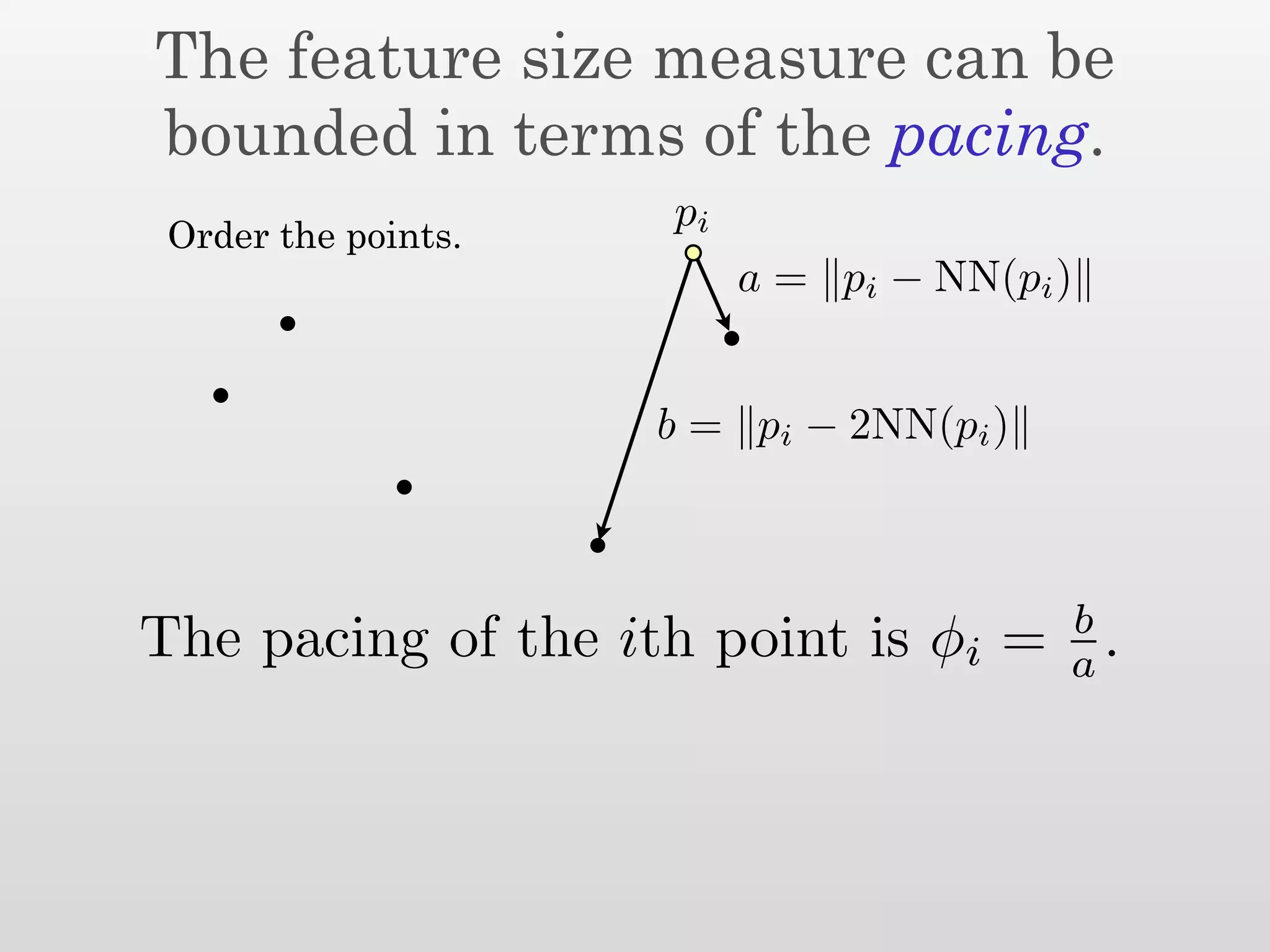
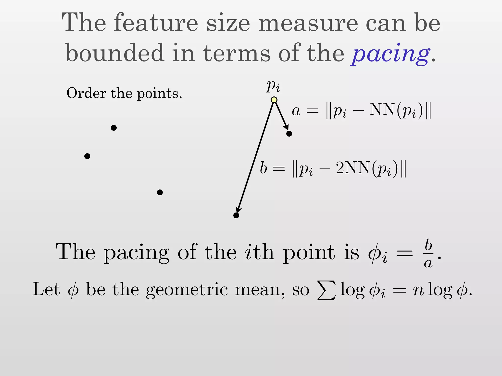
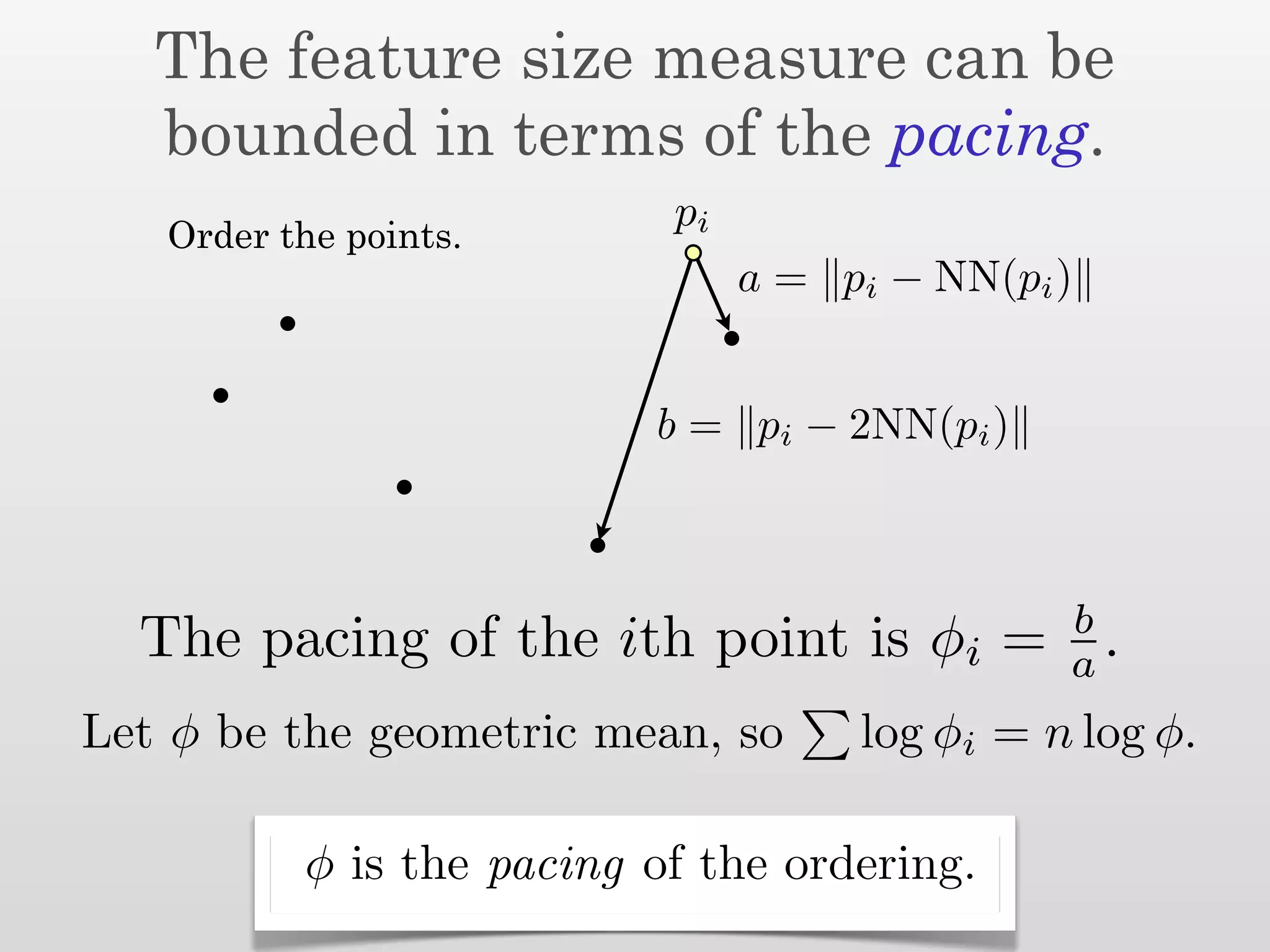
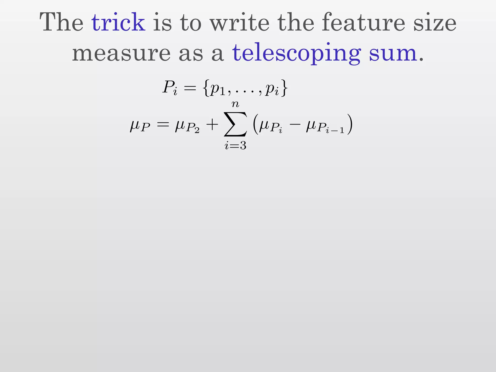
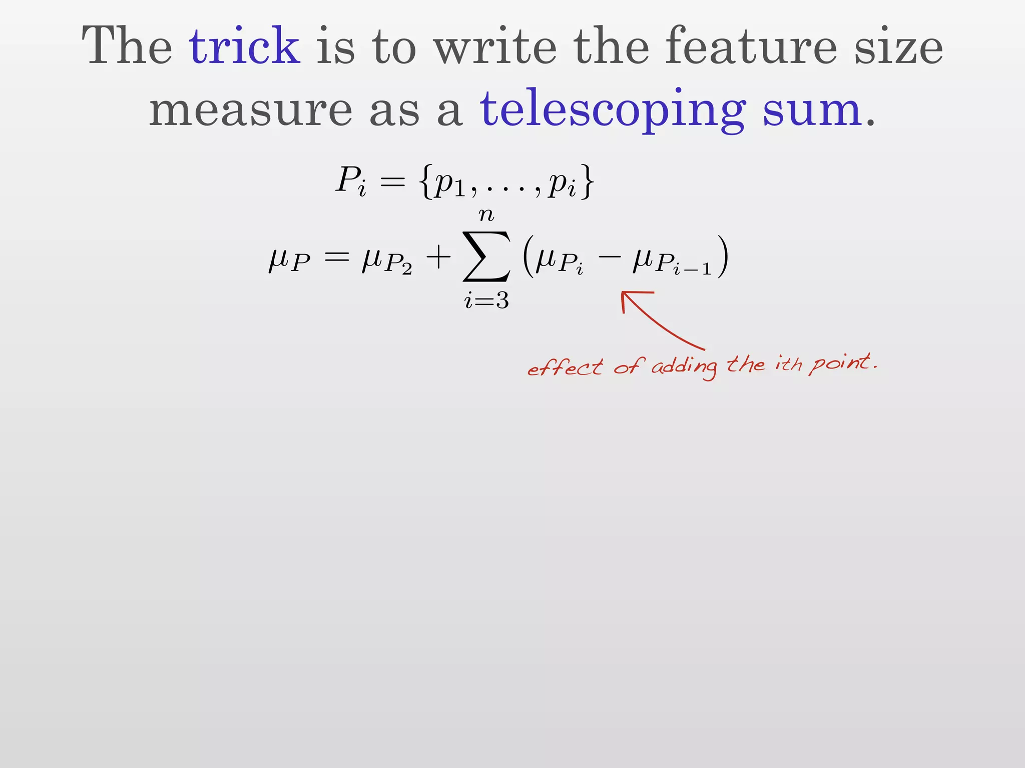
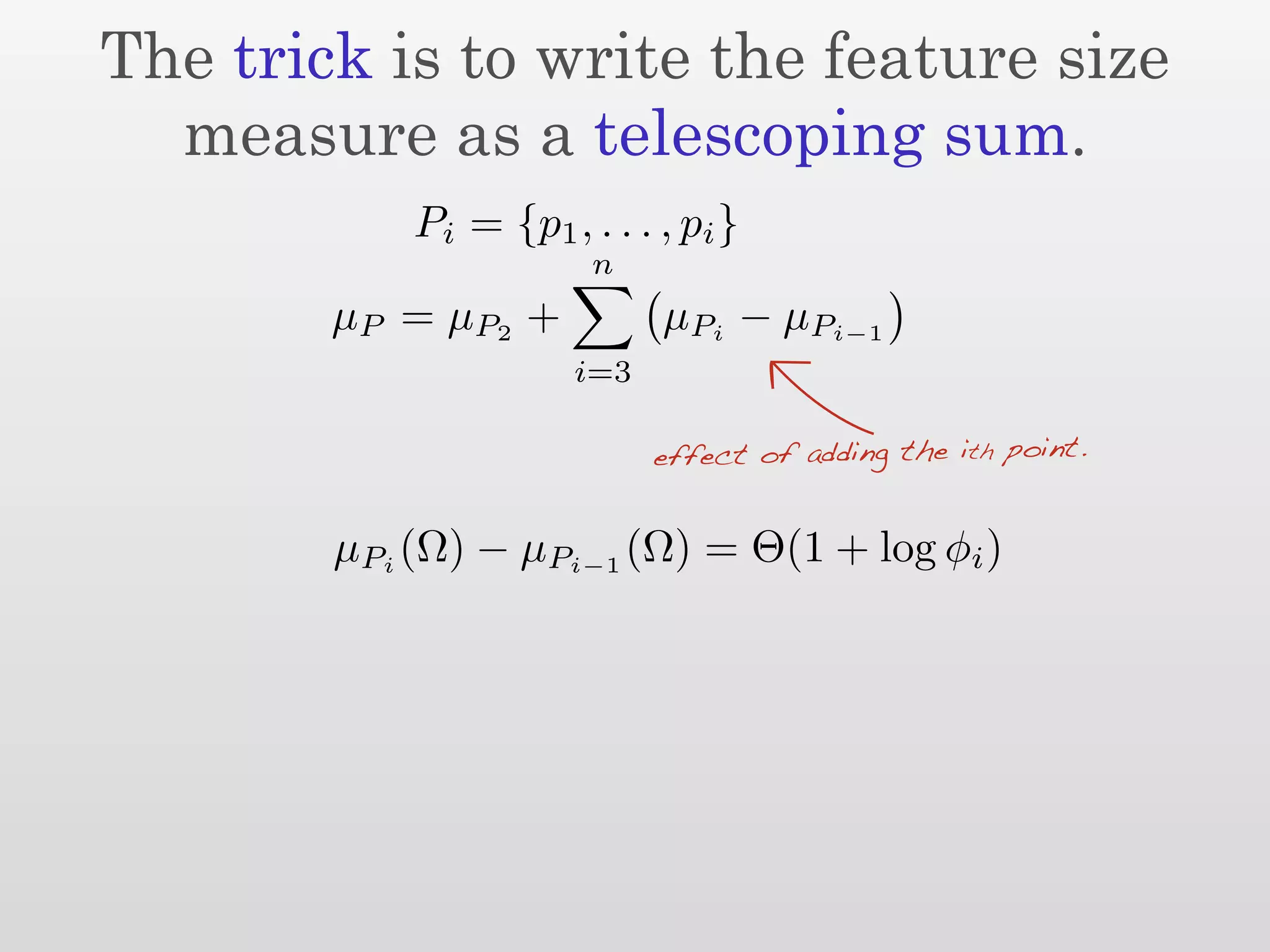
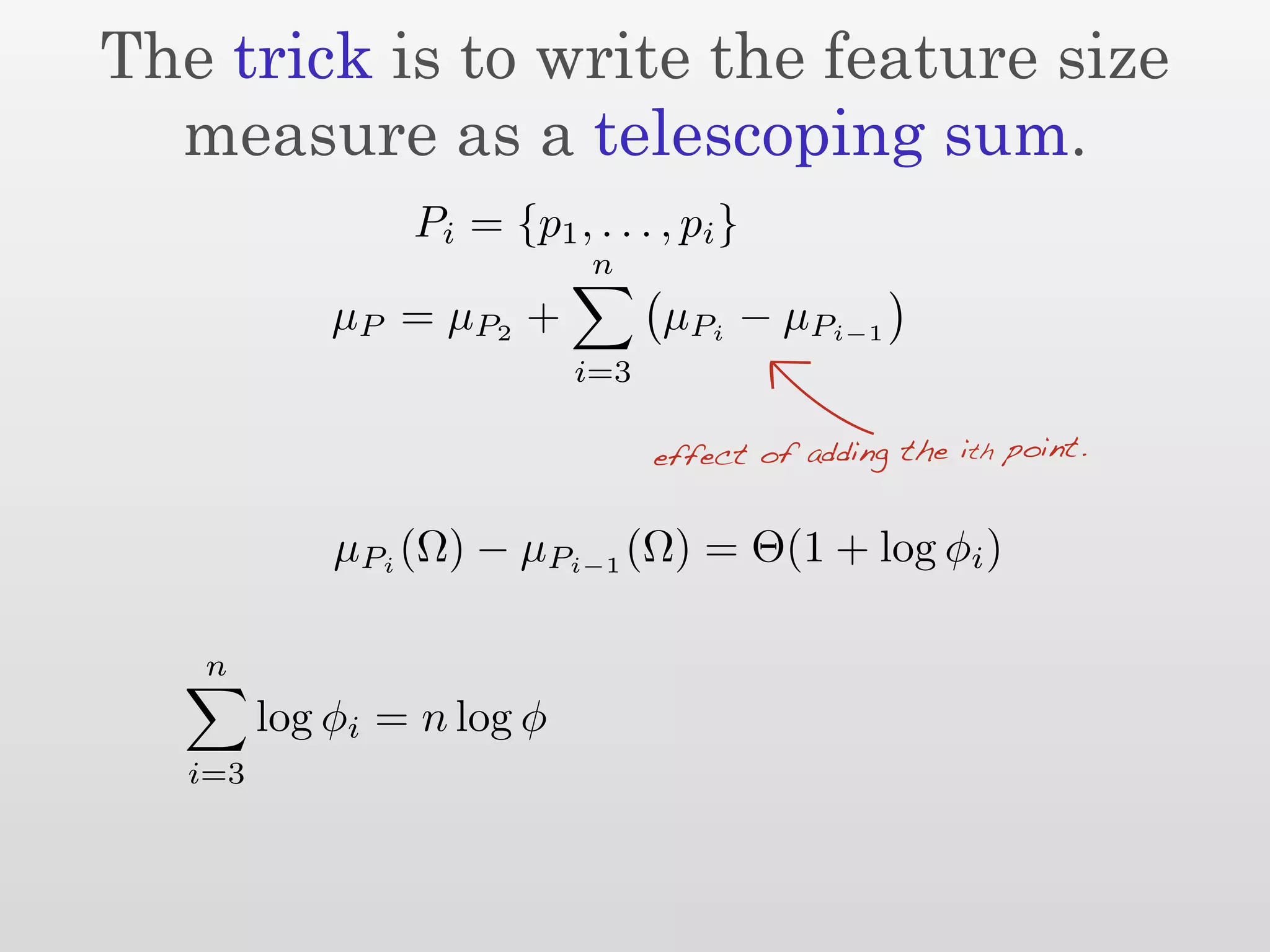
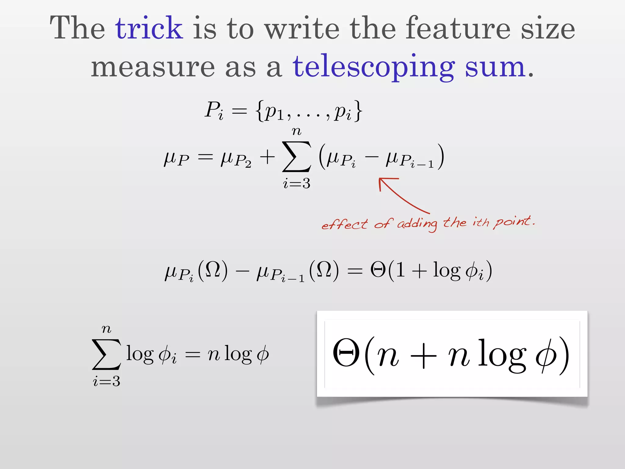
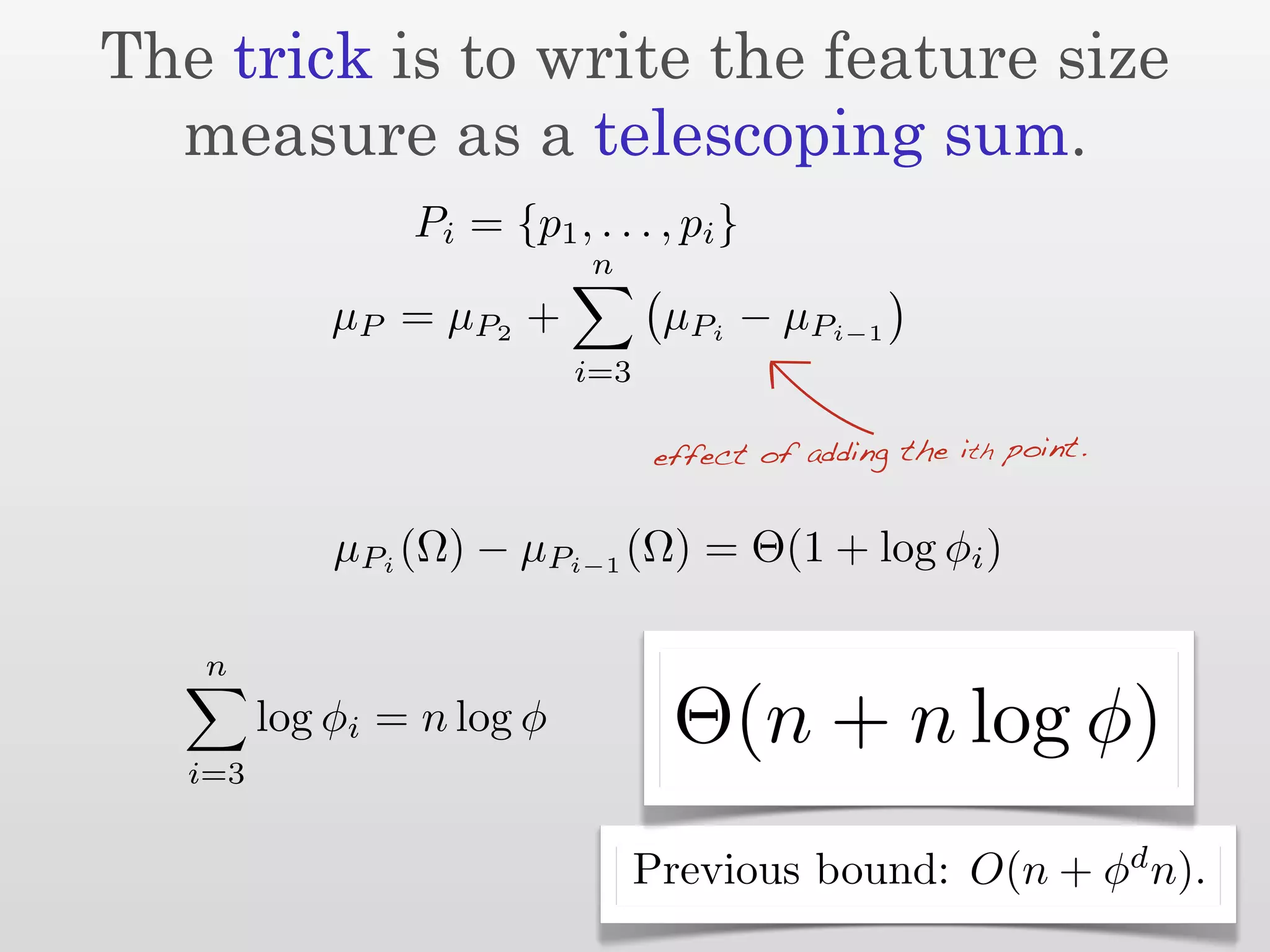


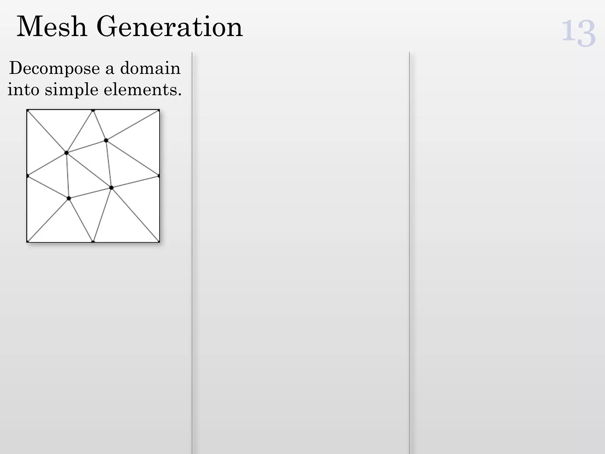
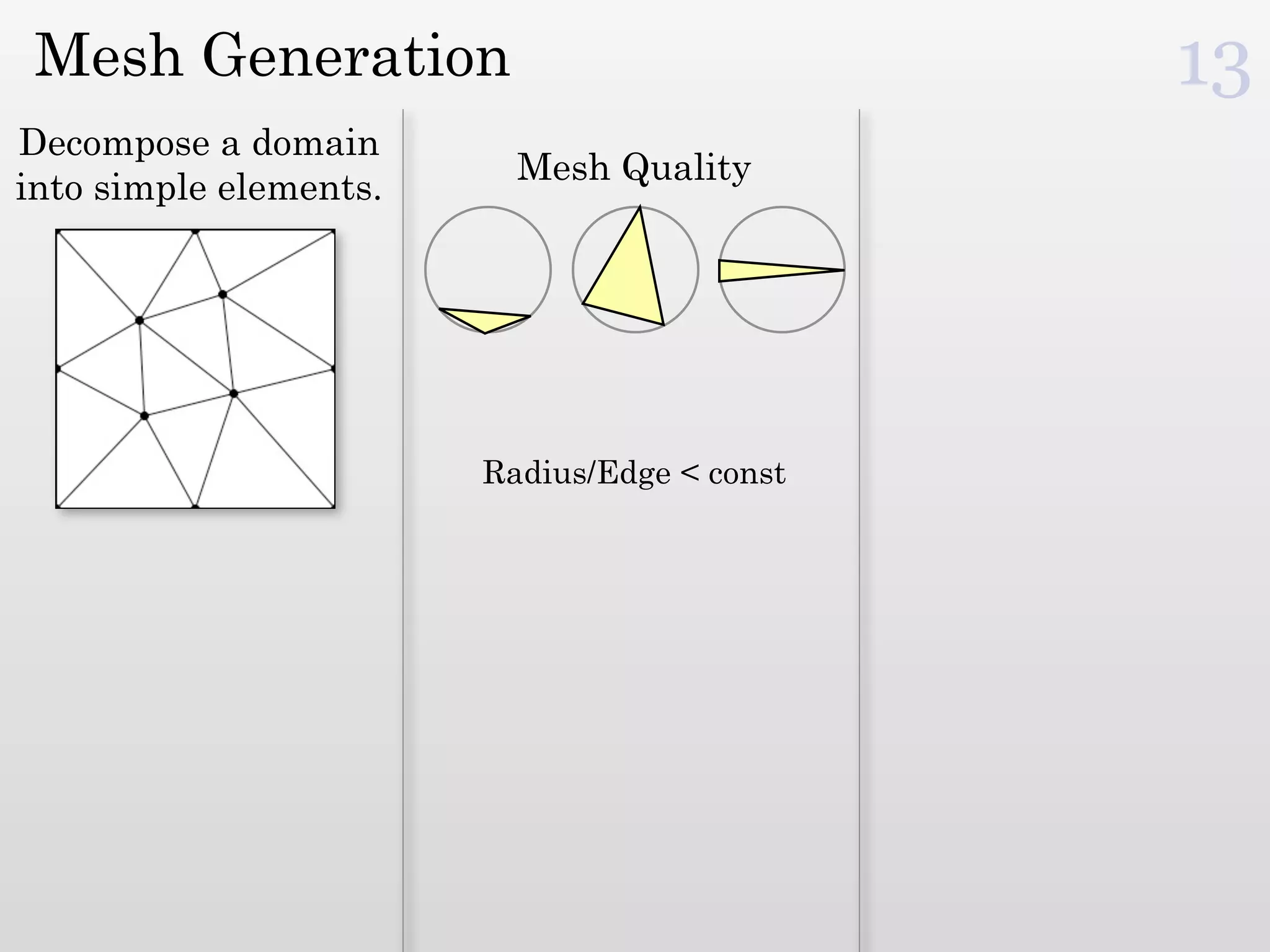
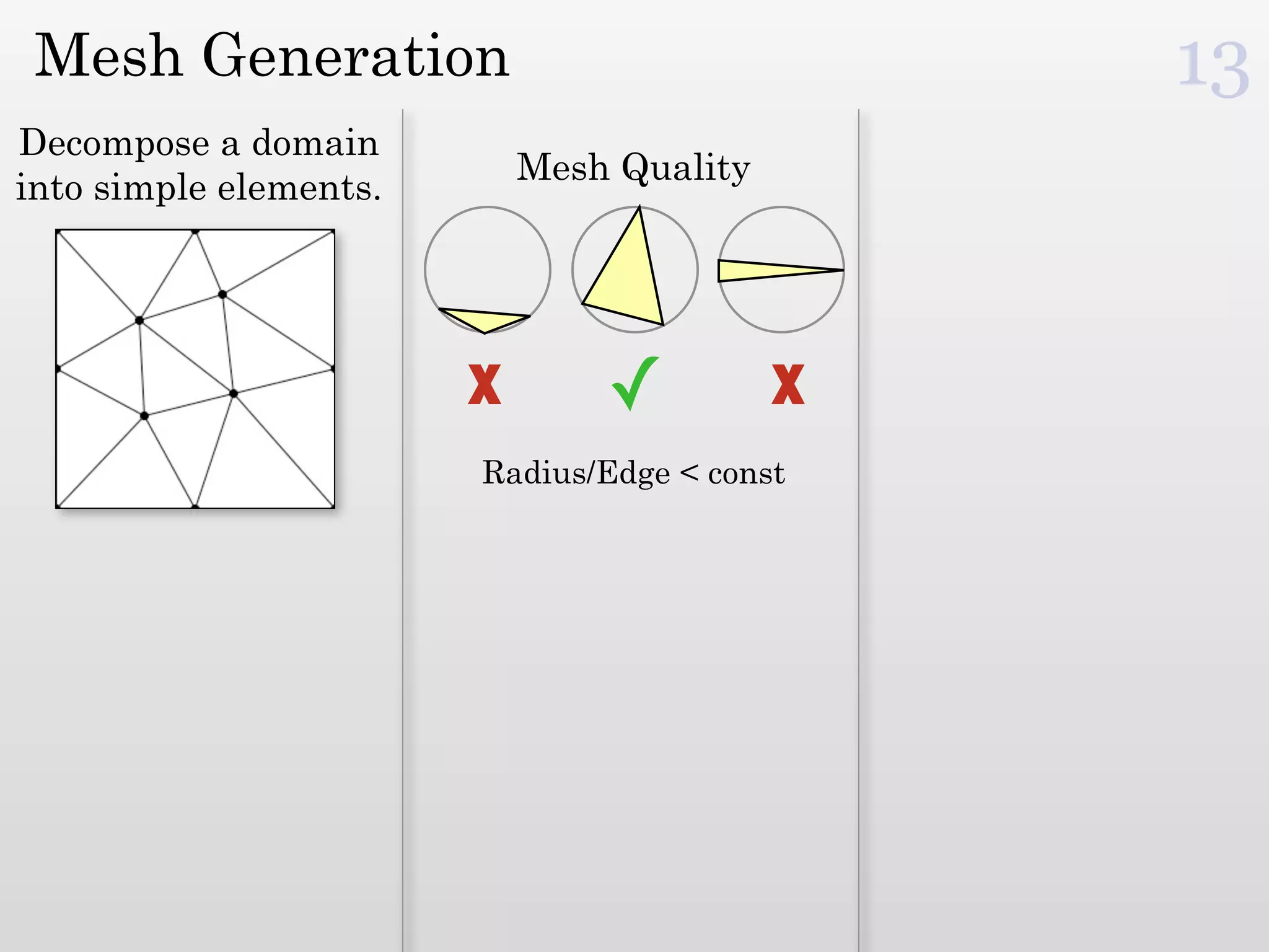
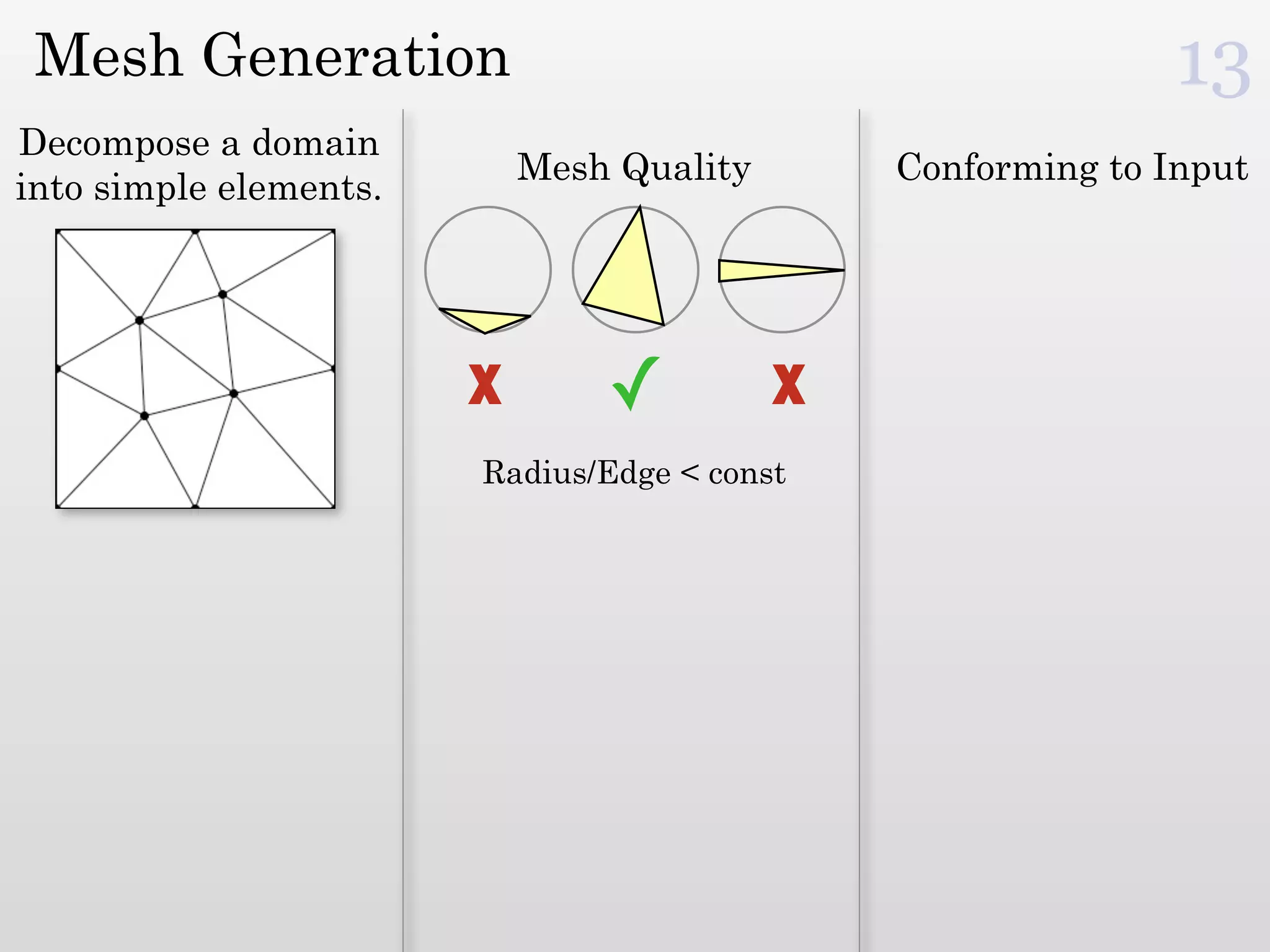
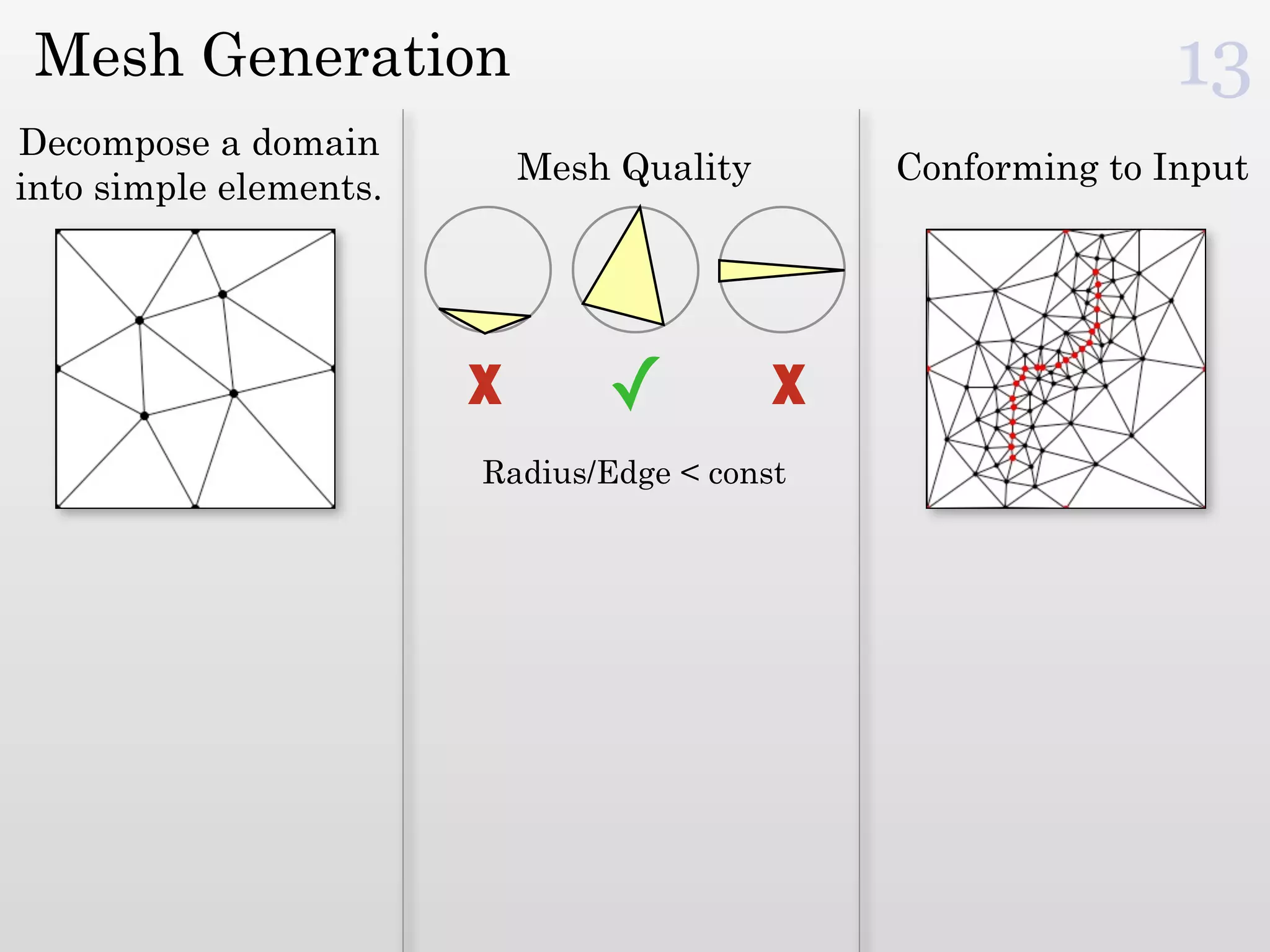
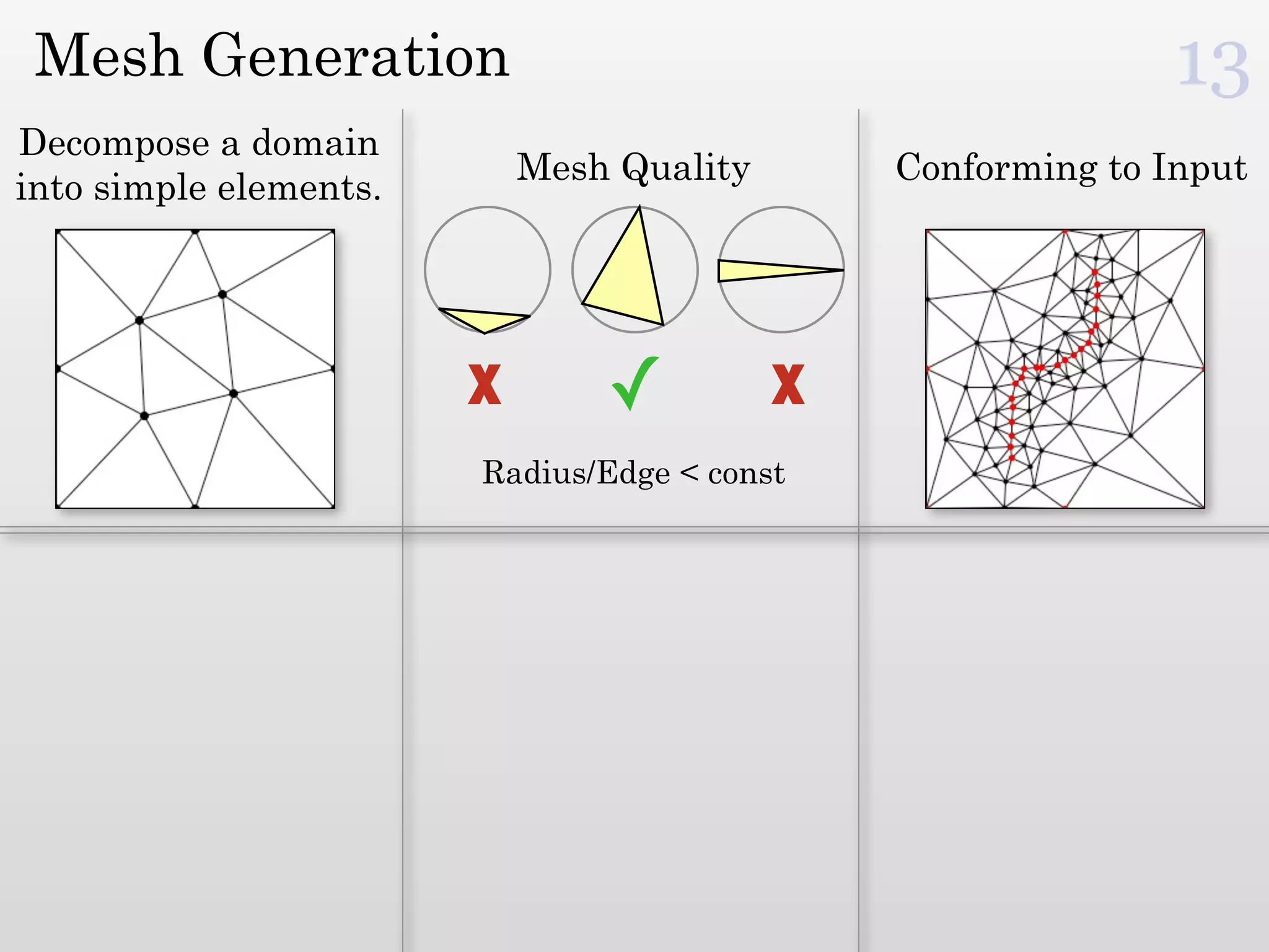
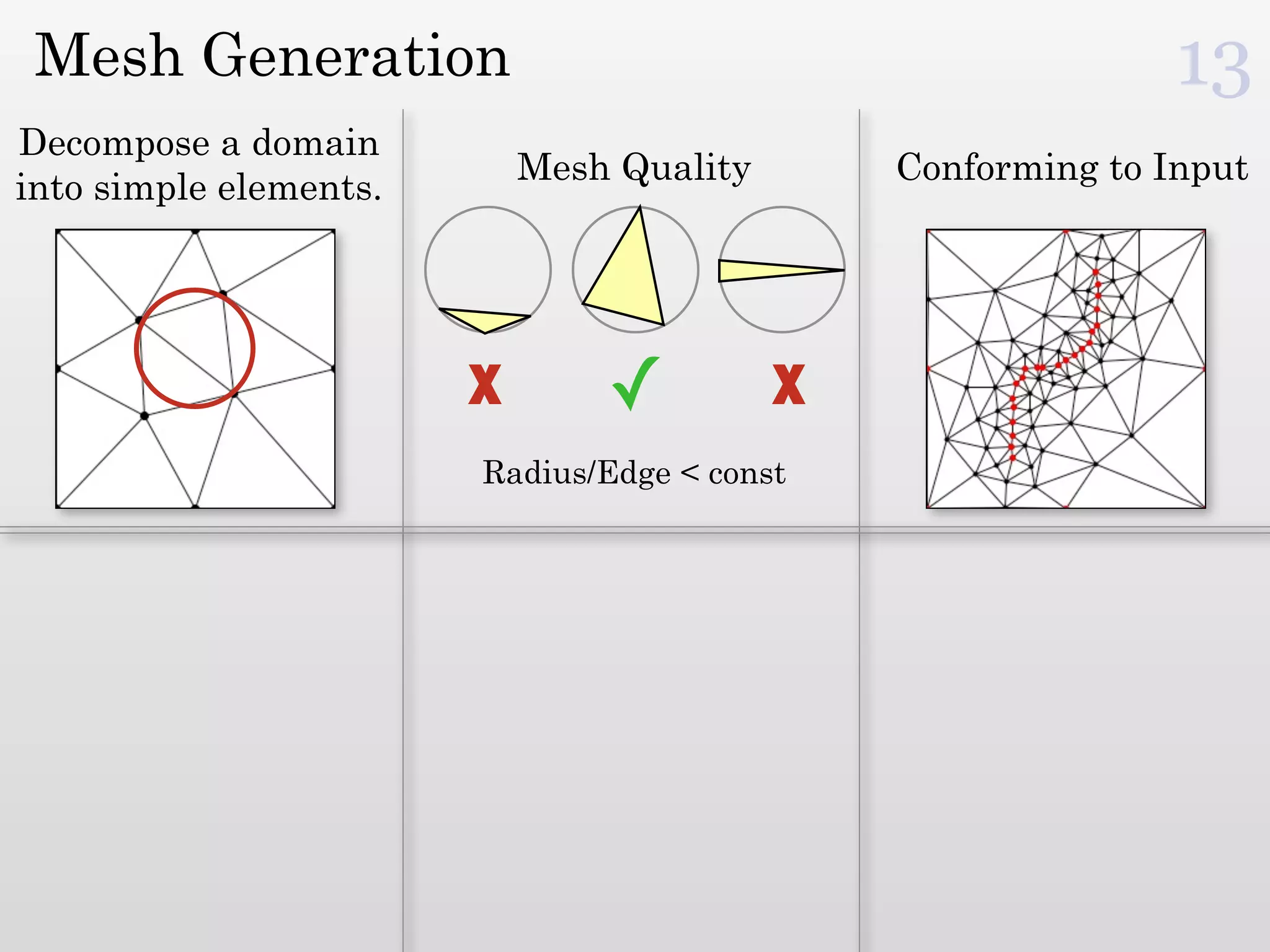
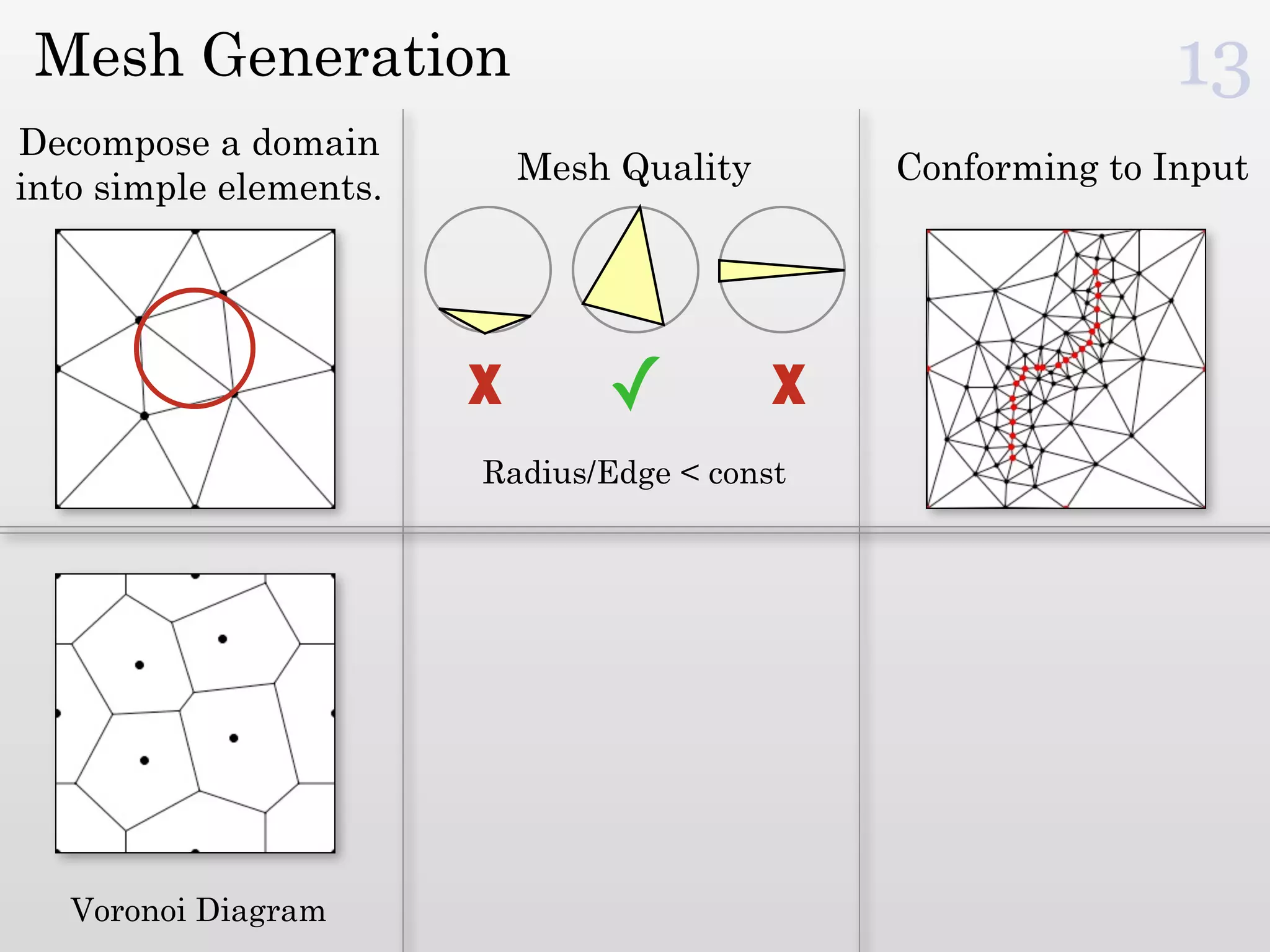
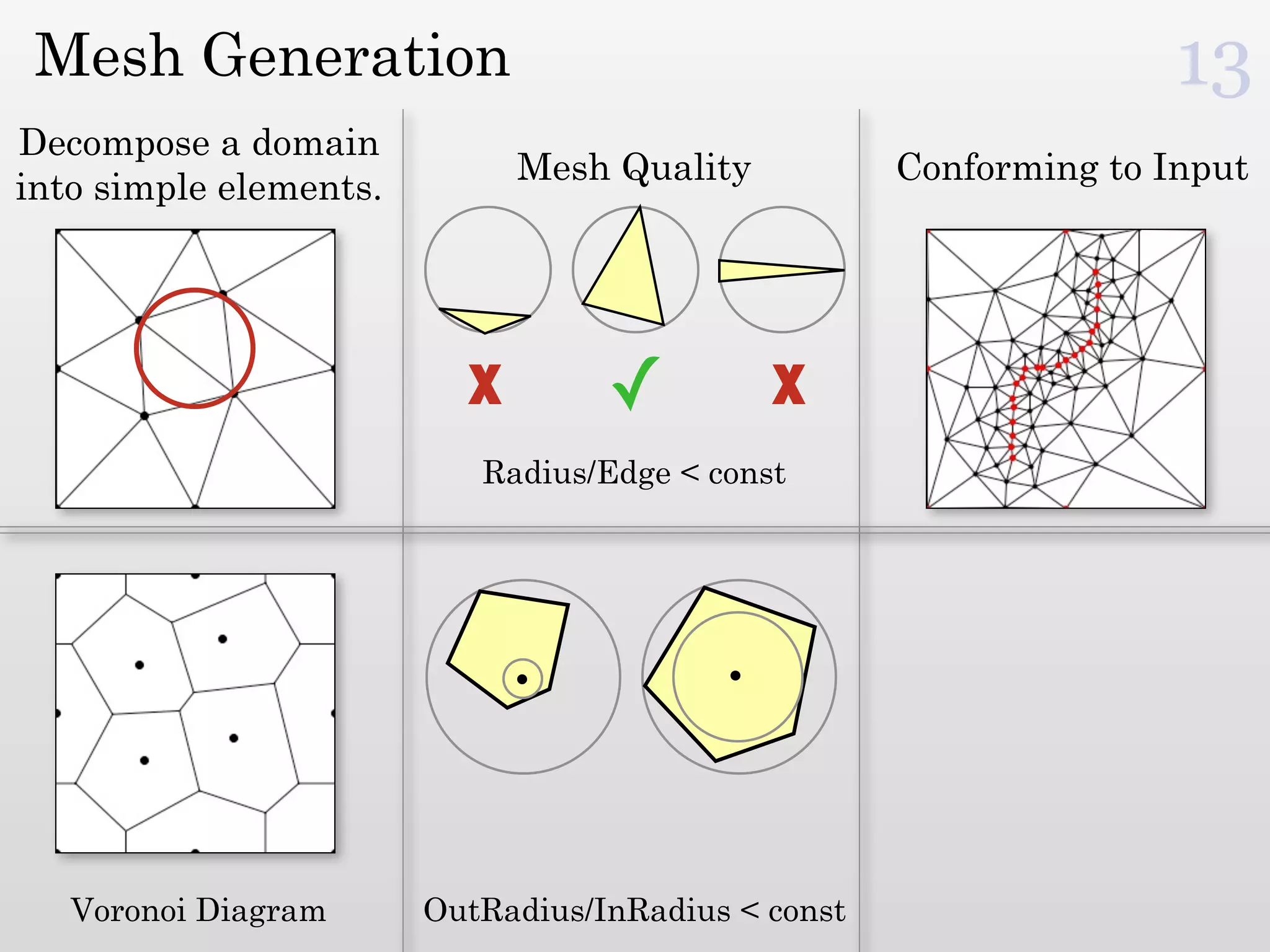
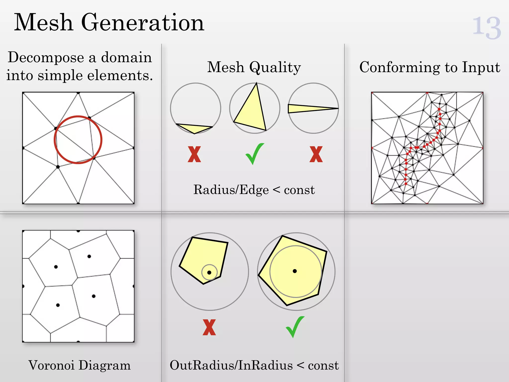
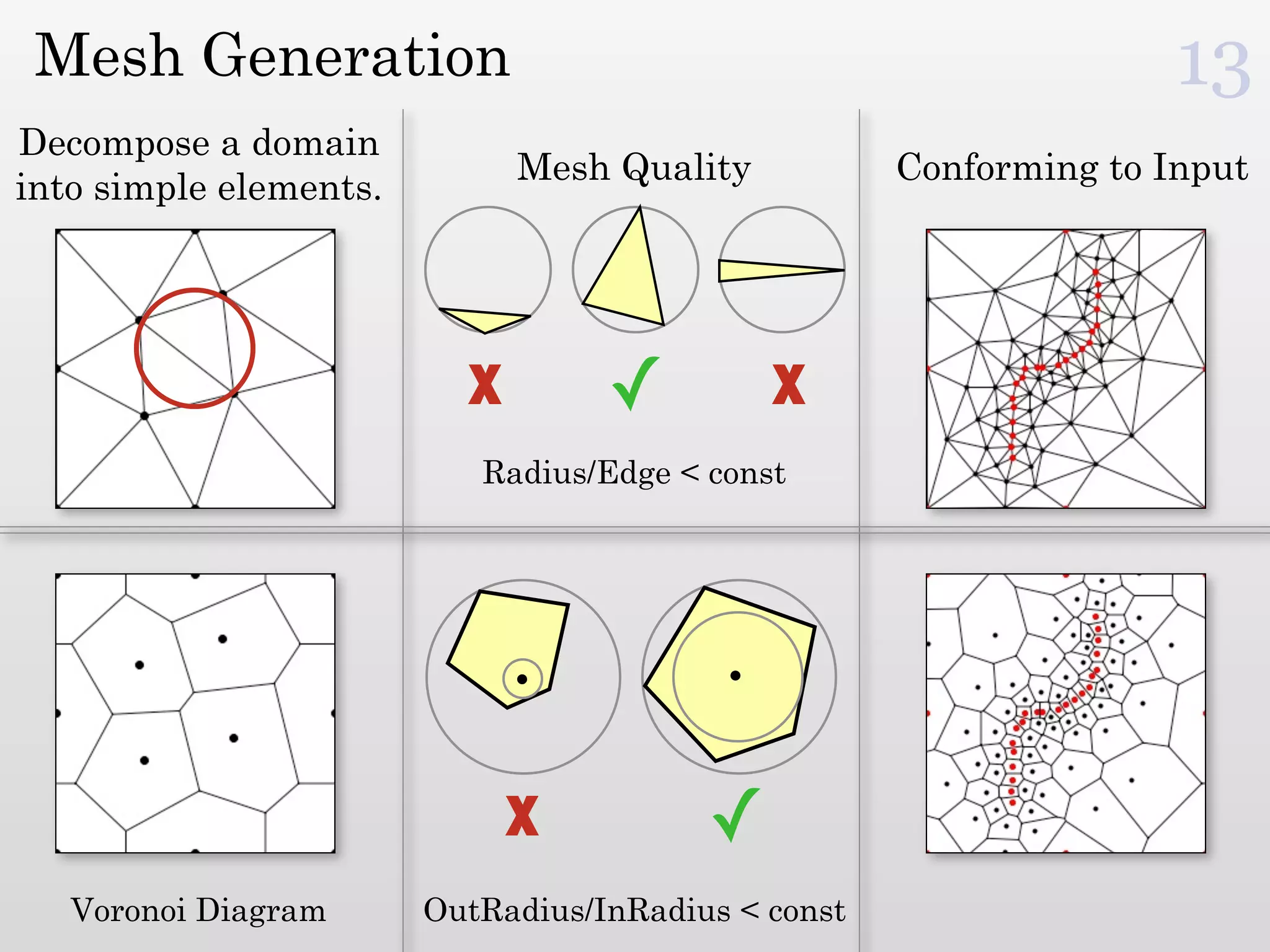
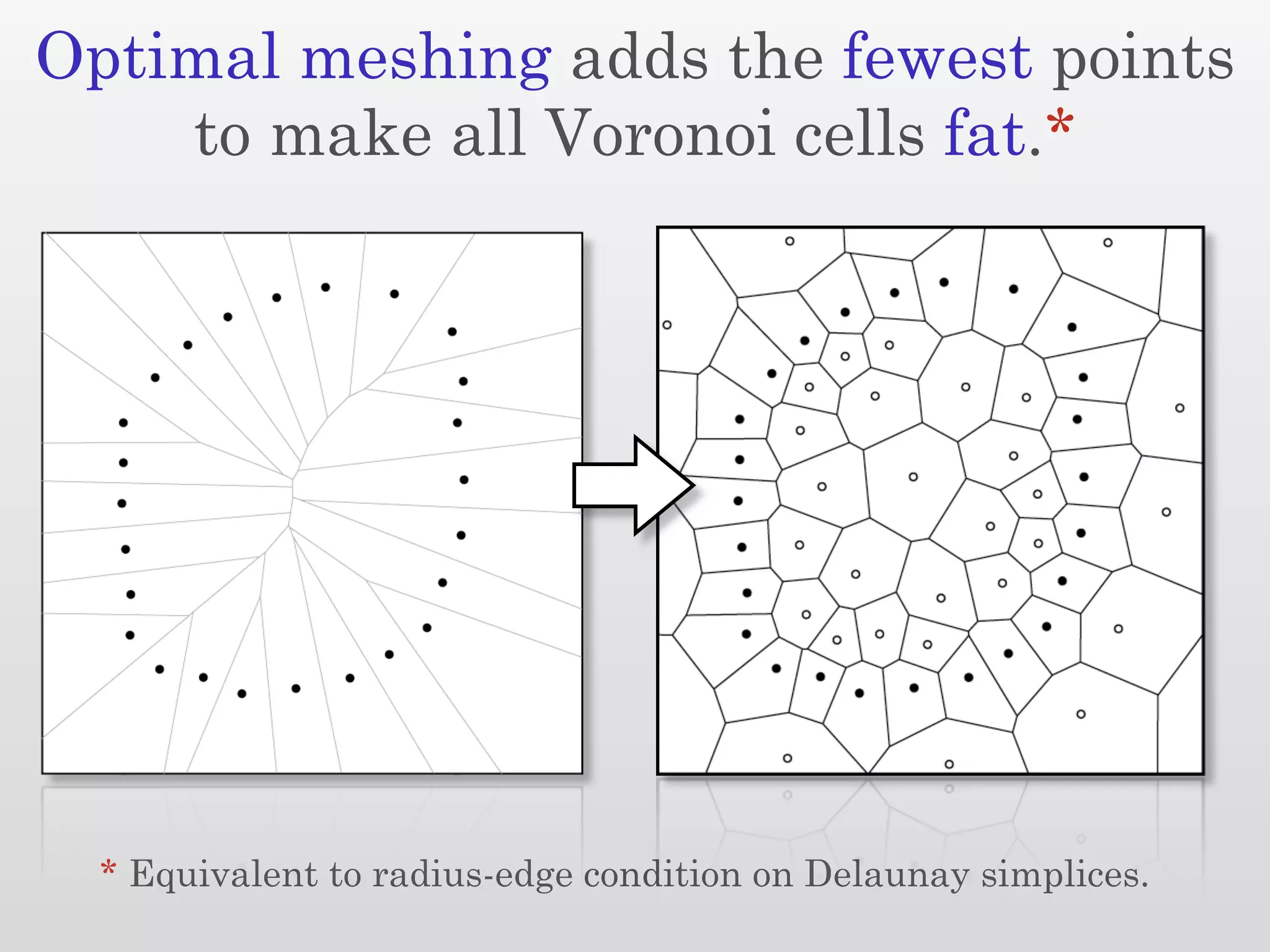
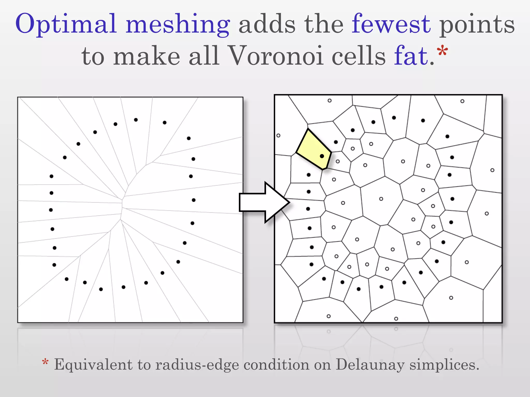
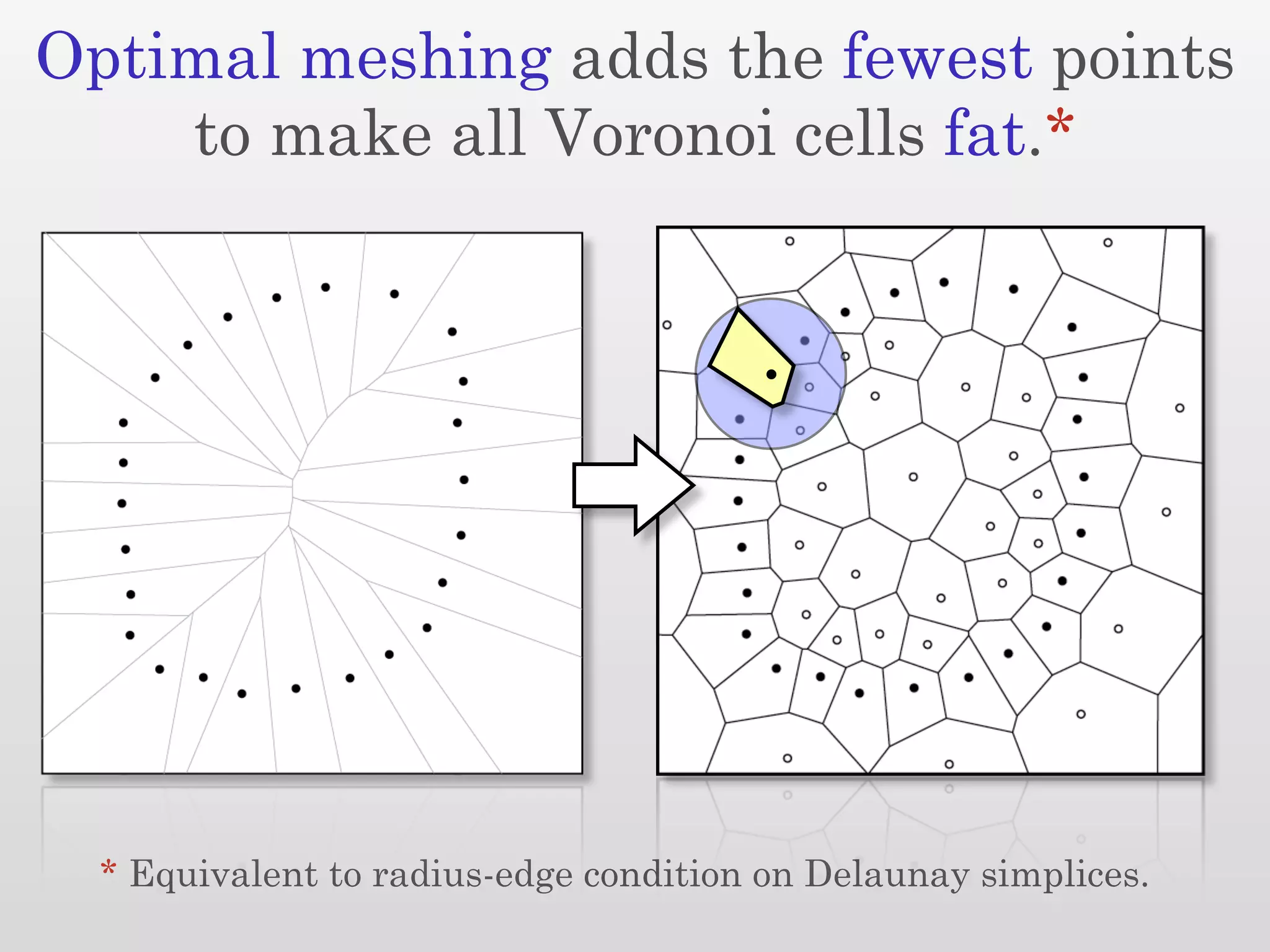
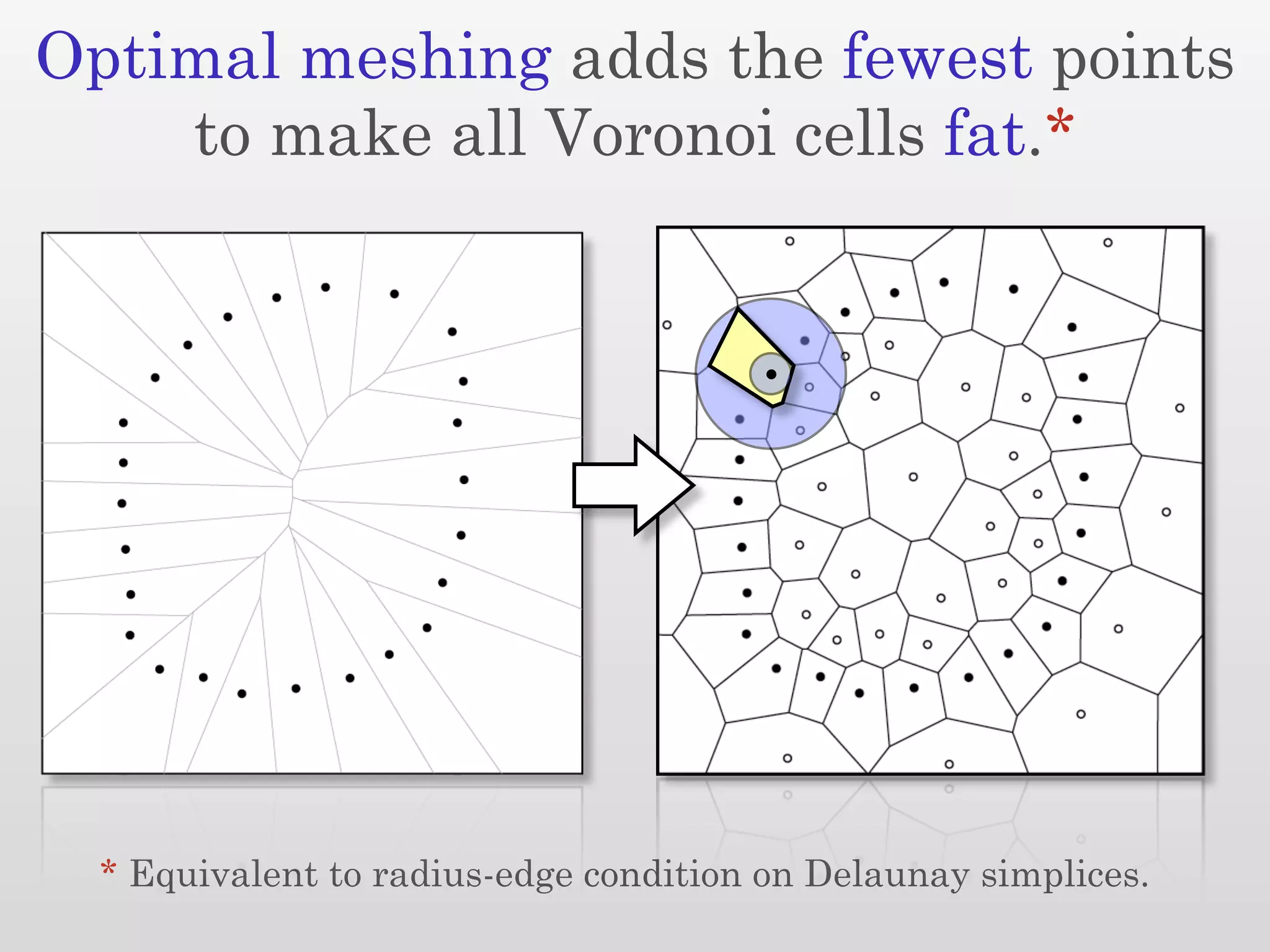
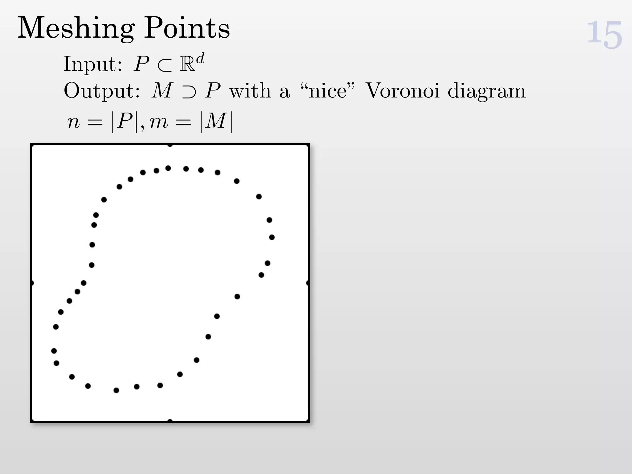
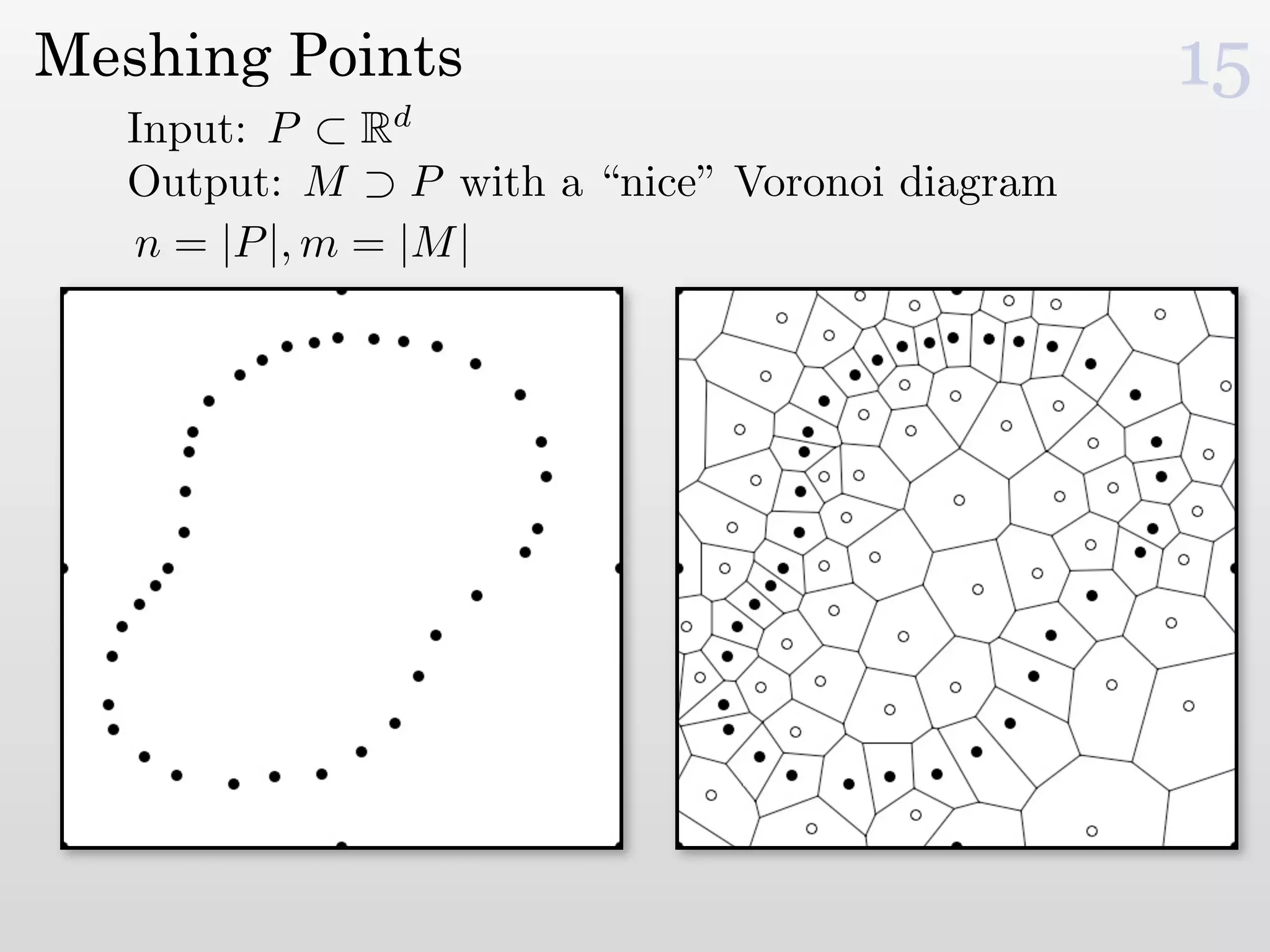
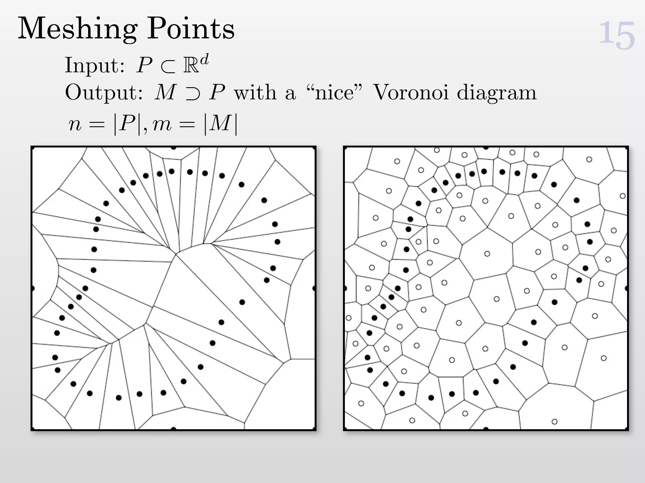
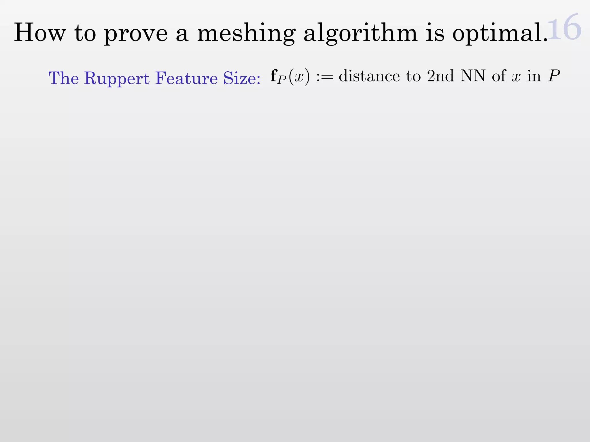

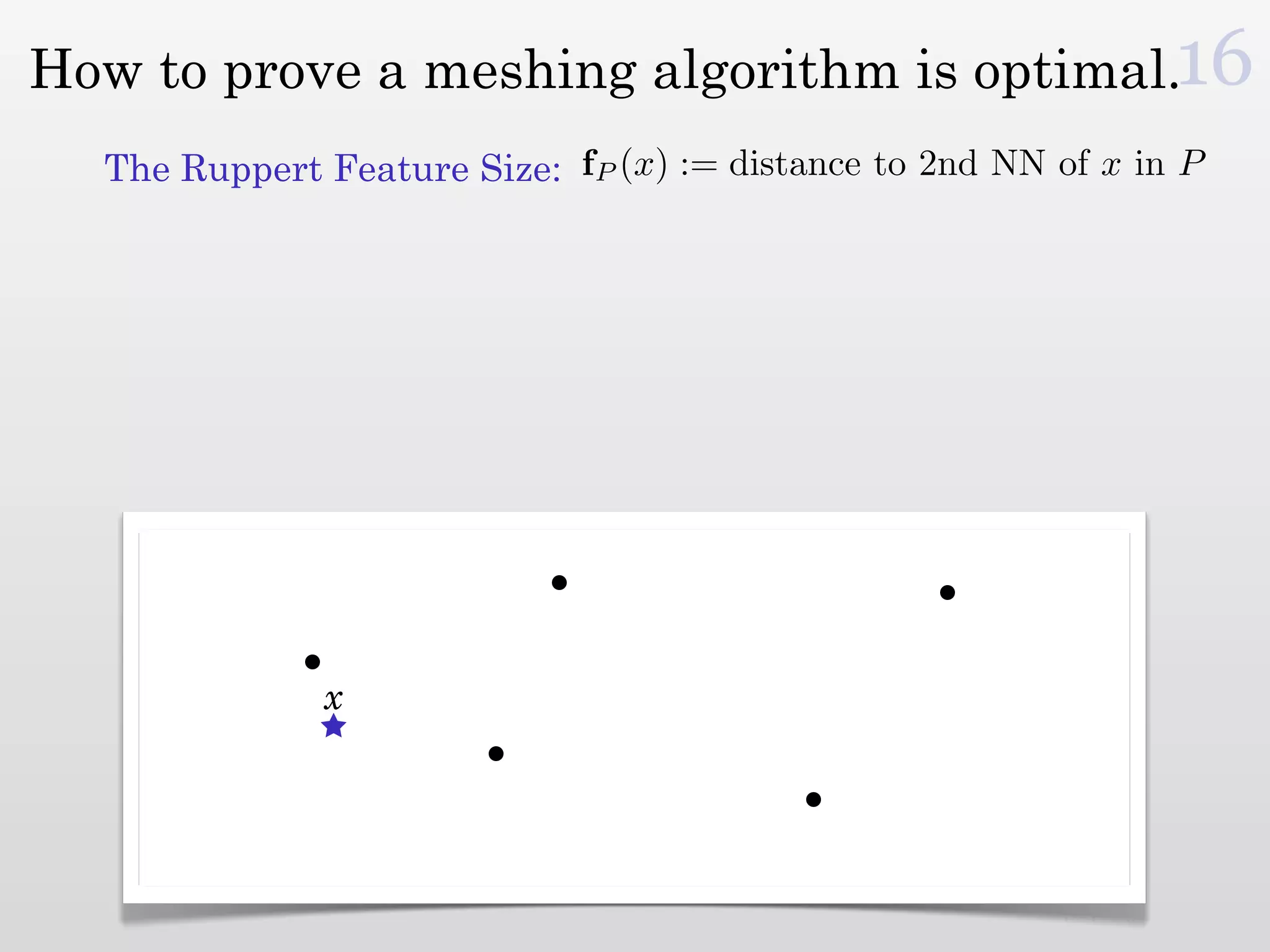

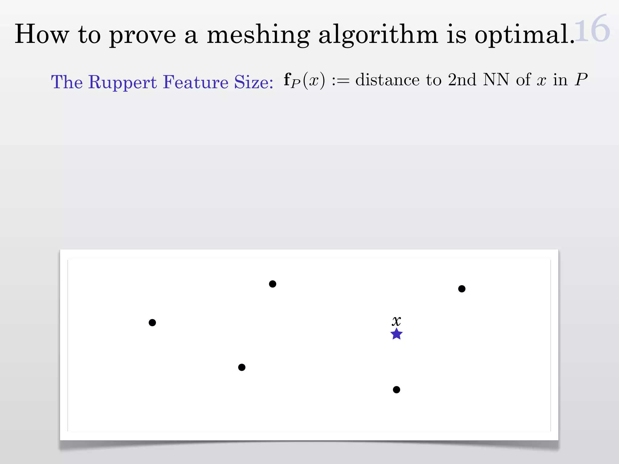
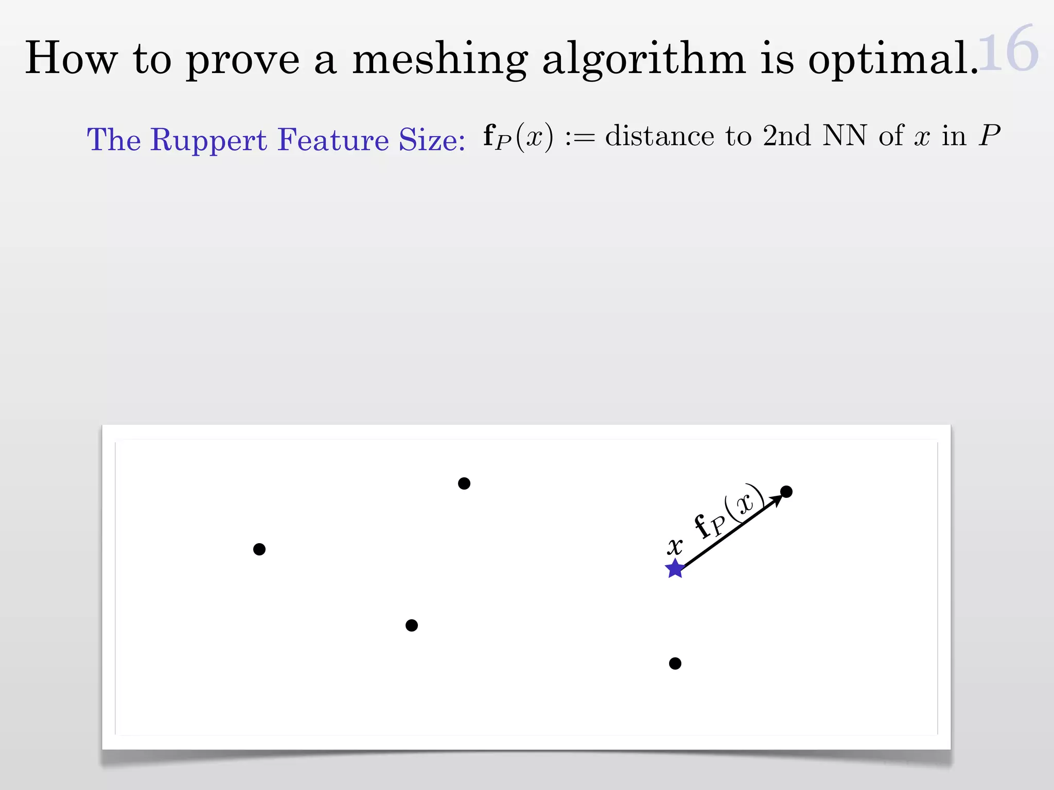
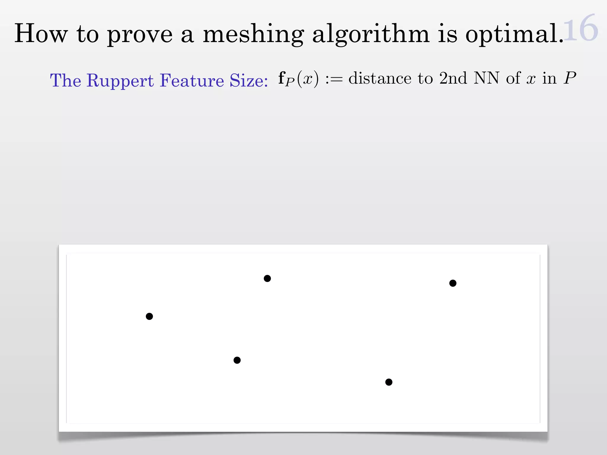
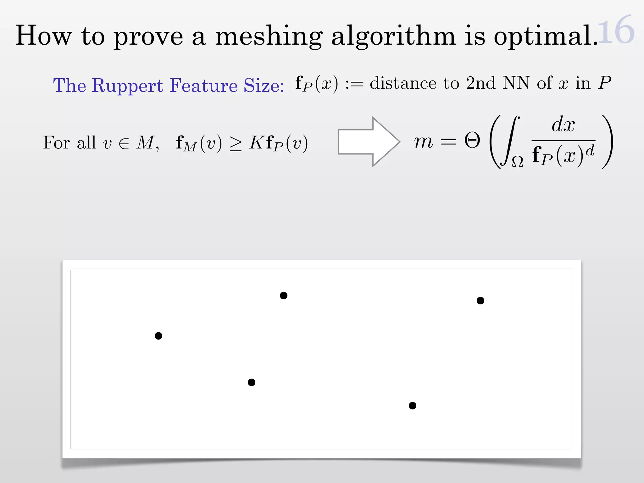
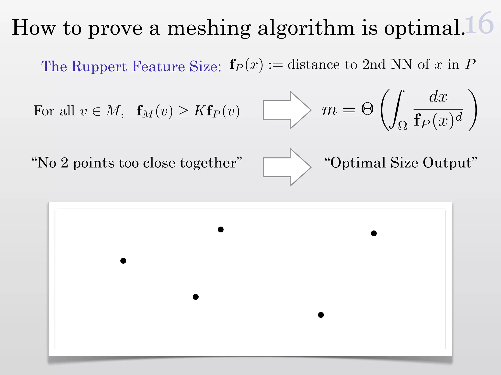
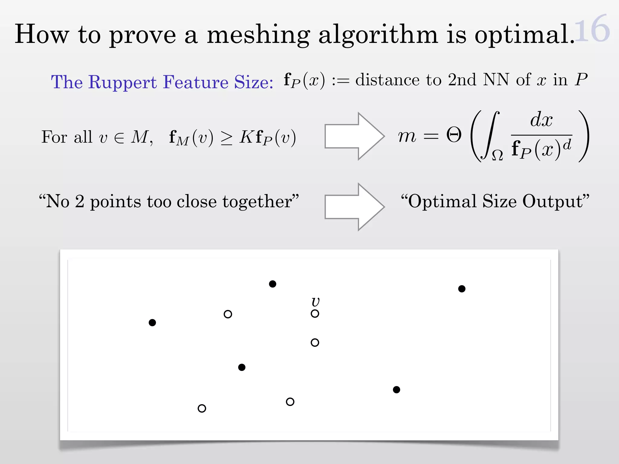
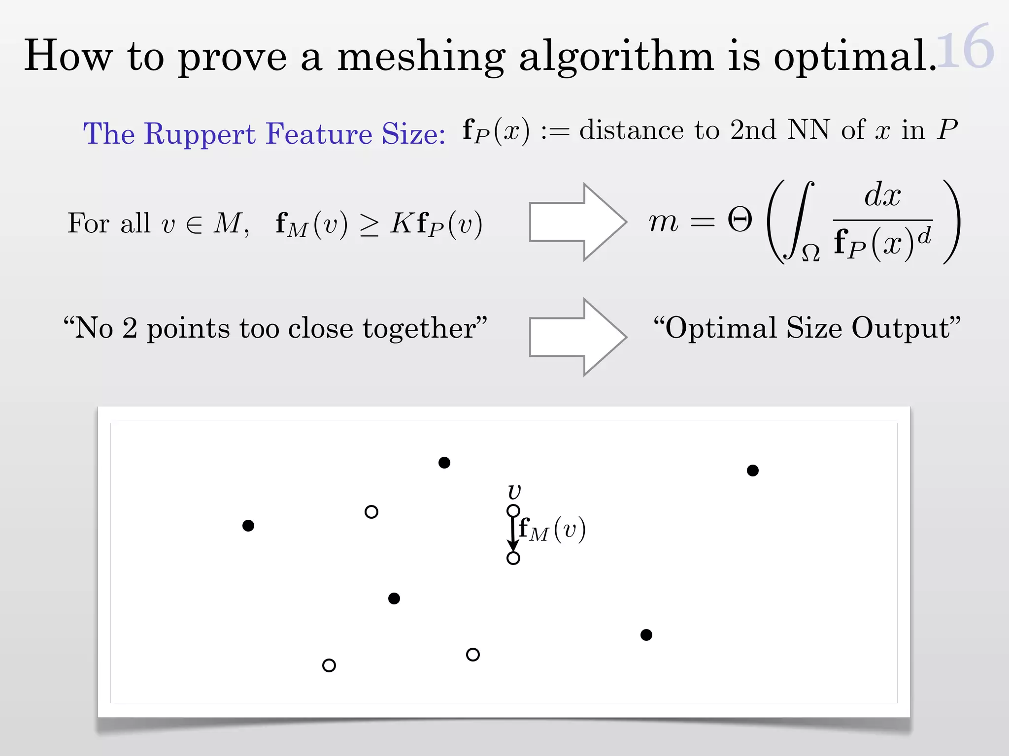
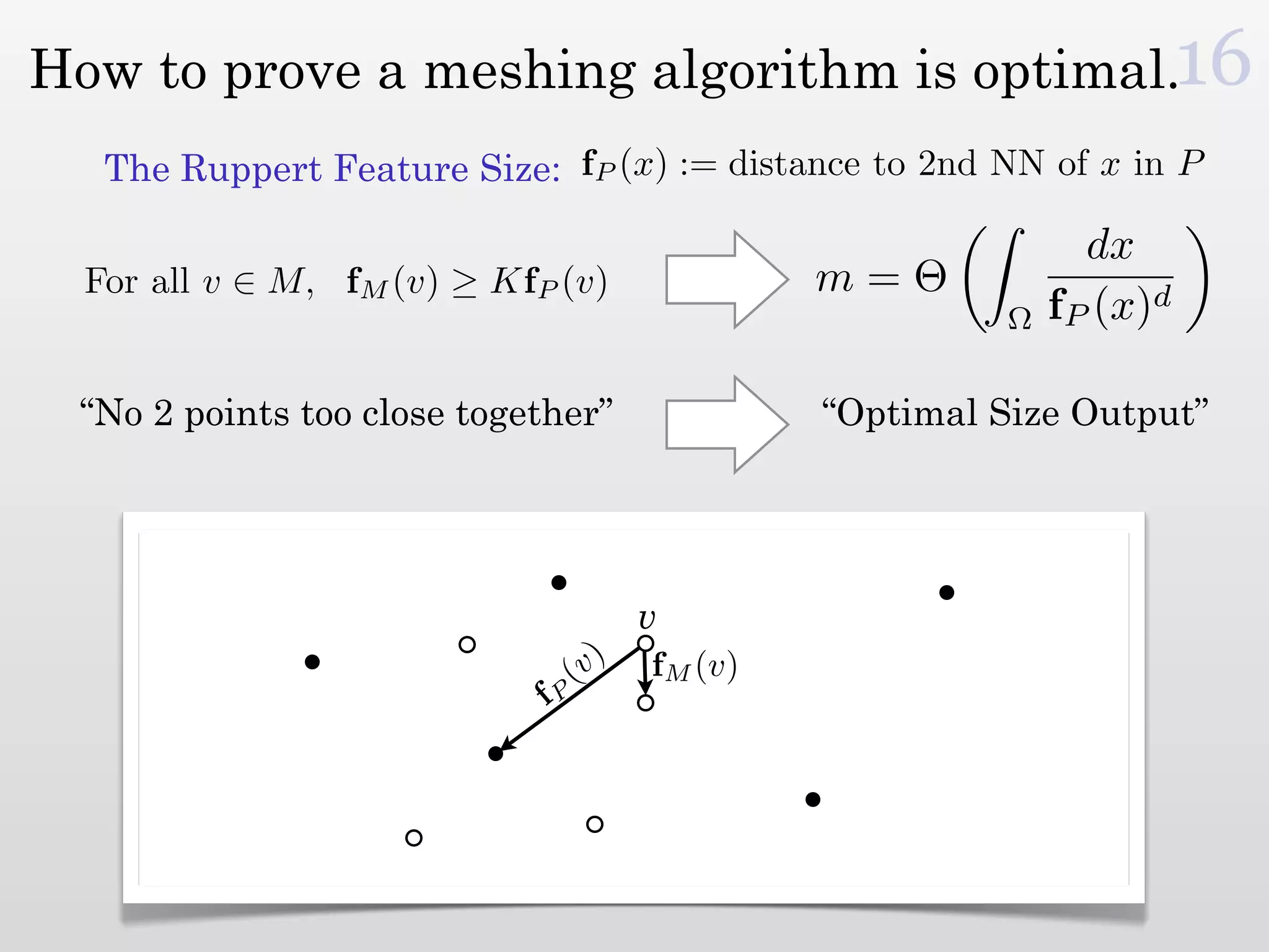

The document discusses mesh generation, which involves decomposing a domain into simple elements like triangles or tetrahedra. An optimal mesh has good element quality, conforms to the input domain, and uses the minimum number of points needed to make all Voronoi cells sufficiently "fat" or well-shaped according to metrics like radius-edge ratios. The talk presents analysis showing that the optimal mesh size is determined by the "feature size measure" of the input points, which involves the distance to each point's second nearest neighbor.