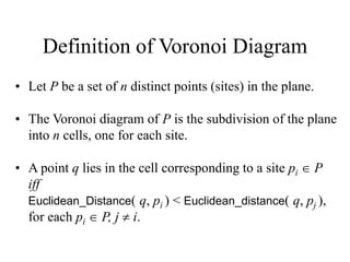
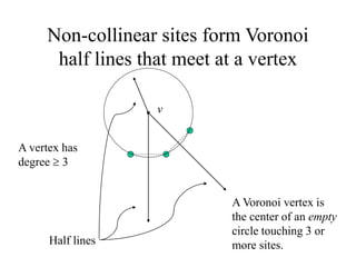
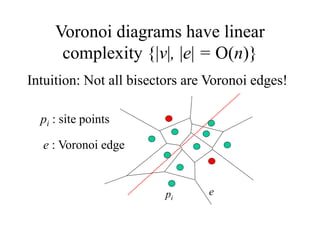
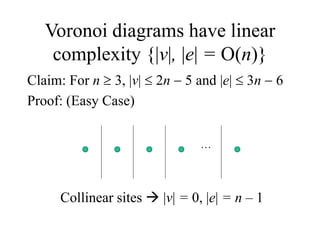
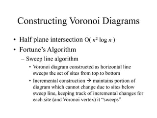
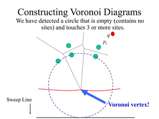
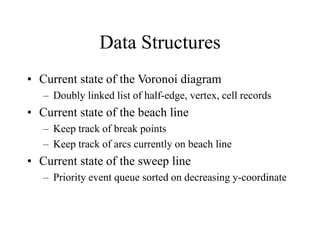
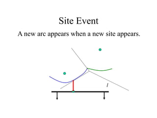
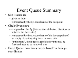
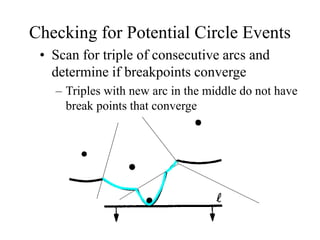
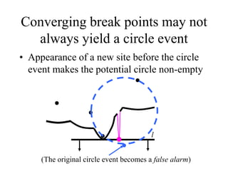
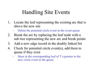
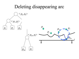
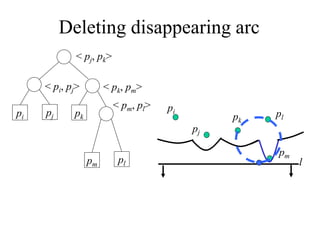
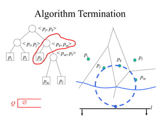
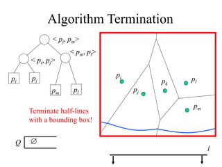
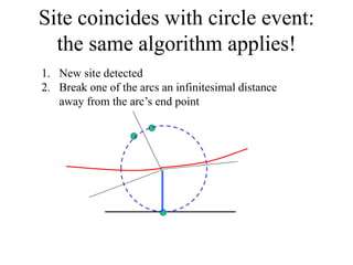
This document provides an overview of Voronoi diagrams, including: - Defining Voronoi diagrams as subdividing a plane into regions based on distance to input sites - Demonstrating Voronoi diagrams for 1, 2, and more sites - Explaining properties like cells, edges, and vertices - Analyzing the complexity and proving Voronoi diagrams have linear size - Outlining Fortune's sweep line algorithm for constructing Voronoi diagrams in linear time using data structures like a balanced binary search tree and doubly linked list

1. Lecture 7: Voronoi Diagrams
Presented by Allen Miu
6.838 Computational Geometry
September 27, 2001

2. Post Office: What is the area of service?
q
q : free point
e
e : Voronoi edge
v
v : Voronoi vertex
pi
pi : site points

3. Definition of Voronoi Diagram
• Let P be a set of n distinct points (sites) in the plane.
• The Voronoi diagram of P is the subdivision of the plane
into n cells, one for each site.
• A point q lies in the cell corresponding to a site pi  P
iff
Euclidean_Distance( q, pi ) < Euclidean_distance( q, pj ),
for each pi  P, j  i.

4. Demo
http://www.diku.dk/students/duff/Fortune/
http://www.msi.umn.edu/~schaudt/voronoi/
voronoi.html

5. Voronoi Diagram Example:
1 site

6. Two sites form a perpendicular
bisector
Voronoi Diagram is a line
that extends infinitely in
both directions, and the
two half planes on either
side.

7. Collinear sites form a series of
parallel lines

8. Non-collinear sites form Voronoi
half lines that meet at a vertex
A Voronoi vertex is
the center of an empty
circle touching 3 or
more sites.
v
Half lines
A vertex has
degree  3

9. Voronoi Cells and Segments
v

10. Voronoi Cells and Segments
v
Unbounded Cell
Bounded Cell
Segment

11. Who wants to be a Millionaire?
v
Which of the following is true for
2-D Voronoi diagrams?
Four or more non-collinear sites are…
1. sufficient to create a bounded cell
2. necessary to create a bounded cell
3. 1 and 2
4. none of above

12. Who wants to be a Millionaire?
v
Which of the following is true for
2-D Voronoi diagrams?
Four or more non-collinear sites are…
1. sufficient to create a bounded cell
2. necessary to create a bounded cell
3. 1 and 2
4. none of above

13. Degenerate Case:
no bounded cells!
v

14. Summary of Voronoi Properties
A point q lies on a Voronoi edge between sites pi and pj
iff the largest empty circle centered at q touches only
pi and pj
– A Voronoi edge is a subset of locus of points equidistant
from pi and pj
e
e : Voronoi edge
v
v : Voronoi vertex
pi
pi : site points

15. Summary of Voronoi Properties
A point q is a vertex iff the largest empty circle
centered at q touches at least 3 sites
– A Voronoi vertex is an intersection of 3 more segments,
each equidistant from a pair of sites
e
e : Voronoi edge
v
v : Voronoi vertex
pi
pi : site points

16. Outline
• Definitions and Examples
• Properties of Voronoi diagrams
• Complexity of Voronoi diagrams
• Constructing Voronoi diagrams
– Intuitions
– Data Structures
– Algorithm
• Running Time Analysis
• Demo
• Duality and degenerate cases

17. Voronoi diagrams have linear
complexity {|v|, |e| = O(n)}
Intuition: Not all bisectors are Voronoi edges!
e
e : Voronoi edge
pi
pi : site points

18. Voronoi diagrams have linear
complexity {|v|, |e| = O(n)}
Claim: For n  3, |v|  2n  5 and |e|  3n  6
Proof: (Easy Case)
…
Collinear sites  |v| = 0, |e| = n – 1

19. Voronoi diagrams have linear
complexity {|v|, |e| = O(n)}
Claim: For n  3, |v|  2n  5 and |e|  3n  6
Proof: (General Case)
• Euler’s Formula: for connected, planar graphs,
|v| – |e| + f = 2
Where:
|v| is the number of vertices
|e| is the number of edges
f is the number of faces

20. Voronoi diagrams have linear
complexity {|v|, |e| = O(n)}
Claim: For n  3, |v|  2n  5 and |e|  3n  6
Proof: (General Case)
• For Voronoi graphs, f = n  (|v| +1) – |e| + n = 2
e
pi
p
To apply Euler’s Formula, we
“planarize” the Voronoi diagram
by connecting half lines to
an extra vertex.

21. Voronoi diagrams have linear
complexity {|v|, |e| = O(n)}
Moreover,
and
so
together with
we get, for n  3
|
|
2
)
deg(
)
(
e
v
P
Vor
v




),
(P
Vor
v
 3
)
deg( 
v
)
1
|
(|
3
|
|
2 

 v
e
2
|
|
)
1
|
(| 


 n
e
v
6
3
|
|
5
2
|
|




n
e
n
v

22. Outline
• Definitions and Examples
• Properties of Voronoi diagrams
• Complexity of Voronoi diagrams
• Constructing Voronoi diagrams
– Intuitions
– Data Structures
– Algorithm
• Running Time Analysis
• Demo
• Duality and degenerate cases

23. Constructing Voronoi Diagrams
Given a half plane intersection algorithm…

24. Constructing Voronoi Diagrams
Given a half plane intersection algorithm…

25. Constructing Voronoi Diagrams
Given a half plane intersection algorithm…

26. Constructing Voronoi Diagrams
Given a half plane intersection algorithm…
Repeat for each site
Running Time:
O( n2 log n )

27. Constructing Voronoi Diagrams
• Half plane intersection O( n2 log n )
• Fortune’s Algorithm
– Sweep line algorithm
• Voronoi diagram constructed as horizontal line
sweeps the set of sites from top to bottom
• Incremental construction  maintains portion of
diagram which cannot change due to sites below
sweep line, keeping track of incremental changes for
each site (and Voronoi vertex) it “sweeps”

28. Constructing Voronoi Diagrams
What is the invariant we are looking for?
Maintain a representation of the locus of points q that
are closer to some site pi above the sweep line than to
the line itself (and thus to any site below the line).
e
v
pi
Sweep Line
q

29. Constructing Voronoi Diagrams
Which points are closer to a site above the sweep
line than to the sweep line itself?
Sweep Line
pi
q
The set of parabolic arcs form a beach-line that bounds
the locus of all such points
Equidistance

30. Constructing Voronoi Diagrams
Break points trace out Voronoi edges.
Equidistance
Sweep Line
pi
q

31. Constructing Voronoi Diagrams
Arcs flatten out as sweep line moves down.
Sweep Line
pi
q

32. Eventually, the middle arc disappears.
Constructing Voronoi Diagrams
Sweep Line
pi
q

33. We have detected a circle that is empty (contains no
sites) and touches 3 or more sites.
Constructing Voronoi Diagrams
Sweep Line
pi
q
Voronoi vertex!

34. Beach Line properties
• Voronoi edges are traced by the break points
as the sweep line moves down.
– Emergence of a new break point(s) (from
formation of a new arc or a fusion of two
existing break points) identifies a new edge
• Voronoi vertices are identified when two
break points meet (fuse).
– Decimation of an old arc identifies new vertex

35. Data Structures
• Current state of the Voronoi diagram
– Doubly linked list of half-edge, vertex, cell records
• Current state of the beach line
– Keep track of break points
– Keep track of arcs currently on beach line
• Current state of the sweep line
– Priority event queue sorted on decreasing y-coordinate

36. Doubly Linked List (D)
• Goal: a simple data structure that allows an
algorithm to traverse a Voronoi diagram’s
segments, cells and vertices
e
v
Cell(pi)

37. Doubly Linked List (D)
• Divide segments into uni-directional half-edges
• A chain of counter-clockwise half-edges forms a cell
• Define a half-edge’s “twin” to be its opposite half-edge of the
same segment
e
v
Cell(pi)

38. Doubly Linked List (D)
• Cell Table
– Cell(pi) : pointer to any incident half-edge
• Vertex Table
– vi : list of pointers to all incident half-edges
• Doubly Linked-List of half-edges; each has:
– Pointer to Cell Table entry
– Pointers to start/end vertices of half-edge
– Pointers to previous/next half-edges in the CCW chain
– Pointer to twin half-edge

39. Balanced Binary Tree (T)
• Internal nodes represent break points between two arcs
– Also contains a pointer to the D record of the edge being traced
• Leaf nodes represent arcs, each arc is in turn represented
by the site that generated it
– Also contains a pointer to a potential circle event
pi pj pk pl
< pj, pk>
< pi, pj> < pk, pl>
pi
pj
pk
pl
l

40. Event Queue (Q)
• An event is an interesting point encountered by the
sweep line as it sweeps from top to bottom
– Sweep line makes discrete stops, rather than a
continuous sweep
• Consists of Site Events (when the sweep line
encounters a new site point) and Circle Events
(when the sweep line encounters the bottom of an
empty circle touching 3 or more sites).
• Events are prioritized based on y-coordinate

41. Site Event
A new arc appears when a new site appears.
l

42. Site Event
A new arc appears when a new site appears.
l

43. Site Event
Original arc above the new site is broken into two
 Number of arcs on beach line is O(n)
l

44. Circle Event
An arc disappears whenever an empty circle touches
three or more sites and is tangent to the sweep line.
Sweep line helps determine that the circle is indeed empty.
Circle Event!
Sweep Line
pi
q
Voronoi vertex!

45. Event Queue Summary
• Site Events are
– given as input
– represented by the xy-coordinate of the site point
• Circle Events are
– computed on the fly (intersection of the two bisectors in
between the three sites)
– represented by the xy-coordinate of the lowest point of
an empty circle touching three or more sites
– “anticipated”, these newly generated events may be
false and need to be removed later
• Event Queue prioritizes events based on their y-
coordinates

46. Summarizing Data Structures
• Current state of the Voronoi diagram
– Doubly linked list of half-edge, vertex, cell records
• Current state of the beach line
– Keep track of break points
• Inner nodes of binary search tree; represented by a tuple
– Keep track of arcs currently on beach line
• Leaf nodes of binary search tree; represented by a site that
generated the arc
• Current state of the sweep line
– Priority event queue sorted on decreasing y-coordinate

47. Algorithm
1. Initialize
• Event queue Q  all site events
• Binary search tree T  
• Doubly linked list D  
2. While Q not ,
• Remove event (e) from Q with largest y-
coordinate
• HandleEvent(e, T, D)

48. Handling Site Events
1. Locate the existing arc (if any) that is above the
new site
2. Break the arc by replacing the leaf node with a
sub tree representing the new arc and its break
points
3. Add two half-edge records in the doubly linked
list
4. Check for potential circle event(s), add them to
event queue if they exist

49. Locate the existing arc that is above
the new site
pi pj pk pl
< pj, pk>
< pi, pj> < pk, pl>
• The x coordinate of the new site is used for the binary search
• The x coordinate of each breakpoint along the root to leaf path
is computed on the fly
pi
pj
pk
pl
l
pm

50. Break the Arc
pi pj pk
< pj, pk>
< pi, pj> < pk, pl>
Corresponding leaf replaced by a new sub-tree
pi
pj
pk
pl
l
pm
pm pl
< pl, pm>
< pm, pl>
pl
Different arcs can be identified
by the same site!

51. Add a new edge record in the doubly
linked list
pi pj pk
< pj, pk>
< pi, pj> < pk, pl>
pm pl
< pl, pm>
< pm, pl>
pl
pi
pj
pk
pl
l
pm
New Half Edge Record
Endpoints  
Pointers to two half-edge
records
l
pm

52. Checking for Potential Circle Events
• Scan for triple of consecutive arcs and
determine if breakpoints converge
– Triples with new arc in the middle do not have
break points that converge

53. Checking for Potential Circle Events
• Scan for triple of consecutive arcs and
determine if breakpoints converge
– Triples with new arc in the middle do not have
break points that converge

54. Checking for Potential Circle Events
• Scan for triple of consecutive arcs and
determine if breakpoints converge
– Triples with new arc in the middle do not have
break points that converge

55. Converging break points may not
always yield a circle event
• Appearance of a new site before the circle
event makes the potential circle non-empty
l
(The original circle event becomes a false alarm)

56. Handling Site Events
1. Locate the leaf representing the existing arc that is
above the new site
– Delete the potential circle event in the event queue
2. Break the arc by replacing the leaf node with a
sub tree representing the new arc and break points
3. Add a new edge record in the doubly linked list
4. Check for potential circle event(s), add them to
queue if they exist
– Store in the corresponding leaf of T a pointer to the
new circle event in the queue

57. Handling Circle Events
1. Add vertex to corresponding edge record in doubly
linked list
2. Delete from T the leaf node of the disappearing arc
and its associated circle events in the event queue
3. Create new edge record in doubly linked list
4. Check the new triplets formed by the former
neighboring arcs for potential circle events

58. A Circle Event
pi pj pk
< pj, pk>
< pi, pj> < pk, pl>
pi
pj
pk
pl
l
pm
pm pl
< pl, pm>
< pm, pl>
pl

59. Add vertex to corresponding edge record
pi pj pk
< pj, pk>
< pi, pj> < pk, pl>
pi
pj
pk
pl
l
pm
pm pl
< pl, pm>
< pm, pl>
pl
Half Edge Record
Endpoints.add(x, y)
Half Edge Record
Endpoints.add(x, y)
Link!

60. Deleting disappearing arc
pi pj pk
< pj, pk>
< pi, pj>
pi
pj
pk
pl
l
pm
pm pl
< pm, pl>

61. Deleting disappearing arc
pi pj pk
< pj, pk>
< pi, pj>
pi
pj
pk
pl
l
pm
pm pl
< pm, pl>
< pk, pm>

62. Create new edge record
pi pj pk
< pj, pk>
< pi, pj>
pi
pj
pk
pl
l
pm
pm pl
< pm, pl>
< pk, pm>
New Half Edge Record
Endpoints.add(x, y)
A new edge is traced out by the new
break point < pk, pm>

63. Check the new triplets for
potential circle events
pi pj pk
< pj, pk>
< pi, pj>
pi
pj
pk
pl
l
pm
pm pl
< pm, pl>
< pk, pm>
Q y
…
new circle event

64. Minor Detail
• Algorithm terminates when Q = , but the
beach line and its break points continue to
trace the Voronoi edges
– Terminate these “half-infinite” edges via a
bounding box

65. Algorithm Termination
pi pj pk
< pj, pk>
< pi, pj>
pi
pj
pk
pl
l
pm
pm pl
< pm, pl>
< pk, pm>
Q 

66. Algorithm Termination
pi pj
< pj, pm>
< pi, pj>
pi
pj
pk
pl
l
pm
pm pl
< pm, pl>
Q 

67. Algorithm Termination
pi pj
< pj, pm>
< pi, pj>
pi
pj
pk
pl
l
pm
pm pl
< pm, pl>
Q 
Terminate half-lines
with a bounding box!

68. Outline
• Definitions and Examples
• Properties of Voronoi diagrams
• Complexity of Voronoi diagrams
• Constructing Voronoi diagrams
– Intuitions
– Data Structures
– Algorithm
• Running Time Analysis
• Demo
• Duality and degenerate cases

69. Handling Site Events
1. Locate the leaf representing the existing arc
that is above the new site
– Delete the potential circle event in the event queue
2. Break the arc by replacing the leaf node with a
sub tree representing the new arc and break
points
3. Add a new edge record in the link list
4. Check for potential circle event(s), add them to
queue if they exist
– Store in the corresponding leaf of T a pointer to the
new circle event in the queue
Running Time
O(log n)
O(1)
O(1)
O(1)

70. Handling Circle Events
1. Delete from T the leaf node of the
disappearing arc and its associated
circle events in the event queue
2. Add vertex record in doubly link list
3. Create new edge record in doubly
link list
4. Check the new triplets formed by the
former neighboring arcs for potential
circle events
Running Time
O(log n)
O(1)
O(1)
O(1)

71. Total Running Time
• Each new site can generate at most two new
arcs
beach line can have at most 2n – 1 arcs
at most O(n) site and circle events in the queue
• Site/Circle Event Handler O(log n)
 O(n log n) total running time

72. Is Fortune’s Algorithm Optimal?
• We can sort numbers using any algorithm that
constructs a Voronoi diagram!
• Map input numbers to a position on the number
line. The resulting Voronoi diagram is doubly
linked list that forms a chain of unbounded cells in
the left-to-right (sorted) order.
-5 1 3 6 7
Number
Line

73. Outline
• Definitions and Examples
• Properties of Voronoi diagrams
• Complexity of Voronoi diagrams
• Constructing Voronoi diagrams
– Intuitions
– Data Structures
– Algorithm
• Running Time Analysis
• Demo
• Duality and degenerate cases

74. Voronoi Diagram/Convex Hull Duality
Sites sharing a half-infinite edge are convex hull vertices
e
v
pi

75. Degenerate Cases
• Events in Q share the same y-coordinate
– Can additionally sort them using x-coordinate
• Circle event involving more than 3 sites
– Current algorithm produces multiple degree 3
Voronoi vertices joined by zero-length edges
– Can be fixed in post processing

76. Degenerate Cases
• Site points are collinear (break points
neither converge or diverge)
– Bounding box takes care of this
• One of the sites coincides with the lowest
point of the circle event
– Do nothing

77. Site coincides with circle event:
the same algorithm applies!
1. New site detected
2. Break one of the arcs an infinitesimal distance
away from the arc’s end point

78. Site coincides with circle event

79. Summary
• Voronoi diagram is a useful planar
subdivision of a discrete point set
• Voronoi diagrams have linear complexity
and can be constructed in O(n log n) time
• Fortune’s algorithm (optimal)