Downloaded 14 times


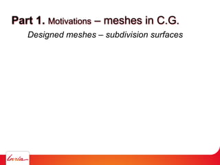


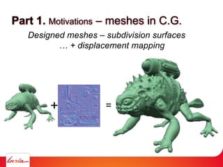


![Part 1. Motivations re-meshing
(Re)-meshing [Du et.al], [Alliez et.al], [Yan et.al ]](https://image.slidesharecdn.com/cgmeshing-191206193056/85/Meshing-for-computer-graphics-16-320.jpg)


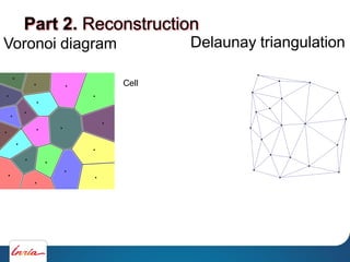
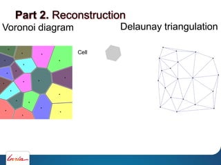


![Voronoi diagram
Amenta et.al, 1998]
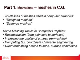
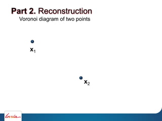
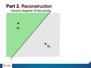
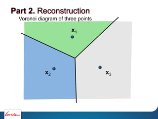
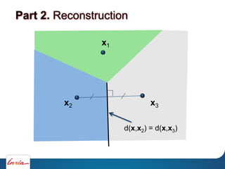
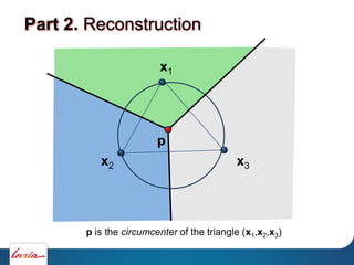
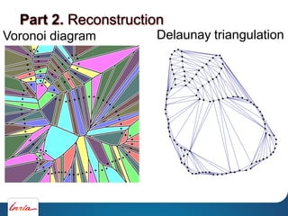
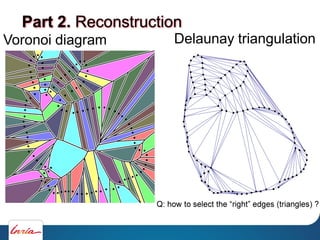
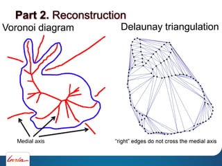
Part 2. Reconstruction
Delaunay triangulation](https://image.slidesharecdn.com/cgmeshing-191206193056/85/Meshing-for-computer-graphics-61-320.jpg)


![Amenta et.al 98]
1)Compute Del(X)
Part 2. Reconstruction](https://image.slidesharecdn.com/cgmeshing-191206193056/85/Meshing-for-computer-graphics-70-320.jpg)
![Amenta et.al 98]
1)Compute Del(X)
2)Compute the poles
Part 2. Reconstruction](https://image.slidesharecdn.com/cgmeshing-191206193056/85/Meshing-for-computer-graphics-71-320.jpg)
![Amenta et.al 98]
1)Compute Del(X)
2)Compute the poles
3)Compute Del(X U {poles})
Part 2. Reconstruction](https://image.slidesharecdn.com/cgmeshing-191206193056/85/Meshing-for-computer-graphics-72-320.jpg)
![Amenta et.al 98]
1)Compute Del(X)
2)Compute the poles
3)Compute Del(X U {poles})
4)Extract the triangles
Part 2. Reconstruction](https://image.slidesharecdn.com/cgmeshing-191206193056/85/Meshing-for-computer-graphics-73-320.jpg)
![Amenta et.al 98]
1)Compute Del(X)
2)Compute the poles
3)Compute Del(X U {poles})
4)Extract the triangles
- Amenta, Bern, Dey]
Part 2. Reconstruction](https://image.slidesharecdn.com/cgmeshing-191206193056/85/Meshing-for-computer-graphics-74-320.jpg)


![1. Reconstruction
Amenta, Bern, Kamvysselis 98]
Part 2. Reconstruction](https://image.slidesharecdn.com/cgmeshing-191206193056/85/Meshing-for-computer-graphics-78-320.jpg)
![1. Reconstruction
Amenta, Bern, Kamvysselis 98]
Further reading:
-
(See Nina Amenta, Tamal website)
eigencrust Kolluri and Shewchuk]
Boissonnat and Yvinec, Computational Geometry
Polygon Mesh Processing
Part 2. Reconstruction](https://image.slidesharecdn.com/cgmeshing-191206193056/85/Meshing-for-computer-graphics-79-320.jpg)
![1. ReconstructionPart 2. Reconstruction
This image: Poisson Surface Reconstruction [Kahzdan et.al, SGP 2006]
Implementation in CGAL (www.cgal.org)](https://image.slidesharecdn.com/cgmeshing-191206193056/85/Meshing-for-computer-graphics-80-320.jpg)


![Part 3. Re-meshing Centroidal Voronoi Tesselation
Color quantization
[Leung et.al, GPU Pro, AK Peters, 2010]](https://image.slidesharecdn.com/cgmeshing-191206193056/85/Meshing-for-computer-graphics-83-320.jpg)


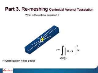


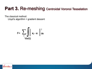
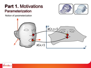
![The classical method:
F|xi = 2 mi (xi - gi) [Iri et.al], [Du et.al]
F=
Vor(i)
2
dxxi - x
i
Part 3. Re-meshing Centroidal Voronoi Tesselation](https://image.slidesharecdn.com/cgmeshing-191206193056/85/Meshing-for-computer-graphics-95-320.jpg)
![The classical method:
F|xi = 2 mi (xi - gi) [Iri et.al], [Du et.al]
Volume of Vor(i)
F=
Vor(i)
2
dxxi - x
i
Part 3. Re-meshing Centroidal Voronoi Tesselation](https://image.slidesharecdn.com/cgmeshing-191206193056/85/Meshing-for-computer-graphics-96-320.jpg)
![The classical method:
F|xi = 2 mi (xi - gi) [Iri et.al], [Du et.al]
Volume of Vor(i) Centroid of Vor(i)
F=
Vor(i)
2
dxxi - x
i
Part 3. Re-meshing Centroidal Voronoi Tesselation](https://image.slidesharecdn.com/cgmeshing-191206193056/85/Meshing-for-computer-graphics-97-320.jpg)
![The classical method:
F=
Vor(i)
2
dxxi - x
i
F|xi = 2 mi (xi - gi) [Iri et.al],
[Du et.al]
Volume of Vor(i) Centroid of Vor(i)
If xi coincides with the centroid of Vor(i),
we got a stationary point of F (therefore a « good sampling »)
Part 3. Re-meshing Centroidal Voronoi Tesselation](https://image.slidesharecdn.com/cgmeshing-191206193056/85/Meshing-for-computer-graphics-98-320.jpg)
![The classical method:
F=
Vor(i)
2
dxxi - x
i
F|xi = 2 mi (xi - gi) [Iri et.al],
[Du et.al]
Volume of Vor(i) Centroid of Vor(i)
If xi coincides with the centroid of Vor(i),
we got a stationary point of F (therefore a « good sampling »)
Vor(X): Centroidal Voronoi Tesselation
Part 3. Re-meshing Centroidal Voronoi Tesselation](https://image.slidesharecdn.com/cgmeshing-191206193056/85/Meshing-for-computer-graphics-99-320.jpg)


![(Geometric point of view)
Loop
Move the xi's to the gi's
Re-triangulate
End loop
+ Provably decreases F [Du et.al]
+ Reasonably easy to implement
- Slow (linear) convergence
Part 3. Re-meshing Centroidal Voronoi Tesselation](https://image.slidesharecdn.com/cgmeshing-191206193056/85/Meshing-for-computer-graphics-102-320.jpg)
![Part 3.
Idea:
Use method for minimizing the non-linear function F
[Liu, Wang, L, Yan, Lu, ACM TOG 2008]](https://image.slidesharecdn.com/cgmeshing-191206193056/85/Meshing-for-computer-graphics-103-320.jpg)
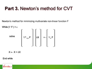


![Part 3.
Theorem: F is C2 almost everywhere
[Liu, Wang, L, Sun, Yan, Lu and Yang 09]](https://image.slidesharecdn.com/cgmeshing-191206193056/85/Meshing-for-computer-graphics-107-320.jpg)
![Part 3.
Theorem: F is C2 almost everywhere
[Liu, Wang, L, Sun, Yan, Lu and Yang 09]
If you want to know: it is not C2 when:
A bisector is aligned with an edge of the boundary
Two sites coincide [Du, Emelinanenko et.al, 2011]](https://image.slidesharecdn.com/cgmeshing-191206193056/85/Meshing-for-computer-graphics-108-320.jpg)


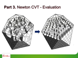


![Part 3.
CVT in 2D
CVT on surfaces
CVT in volumes
[Yan, Wang, L, Liu SIGGRAPH 2010]](https://image.slidesharecdn.com/cgmeshing-191206193056/85/Meshing-for-computer-graphics-118-320.jpg)

![2. Remeshing
Validity of Restricted Voronoi Diagram / Restricted Delaunay Triangulation
Theorem : [Edelsbrunner & Shah 1997]
Topological Ball Property: if each face of the
Restricted Voronoi Diagram is homeomorphic to a
disc, then the Restricted Delaunay Triangulation is
homeomorphic to the surface S
Part 3.](https://image.slidesharecdn.com/cgmeshing-191206193056/85/Meshing-for-computer-graphics-120-320.jpg)

![2. Remeshing
Validity of Restricted Voronoi Diagram / Restricted Delaunay Triangulation
Theorem : [Edelsbrunner & Shah 1997]
Topological Ball Property: if each k-face of the
Restricted Voronoi Diagram is homeomorphic to a
disc, then the Restricted Delaunay Triangulation is
homeomorphic to the surface S
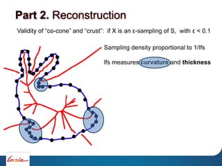
Theorem: [Amenta & Bern 1999]
if X is an -sampling of S, with < 0.1, then the Restricted
Delaunay triangulation is homeomorphic to the surface S
Part 3.](https://image.slidesharecdn.com/cgmeshing-191206193056/85/Meshing-for-computer-graphics-122-320.jpg)


![Part 3. Conclusions on Newton CVT
Sticking to the definition
(rather than the property)
Benefits:
Faster convergence
[Liu, Wang, L, Sun, Yan, Lu and Yang 09]
More general algorithm Chap. 4.](https://image.slidesharecdn.com/cgmeshing-191206193056/85/Meshing-for-computer-graphics-126-320.jpg)


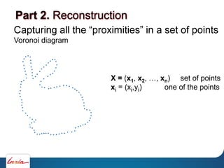
![Tet Meshing
1. Fully Automated
2. Millions of elements in
minutes/seconds
3. Adequate for some analysis
4. Inaccurate for other Analysis
Hex Meshing
1. Partially Automated, some Manual
2. Millions of elements in
days/weeks/months
3. Preferred by some analysts for solution
quality
[Matt Staten] (Sandial Labs)
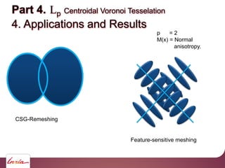
Part 4. Lp Centroidal Voronoi Tesselation
1. Motivations Why Hexes ?](https://image.slidesharecdn.com/cgmeshing-191206193056/85/Meshing-for-computer-graphics-129-320.jpg)


![F=
Vor(i)
2
dx(xi x)
i
Standard CVT:
F=
Vor(i)
p
dxM(x) (xi x)
i p
Lp CVT:
[L and Liu 2010]
Part 4. Lp Centroidal Voronoi Tesselation
3. Algorithm](https://image.slidesharecdn.com/cgmeshing-191206193056/85/Meshing-for-computer-graphics-133-320.jpg)


![1. Map the border to a convex polygon
2. Solve A u = u'
3. Solve A v = v'
Q: How do you choose
the coeffs. of A = [ai,j]
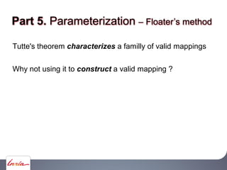
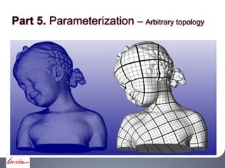
Part 5. Parameterization](https://image.slidesharecdn.com/cgmeshing-191206193056/85/Meshing-for-computer-graphics-151-320.jpg)

![[Greiner et.al]: Variational principles
for geometric modeling with Splines
PDEs for geometric optimization
Can we port this principle to
the discrete setting ? [Hormann & Greiner]
Part 5. Parameterization](https://image.slidesharecdn.com/cgmeshing-191206193056/85/Meshing-for-computer-graphics-153-320.jpg)


![JP =
x/ u
y/ u
z/ u
x/ v
y/ v
z/ v
[ ]
x/ u
x/ v
P
dxP(w)
u
v
w
dxP(w) = wu x/ u + wv x/ v = JP.w
u0,v0
Part 5. Parameterization Jacobian matrix JP](https://image.slidesharecdn.com/cgmeshing-191206193056/85/Meshing-for-computer-graphics-160-320.jpg)


![a
b
Jp =
x
u
x
v
y
u
y
v
z
u
z
v
= U V
t
a 0
0 b
0 0
Singular values decomposition (SVD) of J
Rem: Ip = Jt.J a = 1 ; b = 2
See also
[Hormann]
Part 5. Parameterization Eigen structure of GP](https://image.slidesharecdn.com/cgmeshing-191206193056/85/Meshing-for-computer-graphics-168-320.jpg)


![[Hormann & Greiner]
[Maillot & Verroust]
[Sander & Hoppe]
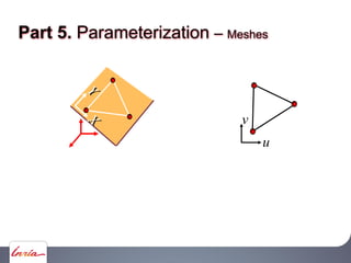
Part 5. Parameterization Meshes](https://image.slidesharecdn.com/cgmeshing-191206193056/85/Meshing-for-computer-graphics-174-320.jpg)
![[Hormann & Greiner]
[Maillot & Verroust]
[Sander & Hoppe]
Part 5. Parameterization Meshes](https://image.slidesharecdn.com/cgmeshing-191206193056/85/Meshing-for-computer-graphics-175-320.jpg)
![aij = 1
mean value coordinates[Floater]
The only one with th. guarantees
Part 5. Parameterization Meshes](https://image.slidesharecdn.com/cgmeshing-191206193056/85/Meshing-for-computer-graphics-176-320.jpg)


![Minimize
2
u
x
v
y
u
y-
v
x
-
T
Part 5. Parameterization Least Squares Conformal Maps
[L, Petitjean, Ray Maillot 2002]](https://image.slidesharecdn.com/cgmeshing-191206193056/85/Meshing-for-computer-graphics-181-320.jpg)
![Minimize
2
u
x
v
y
u
y-
v
x
-
T
Part 5. Parameterization Least Squares Conformal Maps
[L, Petitjean, Ray Maillot 2002]](https://image.slidesharecdn.com/cgmeshing-191206193056/85/Meshing-for-computer-graphics-182-320.jpg)

![Variables: angles
characterization of planar triangulation
Part 5. Parameterization Geometric Methods
Angle Based Flattening [Sheffer & De Sturler]](https://image.slidesharecdn.com/cgmeshing-191206193056/85/Meshing-for-computer-graphics-184-320.jpg)
![Cut by Seamster
[Sheffer & Hart]
initial ABF [Sheffer & de Sturler]
faster one [Sheffer et.al 04]
linABF [Zayer et.al 07]
u
v
Part 5. Parameterization Geometric Methods](https://image.slidesharecdn.com/cgmeshing-191206193056/85/Meshing-for-computer-graphics-185-320.jpg)


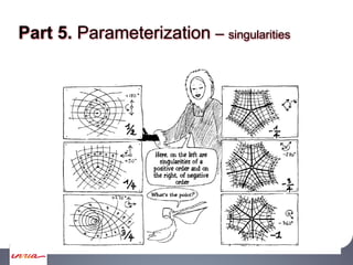

![Poincarré Hopf
N-Symmetry
direction fields
[Ray et.al]
See also N-Rosy
[Zhang et.al]
Part 5. Parameterization singularities](https://image.slidesharecdn.com/cgmeshing-191206193056/85/Meshing-for-computer-graphics-195-320.jpg)

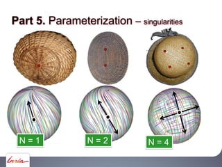


![Extension of the Poincaré-Hopf
theorem to N-symmetry
Discrete Index theory
[Ray et.al, ACM TOG 2008]
I = 2-2g
Design with full topology control
3/4
1/4
-1/4
Controlled influence of geometry/topology [Ray et.al, ACM TOG 2009]
Index Genus
Part 5. Parameterization singularities](https://image.slidesharecdn.com/cgmeshing-191206193056/85/Meshing-for-computer-graphics-203-320.jpg)
![Extension of the Poincaré-Hopf
theorem to N-symmetry
Discrete Index theory
[Ray et.al, ACM TOG 2008]
I = 2-2g
Design with full topology control
3/4
1/4
-1/4
Controlled influence of geometry/topology [Ray et.al, ACM TOG 2009]
Index Genus
Part 5. Parameterization singularities
See also this IMR, Kovalski, Ledoux and Frey, PDE-based quad meshing](https://image.slidesharecdn.com/cgmeshing-191206193056/85/Meshing-for-computer-graphics-204-320.jpg)


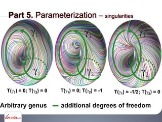
![Guidance vector fields
Part 5. Parameterization singularities
Periodic Global Parameterization [Ray et.al, 2006]](https://image.slidesharecdn.com/cgmeshing-191206193056/85/Meshing-for-computer-graphics-207-320.jpg)
![( ) : Parametric coordinates
Part 5. Parameterization singularities
Periodic Global Parameterization [Ray et.al, 2006]](https://image.slidesharecdn.com/cgmeshing-191206193056/85/Meshing-for-computer-graphics-208-320.jpg)
![Part 5. Parameterization singularities
Periodic Global Parameterization [Ray et.al, 2006]](https://image.slidesharecdn.com/cgmeshing-191206193056/85/Meshing-for-computer-graphics-209-320.jpg)
![Part 5. Parameterization singularities
Periodic Global Parameterization [Ray et.al, 2006]](https://image.slidesharecdn.com/cgmeshing-191206193056/85/Meshing-for-computer-graphics-210-320.jpg)
![Part 5. Parameterization singularities
Periodic Global Parameterization [Ray et.al, 2006]](https://image.slidesharecdn.com/cgmeshing-191206193056/85/Meshing-for-computer-graphics-211-320.jpg)
![Polycubemaps
Semi-manual construction[Tarini et.al]
Part 5. Parameterization quad base complex](https://image.slidesharecdn.com/cgmeshing-191206193056/85/Meshing-for-computer-graphics-212-320.jpg)


Three sentences: The document summarizes techniques for meshing and re-meshing used in computer graphics. It discusses using Voronoi diagrams and Delaunay triangulations to reconstruct meshes from point clouds, and using centroidal Voronoi tessellations to improve existing meshes through re-meshing by minimizing quantization noise. The document outlines methods for reconstruction, re-meshing scanned meshes, and converting meshes to subdivision surfaces.


![Human Reproduction [ Reproductive System ] Notes @irfanullah_mehar Irfanullah...](https://cdn.slidesharecdn.com/ss_thumbnails/humanreproductionreproductivesystemnotesirfanullahmeharirfanullahmeharjanantantra-260111172350-56e85778-thumbnail.jpg?width=640&height=640&fit=bounds)


