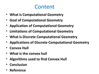
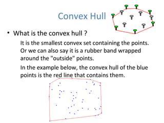
By
Saurav Mistry
Content
• What is Computational Geometry
• Goal of Computational Geometry
• Application of Computational Geometry
• Limitations of Computational Geometry
• What is Discrete Computational Geometry
• Applications of Discrete Computational Geometry
• Convex Hull
• What is the convex hull
• Algorithms used to find Convex Hull
• Conclusion
• Reference
What is Computational Geometry
• The study to describe algorithms for
manipulating curves and surfaces in solid
modeling
• In other words, it is used to describe the
subfield of algorithm theory that involves
the design and analysis of efficient
algorithms for problems involving
geometric input and digital output
Goal of Computational Geometry
 Computational geometry deals primarily with
straight or flat geometrical objects.
 It provide the basic geometric tools needed from
which application areas can then build their
programs
Application of Computational
Geometry
 It is used in solving problems of a geometric nature such
as in :-
computer graphics
computer vision
image processing.
 It is also used in
Robotics
Geographic information systems
Limitations of Computational
Geometry
 It deals with straight or flat objects only
 It primarily focus on 2-dimensional problems, and
3-dimensional problems to a limited extent
 It fails to deal with applications areas which require
discrete approximation to continuous phenomenon
What is Discrete Computational
Geometry
 It is the use of computational geometry with
contrast to ‘continuous’ phenomenon, for
example, smooth surfaces. Thus, it is termed as
Discrete Computational Geometry.
 It bridge the gap between computer
representation and geometric calculation.
Applications of Discrete
Computational Geometry
Discrete Computational Geometry mainly
deals with the following :-
• Convex hulls
• Triangulations
• Voronoi diagrams
• Polyhedra
• Polygons
Convex Hull
• What is the convex hull ?
It is the smallest convex set containing the points.
Or we can also say it is a rubber band wrapped
around the "outside" points.
In the example below, the convex hull of the blue
points is the red line that contains them.
Algorithms used to find Convex Hull
• Jarvis March
• Graham’s Scan
• Divide and Conquer
Jarvis March
ALGORITHM
• Start at some extreme point, which is guaranteed to be on
the hull.
• At each step, test each of the points, and find the one which
makes the largest right-hand turn. That point has to be the
next one on the hull.
Because this process marches around the hull in counter
clockwise order, like a ribbon wrapping itself around the
points, this algorithm also called the "gift-wrapping"
algorithm.Example:
http://www.cs.princeton.edu/courses/archive/spr10/cos226/demo
Efficiency of Jarvis March
• Proposed by R.A. Jarvis in 1973
• O(nh) complexity, with n being the total number of
points in the set, and h being the number of points
that lie in the convex hull.
• The worst case for this algorithm is denoted by O(n2
),
which is not optimal.
• Favorable conditions –
– very low number of total points
– low number of points on the convex hull
Graham’s Scan
ALGORITHM
• Find an extreme point. This point will be the pivot, is
guaranteed to be on the hull, and is chosen to be the point
with largest y coordinate.
• Sort the points in order of increasing angle about the pivot.
We end up with a star-shaped polygon (one in which one
special point, in this case the pivot, can "see" the whole
polygon).
• Build the hull, by marching around the star-shaped poly,
adding edges when we make a left turn, and back-tracking
when we make a right turn.
• http://www.cs.princeton.edu/courses/archive/fall08/cos226/demo
Efficiency of Graham’s Scan
• In the Graham’s Scan, the first phase of sorting
points by angle around the anchor point is of time
O(n logn) complexity.
• Phase 2 of this algorithm has a time complexity of
O(n).
• The total time complexity for this algorithm is O(n
logn) which is much more efficient than a worse case
scenario of Jarvis march at O(n2
).
Divide and Conquer
ALGORITHM
• Two separate hulls are created, one for the leftmost half of
the points, and one for the rightmost half.
• To divide in halves, sort by x-coordinates and find the median.
If there is an odd number of points, the leftmost half should
have the extra point.
• Recursively find the convex hull for the left set of points and
the right set of points. This gives hull A and hull B.
• Stitch together the two hulls to form the hull of the entire set.
• http://www.cse.unsw.edu.au/~lambert/java/3d/divideandconquer
Efficiency of Divide and Conquer
• The divide and conquer algorithm is also of time
complexity O( n logn).
• This algorithm is often used for cases in 3-D.
• A technicality of the divide and conquer method lies
in how many points are in the set. If the set has less
than four points, there is no need to sort the points,
but rather for these special cases, determine the hull
separately.
• A downside to this algorithm is the association of
recursive function calls.
Conclusion
• As it a new domain of study it is still under
research.
• However it has a great future in biology and
statistics.
Reference
• http://www.authorstream.com/Presentation/anupam999-1418956-discrete
• http://www.slideshare.net/9474778311/discrete-computational-geometry-3
• http://en.wikipedia.org/wiki/discrete_computational_geometry
• http://www.webopedia.com/TERM/Qdiscrete-computational-
geometry.html
• http://searchsecurity.techtarget.com/definition/discrete-
computational-geometry
Discrete Computaional Geometry

Discrete Computaional Geometry

  • 1.
  • 2.
    Content • What isComputational Geometry • Goal of Computational Geometry • Application of Computational Geometry • Limitations of Computational Geometry • What is Discrete Computational Geometry • Applications of Discrete Computational Geometry • Convex Hull • What is the convex hull • Algorithms used to find Convex Hull • Conclusion • Reference
  • 3.
    What is ComputationalGeometry • The study to describe algorithms for manipulating curves and surfaces in solid modeling • In other words, it is used to describe the subfield of algorithm theory that involves the design and analysis of efficient algorithms for problems involving geometric input and digital output
  • 4.
    Goal of ComputationalGeometry  Computational geometry deals primarily with straight or flat geometrical objects.  It provide the basic geometric tools needed from which application areas can then build their programs
  • 5.
    Application of Computational Geometry It is used in solving problems of a geometric nature such as in :- computer graphics computer vision image processing.  It is also used in Robotics Geographic information systems
  • 6.
    Limitations of Computational Geometry It deals with straight or flat objects only  It primarily focus on 2-dimensional problems, and 3-dimensional problems to a limited extent  It fails to deal with applications areas which require discrete approximation to continuous phenomenon
  • 7.
    What is DiscreteComputational Geometry  It is the use of computational geometry with contrast to ‘continuous’ phenomenon, for example, smooth surfaces. Thus, it is termed as Discrete Computational Geometry.  It bridge the gap between computer representation and geometric calculation.
  • 8.
    Applications of Discrete ComputationalGeometry Discrete Computational Geometry mainly deals with the following :- • Convex hulls • Triangulations • Voronoi diagrams • Polyhedra • Polygons
  • 9.
    Convex Hull • Whatis the convex hull ? It is the smallest convex set containing the points. Or we can also say it is a rubber band wrapped around the "outside" points. In the example below, the convex hull of the blue points is the red line that contains them.
  • 10.
    Algorithms used tofind Convex Hull • Jarvis March • Graham’s Scan • Divide and Conquer
  • 11.
    Jarvis March ALGORITHM • Startat some extreme point, which is guaranteed to be on the hull. • At each step, test each of the points, and find the one which makes the largest right-hand turn. That point has to be the next one on the hull. Because this process marches around the hull in counter clockwise order, like a ribbon wrapping itself around the points, this algorithm also called the "gift-wrapping" algorithm.Example: http://www.cs.princeton.edu/courses/archive/spr10/cos226/demo
  • 12.
    Efficiency of JarvisMarch • Proposed by R.A. Jarvis in 1973 • O(nh) complexity, with n being the total number of points in the set, and h being the number of points that lie in the convex hull. • The worst case for this algorithm is denoted by O(n2 ), which is not optimal. • Favorable conditions – – very low number of total points – low number of points on the convex hull
  • 13.
    Graham’s Scan ALGORITHM • Findan extreme point. This point will be the pivot, is guaranteed to be on the hull, and is chosen to be the point with largest y coordinate. • Sort the points in order of increasing angle about the pivot. We end up with a star-shaped polygon (one in which one special point, in this case the pivot, can "see" the whole polygon). • Build the hull, by marching around the star-shaped poly, adding edges when we make a left turn, and back-tracking when we make a right turn. • http://www.cs.princeton.edu/courses/archive/fall08/cos226/demo
  • 14.
    Efficiency of Graham’sScan • In the Graham’s Scan, the first phase of sorting points by angle around the anchor point is of time O(n logn) complexity. • Phase 2 of this algorithm has a time complexity of O(n). • The total time complexity for this algorithm is O(n logn) which is much more efficient than a worse case scenario of Jarvis march at O(n2 ).
  • 15.
    Divide and Conquer ALGORITHM •Two separate hulls are created, one for the leftmost half of the points, and one for the rightmost half. • To divide in halves, sort by x-coordinates and find the median. If there is an odd number of points, the leftmost half should have the extra point. • Recursively find the convex hull for the left set of points and the right set of points. This gives hull A and hull B. • Stitch together the two hulls to form the hull of the entire set. • http://www.cse.unsw.edu.au/~lambert/java/3d/divideandconquer
  • 16.
    Efficiency of Divideand Conquer • The divide and conquer algorithm is also of time complexity O( n logn). • This algorithm is often used for cases in 3-D. • A technicality of the divide and conquer method lies in how many points are in the set. If the set has less than four points, there is no need to sort the points, but rather for these special cases, determine the hull separately. • A downside to this algorithm is the association of recursive function calls.
  • 17.
    Conclusion • As ita new domain of study it is still under research. • However it has a great future in biology and statistics.
  • 18.
    Reference • http://www.authorstream.com/Presentation/anupam999-1418956-discrete • http://www.slideshare.net/9474778311/discrete-computational-geometry-3 •http://en.wikipedia.org/wiki/discrete_computational_geometry • http://www.webopedia.com/TERM/Qdiscrete-computational- geometry.html • http://searchsecurity.techtarget.com/definition/discrete- computational-geometry