Download as PDF, PPTX


![Meshing Counter-intuition
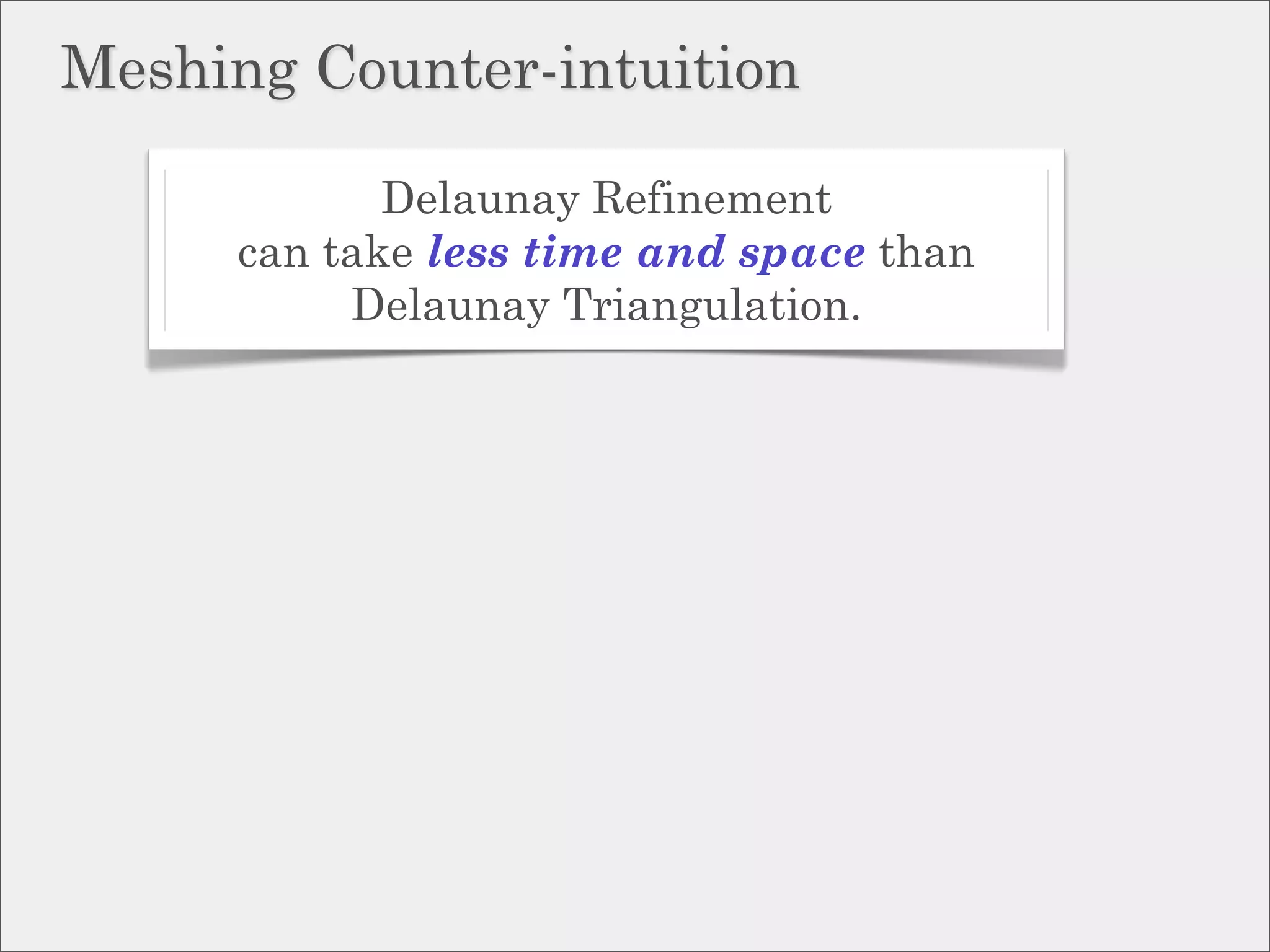
Delaunay Refinement
can take less time and space than
Delaunay Triangulation.
Theorem [Hudson, Miller, Phillips, ’06]:
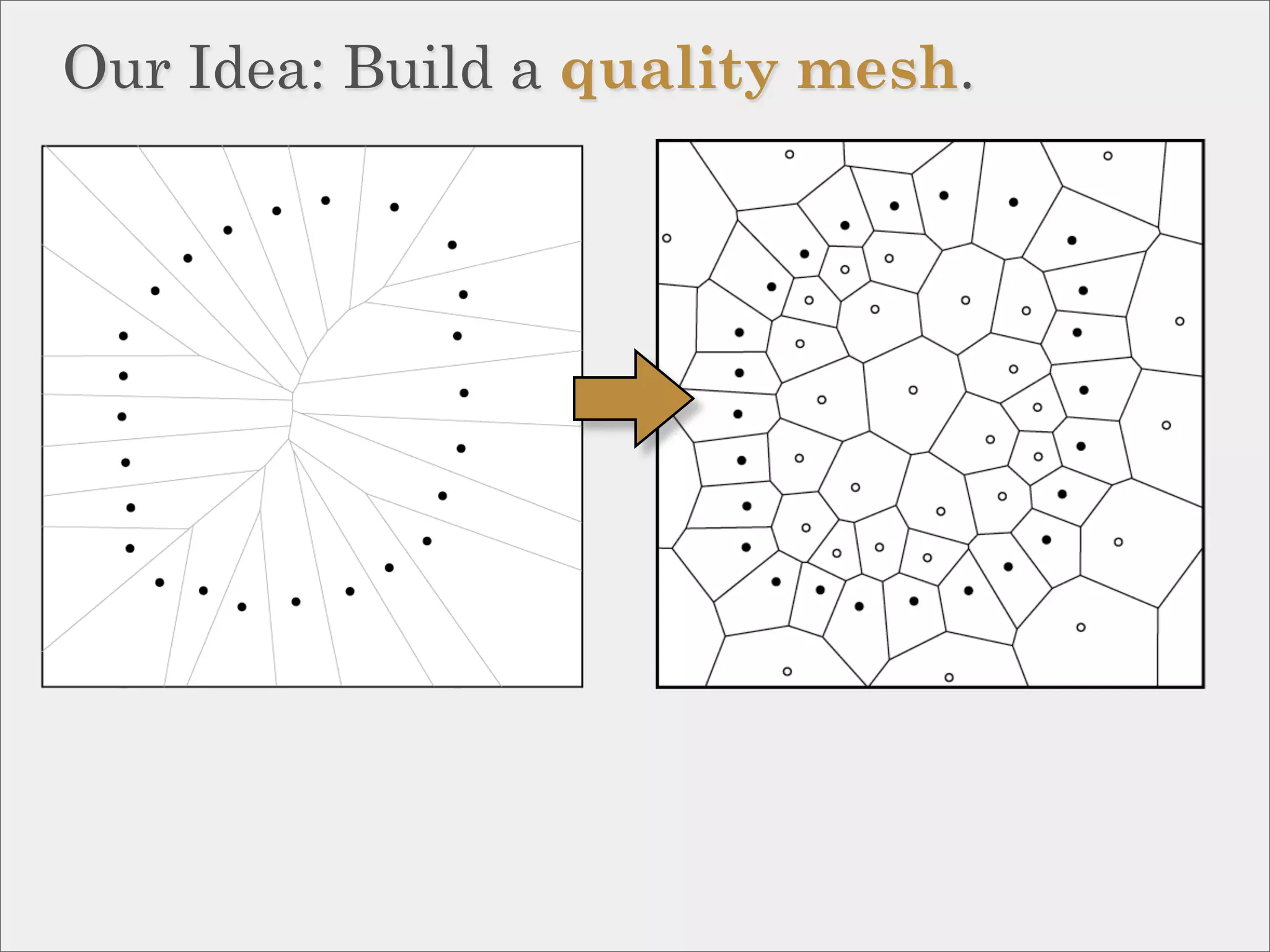
A quality mesh of a point set can
be constructed in O(n log ∆) time,
where ∆ is the spread.](https://image.slidesharecdn.com/socg10topological-100622141903-phpapp02/75/Topological-Inference-via-Meshing-39-2048.jpg)
![Meshing Counter-intuition
Delaunay Refinement
can take less time and space than
Delaunay Triangulation.
Theorem [Hudson, Miller, Phillips, ’06]:
A quality mesh of a point set can
be constructed in O(n log ∆) time,
where ∆ is the spread.
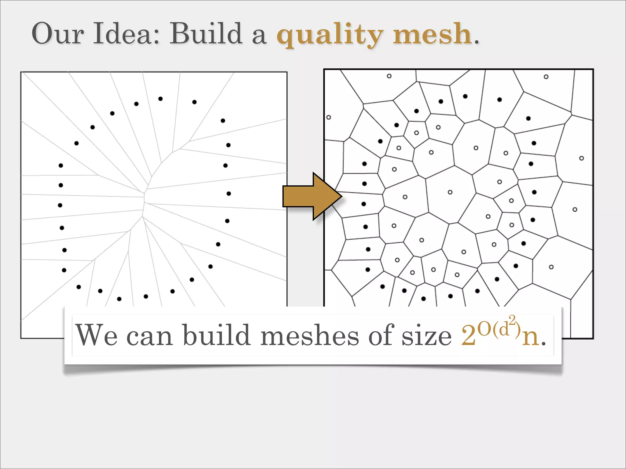
Theorem [Miller, Phillips, Sheehy, ’08]:
A quality mesh of a well-paced
point set has size O(n).](https://image.slidesharecdn.com/socg10topological-100622141903-phpapp02/75/Topological-Inference-via-Meshing-40-2048.jpg)

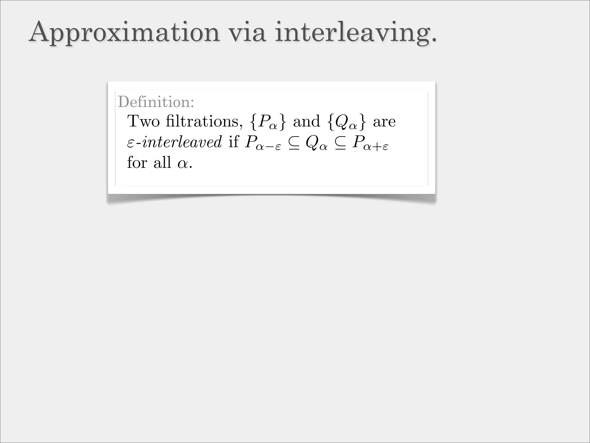
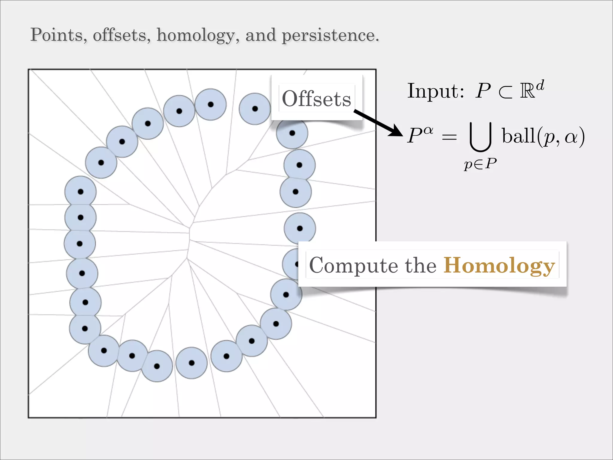
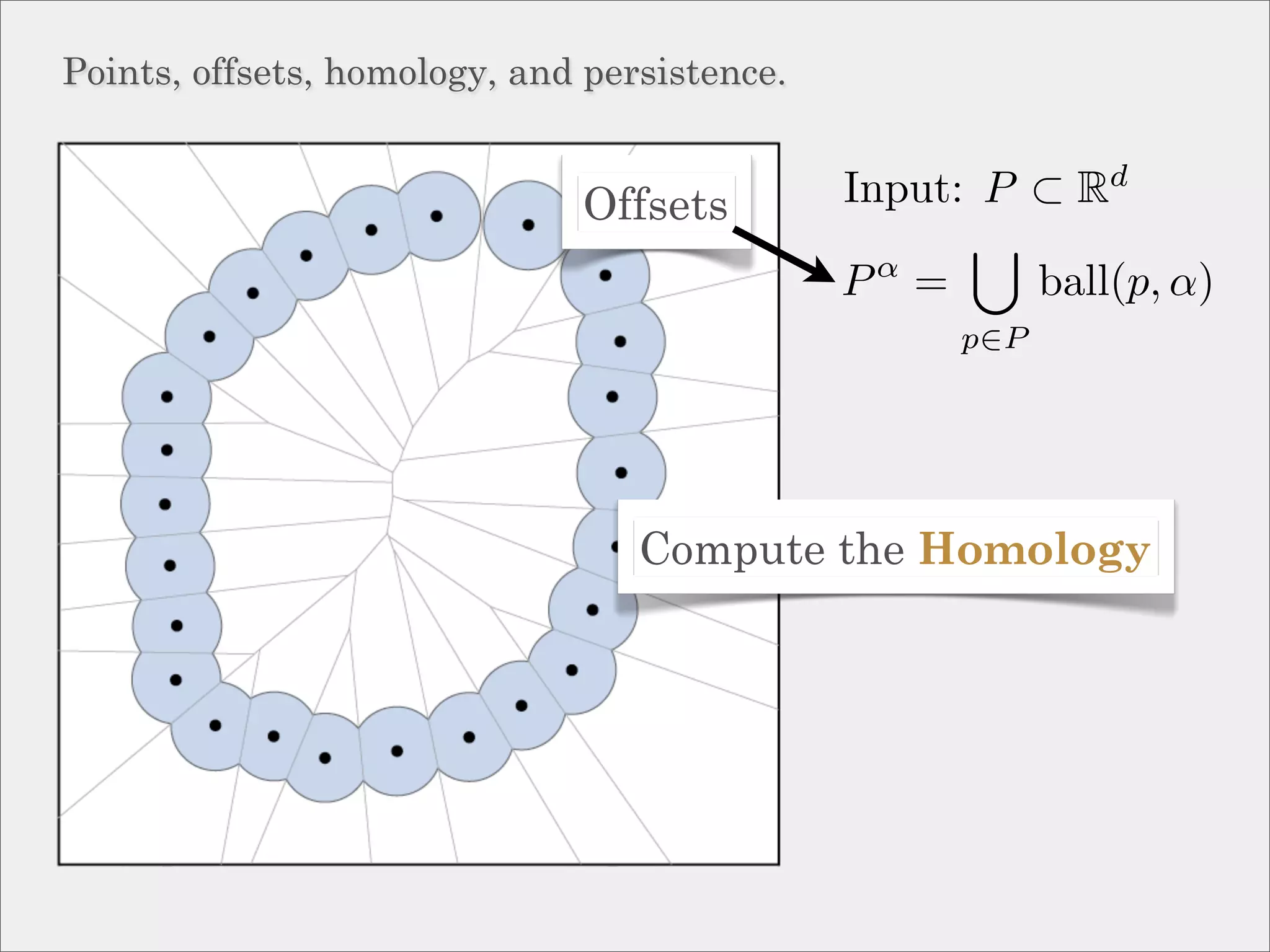
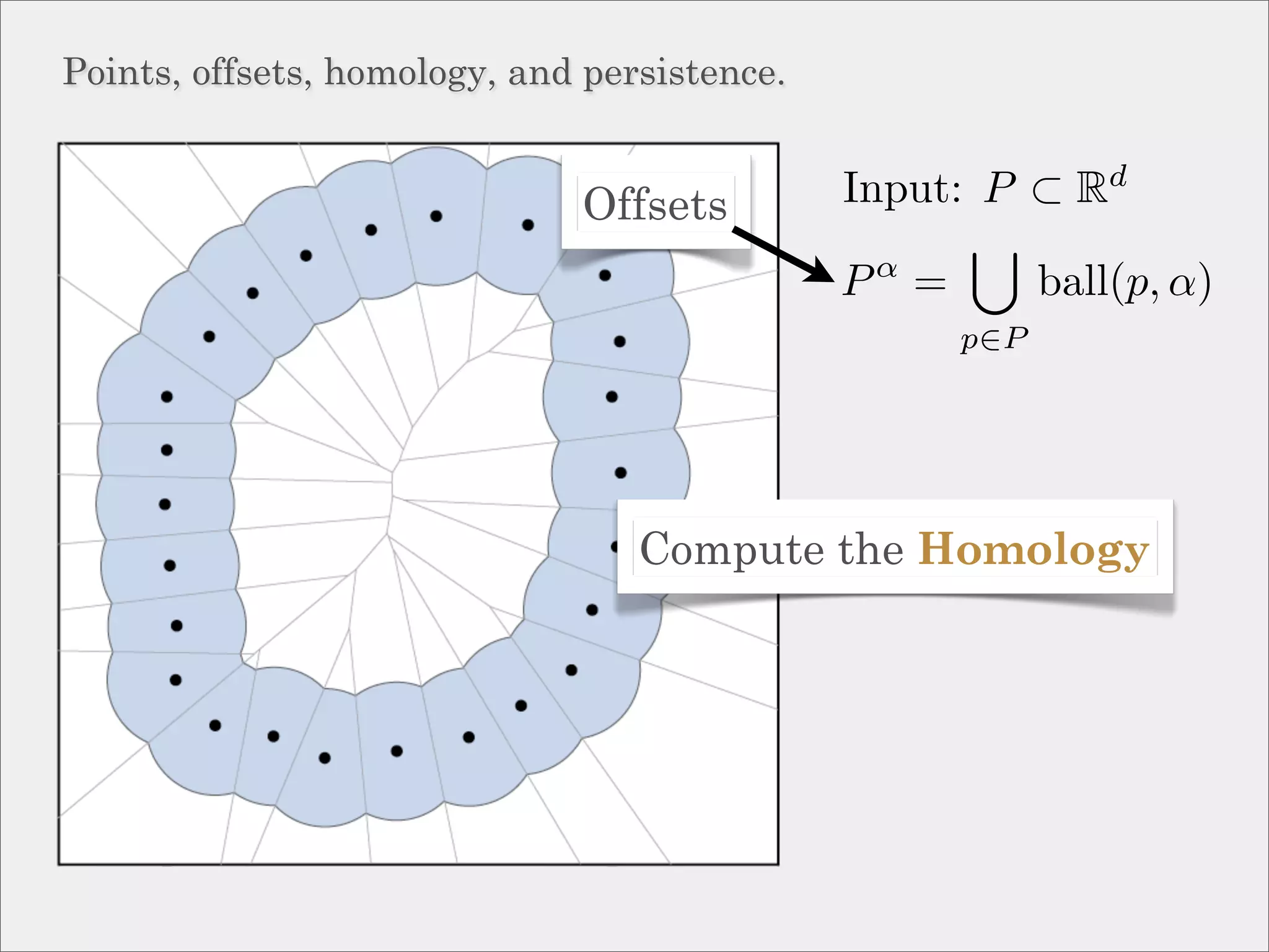
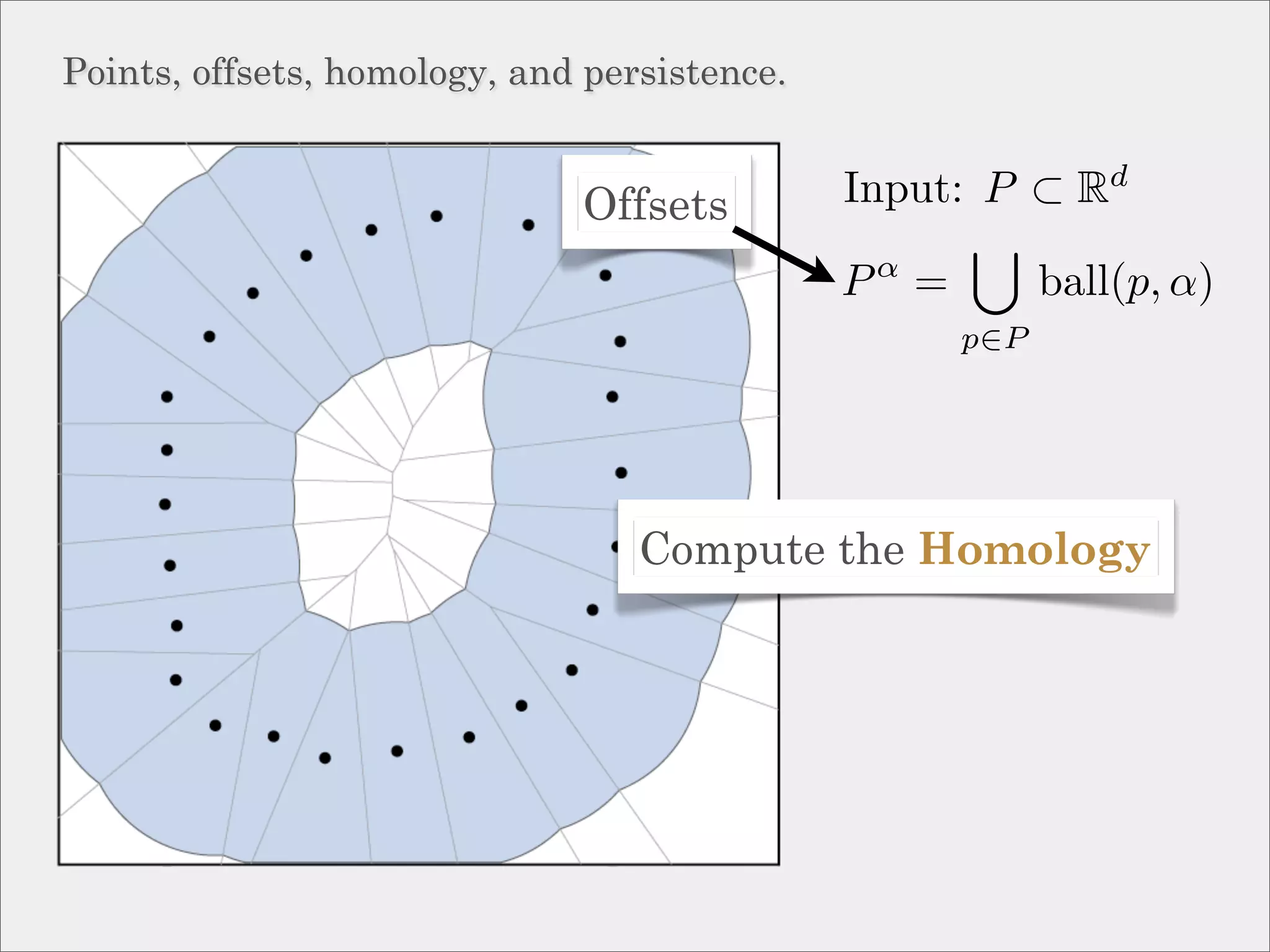
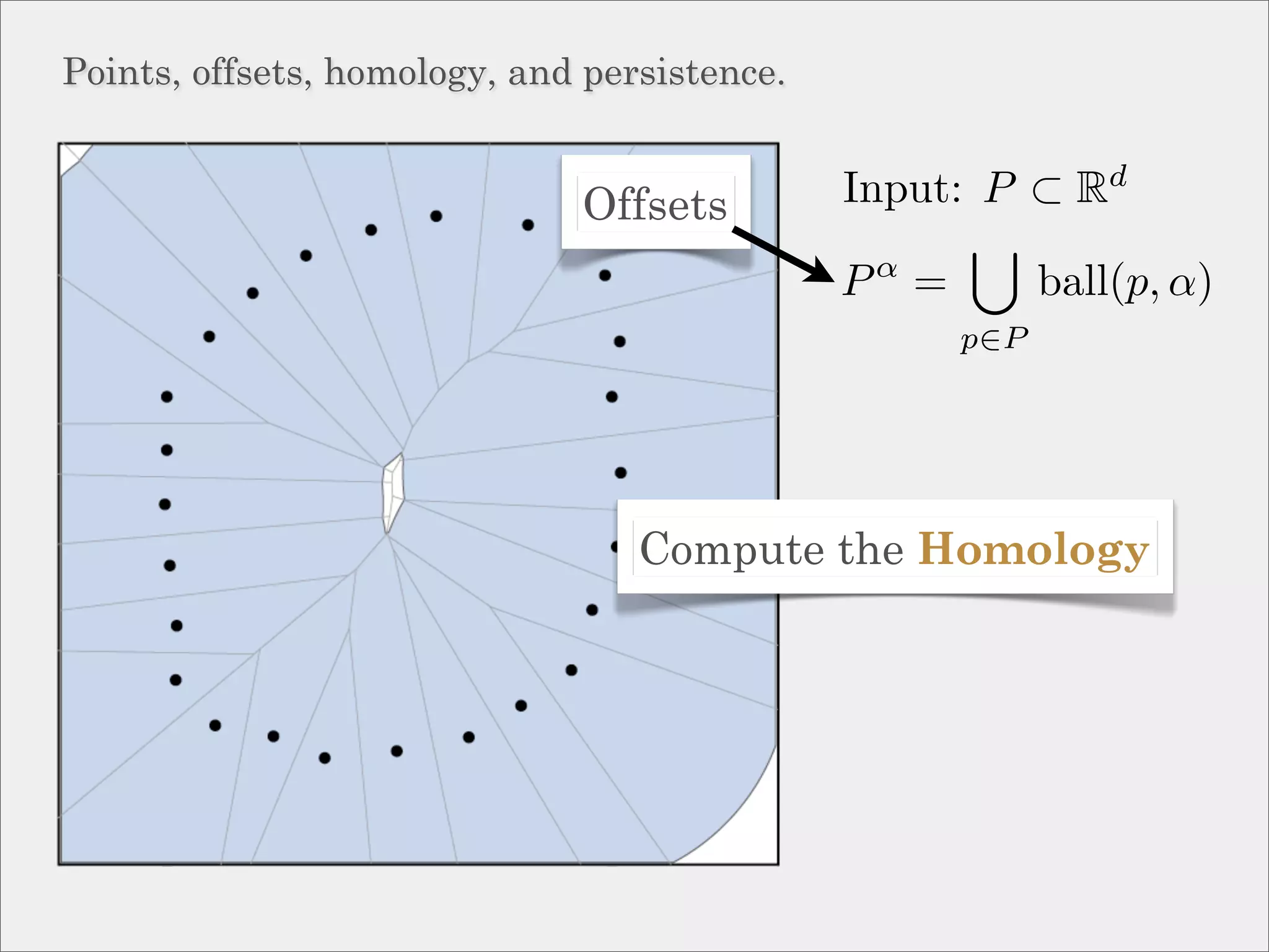
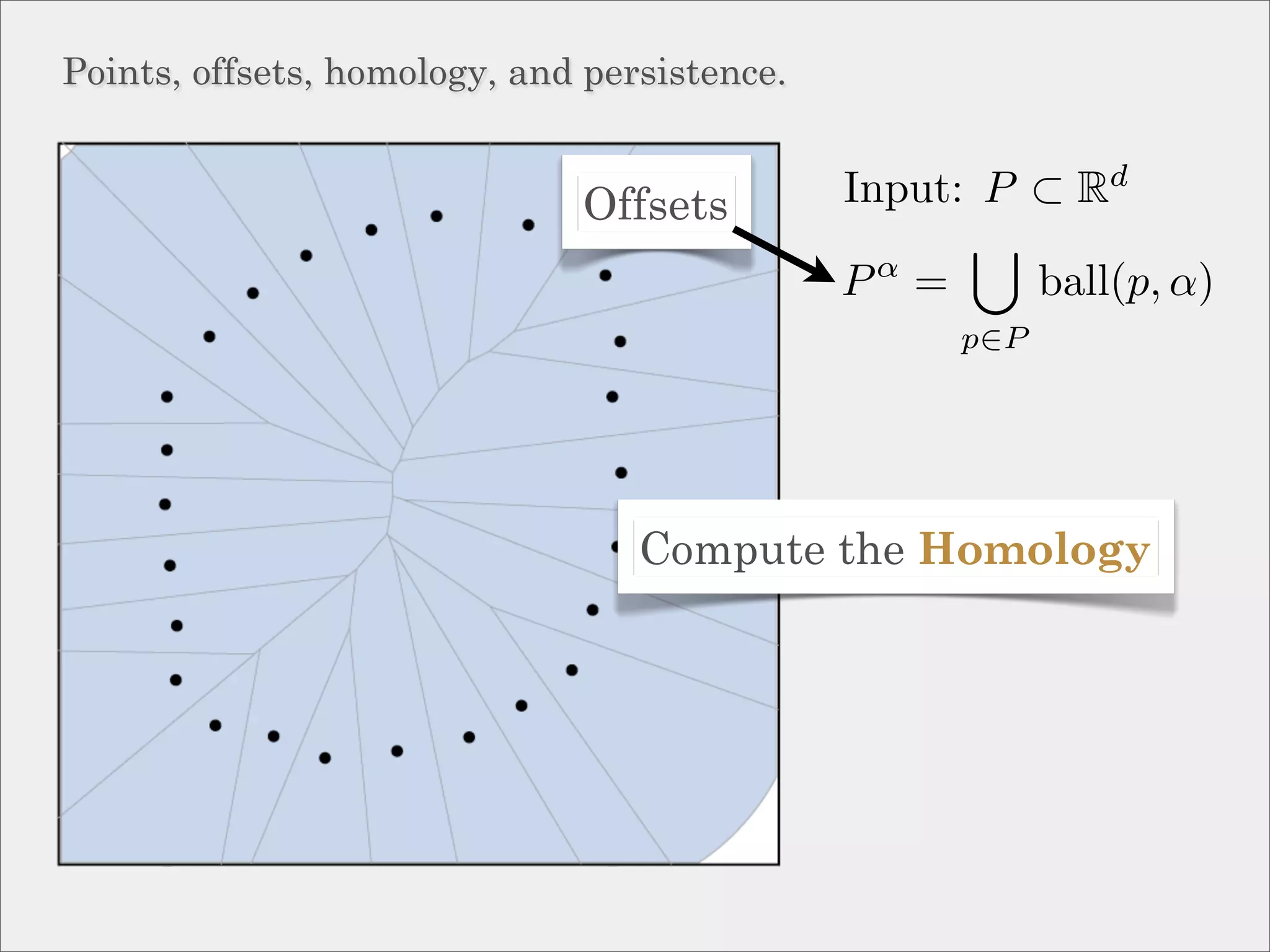
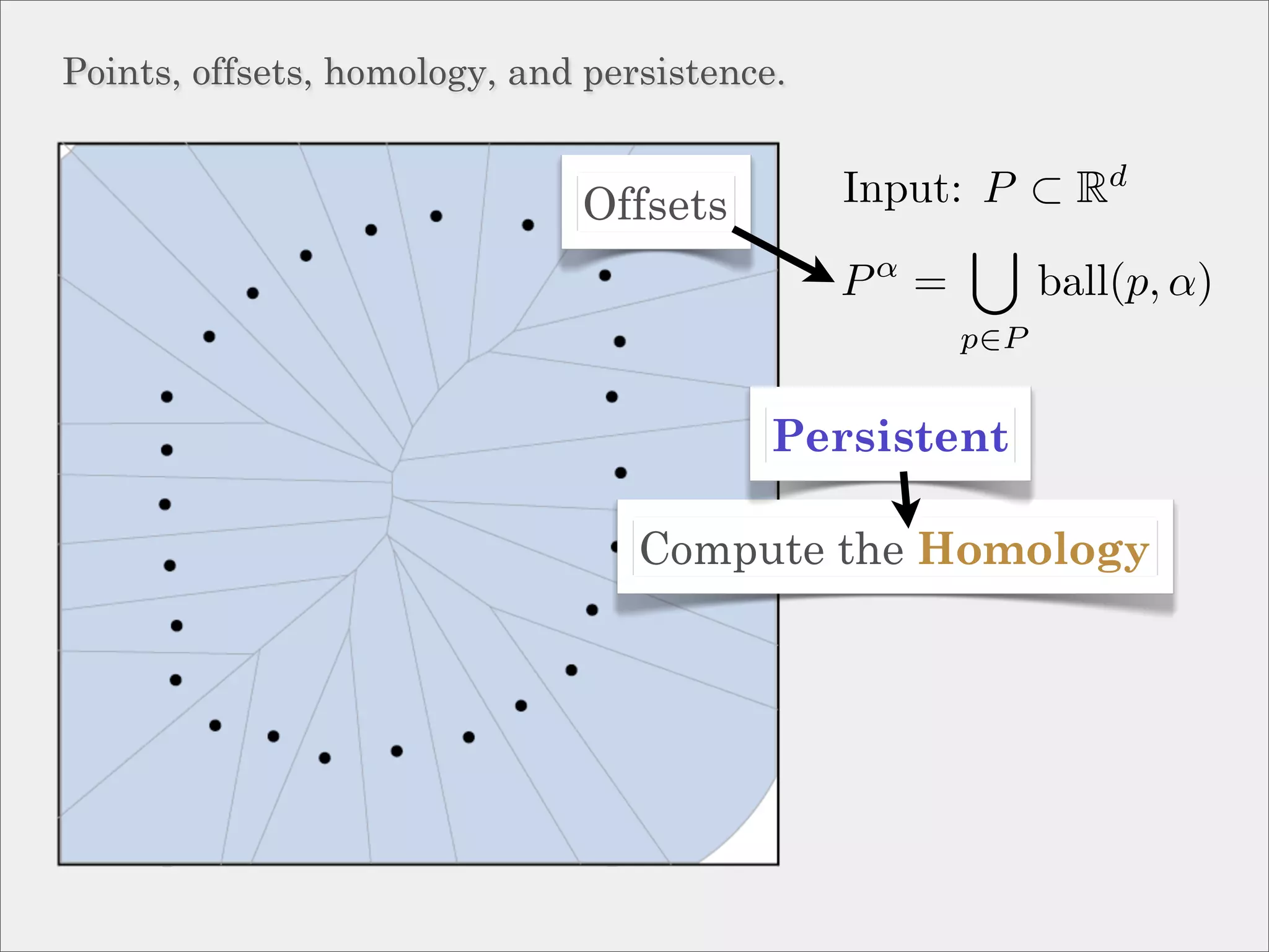
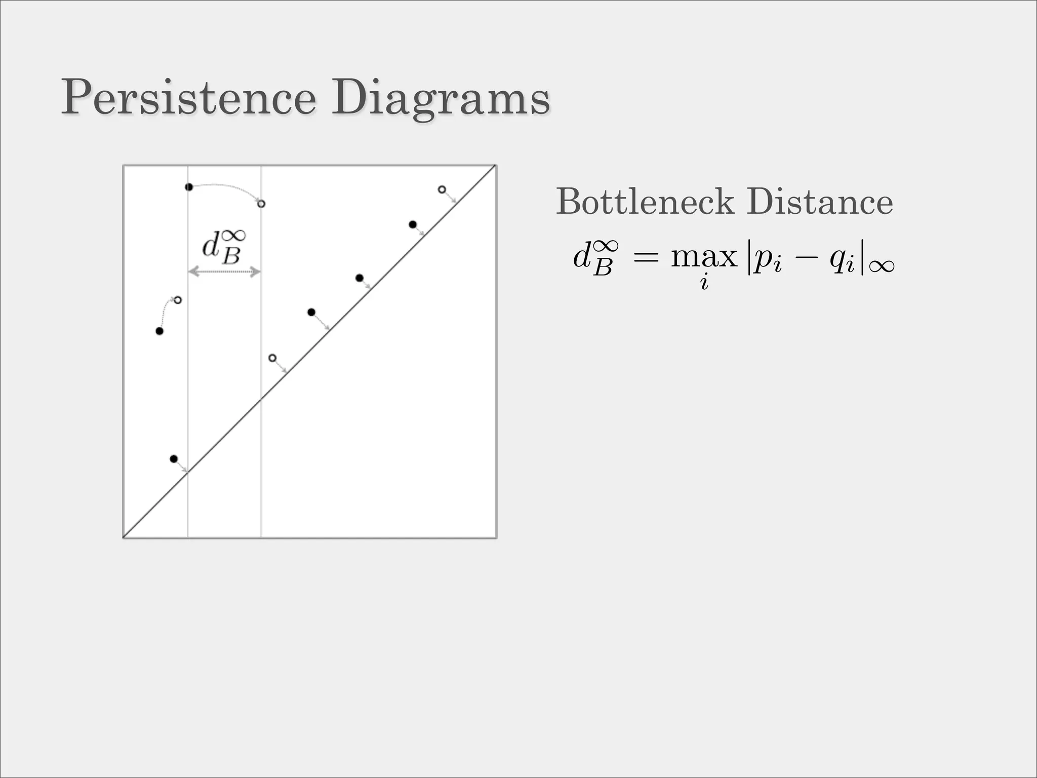
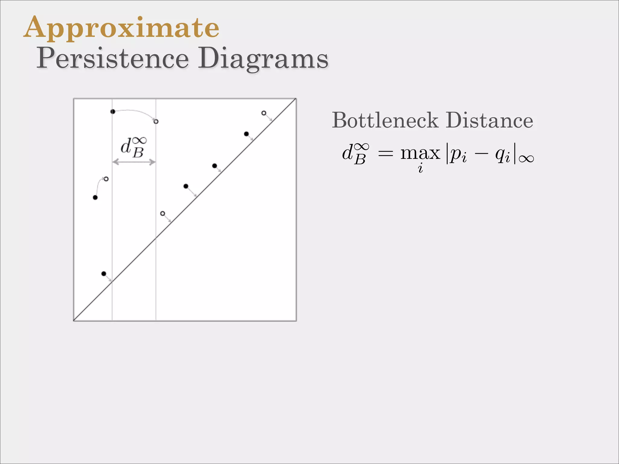
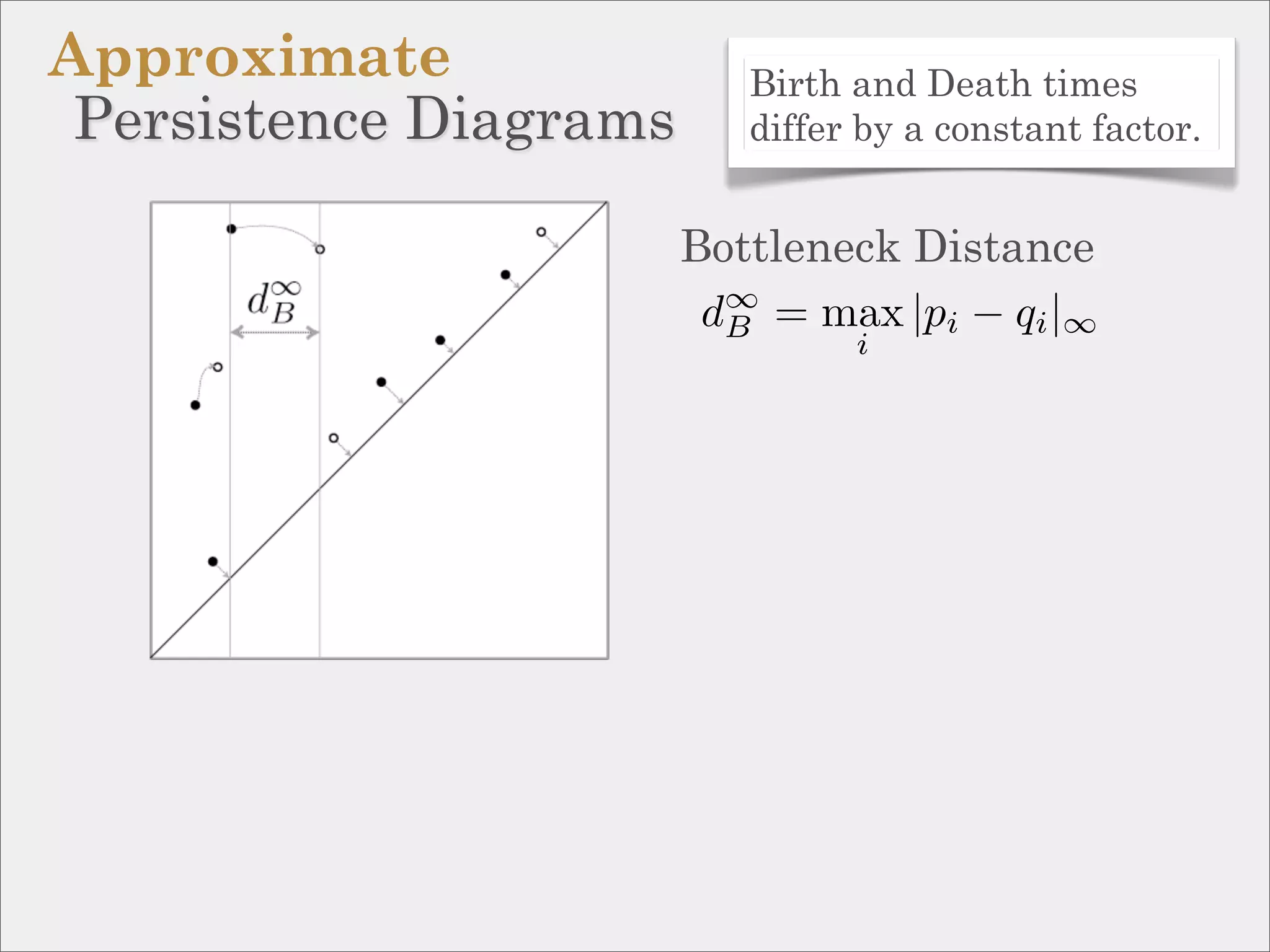
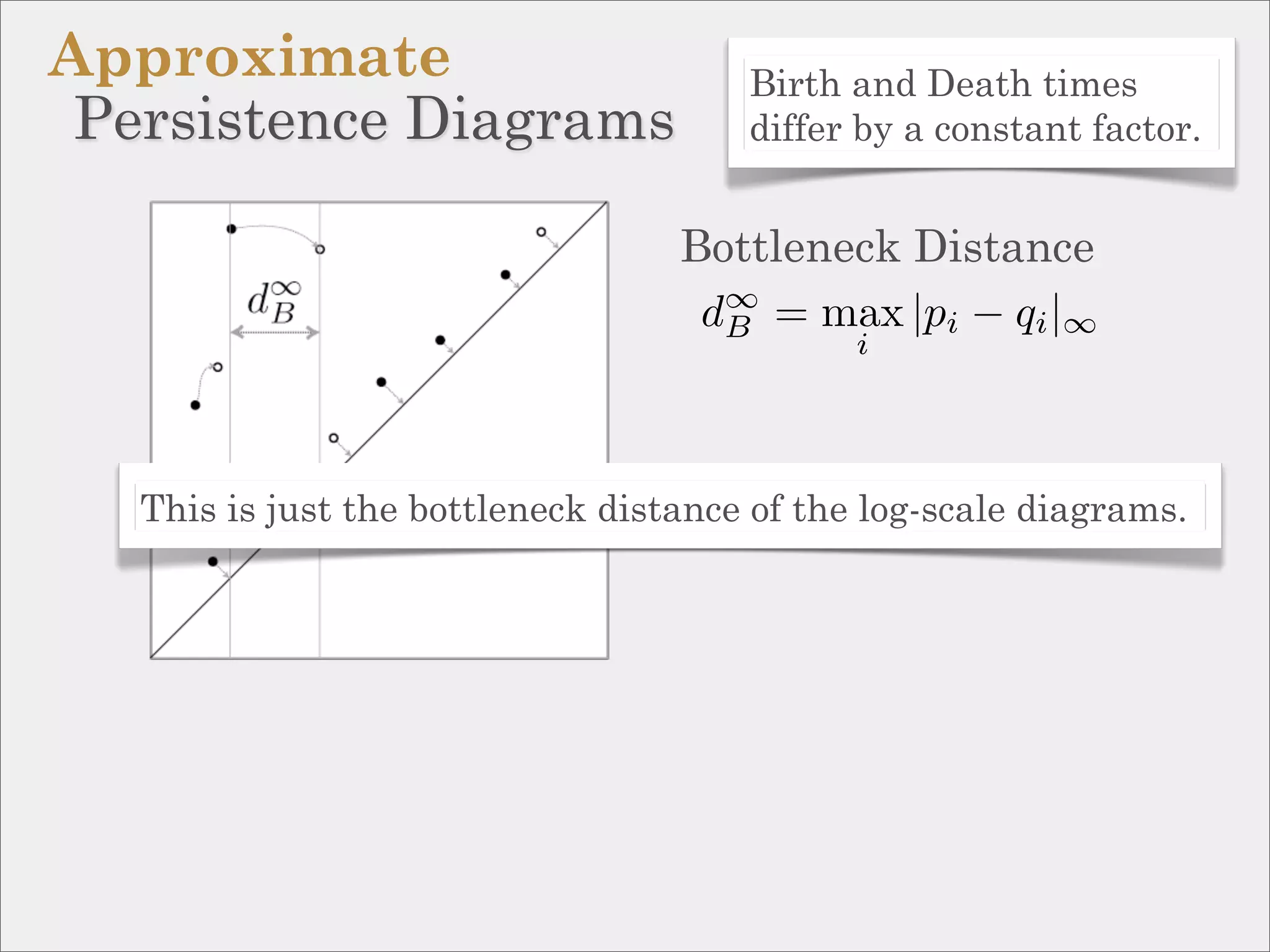
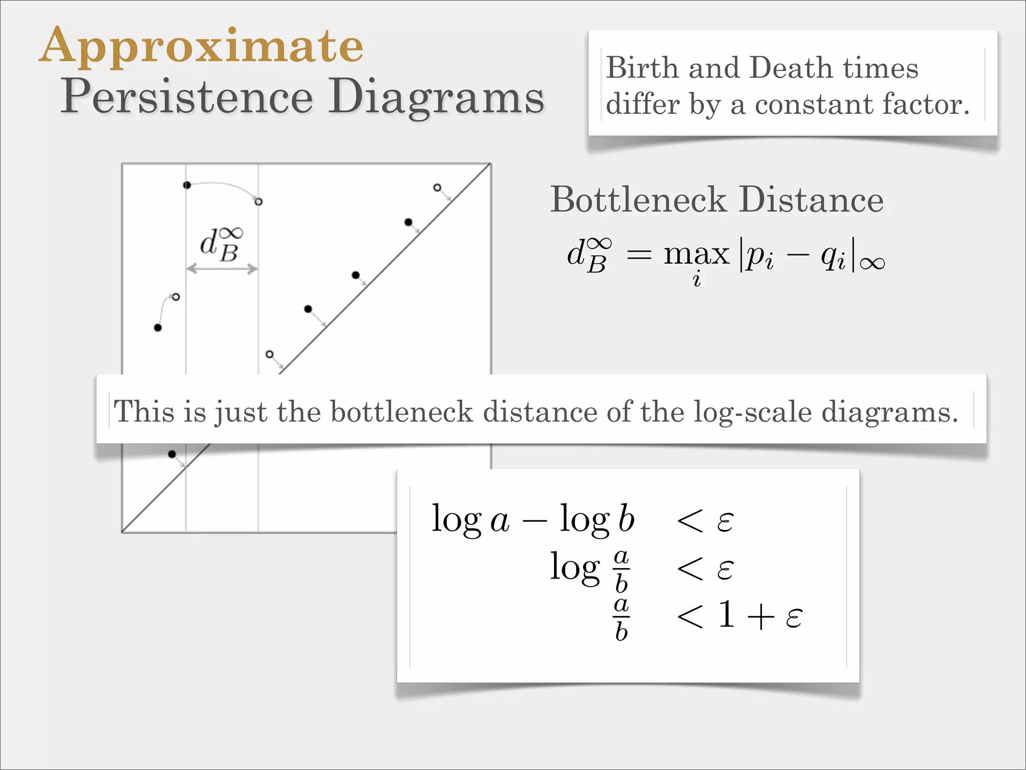
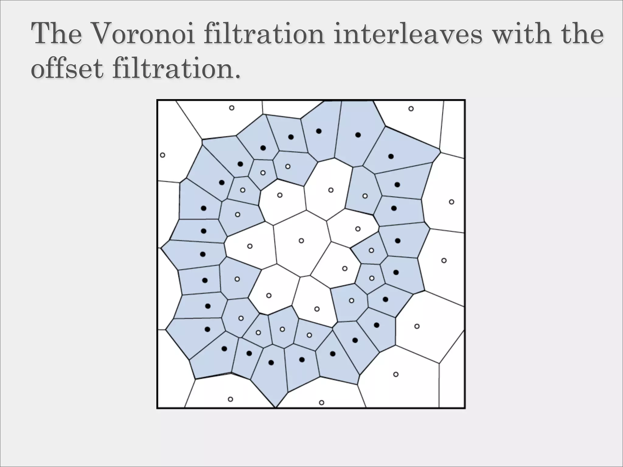
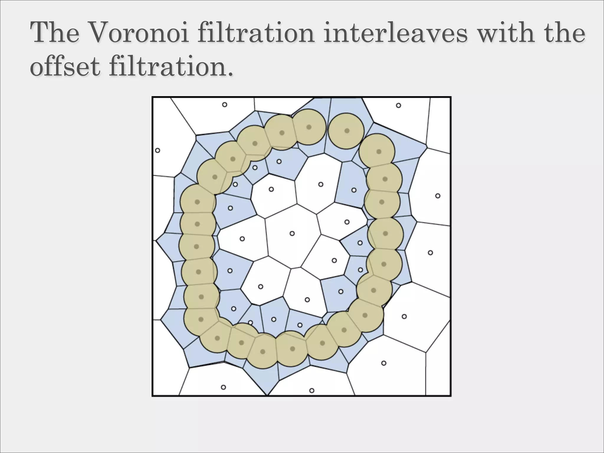
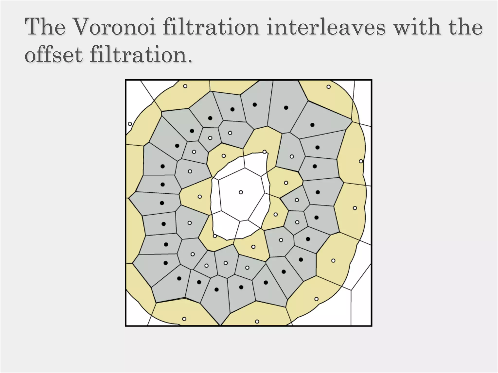
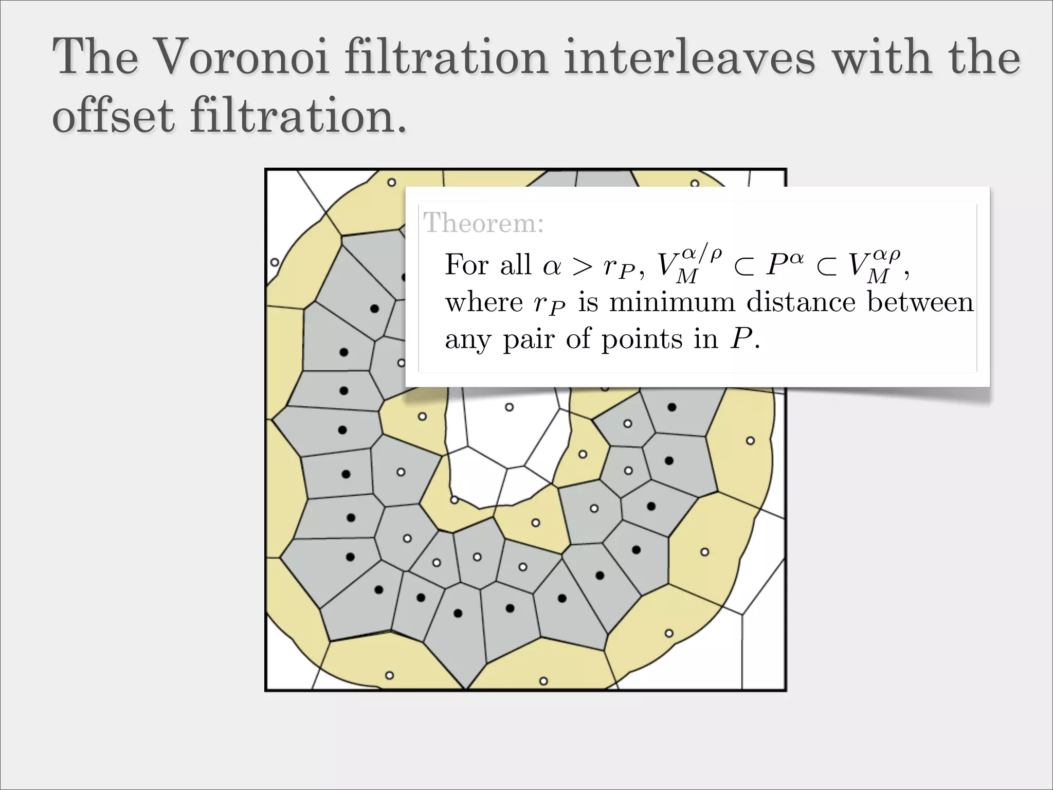
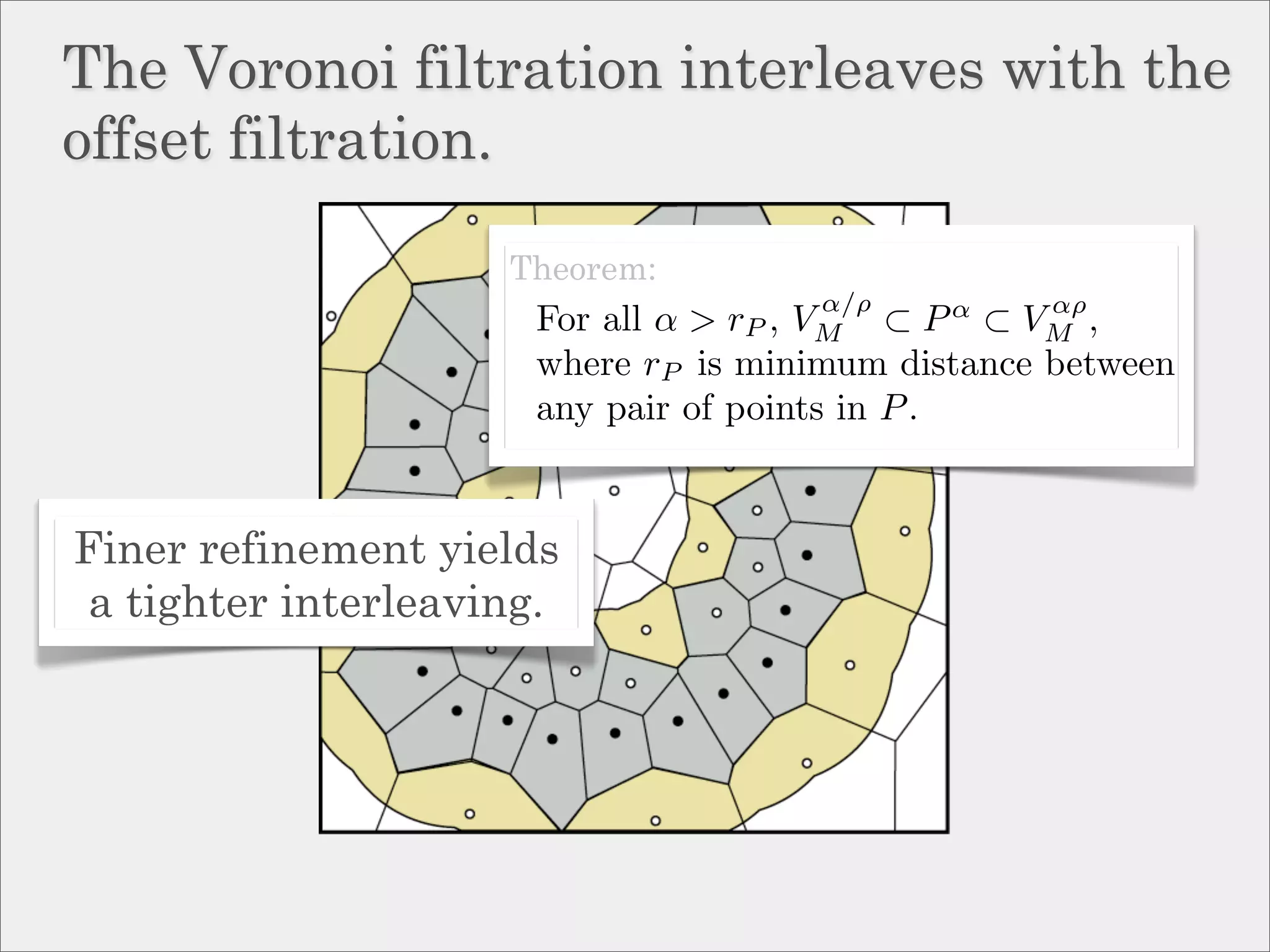
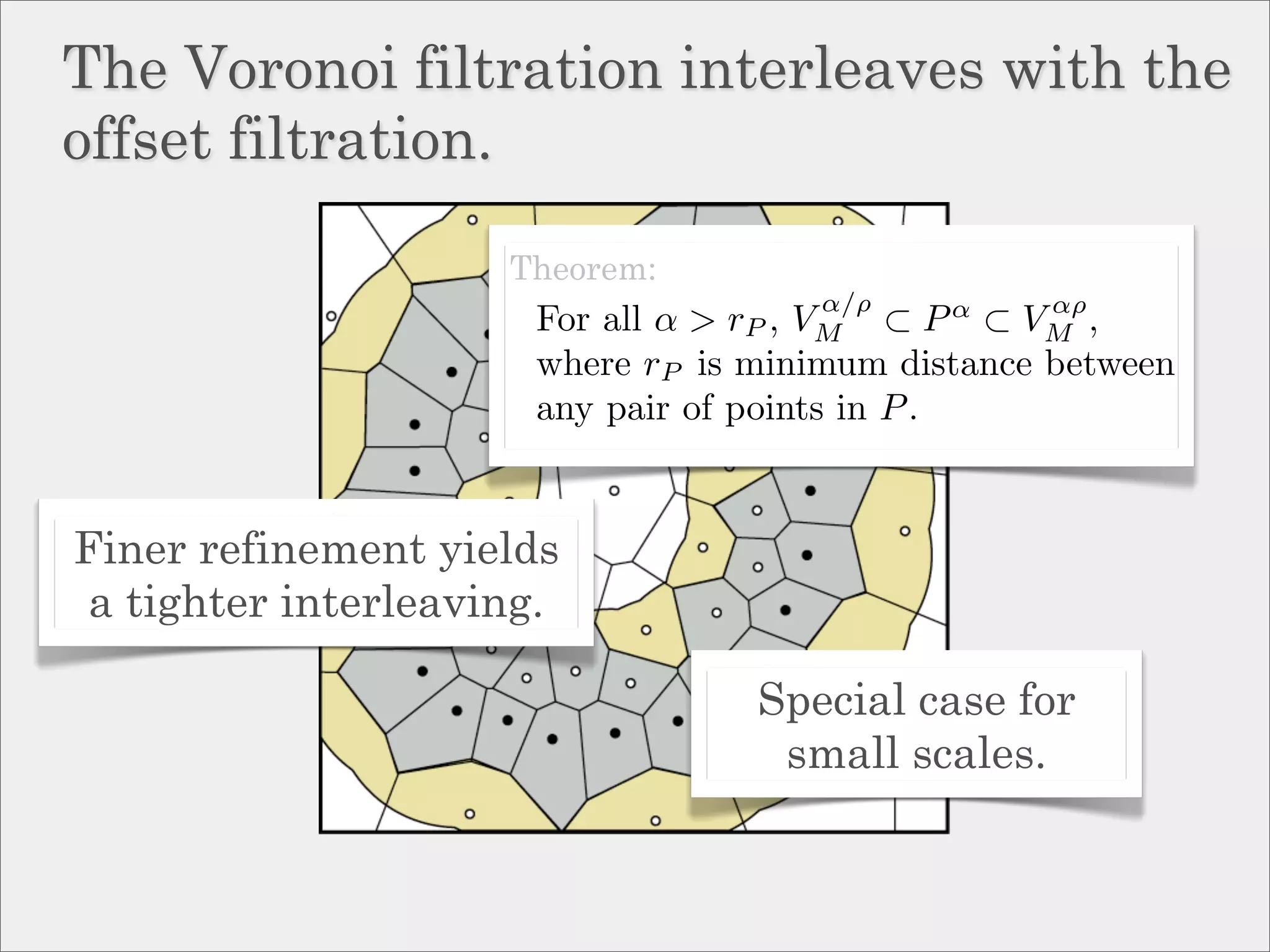
![Approximation via interleaving.
Definition:
Two filtrations, {Pα } and {Qα } are
ε-interleaved if Pα−ε ⊆ Qα ⊆ Pα+ε
for all α.
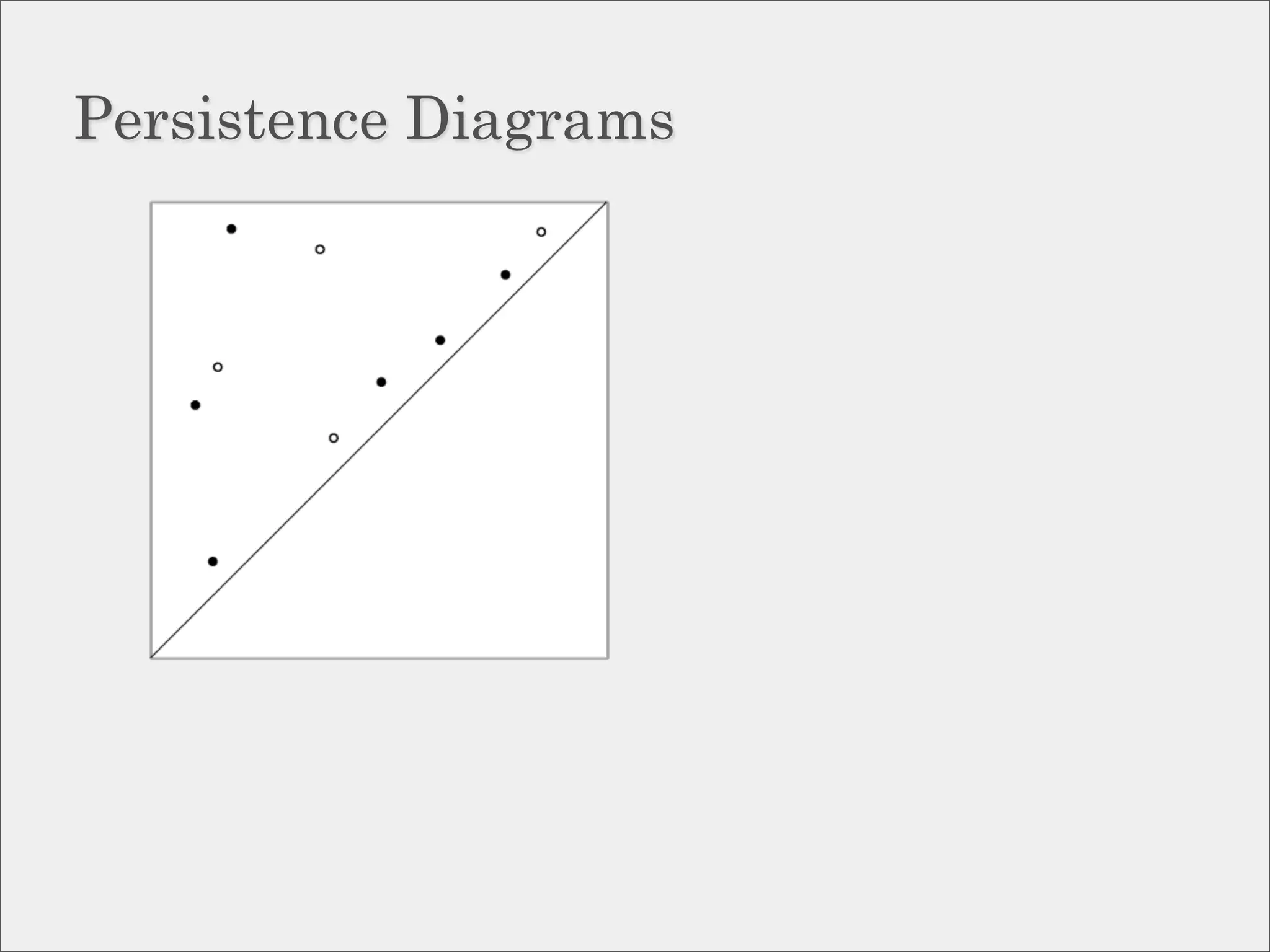
Theorem [Chazal et al, ’09]:
If {Pα } and {Qα } are ε-interleaved then
their persistence diagrams are ε-close in
the bottleneck distance.](https://image.slidesharecdn.com/socg10topological-100622141903-phpapp02/75/Topological-Inference-via-Meshing-50-2048.jpg)
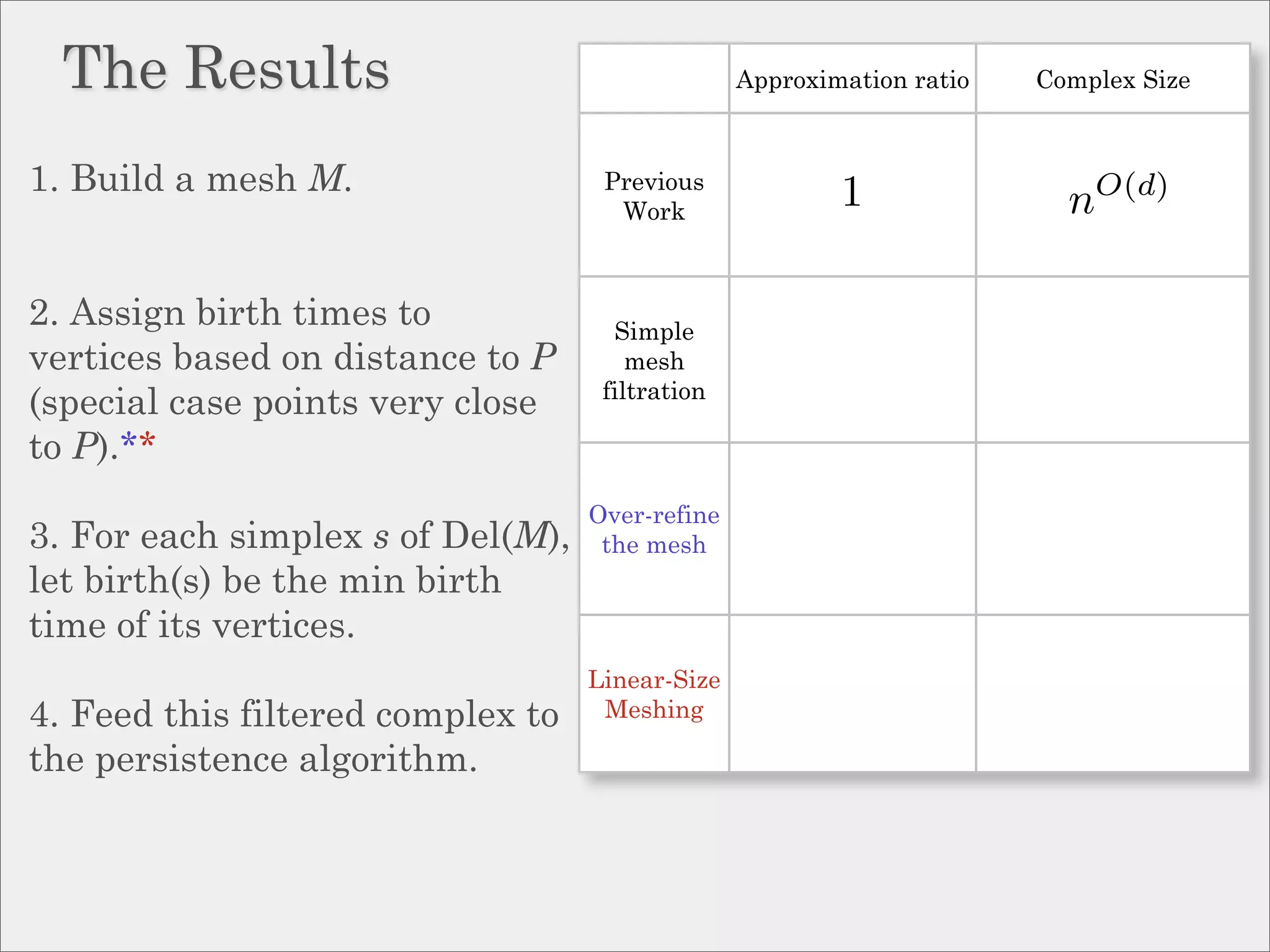
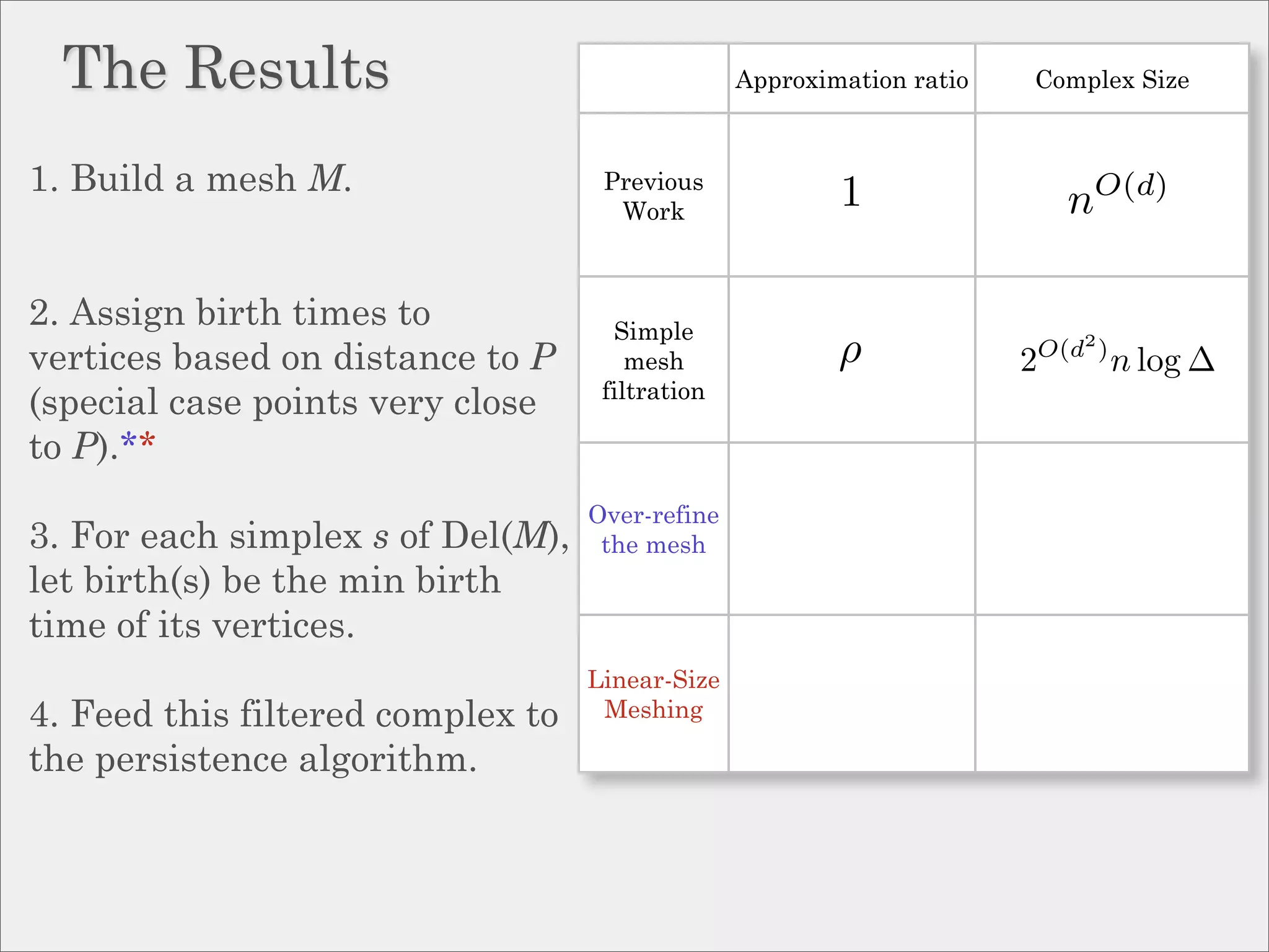
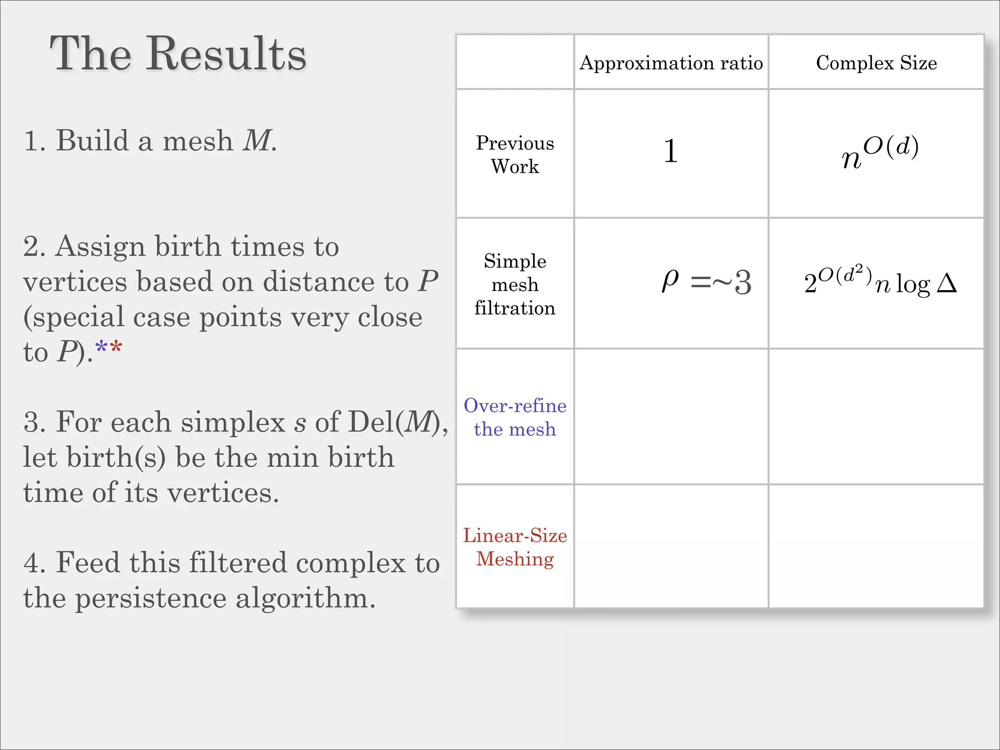
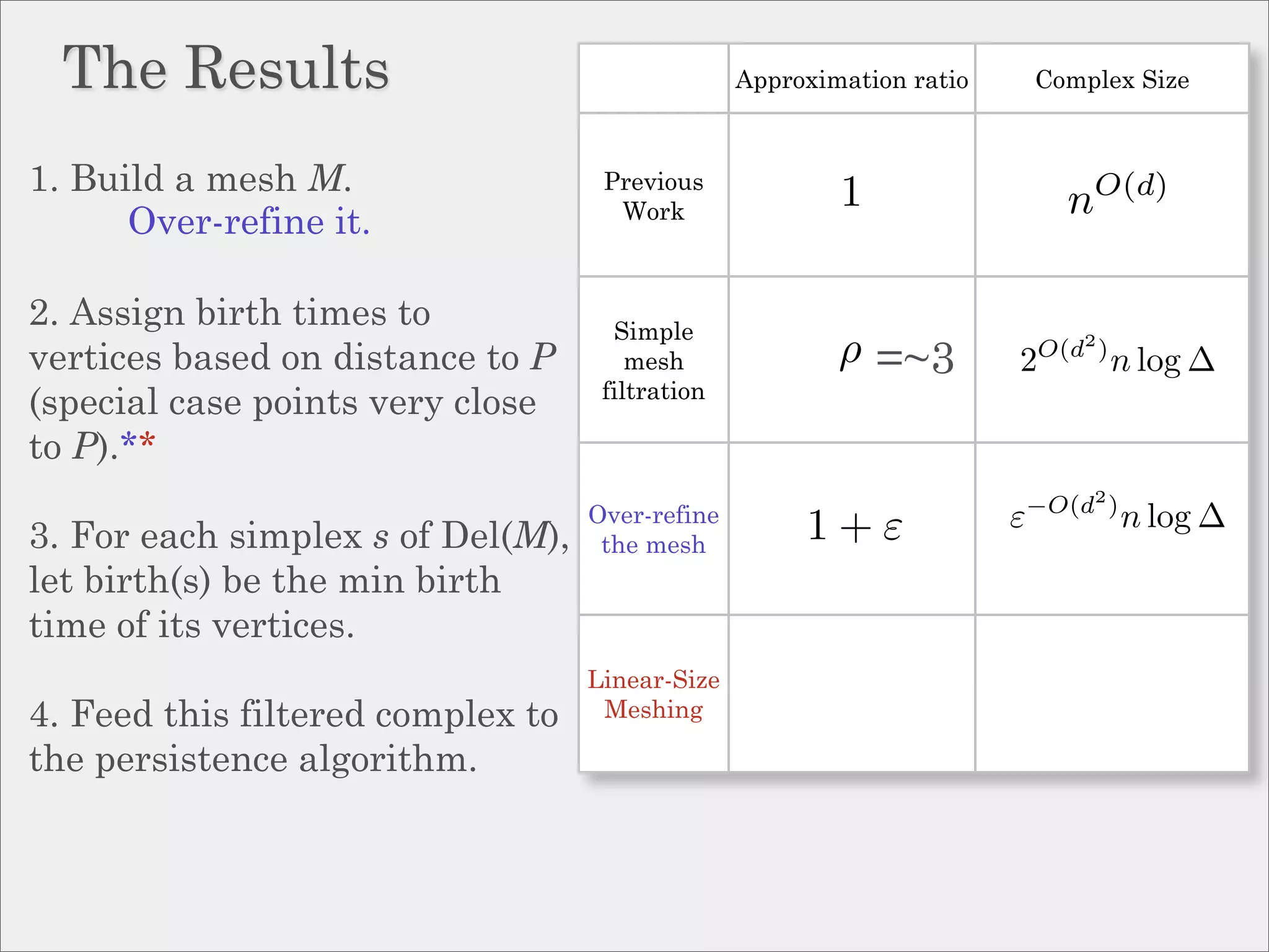
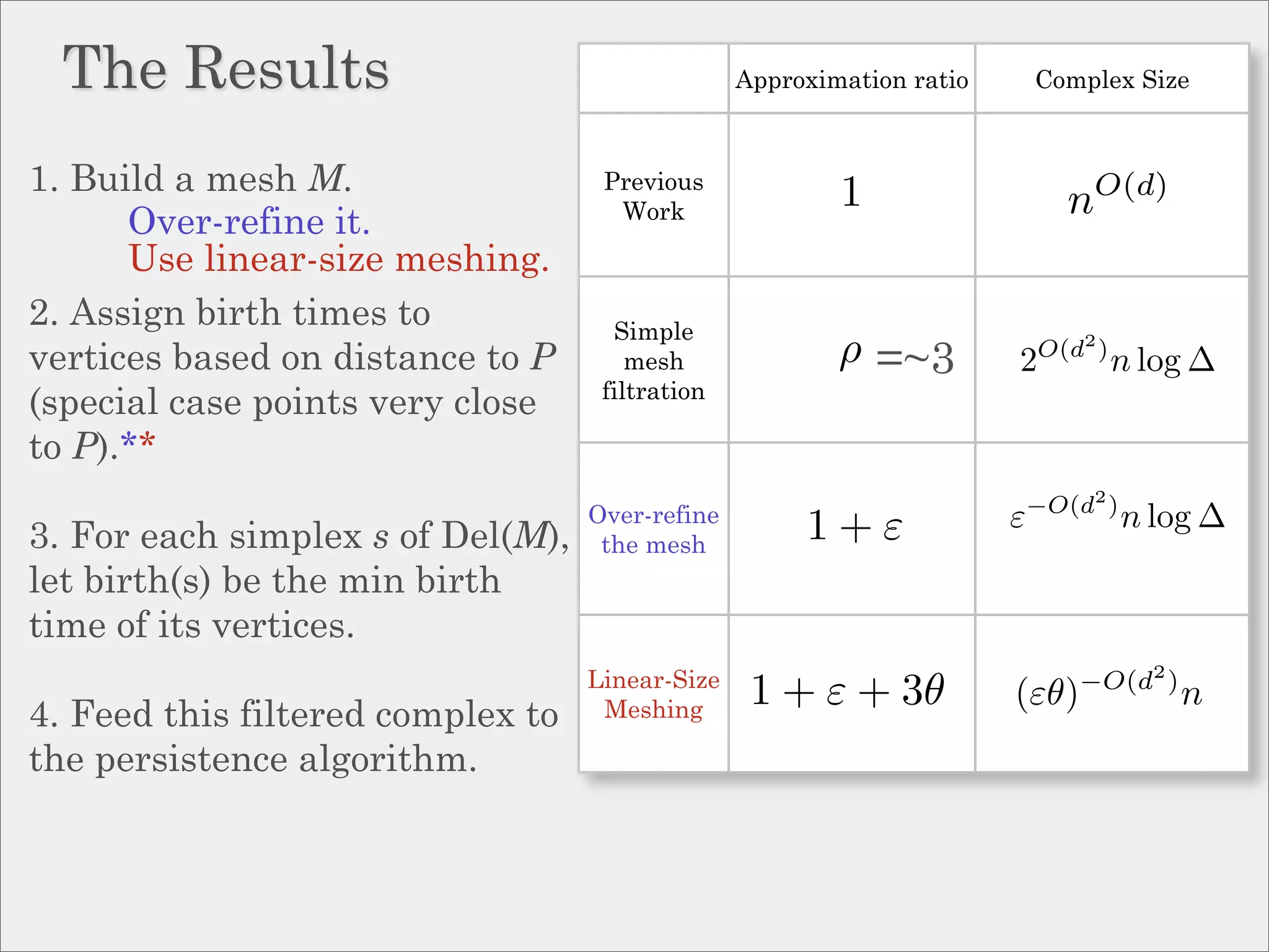


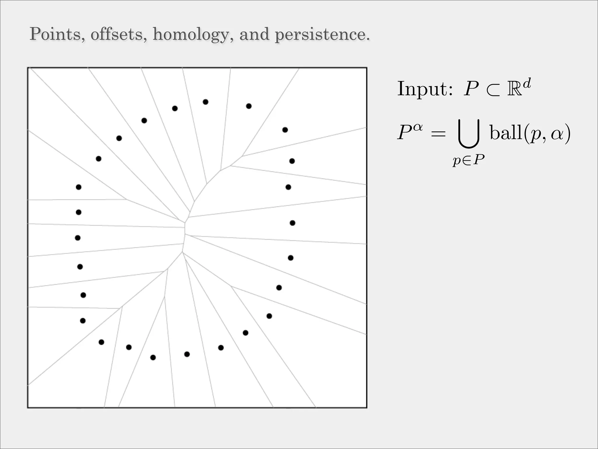
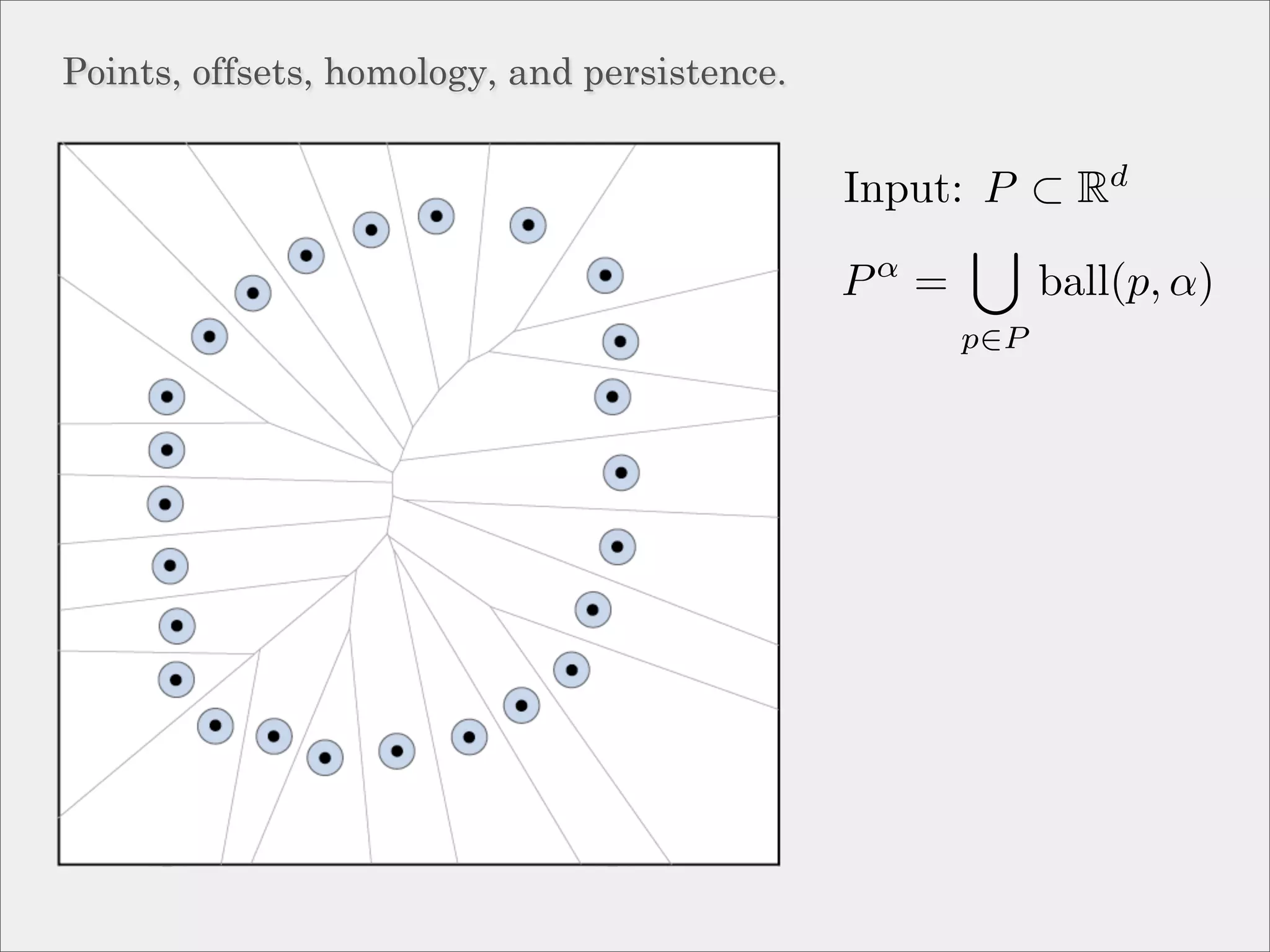
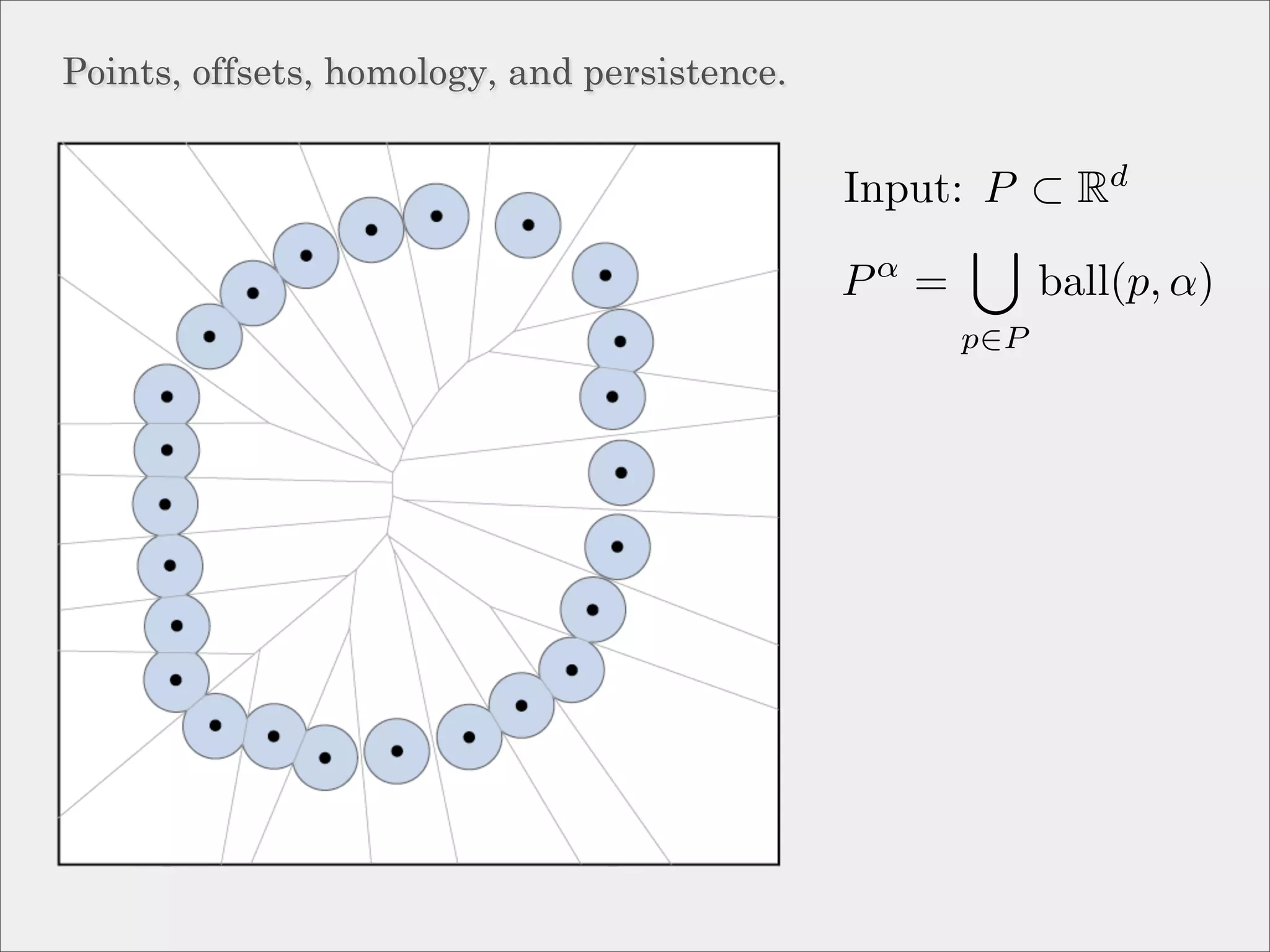
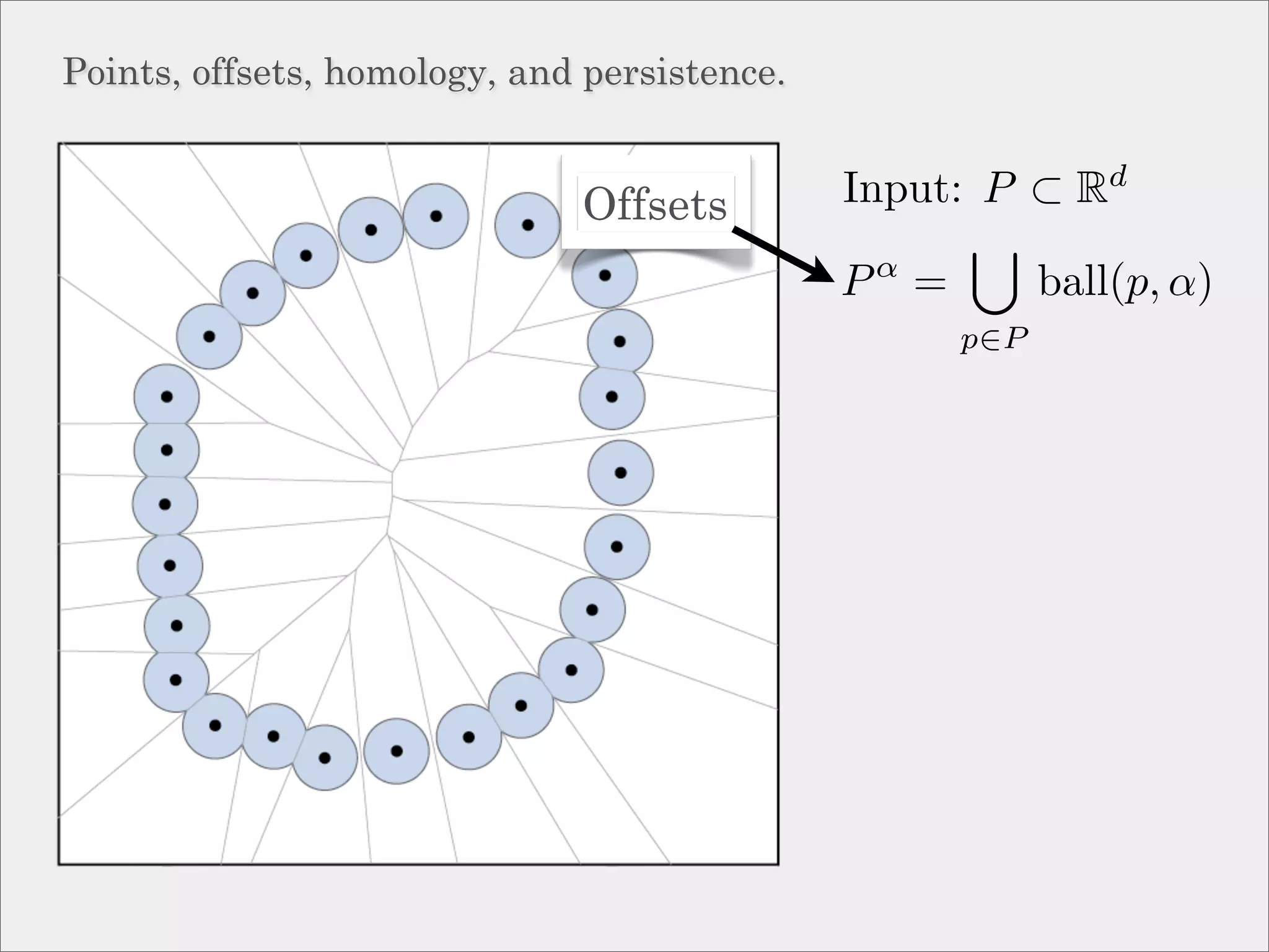
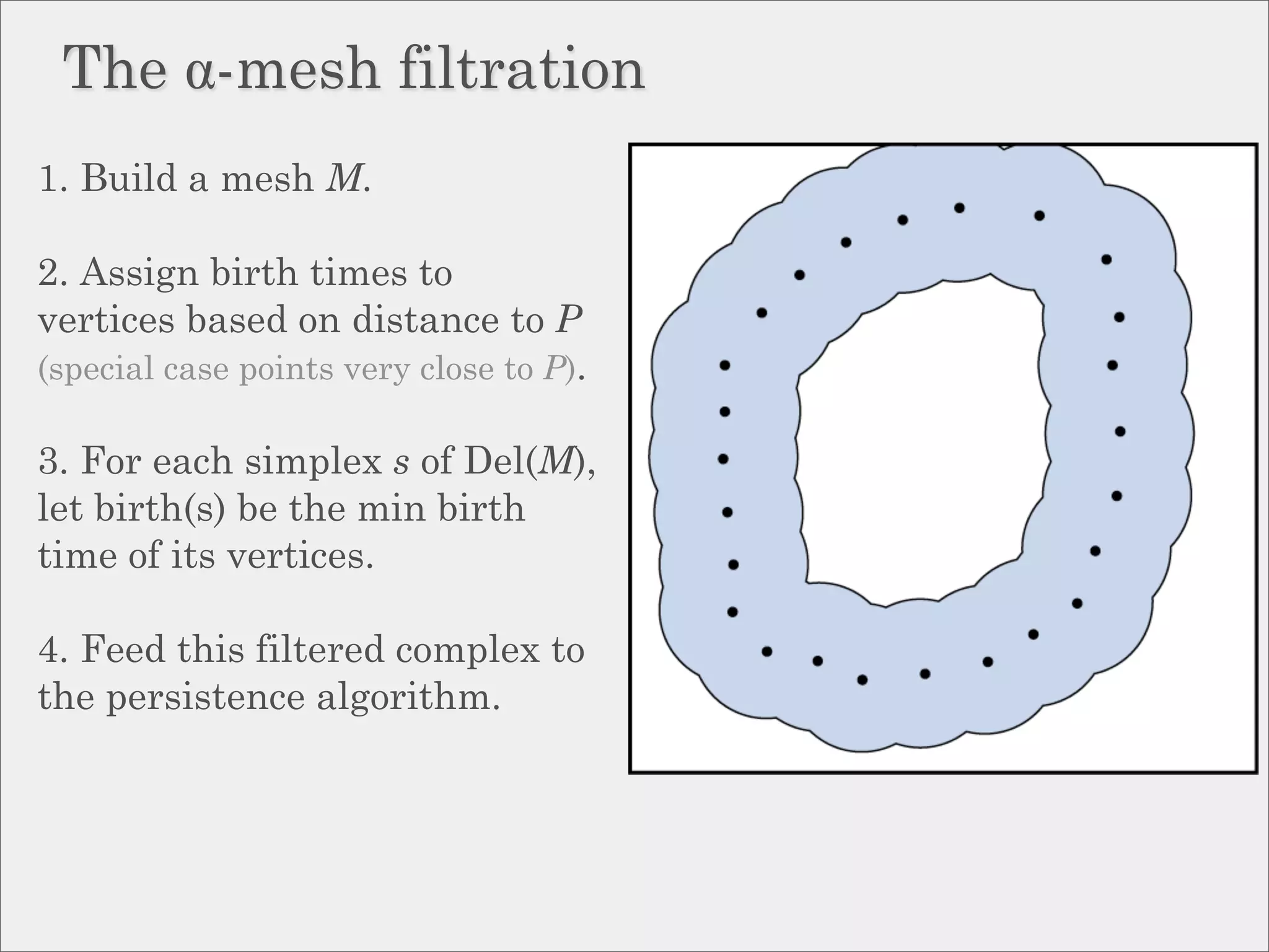
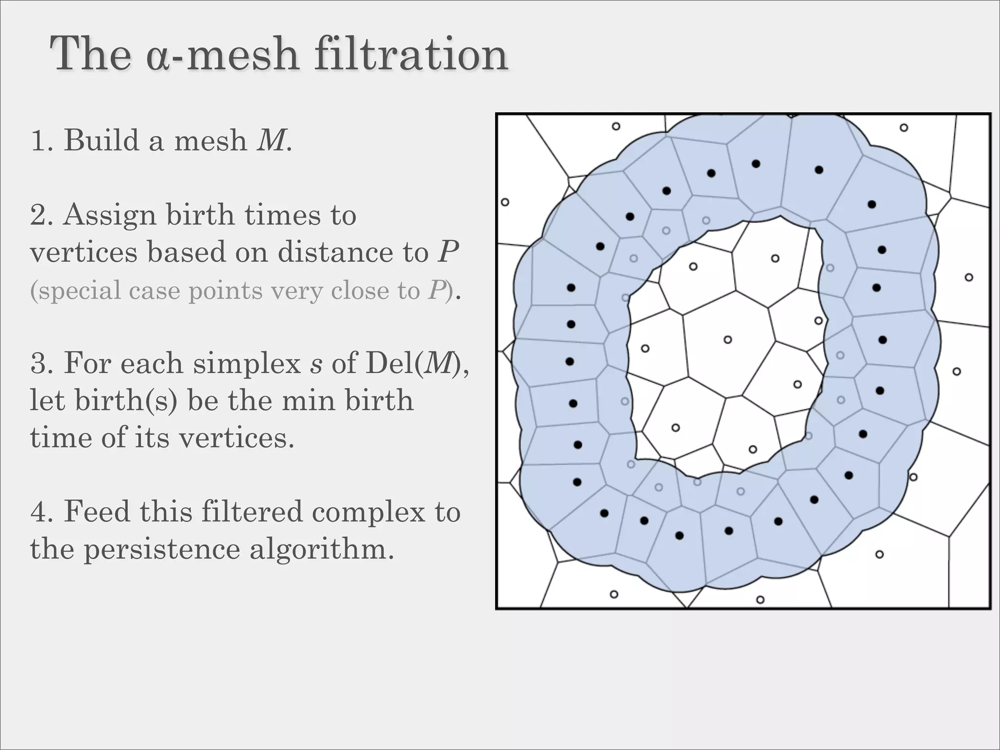
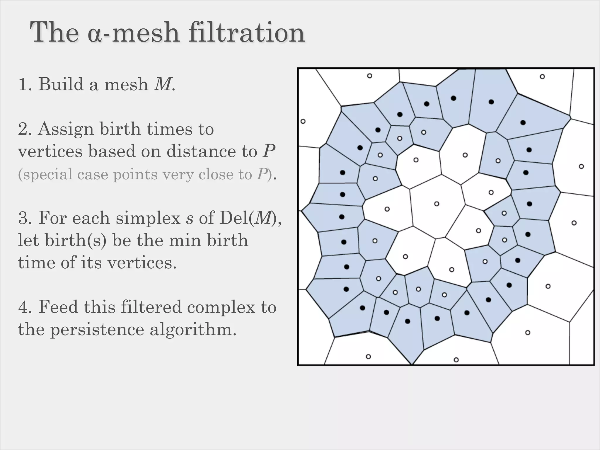
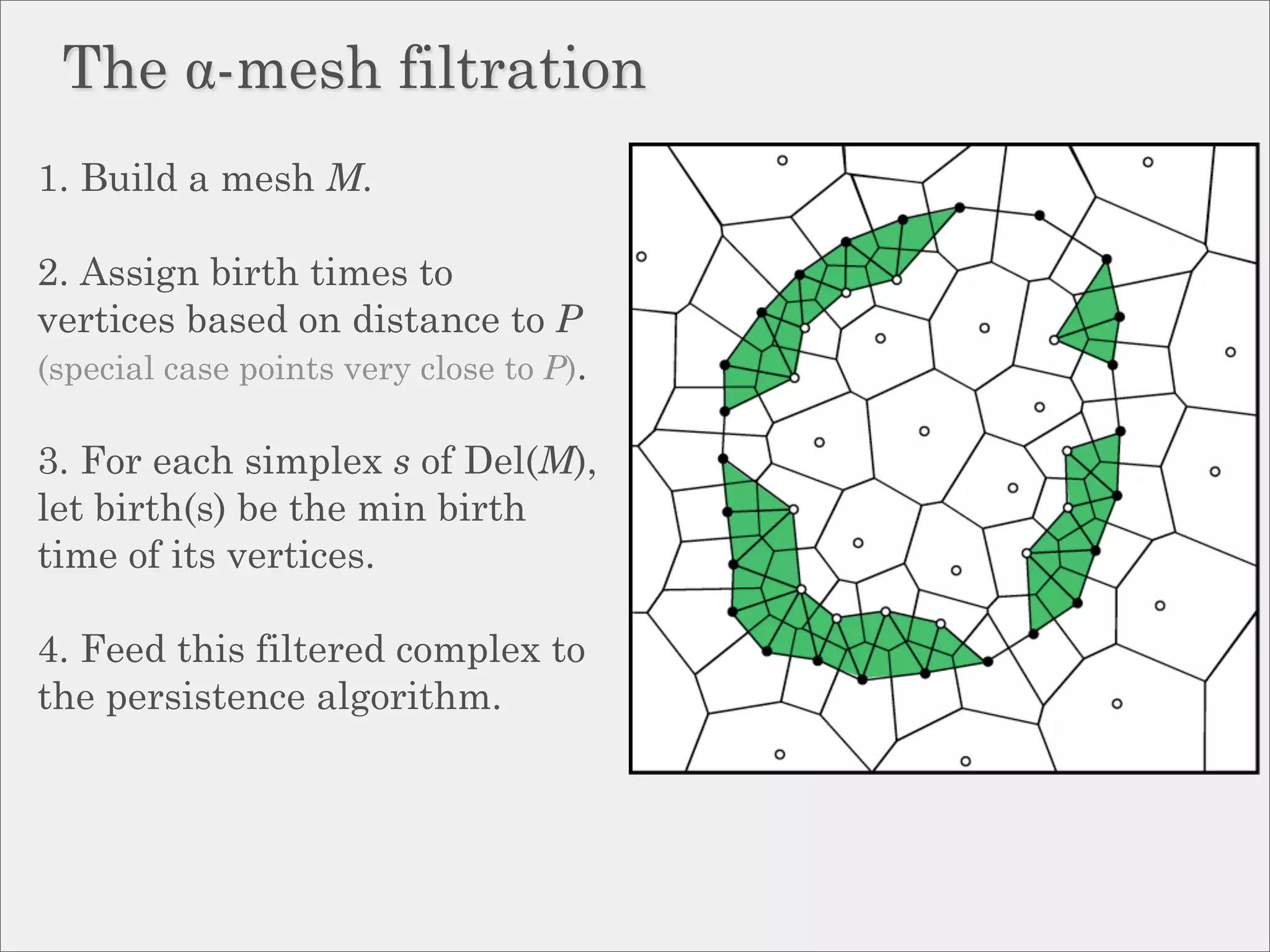
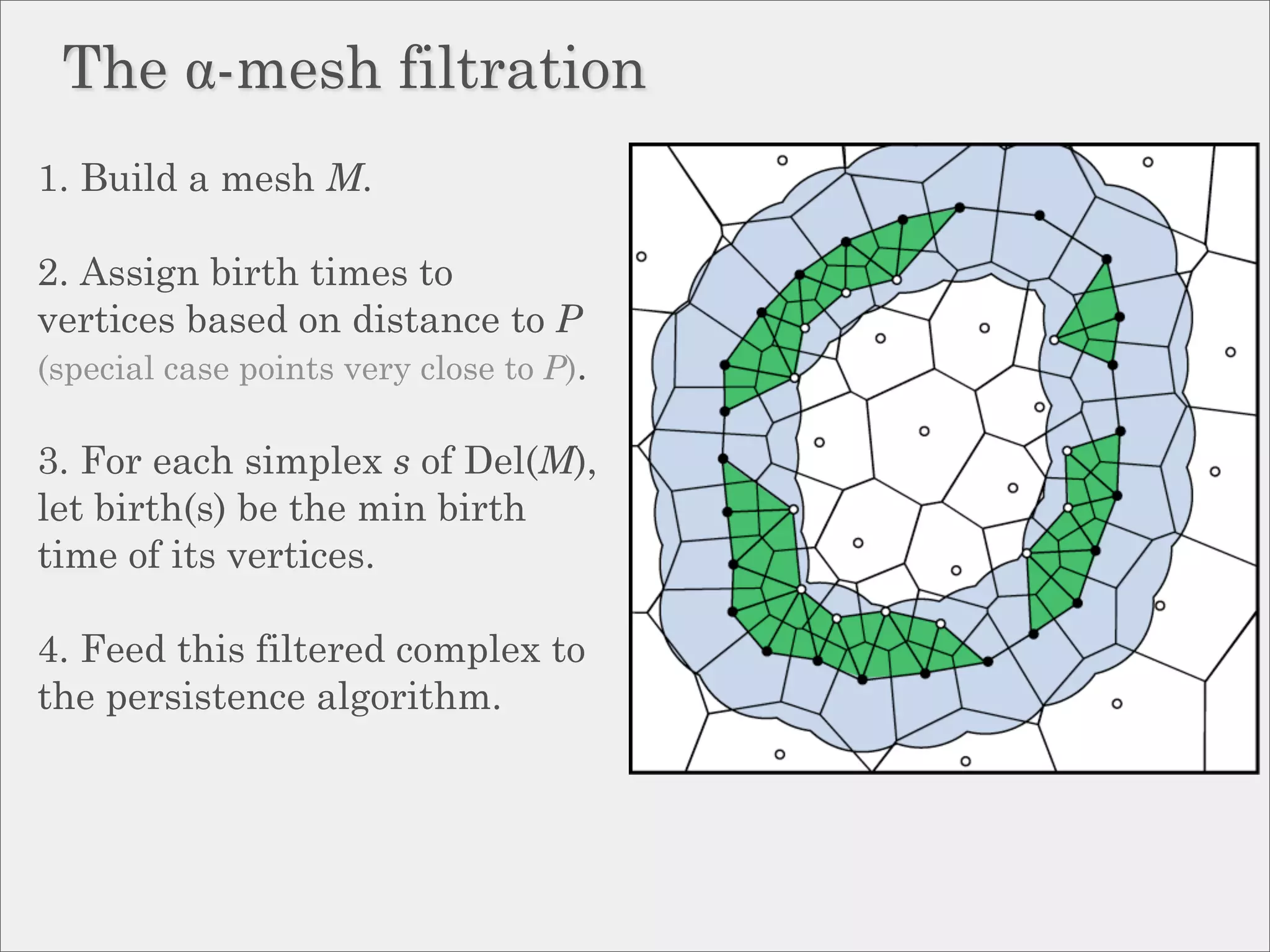
The document discusses topological inference through meshing, focusing on generating persistent homology from point data in Euclidean space. It reviews techniques for constructing meshes that can efficiently capture the object's topology, detailing geometric and topological phases, various filtration methods, and notable theorems regarding mesh quality and computational efficiency. Additionally, it addresses approximation strategies via interleaving to ensure close relationships between different filtrations.


![Coded Agents – with UiPath SDK + LangGraph [Virtual Hands-on Workshop]](https://cdn.slidesharecdn.com/ss_thumbnails/codedagentsdeck-251215155422-5497c599-thumbnail.jpg?width=640&height=640&fit=bounds)


