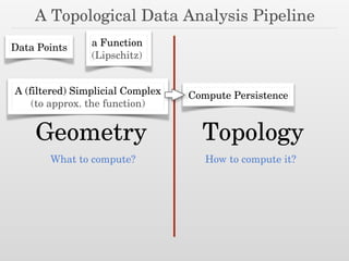
Download as PDF, PPTX


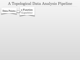


![The State of the Art
Asymptotics
“The Persistence Algorithm” [ELZ05] O(n3
)](https://image.slidesharecdn.com/fwcg13persistent-150202100454-conversion-gate01/85/Persistent-Homology-and-Nested-Dissection-21-320.jpg)
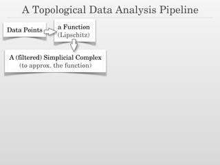
![The State of the Art
Asymptotics
“The Persistence Algorithm” [ELZ05]
via Matrix Multiplication [MMS11]
O(n3
)
O(n!
)](https://image.slidesharecdn.com/fwcg13persistent-150202100454-conversion-gate01/85/Persistent-Homology-and-Nested-Dissection-22-320.jpg)
![The State of the Art
Asymptotics
“The Persistence Algorithm” [ELZ05]
via Matrix Multiplication [MMS11]
Output-Sensitive [CK12] O(|D(1 ) |n2
)
O(n3
)
O(n!
)](https://image.slidesharecdn.com/fwcg13persistent-150202100454-conversion-gate01/85/Persistent-Homology-and-Nested-Dissection-23-320.jpg)
![The State of the Art
Asymptotics
Heuristics
“The Persistence Algorithm” [ELZ05]
via Matrix Multiplication [MMS11]
Output-Sensitive [CK12] O(|D(1 ) |n2
)
O(n3
)
O(n!
)](https://image.slidesharecdn.com/fwcg13persistent-150202100454-conversion-gate01/85/Persistent-Homology-and-Nested-Dissection-24-320.jpg)
![The State of the Art
Asymptotics
Heuristics
“The Persistence Algorithm” [ELZ05]
via Matrix Multiplication [MMS11]
Output-Sensitive [CK12]
Persistent Cohomology [MdSV-J11]
O(|D(1 ) |n2
)
O(n3
)
O(n!
)](https://image.slidesharecdn.com/fwcg13persistent-150202100454-conversion-gate01/85/Persistent-Homology-and-Nested-Dissection-25-320.jpg)
![The State of the Art
Asymptotics
Heuristics
“The Persistence Algorithm” [ELZ05]
via Matrix Multiplication [MMS11]
Output-Sensitive [CK12]
Persistent Cohomology [MdSV-J11]
Discrete Morse Reduction [MN13]
O(|D(1 ) |n2
)
O(n3
)
O(n!
)](https://image.slidesharecdn.com/fwcg13persistent-150202100454-conversion-gate01/85/Persistent-Homology-and-Nested-Dissection-26-320.jpg)
![The State of the Art
Asymptotics
Heuristics
“The Persistence Algorithm” [ELZ05]
via Matrix Multiplication [MMS11]
Output-Sensitive [CK12]
Persistent Cohomology [MdSV-J11]
Discrete Morse Reduction [MN13]
Clear and Compress [BKR13]
O(|D(1 ) |n2
)
O(n3
)
O(n!
)](https://image.slidesharecdn.com/fwcg13persistent-150202100454-conversion-gate01/85/Persistent-Homology-and-Nested-Dissection-27-320.jpg)
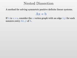

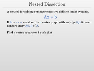
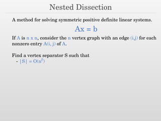
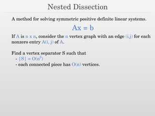
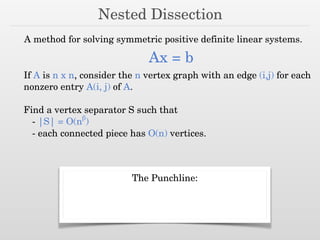
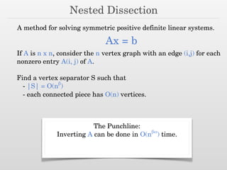
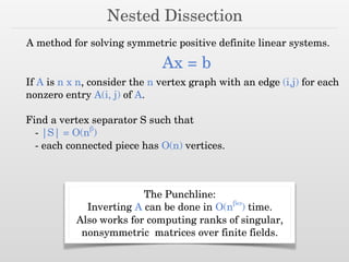
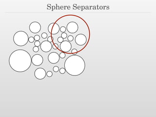
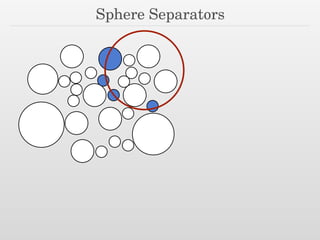
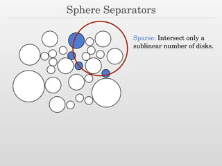
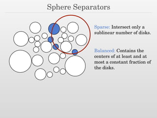
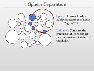
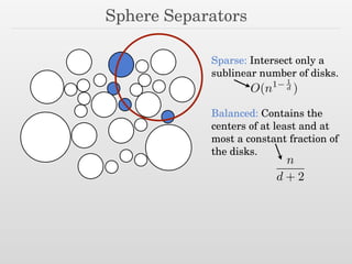


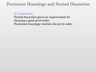
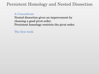

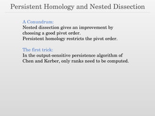
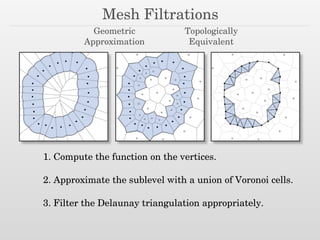
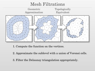
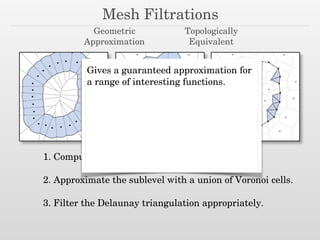

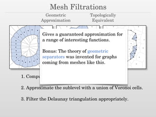

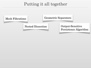
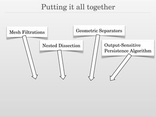
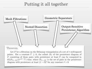


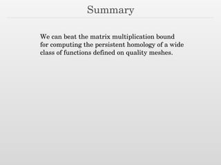
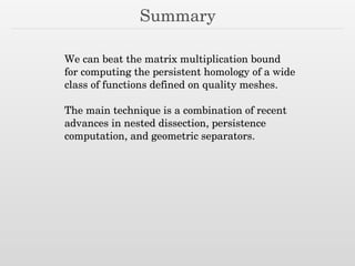


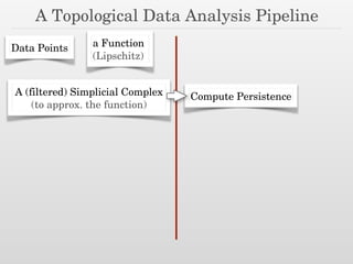
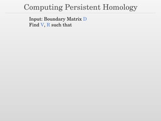
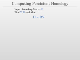
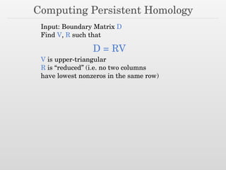
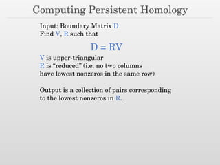
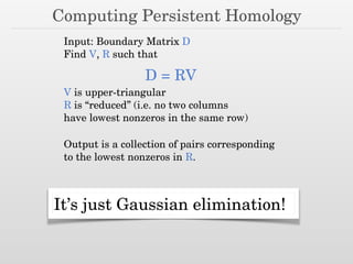
The document discusses using nested dissection and geometric separators to speed up computations of persistent homology. It proposes combining mesh filtrations, geometric separators, nested dissection, and output-sensitive persistence algorithms. This would allow beating the matrix multiplication time bound for computing persistent homology of functions defined on well-spaced point clouds. The technique exploits properties of meshes and separators to allow choosing a pivot order that improves the computation time.


![Polymer [ बहुलक ] Chemistry Notes PDF - Irfanullah Mehar - JJ Sir Chemistry.pdf](https://cdn.slidesharecdn.com/ss_thumbnails/polymerchemistrynotespdf-irfanullahmehar-jjsirchemistry-260210172118-3f9b37f7-thumbnail.jpg?width=640&height=640&fit=bounds)


