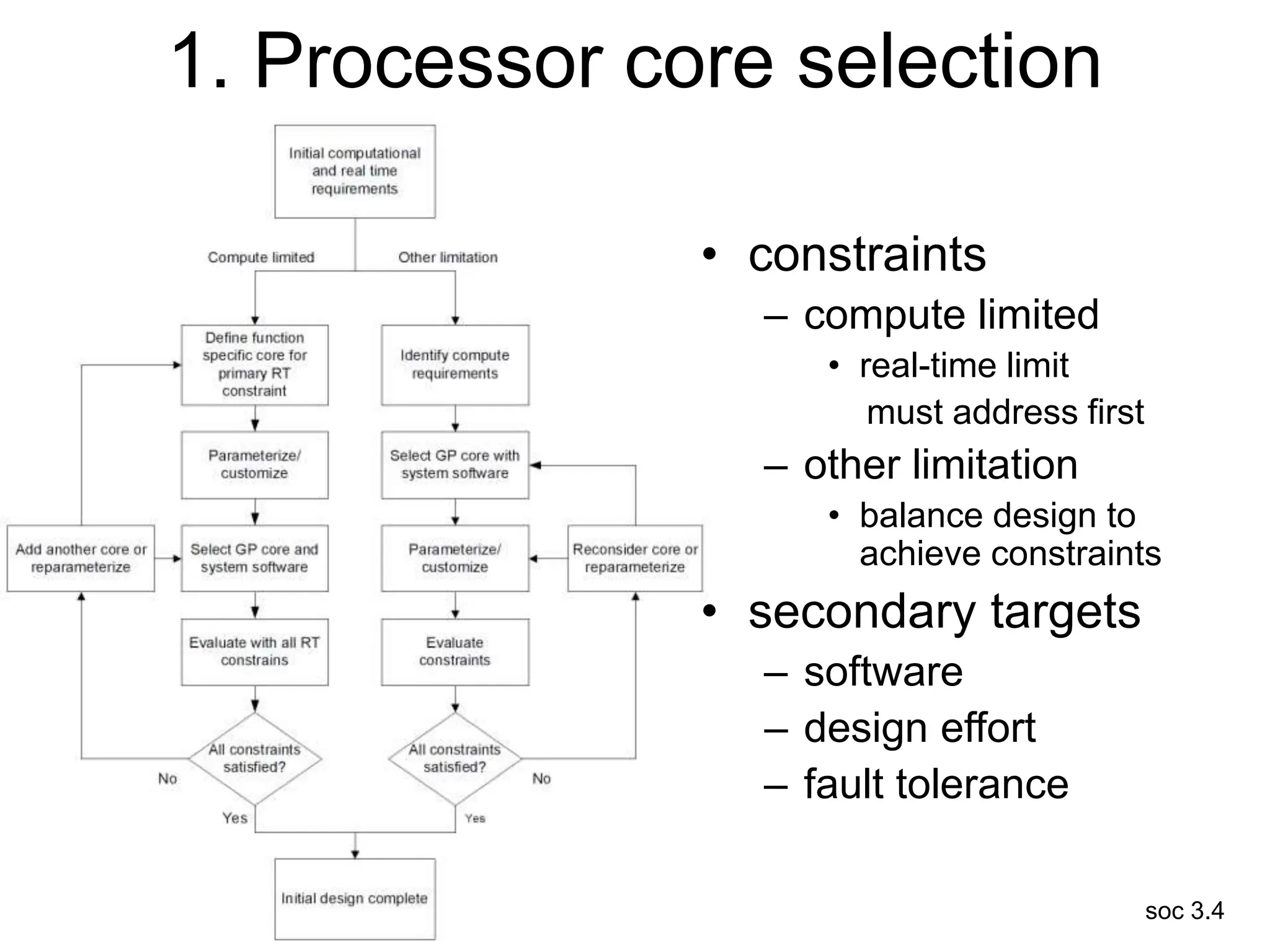
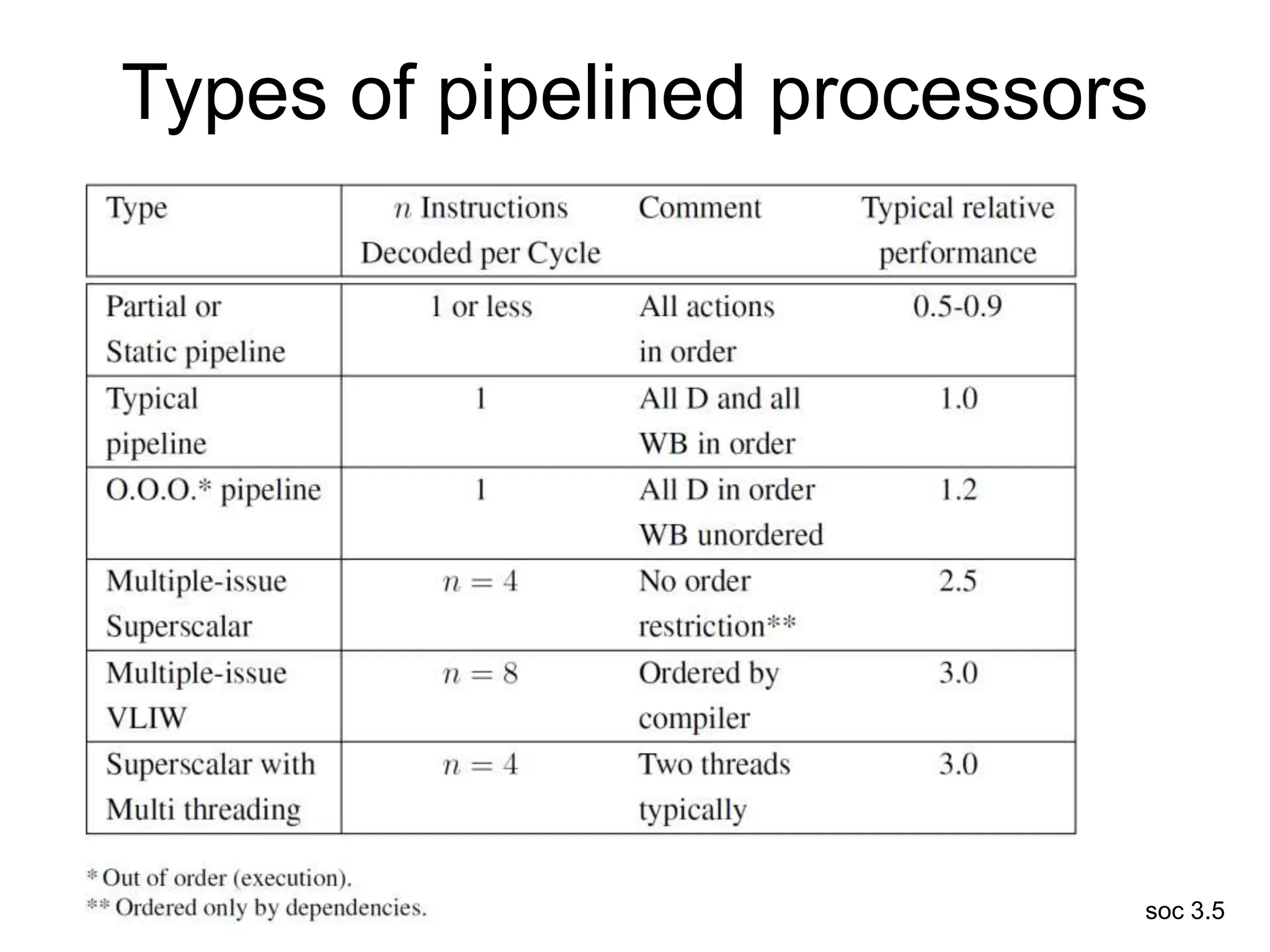
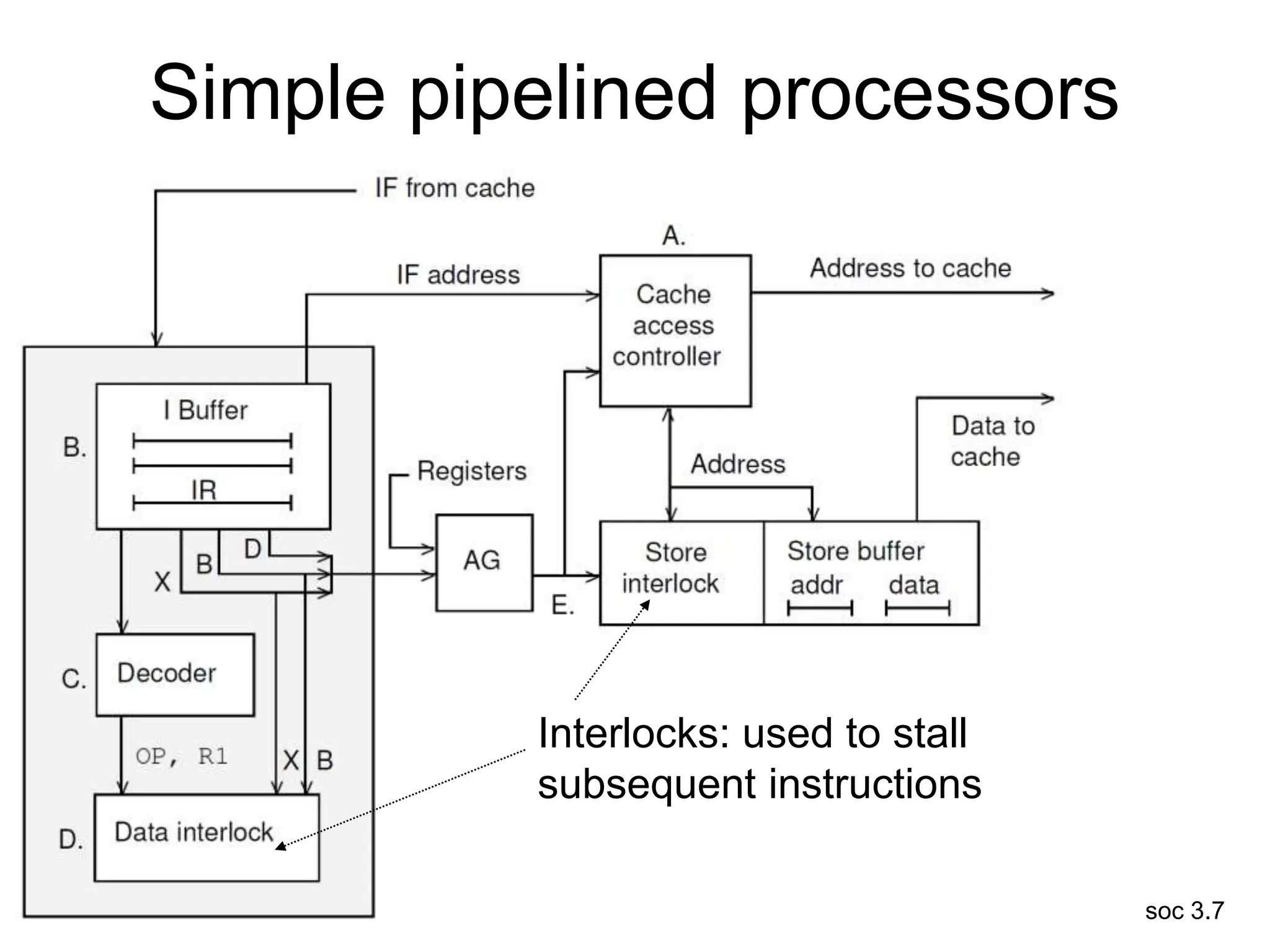
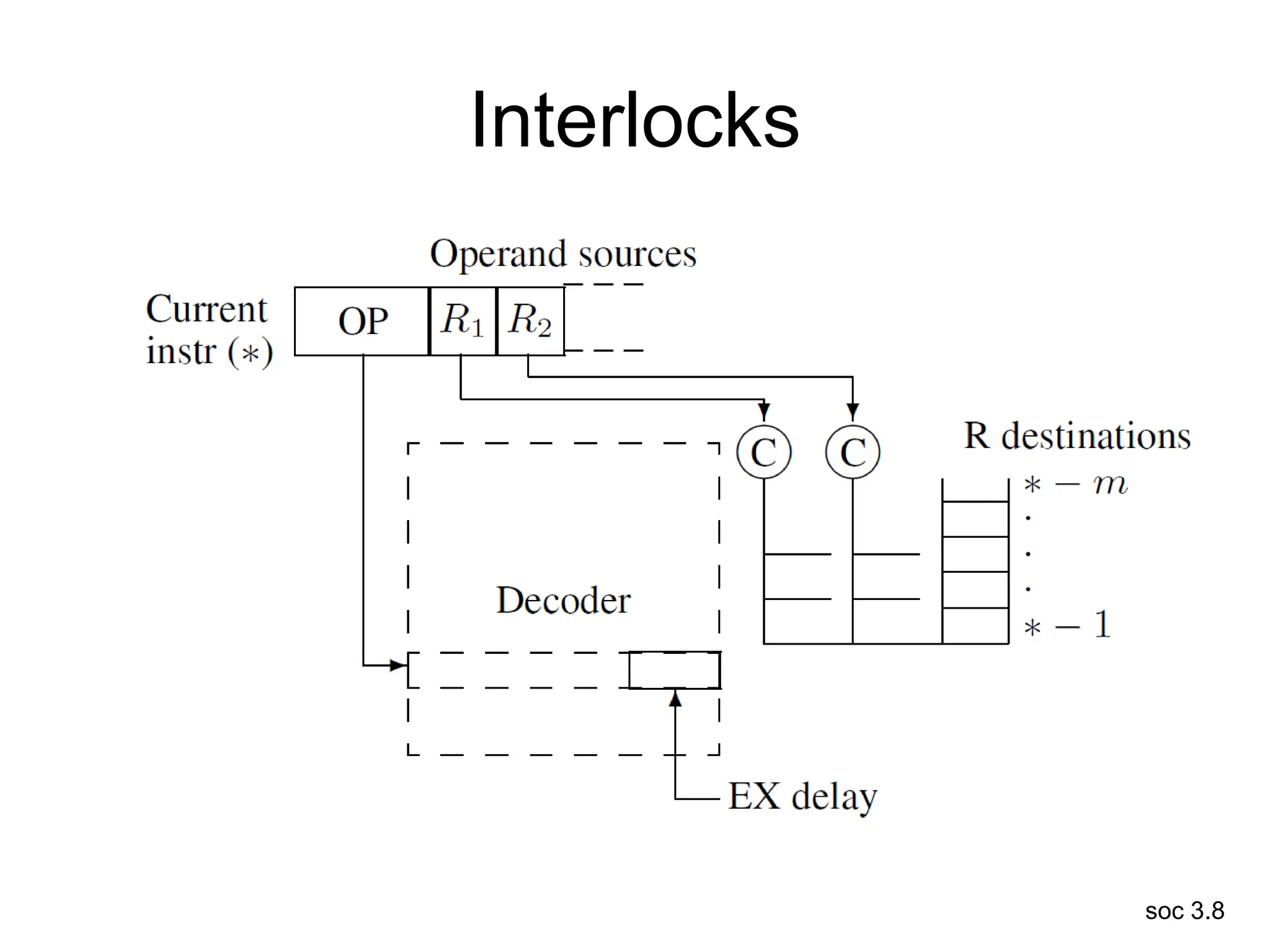
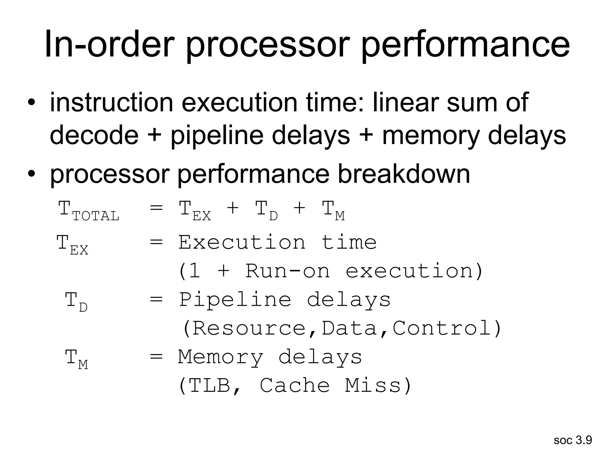
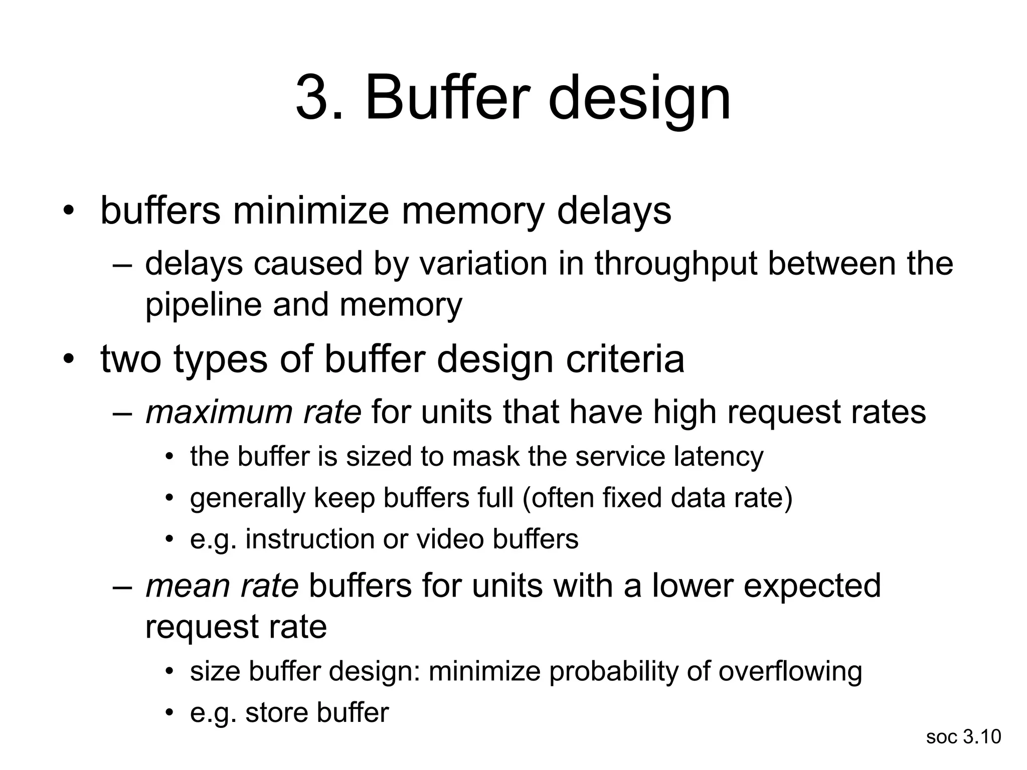
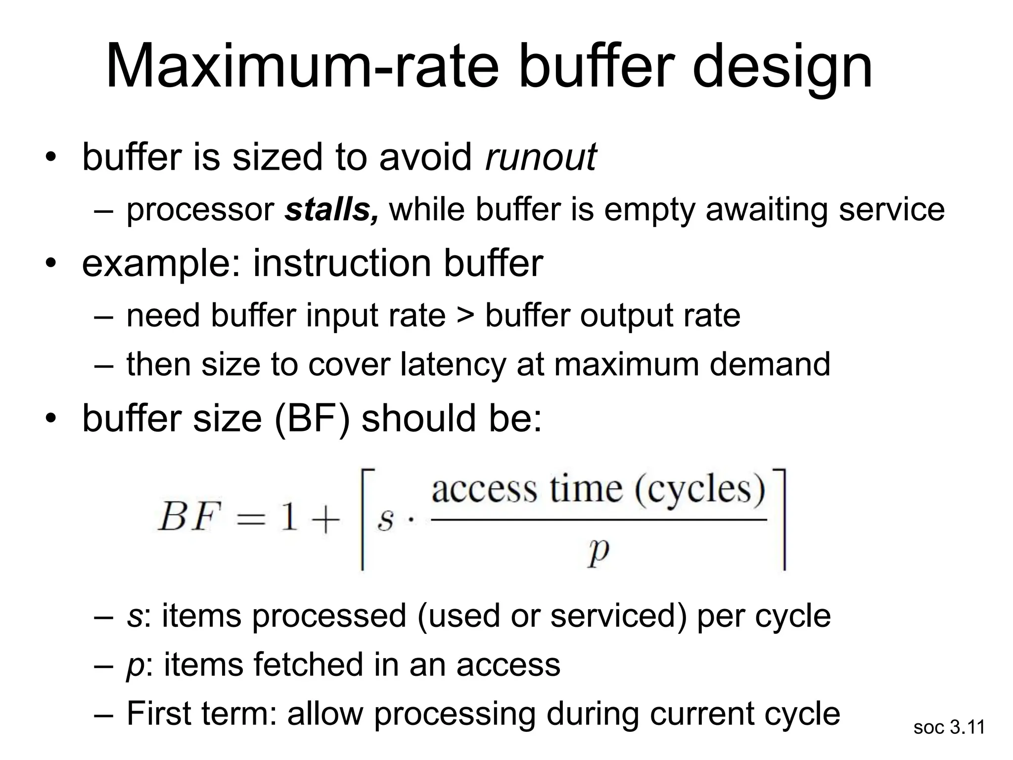
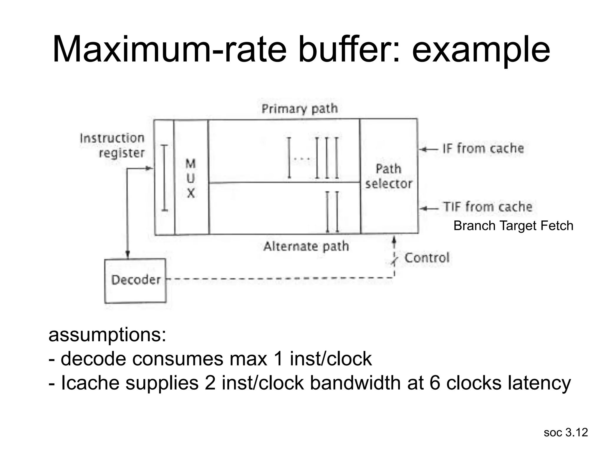
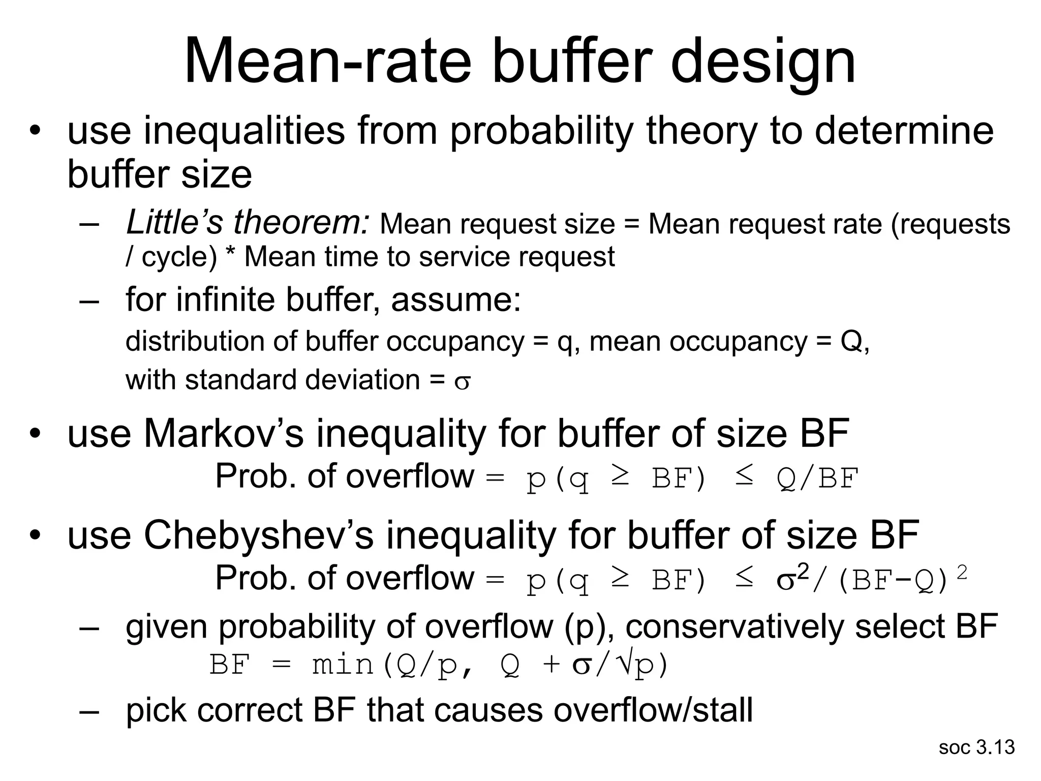
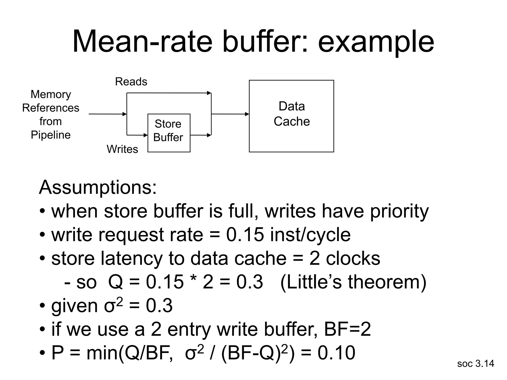
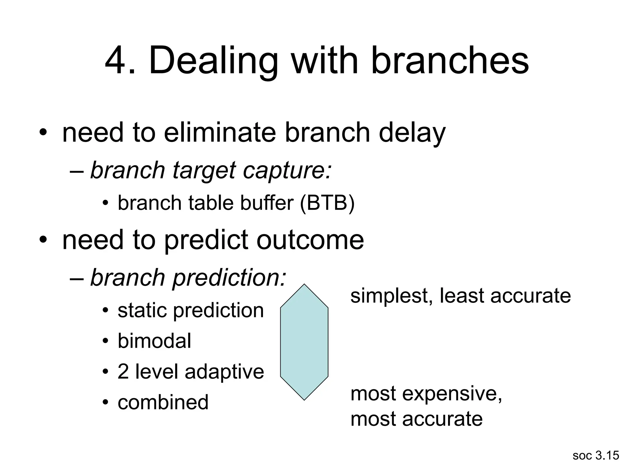
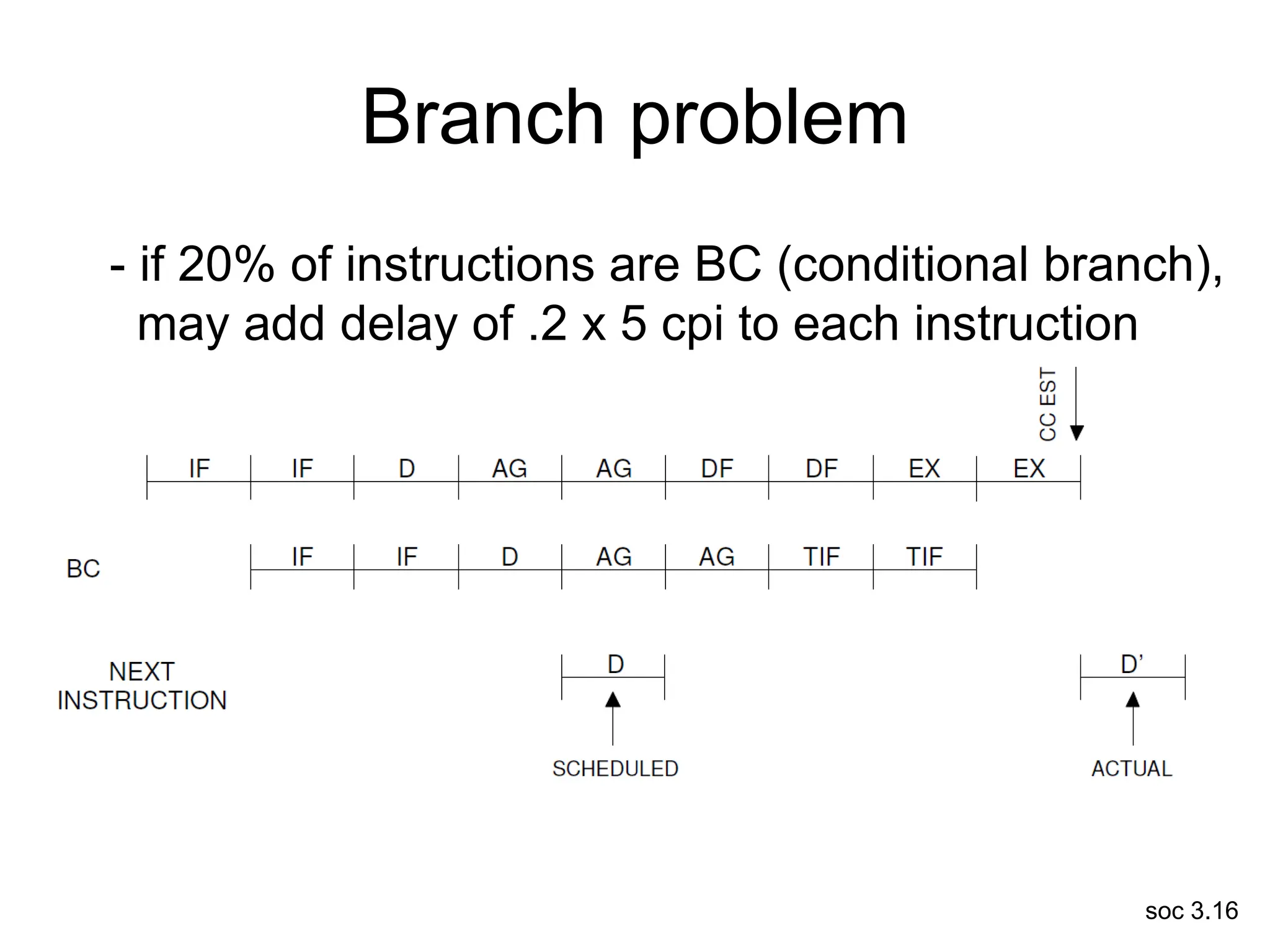
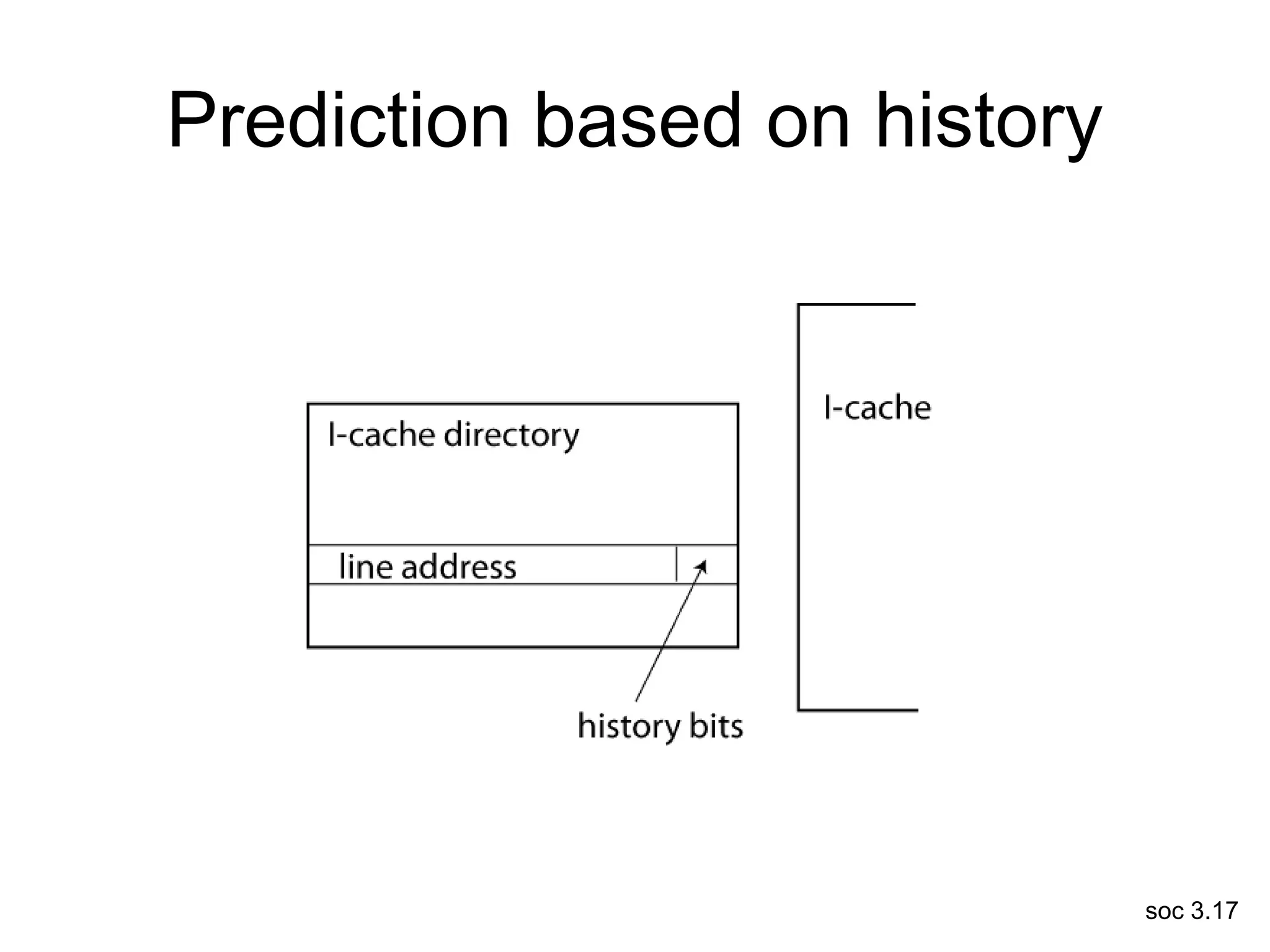
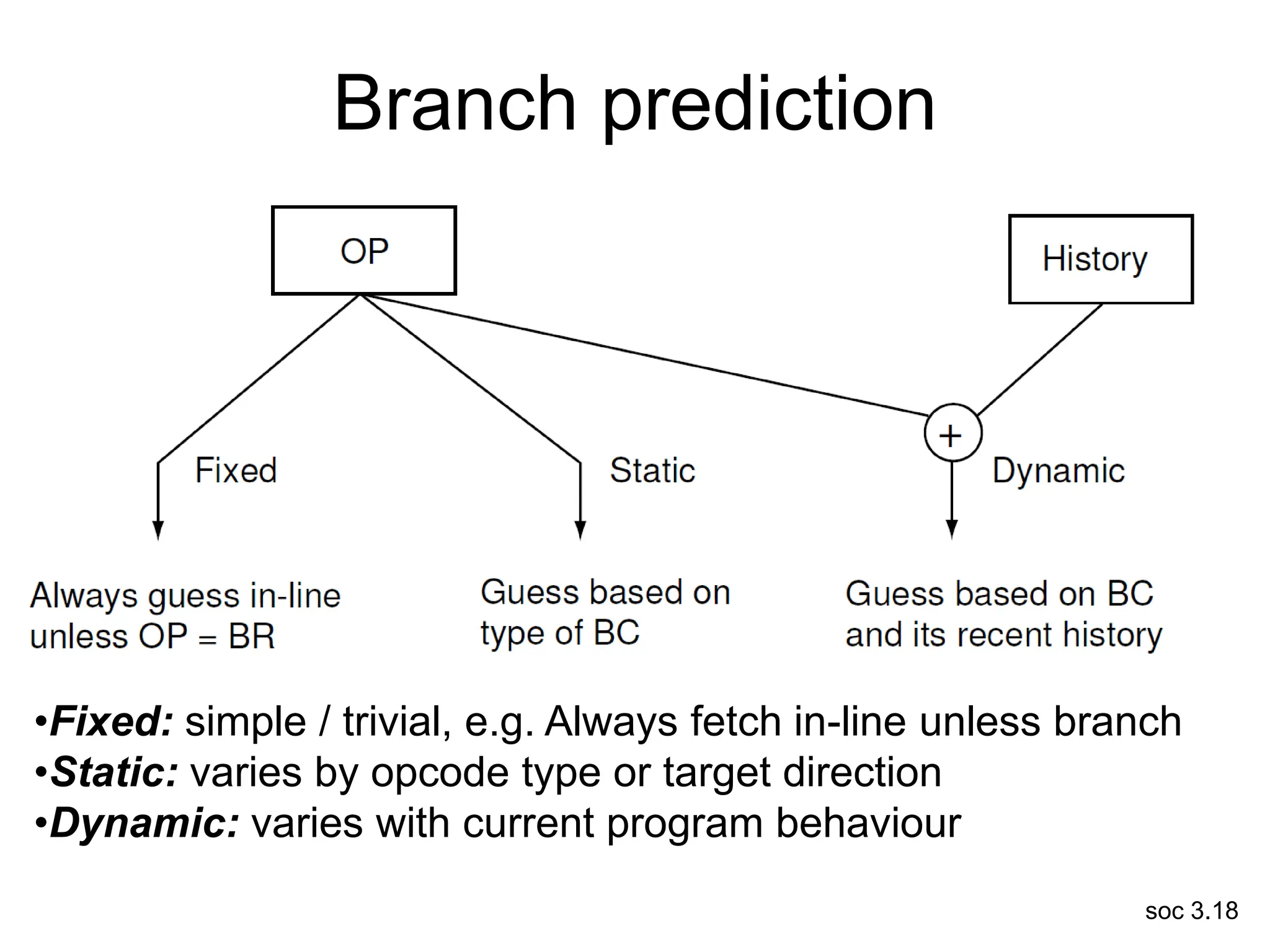
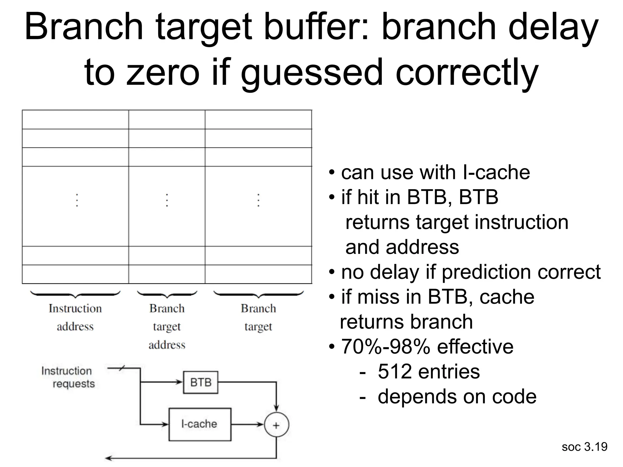
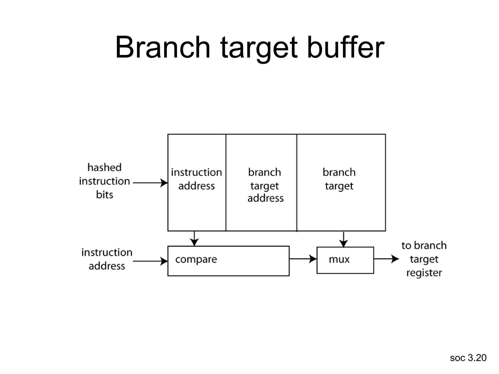
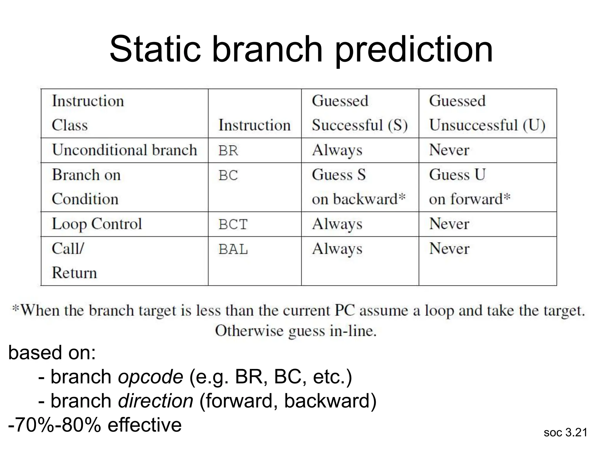
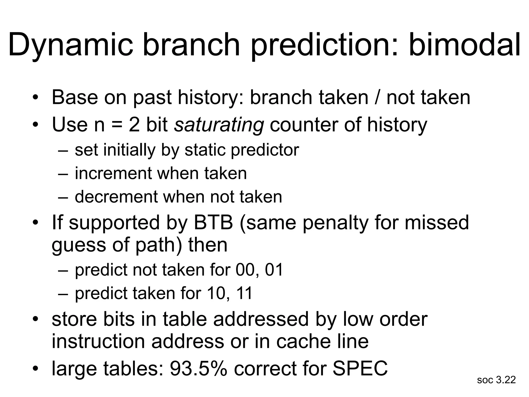
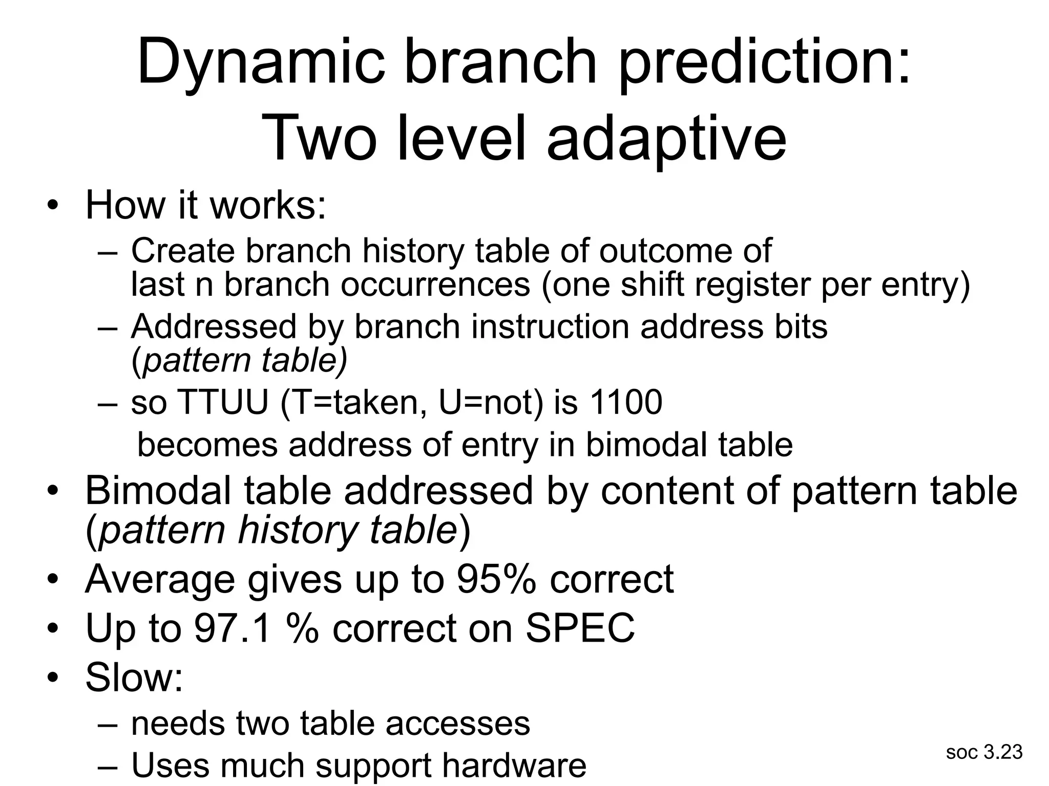
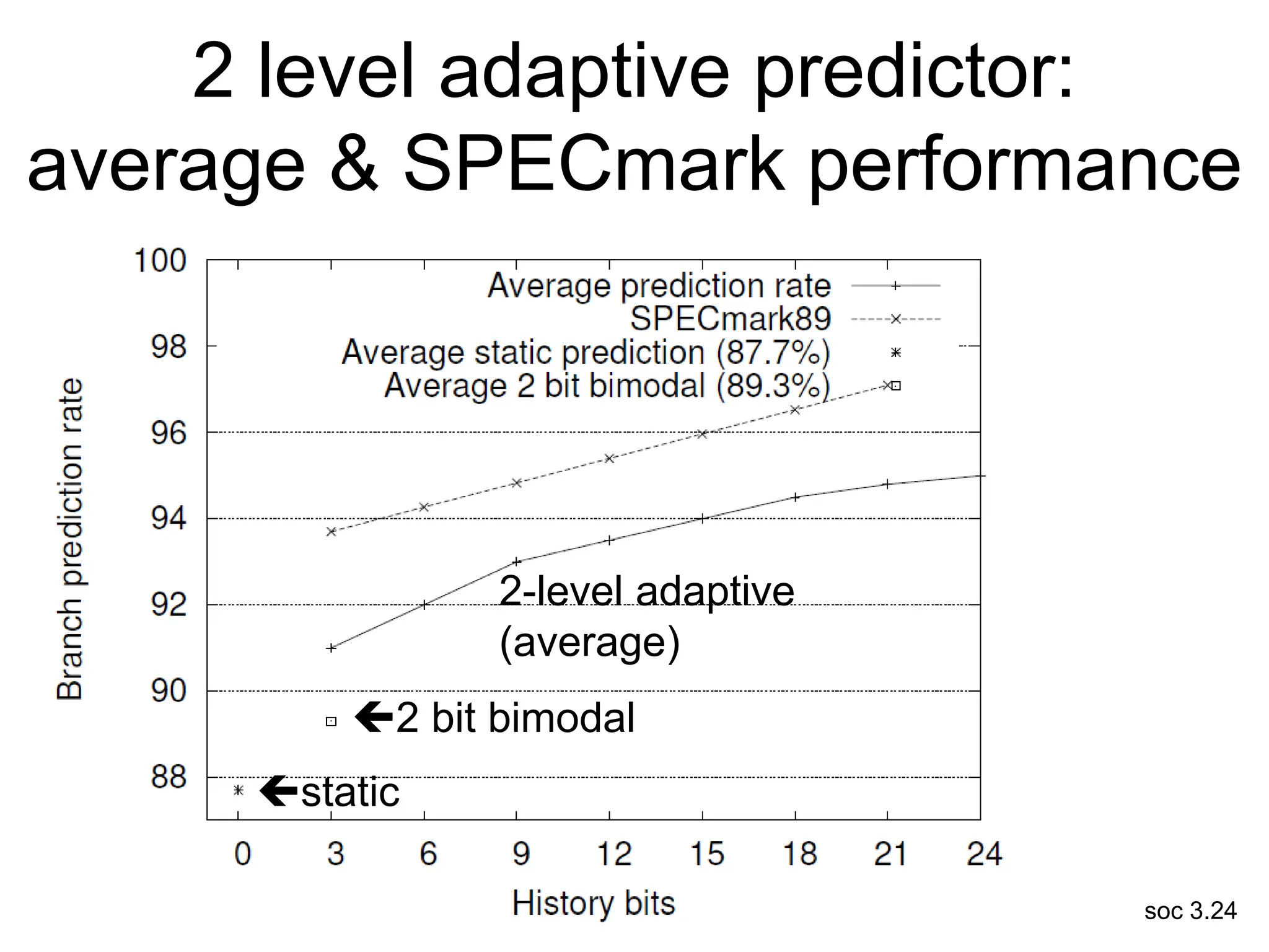
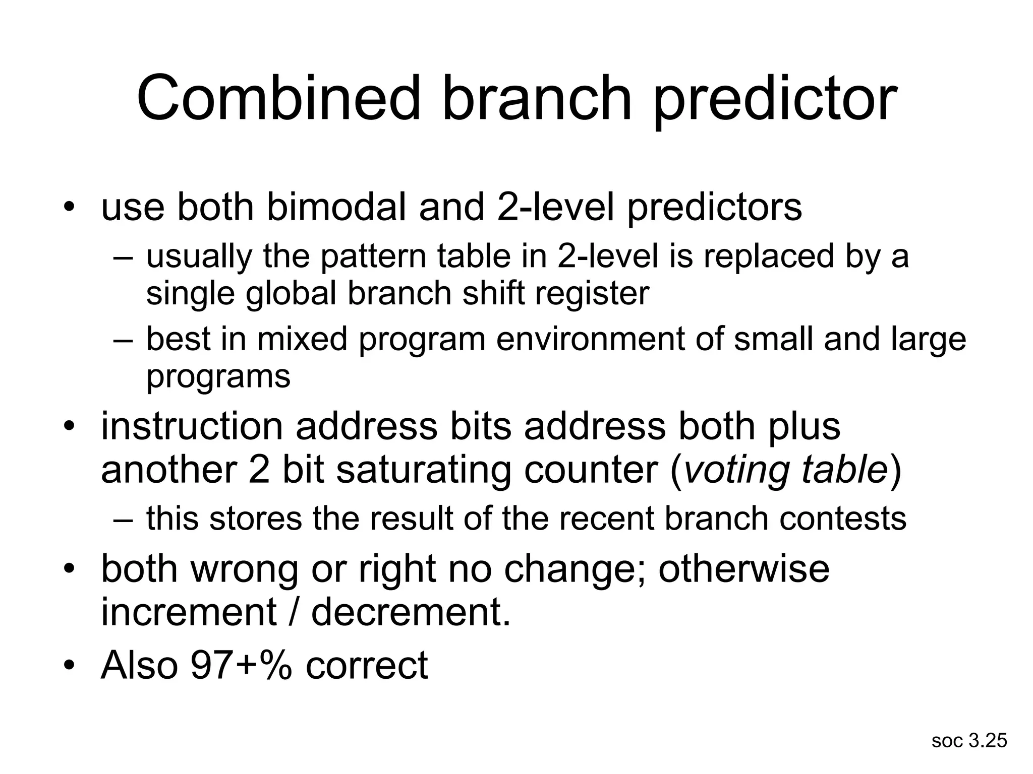
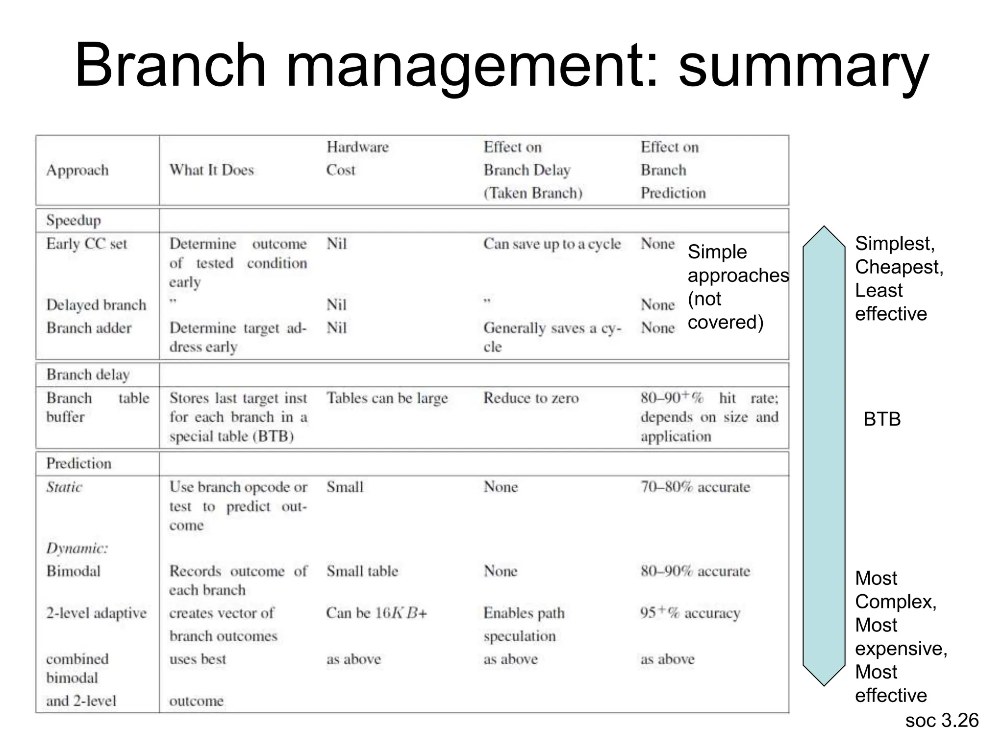
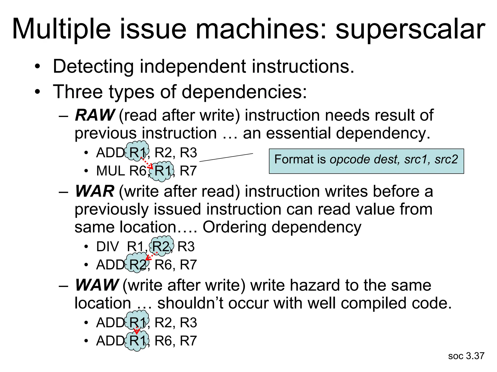
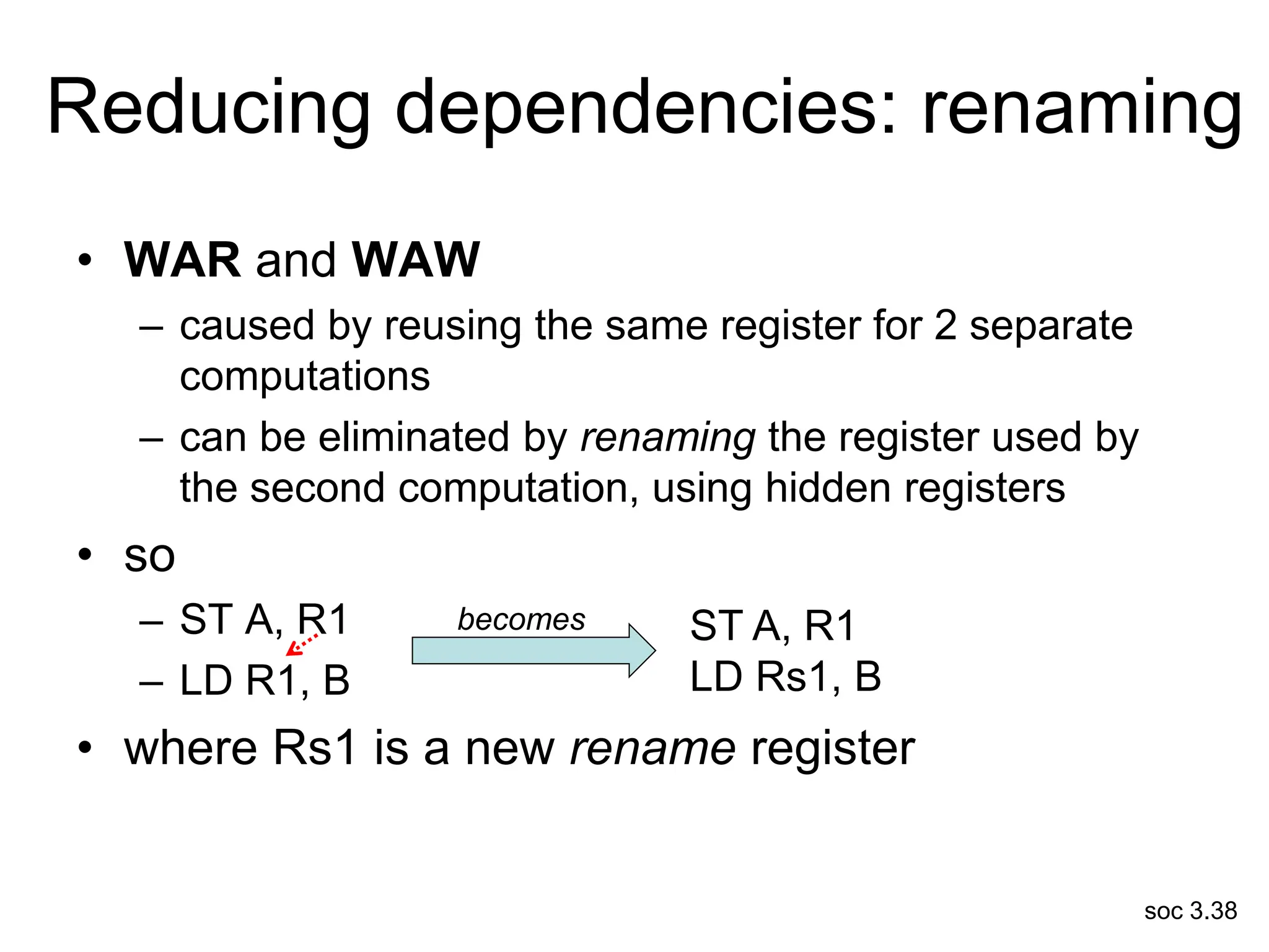
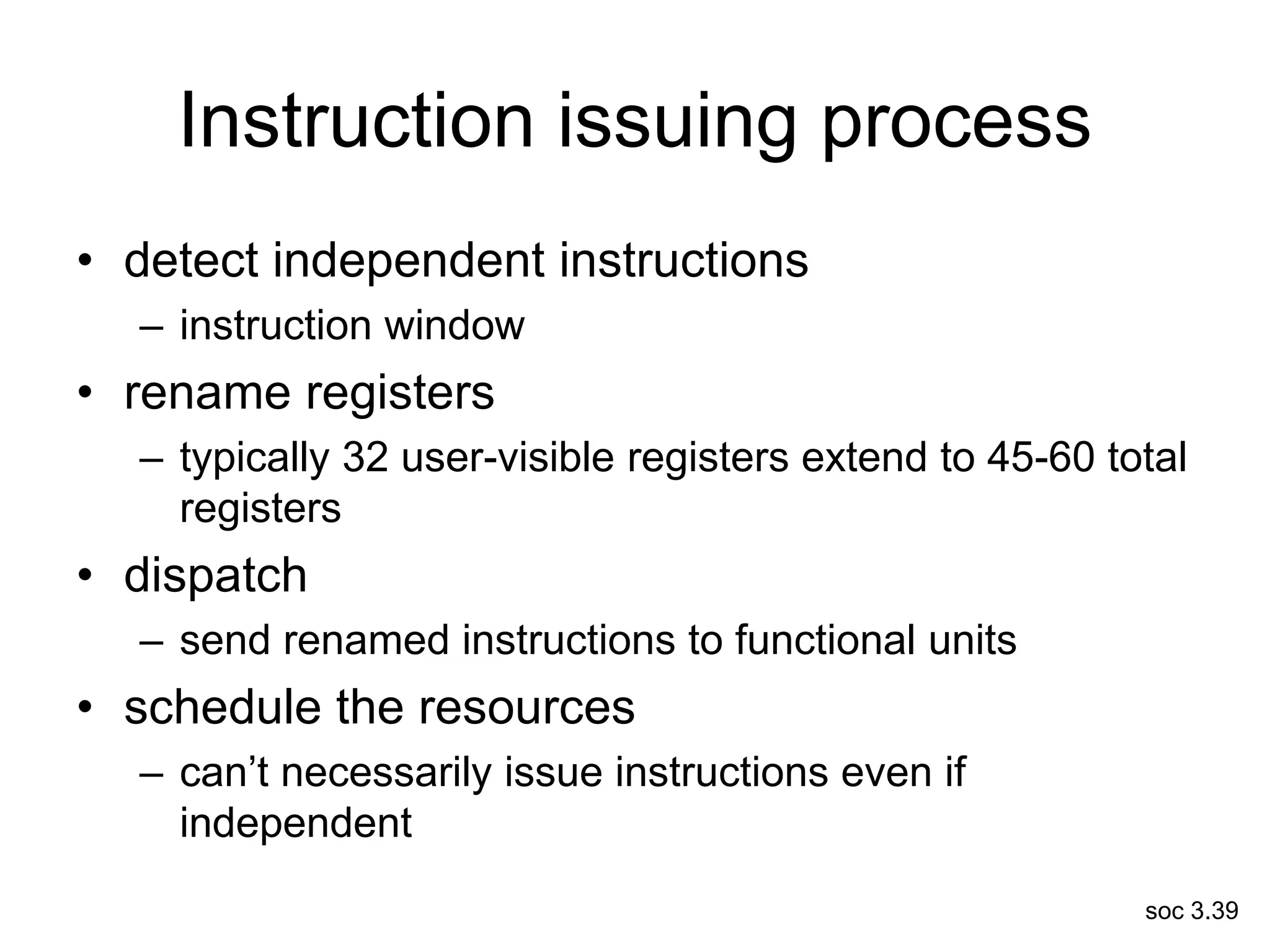
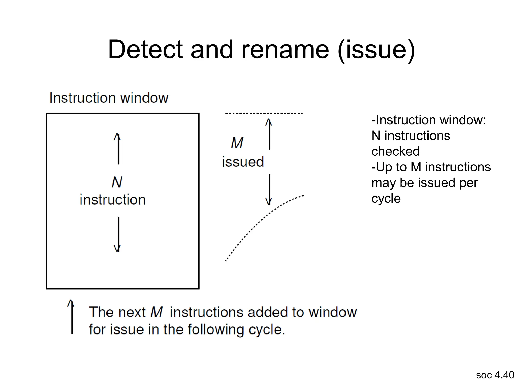
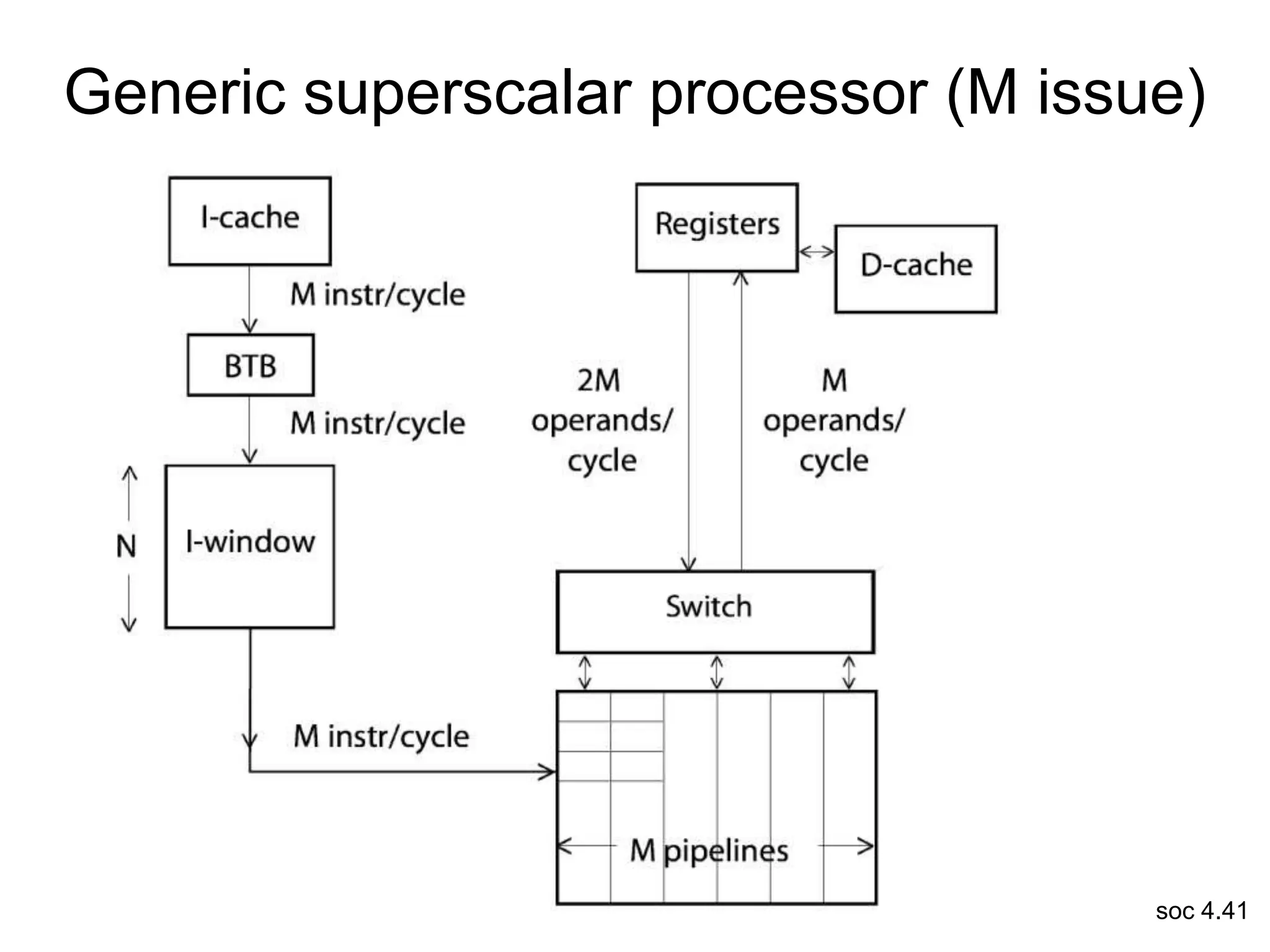
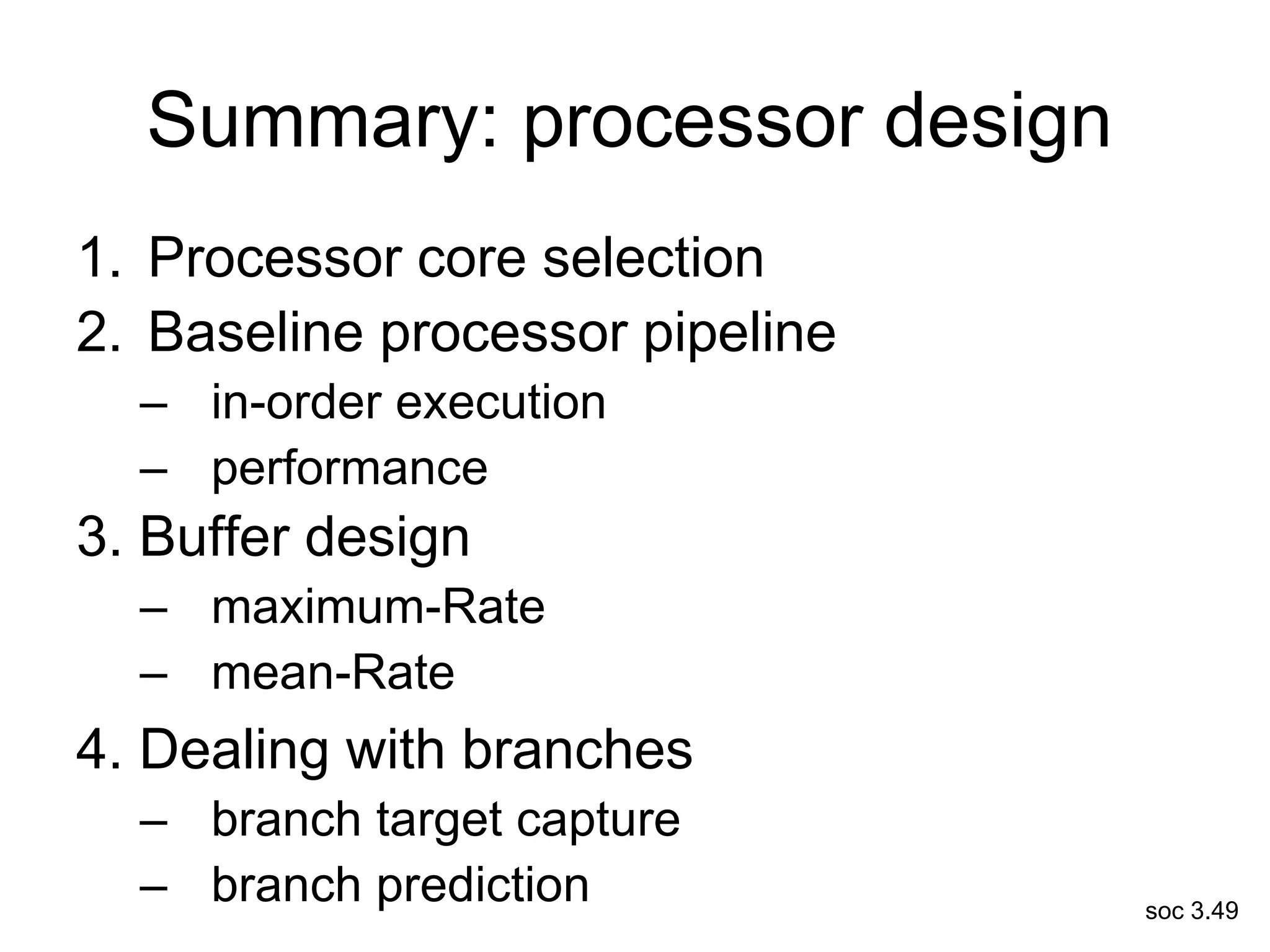
soc 3.1
Chapter 3
Processors
Computer System Design
System-on-Chip
by M. Flynn & W. Luk
Pub. Wiley 2011 (copyright 2011)
soc 3.2
Processor design: simple processor
1. Processor core selection
2. Baseline processor pipeline
– in-order execution
– performance
3. Buffer design
– maximum-Rate
– mean-Rate
4. Dealing with branches
– branch target capture
– branch prediction
soc 3.3
Processor design: robust processor
• vector processors
• VLIW processors
• superscalar processors
– our of order execution
– ensuring correct program execution
soc 3.4
1. Processor core selection
• constraints
– compute limited
• real-time limit
must address first
– other limitation
• balance design to
achieve constraints
• secondary targets
– software
– design effort
– fault tolerance
soc 3.5
Types of pipelined processors
soc 3.6
2. Baseline processor pipeline
• Optimum pipelining
– Depends on probability b of pipeline break
– Optimal number of stages Sopt =f(b)
• Need to minimize b to increase Sopt,
so must minimize effects of
– Branches
– Data dependencies
– Resource limitations
• Also must manage cache misses
soc 3.7
Simple pipelined processors
Interlocks: used to stall
subsequent instructions
soc 3.8
Interlocks
soc 3.9
In-order processor performance
• instruction execution time: linear sum of
decode + pipeline delays + memory delays
• processor performance breakdown
TTOTAL = TEX + TD + TM
TEX = Execution time
(1 + Run-on execution)
TD = Pipeline delays
(Resource,Data,Control)
TM = Memory delays
(TLB, Cache Miss)
soc 3.10
3. Buffer design
• buffers minimize memory delays
– delays caused by variation in throughput between the
pipeline and memory
• two types of buffer design criteria
– maximum rate for units that have high request rates
• the buffer is sized to mask the service latency
• generally keep buffers full (often fixed data rate)
• e.g. instruction or video buffers
– mean rate buffers for units with a lower expected
request rate
• size buffer design: minimize probability of overflowing
• e.g. store buffer
soc 3.11
Maximum-rate buffer design
• buffer is sized to avoid runout
– processor stalls, while buffer is empty awaiting service
• example: instruction buffer
– need buffer input rate > buffer output rate
– then size to cover latency at maximum demand
• buffer size (BF) should be:
– s: items processed (used or serviced) per cycle
– p: items fetched in an access
– First term: allow processing during current cycle
soc 3.12
Maximum-rate buffer: example
assumptions:
- decode consumes max 1 inst/clock
- Icache supplies 2 inst/clock bandwidth at 6 clocks latency
Branch Target Fetch
soc 3.13
Mean-rate buffer design
• use inequalities from probability theory to determine
buffer size
– Little’s theorem: Mean request size = Mean request rate (requests
/ cycle) * Mean time to service request
– for infinite buffer, assume:
distribution of buffer occupancy = q, mean occupancy = Q,
with standard deviation = 
• use Markov’s inequality for buffer of size BF
Prob. of overflow = p(q ≥ BF) ≤ Q/BF
• use Chebyshev’s inequality for buffer of size BF
Prob. of overflow = p(q ≥ BF) ≤ 2/(BF-Q)2
– given probability of overflow (p), conservatively select BF
BF = min(Q/p, Q + /√p)
– pick correct BF that causes overflow/stall
soc 3.14
Mean-rate buffer: example
Data
Cache
Store
Buffer
Memory
References
from
Pipeline
Reads
Writes
Assumptions:
• when store buffer is full, writes have priority
• write request rate = 0.15 inst/cycle
• store latency to data cache = 2 clocks
- so Q = 0.15 * 2 = 0.3 (Little’s theorem)
• given σ2 = 0.3
• if we use a 2 entry write buffer, BF=2
• P = min(Q/BF, σ2 / (BF-Q)2) = 0.10
soc 3.15
4. Dealing with branches
• need to eliminate branch delay
– branch target capture:
• branch table buffer (BTB)
• need to predict outcome
– branch prediction:
• static prediction
• bimodal
• 2 level adaptive
• combined
simplest, least accurate
most expensive,
most accurate
soc 3.16
Branch problem
- if 20% of instructions are BC (conditional branch),
may add delay of .2 x 5 cpi to each instruction
soc 3.17
Prediction based on history
soc 3.18
Branch prediction
•Fixed: simple / trivial, e.g. Always fetch in-line unless branch
•Static: varies by opcode type or target direction
•Dynamic: varies with current program behaviour
soc 3.19
Branch target buffer: branch delay
to zero if guessed correctly
• can use with I-cache
• if hit in BTB, BTB
returns target instruction
and address
• no delay if prediction correct
• if miss in BTB, cache
returns branch
• 70%-98% effective
- 512 entries
- depends on code
soc 3.20
Branch target buffer
soc 3.21
Static branch prediction
based on:
- branch opcode (e.g. BR, BC, etc.)
- branch direction (forward, backward)
-70%-80% effective
See **
soc 3.22
Dynamic branch prediction: bimodal
• Base on past history: branch taken / not taken
• Use n = 2 bit saturating counter of history
– set initially by static predictor
– increment when taken
– decrement when not taken
• If supported by BTB (same penalty for missed
guess of path) then
– predict not taken for 00, 01
– predict taken for 10, 11
• store bits in table addressed by low order
instruction address or in cache line
• large tables: 93.5% correct for SPEC
soc 3.23
Dynamic branch prediction:
Two level adaptive
• How it works:
– Create branch history table of outcome of
last n branch occurrences (one shift register per entry)
– Addressed by branch instruction address bits
(pattern table)
– so TTUU (T=taken, U=not) is 1100
becomes address of entry in bimodal table
• Bimodal table addressed by content of pattern table
(pattern history table)
• Average gives up to 95% correct
• Up to 97.1 % correct on SPEC
• Slow:
– needs two table accesses
– Uses much support hardware
soc 3.24
2 level adaptive predictor:
average & SPECmark performance
static
2 bit bimodal
2-level adaptive
(average)
soc 3.25
Combined branch predictor
• use both bimodal and 2-level predictors
– usually the pattern table in 2-level is replaced by a
single global branch shift register
– best in mixed program environment of small and large
programs
• instruction address bits address both plus
another 2 bit saturating counter (voting table)
– this stores the result of the recent branch contests
• both wrong or right no change; otherwise
increment / decrement.
• Also 97+% correct
soc 3.26
Branch management: summary
Simplest,
Cheapest,
Least
effective
Most
Complex,
Most
expensive,
Most
effective
BTB
Simple
approaches
(not
covered)
soc 3.27
More robust processors
• vector processors
• VLIW (very long instruction word) processors
• superscalar
soc 3.28
Vector stride corresponds to
access pattern
soc 3.29
Vector registers:
essential to a vector processor
soc 3.30
Vector instruction execution
depends on VR read ports
soc 3.31
Vector instruction execution with
dependency
soc 3.32
Vector instruction chaining
soc 3.33
Chaining path
soc 3.34
Generic vector processor
soc 3.35
Multiple issue machines: VLIW
• VLIW: typically over 200 bit instruction
word
• for VLIW most of the work is done by
compiler
– trace scheduling
soc 3.36
Generic VLIW processor
soc 3.37
• Detecting independent instructions.
• Three types of dependencies:
– RAW (read after write) instruction needs result of
previous instruction … an essential dependency.
• ADD R1, R2, R3
• MUL R6, R1, R7
– WAR (write after read) instruction writes before a
previously issued instruction can read value from
same location…. Ordering dependency
• DIV R1, R2, R3
• ADD R2, R6, R7
– WAW (write after write) write hazard to the same
location … shouldn’t occur with well compiled code.
• ADD R1, R2, R3
• ADD R1, R6, R7
Multiple issue machines: superscalar
Format is opcode dest, src1, src2
soc 3.38
Reducing dependencies: renaming
• WAR and WAW
– caused by reusing the same register for 2 separate
computations
– can be eliminated by renaming the register used by
the second computation, using hidden registers
• so
– ST A, R1
– LD R1, B
• where Rs1 is a new rename register
ST A, R1
LD Rs1, B
becomes
soc 3.39
Instruction issuing process
• detect independent instructions
– instruction window
• rename registers
– typically 32 user-visible registers extend to 45-60 total
registers
• dispatch
– send renamed instructions to functional units
• schedule the resources
– can’t necessarily issue instructions even if
independent
soc 4.40
Detect and rename (issue)
-Instruction window:
N instructions
checked
-Up to M instructions
may be issued per
cycle
soc 4.41
Generic superscalar processor (M issue)
soc 3.42
Dataflow management:
issue and rename
• Tomosulo’s algorithm
– issue instructions to functional units (reservation
stations) with available operand values
– unavailable source operands given name (tag) of
reservation station whose result is the operand
• continue issuing
– until unit reservation stations are full
– un-issued instructions: pending and held in buffer
– new instructions that depend on pending are also
pending
soc 4.43
Dataflow issue with reservation stations
Each reservation station:
-Registers to hold S1 and S2 values (if available), or
-Tags to indicate where values will come from
soc 3.44
Generic Superscalar
soc 3.45
Managing out of order execution
Simple register file
organization
Centralised reorder
buffer
soc 3.46
Managing out of order execution
Distributed reorder
buffer
soc 3.47
ARM processor (ARM 1020)
(in-order)
- simple, in-order
6-8 stage pipeline
- widely used in
SOCs
soc 3.48
Freescale E600 data paths
- used in complex SOCs
- out-of-order
- branch history
- vector instructions
- multiple caches
soc 3.49
Summary: processor design
1. Processor core selection
2. Baseline processor pipeline
– in-order execution
– performance
3. Buffer design
– maximum-Rate
– mean-Rate
4. Dealing with branches
– branch target capture
– branch prediction

SOC-CH3.pptSOC ProcessorsSOC Processors Used in SOC Used in SOC

  • 1.
    soc 3.1 Chapter 3 Processors ComputerSystem Design System-on-Chip by M. Flynn & W. Luk Pub. Wiley 2011 (copyright 2011)
  • 2.
    soc 3.2 Processor design:simple processor 1. Processor core selection 2. Baseline processor pipeline – in-order execution – performance 3. Buffer design – maximum-Rate – mean-Rate 4. Dealing with branches – branch target capture – branch prediction
  • 3.
    soc 3.3 Processor design:robust processor • vector processors • VLIW processors • superscalar processors – our of order execution – ensuring correct program execution
  • 4.
    soc 3.4 1. Processorcore selection • constraints – compute limited • real-time limit must address first – other limitation • balance design to achieve constraints • secondary targets – software – design effort – fault tolerance
  • 5.
    soc 3.5 Types ofpipelined processors
  • 6.
    soc 3.6 2. Baselineprocessor pipeline • Optimum pipelining – Depends on probability b of pipeline break – Optimal number of stages Sopt =f(b) • Need to minimize b to increase Sopt, so must minimize effects of – Branches – Data dependencies – Resource limitations • Also must manage cache misses
  • 7.
    soc 3.7 Simple pipelinedprocessors Interlocks: used to stall subsequent instructions
  • 8.
  • 9.
    soc 3.9 In-order processorperformance • instruction execution time: linear sum of decode + pipeline delays + memory delays • processor performance breakdown TTOTAL = TEX + TD + TM TEX = Execution time (1 + Run-on execution) TD = Pipeline delays (Resource,Data,Control) TM = Memory delays (TLB, Cache Miss)
  • 10.
    soc 3.10 3. Bufferdesign • buffers minimize memory delays – delays caused by variation in throughput between the pipeline and memory • two types of buffer design criteria – maximum rate for units that have high request rates • the buffer is sized to mask the service latency • generally keep buffers full (often fixed data rate) • e.g. instruction or video buffers – mean rate buffers for units with a lower expected request rate • size buffer design: minimize probability of overflowing • e.g. store buffer
  • 11.
    soc 3.11 Maximum-rate bufferdesign • buffer is sized to avoid runout – processor stalls, while buffer is empty awaiting service • example: instruction buffer – need buffer input rate > buffer output rate – then size to cover latency at maximum demand • buffer size (BF) should be: – s: items processed (used or serviced) per cycle – p: items fetched in an access – First term: allow processing during current cycle
  • 12.
    soc 3.12 Maximum-rate buffer:example assumptions: - decode consumes max 1 inst/clock - Icache supplies 2 inst/clock bandwidth at 6 clocks latency Branch Target Fetch
  • 13.
    soc 3.13 Mean-rate bufferdesign • use inequalities from probability theory to determine buffer size – Little’s theorem: Mean request size = Mean request rate (requests / cycle) * Mean time to service request – for infinite buffer, assume: distribution of buffer occupancy = q, mean occupancy = Q, with standard deviation =  • use Markov’s inequality for buffer of size BF Prob. of overflow = p(q ≥ BF) ≤ Q/BF • use Chebyshev’s inequality for buffer of size BF Prob. of overflow = p(q ≥ BF) ≤ 2/(BF-Q)2 – given probability of overflow (p), conservatively select BF BF = min(Q/p, Q + /√p) – pick correct BF that causes overflow/stall
  • 14.
    soc 3.14 Mean-rate buffer:example Data Cache Store Buffer Memory References from Pipeline Reads Writes Assumptions: • when store buffer is full, writes have priority • write request rate = 0.15 inst/cycle • store latency to data cache = 2 clocks - so Q = 0.15 * 2 = 0.3 (Little’s theorem) • given σ2 = 0.3 • if we use a 2 entry write buffer, BF=2 • P = min(Q/BF, σ2 / (BF-Q)2) = 0.10
  • 15.
    soc 3.15 4. Dealingwith branches • need to eliminate branch delay – branch target capture: • branch table buffer (BTB) • need to predict outcome – branch prediction: • static prediction • bimodal • 2 level adaptive • combined simplest, least accurate most expensive, most accurate
  • 16.
    soc 3.16 Branch problem -if 20% of instructions are BC (conditional branch), may add delay of .2 x 5 cpi to each instruction
  • 17.
  • 18.
    soc 3.18 Branch prediction •Fixed:simple / trivial, e.g. Always fetch in-line unless branch •Static: varies by opcode type or target direction •Dynamic: varies with current program behaviour
  • 19.
    soc 3.19 Branch targetbuffer: branch delay to zero if guessed correctly • can use with I-cache • if hit in BTB, BTB returns target instruction and address • no delay if prediction correct • if miss in BTB, cache returns branch • 70%-98% effective - 512 entries - depends on code
  • 20.
  • 21.
    soc 3.21 Static branchprediction based on: - branch opcode (e.g. BR, BC, etc.) - branch direction (forward, backward) -70%-80% effective See **
  • 22.
    soc 3.22 Dynamic branchprediction: bimodal • Base on past history: branch taken / not taken • Use n = 2 bit saturating counter of history – set initially by static predictor – increment when taken – decrement when not taken • If supported by BTB (same penalty for missed guess of path) then – predict not taken for 00, 01 – predict taken for 10, 11 • store bits in table addressed by low order instruction address or in cache line • large tables: 93.5% correct for SPEC
  • 23.
    soc 3.23 Dynamic branchprediction: Two level adaptive • How it works: – Create branch history table of outcome of last n branch occurrences (one shift register per entry) – Addressed by branch instruction address bits (pattern table) – so TTUU (T=taken, U=not) is 1100 becomes address of entry in bimodal table • Bimodal table addressed by content of pattern table (pattern history table) • Average gives up to 95% correct • Up to 97.1 % correct on SPEC • Slow: – needs two table accesses – Uses much support hardware
  • 24.
    soc 3.24 2 leveladaptive predictor: average & SPECmark performance static 2 bit bimodal 2-level adaptive (average)
  • 25.
    soc 3.25 Combined branchpredictor • use both bimodal and 2-level predictors – usually the pattern table in 2-level is replaced by a single global branch shift register – best in mixed program environment of small and large programs • instruction address bits address both plus another 2 bit saturating counter (voting table) – this stores the result of the recent branch contests • both wrong or right no change; otherwise increment / decrement. • Also 97+% correct
  • 26.
    soc 3.26 Branch management:summary Simplest, Cheapest, Least effective Most Complex, Most expensive, Most effective BTB Simple approaches (not covered)
  • 27.
    soc 3.27 More robustprocessors • vector processors • VLIW (very long instruction word) processors • superscalar
  • 28.
    soc 3.28 Vector stridecorresponds to access pattern
  • 29.
  • 30.
    soc 3.30 Vector instructionexecution depends on VR read ports
  • 31.
    soc 3.31 Vector instructionexecution with dependency
  • 32.
  • 33.
  • 34.
  • 35.
    soc 3.35 Multiple issuemachines: VLIW • VLIW: typically over 200 bit instruction word • for VLIW most of the work is done by compiler – trace scheduling
  • 36.
  • 37.
    soc 3.37 • Detectingindependent instructions. • Three types of dependencies: – RAW (read after write) instruction needs result of previous instruction … an essential dependency. • ADD R1, R2, R3 • MUL R6, R1, R7 – WAR (write after read) instruction writes before a previously issued instruction can read value from same location…. Ordering dependency • DIV R1, R2, R3 • ADD R2, R6, R7 – WAW (write after write) write hazard to the same location … shouldn’t occur with well compiled code. • ADD R1, R2, R3 • ADD R1, R6, R7 Multiple issue machines: superscalar Format is opcode dest, src1, src2
  • 38.
    soc 3.38 Reducing dependencies:renaming • WAR and WAW – caused by reusing the same register for 2 separate computations – can be eliminated by renaming the register used by the second computation, using hidden registers • so – ST A, R1 – LD R1, B • where Rs1 is a new rename register ST A, R1 LD Rs1, B becomes
  • 39.
    soc 3.39 Instruction issuingprocess • detect independent instructions – instruction window • rename registers – typically 32 user-visible registers extend to 45-60 total registers • dispatch – send renamed instructions to functional units • schedule the resources – can’t necessarily issue instructions even if independent
  • 40.
    soc 4.40 Detect andrename (issue) -Instruction window: N instructions checked -Up to M instructions may be issued per cycle
  • 41.
    soc 4.41 Generic superscalarprocessor (M issue)
  • 42.
    soc 3.42 Dataflow management: issueand rename • Tomosulo’s algorithm – issue instructions to functional units (reservation stations) with available operand values – unavailable source operands given name (tag) of reservation station whose result is the operand • continue issuing – until unit reservation stations are full – un-issued instructions: pending and held in buffer – new instructions that depend on pending are also pending
  • 43.
    soc 4.43 Dataflow issuewith reservation stations Each reservation station: -Registers to hold S1 and S2 values (if available), or -Tags to indicate where values will come from
  • 44.
  • 45.
    soc 3.45 Managing outof order execution Simple register file organization Centralised reorder buffer
  • 46.
    soc 3.46 Managing outof order execution Distributed reorder buffer
  • 47.
    soc 3.47 ARM processor(ARM 1020) (in-order) - simple, in-order 6-8 stage pipeline - widely used in SOCs
  • 48.
    soc 3.48 Freescale E600data paths - used in complex SOCs - out-of-order - branch history - vector instructions - multiple caches
  • 49.
    soc 3.49 Summary: processordesign 1. Processor core selection 2. Baseline processor pipeline – in-order execution – performance 3. Buffer design – maximum-Rate – mean-Rate 4. Dealing with branches – branch target capture – branch prediction