This document provides an overview of near-dissociation expansion (NDE) theory for quantizing energy levels of diatomic molecules near dissociation. Section 1 introduces the topic and outlines subsequent sections. Section 2 discusses the historical motivation of using the Birge-Sponer method to determine dissociation energies from spectroscopic data before NDE theory. Section 3 outlines the assumptions of NDE theory, including the Wentzel-Kramers-Brillouin approximation and representing the long-range potential as a dispersion expansion involving inverse powers of the internuclear separation.

1. Quantization of energy levels of a diatomic molecule near
dissociation
Stéphane Valladier
22nd
December, 2009 (v2.6)
1 Introduction
Under the Born-Oppenheimer approximation, two atoms bound in a diatomic molecule with inter-
nuclear separation R interact through a potential V(R). For energy levels lying sufficiently deep
within the potential well, the Dunham theory provides a relationship between the vibrational quan-
tum number, v, and the corresponding value of the energies. Likewise, for energy levels lying
within 10% of the potential well depth below the dissociation limit, Near-Dissociation Expansion
(NDE) theory gives approximate values for the vibrational energies as a function of v.
In Sec. 2, I’ll present the historical background that motivated the development of NDE theory.
Section 3 discusses the conditions underlying the validity of NDE theory. Section 4 summarizes
the derivation of the key results from the pioneering work of LeRoy and Bernstein [19]. In Sec. 5,
NDE theory is applied to the ground electronic state of H2 to predict energy levels and to Cl2
to derive properties of the B 3
Π+
0u electronic state. Section 6 reviews some of the improvements
recently achieved in NDE theory. The connection of NDE theory to current research topics, and
current developments of NDE theory itself are the objects of Sec. 7.
2 Historical background
One of the main interests of chemistry is knowing how much energy is required to dissociate a
molecule. The dissociation energy, De, is the amount of energy required to go from the bottom
of the potential well to the corresponding asymptote. Thus De depends on the electronic state
of the molecule. Another dissociation energy D0 is defined as the energy required to go from
the lowest (v = 0) vibrational level to the asymptote of the potential. The quantity D0 can be
1

2. seen as the quantum analog to De. Indeed De would be the actual dissociation energy of the
molecule in a purely classical treatment. The quantum dissociation energy D0 can be measured
from spectroscopic data, while De pertains to a fit of vibrational energies to a potential well. Figure
1 illustrate the difference between De and D0. Usually, the v = 0 energy level lies close to the
potential minimum, thus De and D0 are similar.
V
Ν 0
DeD0
Internuclear separation
Potentialenergy
Figure 1: Definition of the classical and quantum dissociation energies De and
D0 for a potential with asymptotic value V∞. The v = 0 level has been risen up
in the well to clarify the picture, usually this level is much closer to the potential
minimum.
To determine the dissociation energy of an electronic state of a diatomic molecule, in 1926
Birge and Sponer [1] proposed plotting vibrational spacings, ∆Gv+1/2 = E(v + 1) − E(v), vs. vibra-
tional quantum numbers. If all vibrational energies are known, D0 ≈ v=vmax−1
v=0 ∆Gv+1/2 = Evmax
−E0.
However in the 20’s, measuring high lying energy levels was not technologically possible. Hence
the reason for using the Birge-Sponer method. Figure 2 shows a Birge-Sponer plot for I2 in the
B 3
Π+
0u electronic state.
Extrapolation of the data from the last observed vibrational energy spacing to ∆Gv+1/2 = 0
yields the intercept with the v-axis, which estimates the vibrational quantum number of the last
energy level supported by the potential. Adding the area under the solid line in Fig. 2 to the highest
2

3. Figure 2: Typical Birge-Sponer plot, reproduced from LeRoy [16]. The data for
this figure come from Tbl. 1 in [4], and correspond to the B 3Π+
0u electronic state
of I2. The dashed line with vH = 72 is the highest quantum number that can be
plotted. Adding the area delimited by the dashes, the solid line, and the v-axis to
the highest measured energy yields De.
energy observed [4] gives an approximate value of De = 12, 439 cm−1
.
Until the work of LeRoy and Bernstein [19], the extrapolation from the last observed vibra-
tional spacing was often linear, as the expression for the vibrational energies in a Morse [26]
potential suggests. The accuracy of the dissociation energy calculated thus depends on the agree-
ment between the Morse potential and the true potential. LeRoy and Bernstein [19] improved
on the Birge-Sponer method by developing NDE theory, deriving an approximate relationship be-
tween the vibrational energies supported by an electronic state of a diatomic molecule and the
corresponding vibrational quantum number.
3 Underlying assumptions
3.1 WKB approximation
For vibrational wave functions near dissociation, the wavelength and amplitude remain almost con-
stant above the potential well, contrarily to lower-lying vibrational levels. Thus vibrational levels
near dissociation behave mostly as if the potential was constant. The Wentzel, Kramers, Brillouin
3

4. (WKB)1
method approximates the solution to the one-dimensional time-independent Schrödinger
equation when the potential energy varies slowly compared to the local de Broglie wavelength,
λ = 2π [2µ(E − V)]−1/2
. Hence the WKB approximation, explained in Bohm [2] and briefly sum-
marized in this section, is a stepping stone for the derivation of NDE theory.
The condition for applicability of the WKB approximation is given in [2] as:
µ
∂
∂R
V 2µ (E − V) 3/2
, (1)
where µ is the reduced mass of the molecule, E the molecule’s energy, and V(R) the potential
energy. Under the WKB approximation, considerations on the continuity of the wave function at
the classical turning points yields the Bohr-Sommerfeld quantization condition:
v +
1
2
=
2µ
π
R+
v
R−
v
Ev − V(R) dR, (2)
where v is the integer vibrational quantum number, and R−
v and R+
v are respectively the left and
right classical turning points of the v-th vibrational energy level, Ev = V(R−
v ) = V(R+
v ). Equation 2
is the starting point for the derivation of NDE theory summarized in Sec. 4.
3.2 Dispersion expansion
For energy levels near dissociation, the internuclear separation of a diatomic molecule is close to
the outer classical turning point R+
v , since the probability density accumulates there. Near dissoci-
ation, R+
v is sufficiently large for the electromagnetic forces between the individual constituents of
the diatomic molecule to dominate other interactions, such as electron exchange. As the Dunham
theory [27] exploits the simple harmonic oscillator approximation for a diatomic molecule near
equilibrium, likewise NDE theory exploits the analytic description of long-range forces dominant
near dissociation in a diatomic molecule.
For values of R large enough that the electron clouds of the individual atoms overlap negligibly,
1
Sometimes the name Jeffreys is added, giving JWKB.
4

5. the potential can be expressed as a sum of inverse powers of R [9, 21]:
V(R) ≈
R Re
V∞ −
k≥1
Ck
Rk
, (3)
where V∞ is the asymptotic value of the potential and Re is the internuclear separation at equilib-
rium. (If V(Re) = 0, then V∞ = De.) The powers k are positive integers, with values determined
by the nature of the interactions between the atoms involved in the molecule. The dispersion
coefficients Ck can be determined theoretically [5, 7, 22, 23, 25, 28] or experimentally [17, 24].
Each value of k in Eq. (3) represents a different physical interaction. A detailed description
of the meaning of each term is given in [16] and summarized here. The k = 1 term represents
the Coulomb potential between the atoms when they are charged. k = 2 corresponds classically
to a permanent dipole moment interacting with an ion. The k = 3 term models the interaction
between an ion and a permanent quadrupole moment, as weel as the resonant dipole-dipole inter-
action between the atoms. Homonuclear dimers dissociating to two different atomic states always
experience the latter interaction. The k = 4 term represents to first order the interaction of an ion
with an octupole, and a dipole and a quadrupole. To second order, the k = 4 term represents an ion
creating a charge-induced dipole on a neutral atom. For electronic states where neither atom disso-
ciates into an S state, the k = 5 term arises from the first order quadrupole-quadrupole interaction.
To second order, the k = 5 term models the interaction of a charged atom with induced dipole and
quadrupole, and the interaction of permanent monopole and dipole with an induced dipole. Certain
symmetries can make the C5 coefficient identically zero. All of the k values from 1 to 5 do not
necessarily occur for all molecules. Terms with k ≥ 6 are always present in Eq. (3) and represent
the van der Waals forces between the atoms. Other long-range terms like retardation effects can be
present in Eq. (3).
LeRoy [16, 17] estimates that the electron clouds of the atoms negligibly overlap for R greater
than
RLeR = 2 r
n | r2
| n 1/2
A + r
n | r2
| n 1/2
B [LeRoy radius], (4)
5

6. where the integration is carried over the radial r coordinate only and n, , n , , are the usual
quantum numbers2
for the atomic orbitals. The spherical harmonics being normalized, integration
over the angular coordinates yields 1 and removes the need to specify m , the orbital angular
momentum projection quantum number. Thus for R RLeR, the long-range exchange interaction
can be neglected; and RLeR is more meaningful than Re as a lower limit of R for the validity of
Eq. (3).
The definition of RLeR does not allow for the possibility for atoms to be in non spherically-
symmetric states. Figure 3 shows the quantity r
n | r2
| n 1/2
in red dashes for two identical
atoms. The distance between the center of the two red dashed circles is equal to the LeRoy radius
RLeR. If 0 for one the atoms, The electron cloud probability density is distorted by the spherical
harmonic Ym
(θ, ϕ) (blue solid line in Fig. 3). Then the two electron clouds can become sufficiently
close for other interactions then the ones described by Eq. (3), like exchange, to occur.
Figure 3: An idea of the LeRoy radius. The red dashed circles represent
r n | r2 | n 1/2. The distance between the center of the two circles is the LeRoy
radius given in Eq. (4). If one of the atoms has 0, the electron cloud probability
density is distorted by the spherical harmonic as shown by the blue solid line, drawn
for ( , m ) = (3, 0).
Ji et al. [12] modified Eq. (4) to account for the symmetry of the atomic states, which define
the orientation of the atomic orbitals. This modified LeRoy radius is:
RLeRm = 2
√
3 n m | z2
| n m 1/2
A + n m | z2
| n m 1/2
B , (5)
2
The principal quantum number n and the orbital angular momentum quantum number .
6

7. where the z-axis is the internuclear axis of the diatomic molecule, and the integration is carried
over all three spherical coordinates r, θ, and ϕ. With RLeRm, the range of validity of Eq. (3) changes
with the symmetry of the electronic potential, while it remained the same with RLeR (see [12]).
Figure 4 illustrates the difference between RLeR and RLeRm for the A1
Σ+
electronic state of NaCs.
Figure 4: Difference between RLeR and RLeRm for the A1Σ+ electronic state of
NaCs. The molecule dissociates to Na(3s)+Cs(6p). The long-range expansion is
clearly a better approximation to the potential for R > RLeRm.
4 Near Dissociation Expansion theory
This section summarizes the derivation of the semi-classical expression for the near-dissociation
vibrational levels in an electronic state of a dimer. An energy level is near dissociation when it lies
within 10% of the potential well depth below the dissociation limit. The detailed derivation can be
found in [19].
Near dissociation, the spacing between two successive energy levels is assumed sufficiently
small to treat the vibrational quantum number v in Eq. (2) as a differentiable function of the energy.
7

8. Differentiating v with respect to the energy yields the density of states
dv
dEv
=
2µ
2π
R+
v
R−
v
1
√
Ev − V(R)
dR. (6)
For vibrational energies near dissociation, the denominator of the integrand in Eq. (6) is close
to zero near the classical turning points, but comparatively large in between. Thus the integrand
is large near the classical turning points compared to its value in between. Moreover due to the
anharmonicity of the potential, the region near R+
v contributes more to the integral in Eq. (6) than
the region near R−
v . Consequently the integral will remain almost unchanged if the potential V(R)
is replaced by an approximate function accurate near R+
v (see Fig. 5).
Rv Rv
Potential
Approximate integrand
Integrand
Energy level
0
Internuclear separation
Figure 5: Plot of the integrand in Eq. (6). The potential is also given for context
and represents the X1Σ+ state of NaCs. The thick solid blue line is the v = 79
energy level and is located near dissociation as seen on the graph. The zero of
energy is at the asymptote of the potential. The area under the upper solid curve is
almost the same as the area under the dashed curve.
For example V(R) can be replaced by the leading term of Eq. (3):
V(R) = V∞ −
Cn
Rn
. (7)
8

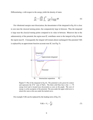
9. For near dissociation levels where R+
v → +∞, the integral in Eq. (6) can be calculated ([19] and
references therein), and an expression for the vibrational spacing between the high-lying energy
levels follows:
dEv
dv
=
2π
µ
Γ(1 + 1
n
)
Γ(1
2
+ 1
n
)
n
C1/n
n
(V∞ − Ev)
n+2
2n =
2n
n − 2
Hn(V∞ − Ev)
n+2
2n , (8)
with
Hn = (n − 2)
π
2µ
Γ(1 + 1
n
)
Γ(1
2
+ 1
n
)
C−1/n
n ,
where Γ(x) is the Euler Γ function. Integration of Eq. (8) with respect to v yields
V∞ − Ev = (Hn(vD − v))
2n
n−2 , (9)
where vD is a constant of integration interpreted as the (usually non-integer) vibrational quantum
number for a (non-existent) level with zero binding energy. The integer3
vD thus corresponds to
the quantum number of the last vibrational level supported by the potential. Hence, vD and the
number Nv of bound states in the potential satisfy Nv = vD + 1. For high-lying energy levels, a
non-linear fit of a data set (v, Ev) to Eq. (9) estimates the four parameters n, vD, Cn, and V∞. The
power n indicates the physical interaction that dominates the observed data, and Cn measures the
strength of the interaction. While n and Cn describe properties of the long-range potential, vD and
V∞ describe properties of the entire potential: the number of bound states and the dissociation
energy respectively. Once the four parameters of Eq. (9) are known, Eq. (9) gives estimates for the
energies of unobserved bound levels. An example is given in Sec. 5.
3
By definition, x =floor(x) is the greatest integer less than or equal to x.
9

10. 5 Examples
5.1 Hydrogen H2
As a test case, I consider the Kolos and Wolniewicz [14] H2(X1
Σ+
g ) potential. The same authors
reported the vibrational energies of this potential in [15].
Predicting vibrational energies with Eq. (9) requires n, vD, De, and Cn. By giving the full
potential, Ref. [14] provides De. From the description in Sec. 3.2 of the terms in Eq. (3), the leading
power in the long-range expansion is n = 6. Mitroy and Bromley [25] determined theoretically
the most recent values for the dispersion coefficients of H2 in its ground electronic state to high
precision, in particular C6 = 6.4990267054058 Eh a6
0.
Equation (2) estimates vD:
vD = −
1
2
+
(2µ)1/2
π
+∞
RvD
V∞ − V(R) dR, (10)
where RvD
is inner classical turning point of the (non-existent) energy level with zero binding
energy. For the H2(X1
Σ+
g ) potential of [14] vD = 14.936, consistent with the Nv = 15 bound states
reported in [15] and agreeing with experiments referenced therein.
Tbl. 1 compares the predictions of NDE theory, NDE
v , to the last seven vibrational energies
KW68
v of [15]. The agreement is best for levels v = 13 and 14. As v decreases, the agreement
deteriorates, since NDE theory is valid only for levels lying close to dissociation.
5.2 Halogens
As seen in Sec. 5.1, NDE theory can predict energy levels from information about a molecular
potential. Conversely, NDE theory can be used to deduce information about a molecular potential
from measured spectra. LeRoy and Bernstein [20] applied the theory to determine the dissociation
energy of some halogen dimers, along with the total number of bound levels. Their method is
essentially graphical. It assumes that the leading power n in Eq. (3) is known and that the spacing
10

11. Table 1: Comparison between bound-level energies calculated with NDE theory
and eigenenergies reported in [15] for the X1Σ+
g state of H2. The agreement is best
for the highest levels.
v KW68
v (Eh) NDE
v (Eh)
NDE
v − KW68
v
KW68
v
(%)
14 0.17384 0.17401 0.1
13 0.17102 0.17033 -0.4
12 0.16624 0.16003 -3.7
11 0.15979 0.13967 -12.6
10 0.15187 0.10583 -30.3
9 0.14264 0.05509 -61.4
8 0.13219 -0.01599 -112.0
between the energy levels is sufficiently small to validate the approximation
dEv
dv
≈ ∆Gv =
1
2
(∆Gv−1/2 + ∆Gv+1/2) =
1
2
(Ev+1 − Ev−1). (11)
Equation 8 can then be rewritten as
(∆Gv)2n/(n+2)
= (V∞ − Ev)
2n
n − 2
Hn
2n/(n+2)
. (12)
A plot of (∆Gv)2n/(n+2)
vs. Ev should be linear with x-intercept equal to V∞ and a slope propor-
tional to C−1/n
n . An example is given in Fig. 6 for the B 3
Π+
0u electronic state of Cl2, for which the
leading power is n = 5.
With V∞ known, a plot of (V∞ − Ev)(n−2)/2n
vs. v should be linear with x-intercept equal to vD.
This plot requires an assignment of vibrational quantum numbers to the energy levels. With Cn
known, the vibrational assignment can be adjusted so all the data falls on the same line. Figure 7
shows such a plot. A close look at Fig. 7 also emphasizes the breakdown of NDE theory for energy
levels further from dissociation. As the binding energy (V∞ −Ev) increases, the data points in Fig. 7
11

12. Figure 6: Plot of (∆Gv)2n/(n+2) vs. Ev for the B 3Π+
0u electronic state of Cl2. The
higher the energy, the more the data points fall on the line. The x-intercept is
marked to show the value of V∞.
move away from the predicated line.
6 Improving NDE
The derivation of NDE theory relies on the first order WKB approximation leading to Eq. (2) and
on the evaluation of the integral in Eq. (6). Comparat [6] developed an improved NDE expression
for binding energies that is valid in a region where the next dispersion term Cm/Rm
(m > n) con-
tributes no more than 1% of the leading term Cn/Rn
. According to [6], improving the quantization
condition Eq. (2) is not necessary to improve Eq. (9). Instead, the improvement focuses on a better
determination of the integral in Eq. (6). The derivation relies on splitting the integration interval of
Eq. (6) into three regions and approximating the integrand in each region to get an improved ap-
proximation to the total integral. Integration of the resulting expression then yields the improved
12

13. Figure 7: Plot of (V∞ − Ev)(n−2)/2n vs. v for the B 3Π+
0u electronic state of Cl2.
As in Fig. 6, the higher the energy, the more the data points fall on the line. The
x-intercept is marked to show the value of vD.
NDE formula
vD − v = H−1
n (V∞ − Ev)
n−2
2n + γ(V∞ − Ev), (13)
where γ is a real coefficient depending on how the initial integral in Eq. (6) is split. Comparat [6]
circumvents the dependences of γ on the splitting procedure by treating γ as a parameter. Equation
(13) is inverted in [6] by considering the second term on the right-hand side as a perturbation,
yielding:
V∞ − Ev = (Hn(vD − v))
2n
n−2 1 −
2n
n − 2
γ (Hn(vD − v))
2n
n−2 −1
. (14)
NDE theory can also be improved by including the next leading dispersion term, Cm/Rm
, in
Eq. (6) which has been studied by LeRoy [18], Comparat [6], and Jelassi et al. [10]. LeRoy ob-
tained an expression for the vibrational spacing as a function of the binding energy, but4
his result
is invalid for n = 3, m = 6. Comparat applies his integral splitting technique to the work of [18]
and obtains an expression for vD − v of the form:
vD − v = an(V∞ − Ev)
n−2
2n + ˜γδ(V∞ − Ev) + Cmbnm fnm(V∞ − Ev)
2m−n−2
2n . (15)
4
See Tbl. II in [18].
13

14. For more details on Eq. (15), see [6]. Thanks to the integral splitting technique, Equation (15) is
valid for (n, m) = (3, 6).
For the ground electronic state of homonuclear molecules, the two leading terms in Eq. (3) have
n = 3 and m = 6. The atomic lifetime can be extracted from C3. When one atom is in its ground
state, and the other is in a P state [13],
τ =
3 c3
4C3ω3
. (16)
Despite the validity of Eq. (15) in the (n, m) = (3, 6) case, Jelassi et al. [10] refined the expression
for vD − v from [6] by distinguishing between weakly and very weakly bound energy levels. For
(n, m) = (3, 6) and very weakly bound energy levels, vD −v depends on (V∞ − Ev)1/6
, (V∞ − Ev), and
(V∞ − Ev)2
. For (n, m) = (3, 6) and weakly bound energy levels, an additional (V∞ − Ev)7/6
appears
due to the magnitude of the binding energy compared to the ratio (Cm
n /Cn
m)1/(m−n)
.
7 NDE in Ultracold Physics
NDE theory is a useful tool for experimentalists. Recently, Wang et al. [29] reported the use of
the improved NDE theory expression Eq. (13) to determine the resonant dipole-dipole dispersion
coefficient C3 for the 0−
g , 1g, and 0+
u states of Cs2 using ultracold photoassociation spectroscopy.
With the C3 obtained, atomic lifetimes can be determined.
Gribakin and Flambaum [8] derived an expression for the scattering length as a function of the
leading exponent n in Eq. (3), the corresponding dispersion coefficient Cn, and the semiclassical
phase at zero energy, Φ:
a = ¯a 1 − tan
π
n − 2
tan Φ −
π
2(n − 2)
. (17)
14

15. In Eq. (17), ¯a is the mean scattering length defined by:
¯a = cos
π
n − 2


2µCn
(n − 2)


2
n−2
Γ(n−3
n−2
)
Γ(n−1
n−2
)
, (18)
and Φ is:
Φ =
1 +∞
R0
V∞ − V(R) dR, (19)
where R0 is the internuclear separation such that the potential crosses its asymptote. It is striking
to notice that RvD
from Eq. (10) and R0 have the same definition. Therefore,
Φ = vD +
1
2
π. (20)
Thus, the use of NDE theory with a few high lying vibrational levels can yield the scattering length
of an electronic potential.
8 Conclusion
Given the vibrational quantum number, NDE theory approximates the energy of a high lying bound
level in an electronic potential of a dimer. This approximation can be used with spectroscopic data
to yield estimates for the dissociation energy, the total number of bound states it supports, and the
value of the leading dispersion coefficient.
Although developed in the early 70’s, NDE theory is still being improved and is relevant to
research being done today. Retardation effects occurring at very long range have yet to be included
for energy levels higher in the potential. An extension of NDE theory to include the third term
from the long range expansion Eq. (3) remains to be studied.
References
[1] R. T. Birge and H. Sponer. The heat of dissociation of non-polar molecules. Physical Review,
28(2):259–283, August 1926. URL http://link.aps.org/abstract/PR/v28/p259.
15

16. [2] David Bohm. Quantum Theory. Prentice-Hall, Inc., 1st edition, 1951.
[3] C. Boisseau, E. Audouard, and J. Vigué. Quantization of the highest levels in a molecular
potential. Europhysics Letters, 41(4):349–354, February 1998.
[4] Weldon G. Brown. Note on the heat of dissociation of iodine. Physical Review, 38(4):709–
711, August 1931. URL http://link.aps.org/abstract/PR/v38/p709.
[5] Béatrice Bussery, Yamina Achkar, and Monique Aubert-Fécon. Long-range molecular
states dissociating to the three or four lowest asymptotes for the ten heteronuclear diatomic
alkali molecules. Chemical Physics, 116:319–338, 1987.
[6] Daniel Comparat. Improved LeRoy-Bernstein near-dissociation expansion for-
mula, and prospect for photoassociation spectroscopy. The Journal of Chem-
ical Physics, 120(3):1318–1329, 2004. doi: 10.1063/1.1626539. URL
http://link.aip.org/link/?JCP/120/1318/1.
[7] A. Derevianko, J. F. Babb, and A. Dalgarno. High-precision calculations of van der Waals
coefficients for heteronuclear alkali-metal dimers. Physical Review A, 63:052704, 2001.
[8] G. F. Gribakin and V. V. Flambaum. Calculation of the scattering length in atomic collisions
using the semiclassical approximation. Physical Review A, 48(1):546–, July 1993. URL
http://link.aps.org/abstract/PRA/v48/p546.
[9] Joseph O. Hirschfelder, Charles F. Curtiss, and R. Byron Bird. Molecular Theory of Gases
and Liquids. Structure of Matter. John Wiley and Sons, Inc, New York, 1954.
[10] Haikel Jelassi, Bruno Viaris de Lesegno, and Laurence Pruvost. Reexami-
nation of the LeRoy-Bernstein formula for weakly bound molecules. Physi-
cal Review A, 77(6):062515, 2008. doi: 10.1103/PhysRevA.77.062515. URL
http://link.aps.org/abstract/PRA/v77/e062515.
[11] Haikel Jelassi, Bruno Viaris de Lesegno, Laurence Pruvost, Marin Pichler, and
William C. Stwalley. Spin effects in (6s1/2 + 6p1/2) 0+
u
133
Cs2 weakly bound
molecules analyzed by using the Lu-Fano method coupled to the improved LeRoy–
Bernstein formula. Physical Review A, 78(2):022503, August 2008. URL
http://link.aps.org/abstract/PRA/v78/e022503.
[12] Bing Ji, Chin-Chun Tsai, and William C. Stwalley. Proposed modification of the criterion
for the region of validity of the inverse-power expansion in diatomic long-range potentials.
Chemical Physics Letters, 236:242–246, 1995.
[13] Kevin M. Jones, Eite Tiesinga, Paul D. Lett, and Paul S. Julienne. Ultracold photoassociation
spectroscopy: long-range molecules and atomic scattering. Review of Modern Physics, 78:
483–535, May 2006. doi: 10.1103/RevModPhys.78.483.
[14] W. Kolos and L. Wolniewicz. Potential-energy curves for the X1
Σ+
g , b3
Σ+
u , and C1
Πu states
of the hydrogen molecule. The Journal of Chemical Physics, 43(7):2429–2441, 1965. doi:
10.1063/1.1697142. URL http://link.aip.org/link/?JCP/43/2429/1.
16

17. [15] W. Kolos and L. Wolniewicz. Improved theoretical ground-state energy of the hydrogen
molecule. The Journal of Chemical Physics, 49(1):404–410, 1968. doi: 10.1063/1.1669836.
URL http://link.aip.org/link/?JCP/49/404/1.
[16] Robert J. LeRoy. Molecular Spectroscopy, Specialist periodical reports, volume 1, chapter
3: Energy levels of a diatomic near dissociation, pages 113–176. 1973.
[17] Robert J. LeRoy. Long-range potential coefficients from RKR turning points: C6 and C8 for
B(3
Π+
0u)-State Cl2, Br2, and I2. Canadian Journal of Physics, pages 246–256, 1974.
[18] Robert J. LeRoy. Theory of deviations from the limiting near-dissociation behavior of
diatomic molecules. The Journal of Chemical Physics, 73(12):6003–6012, 1980. doi:
10.1063/1.440134. URL http://link.aip.org/link/?JCP/73/6003/1.
[19] Robert J. LeRoy and B. Bernstein. Dissociation energy and long range potential of diatomic
molecules from vibrational spacings of higher levels. Journal of Chemical Physics, 52(8):
3869–3879, 1970. URL http://link.aip.org/link/?JCP/52/3869/1.
[20] Robert J. LeRoy and B. Bernstein. Dissociation energies and long range potentials of di-
atomic molecules from vibrational spacings : the halogens. Journal of Molecular Spec-
troscopy, 37:109–130, 1971.
[21] H. Margenau. Van der Waals forces. Review of Modern Physics, 11(1):1–35, January 1939.
URL http://link.aps.org/abstract/RMP/v11/p1.
[22] Henry Margenau. Quadrupole contributions to London’s dispersion forces. The Jour-
nal of Chemical Physics, 6(12):896–899, 1938. doi: 10.1063/1.1750184. URL
http://link.aip.org/link/?JCP/6/896/1.
[23] M. Marinescu and H. R. Sadeghpour. Long range potentials for two-species
alkali-metal atoms. Physical Review A, 59(1):390–404, January 1999. URL
http://link.aps.org/abstract/PRA/v59/p390.
[24] W. I. McAlexander, E. R. I. Abraham, and R. G. Hulet. Radiative lifetime of
the 2p state of lithium. Physical Review A, 54(1):R5–R8, July 1996. URL
http://link.aps.org/abstract/PRA/v54/pR5.
[25] J. Mitroy and M. W. J. Bromley. Higher-order Cn dispersion coeffi-
cients for hydrogen. Physical Review A, 71(3):032709, 2005. URL
http://link.aps.org/abstract/PRA/v71/e032709.
[26] Philip M. Morse. Diatomic molecules according to the wave mechan-
ics. II. Vibrational levels. Physical Review, 34(1):57–64, July 1929. URL
http://link.aps.org/abstract/PR/v34/p57.
[27] J. F. Ogilvie. The vibrational and rotational spectrometry of diatomic molecules. Academic
Press, 1998.
17

18. [28] Sergey G. Porsev and Andrei Derevianko. Accurate relativistic many-body calcula-
tions of van der Waals coefficients C8 and C10 for alkali-metal dimers. The Jour-
nal of Chemical Physics, 119(2):844–850, 2003. doi: 10.1063/1.1578052. URL
http://link.aip.org/link/?JCP/119/844/1.
[29] L.R. Wang, J. Ma, C.Y. Li, J.M. Zhao, L.T. Xiao, and S.T. Jia. High sensitive photoassociation
spectroscopy based on modulated ultra-cold Cs atoms. Applied Physics B: Lasers and Optics,
89(1):53–57, October 2007. URL http://dx.doi.org/10.1007/s00340-007-2737-0.
18