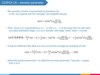
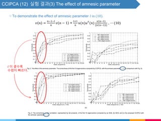
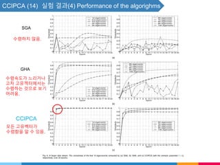
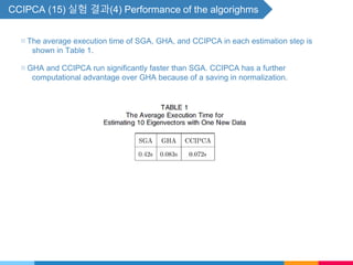
This document summarizes the Candid Covariance-Free Incremental Principal Component Analysis (CCIPCA) algorithm. CCIPCA incrementally estimates principal components from sequentially arriving sample vectors without storing a covariance matrix. It uses an iterative approach to estimate each eigenvector, subtracting the effect of prior eigenvectors from new samples. The algorithm includes an "amnesic parameter" l to weight more recent samples more heavily. Experimental results on face image data show CCIPCA converges faster and more accurately than other incremental PCA methods.

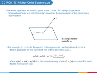
![CCIPCA (9) - 실험 준비
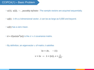
▧ We define sample-to-dimension ratio as
𝑛
𝑑
, where 𝑛 is the number of samples and
𝑑 is the dimension of the sample space.
▧ First presented here are our results on the FERET face data set [18]. The data set has 982
images. The size of each image is 88 x 64 pixels or 5,632 dimensions.
▧ The sample-to-dimension ratio as
982
5632
= 0.17
▧ We computed the eigenvectors using a batch PCA with QR method and used them as our
gound truth. The program for batch PCA was adapted from the C Recipes [9].
▧ Since the real mean of the image data is unknown. We incrementally estimated the sample
mean 𝑚(𝑛) by
𝑚 𝑛 =
𝑛−1
𝑛
𝑚 𝑛 − 1 +
1
𝑛
𝑥(𝑛)
where 𝑥(𝑛) is the 𝑛th sample image.
▧ The data entering the IPCA algorithms are the scatter vectors,
𝑢 𝑛 = 𝑥 𝑛 − 𝑚 𝑛 , 𝑛 = 1, 2, ⋯](https://image.slidesharecdn.com/seminar9-180126085316/85/Seminar9-10-320.jpg)
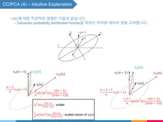
![CCIPCA (5) - Higher-Order Eigenvectors - 보충자료
▧ One way to compute the other higher order eigenvectors is following what SGA does.
SGA(Stochastic gradient ascent).
Start with a set of orthonormalized vectors, update them using the suggested iteration
step and recover the orthogonality using GSO.
SGA computes, Oja and Karhunen[9, 10],
𝑣𝑖 𝑛 = 𝑣𝑖 𝑛 − 1 + 𝛾𝑖 𝑢 𝑛 𝑢 𝑇
𝑛 𝑣𝑖 𝑛 − 1 ⋯ (6)
𝑣𝑖 𝑛 = 𝑜𝑟𝑡ℎ𝑜𝑛𝑜𝑟𝑚𝑎𝑙𝑖𝑧𝑒 𝑣𝑖 𝑛 w.r.t. 𝑣𝑗(𝑛), 𝑗 = 1, 2, ⋯ , 𝑖 − 1. ⋯ (7)
where 𝑣𝑖 𝑛 is the estimate of the 𝑖th dominant eigenvectors of the sample covariance
matrix.](https://image.slidesharecdn.com/seminar9-180126085316/85/Seminar9-18-320.jpg)