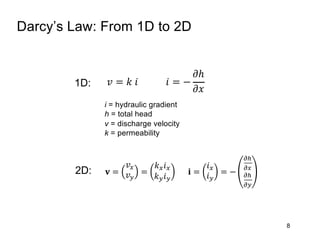
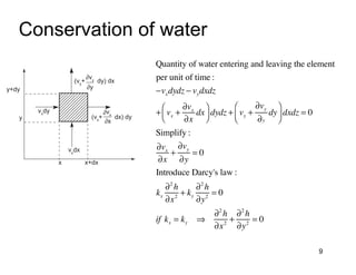
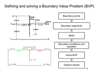
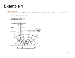
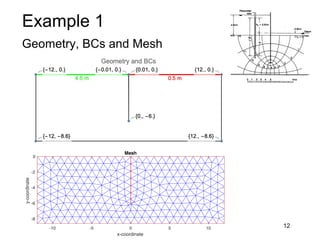
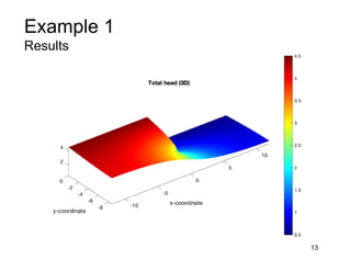
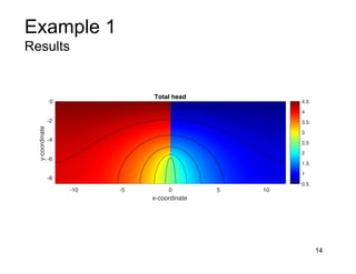
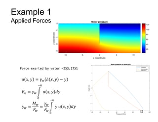
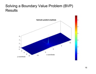
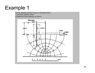
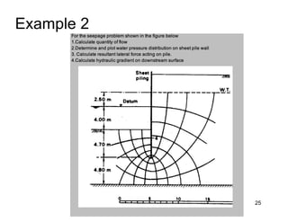
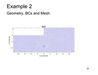
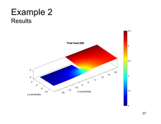
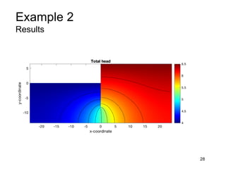
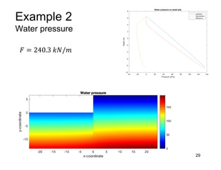
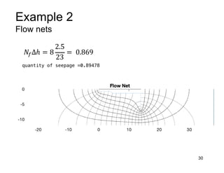
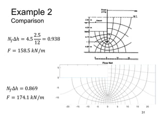
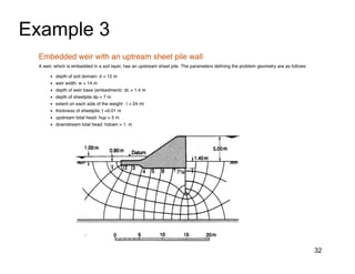
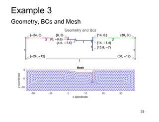
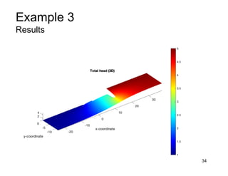
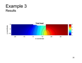
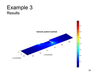
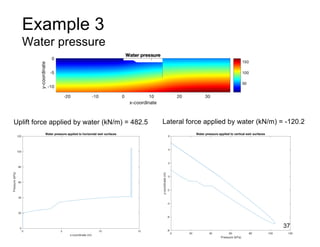
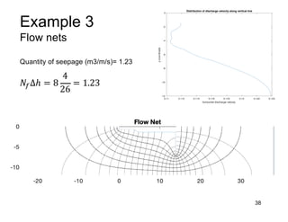
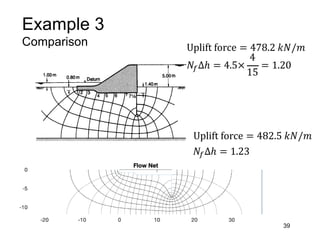
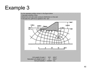
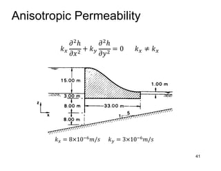
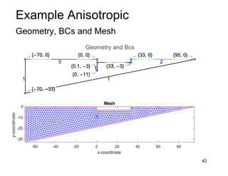
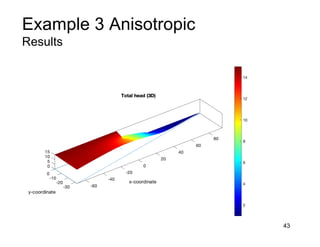
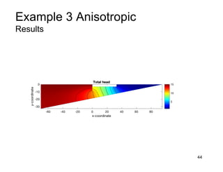
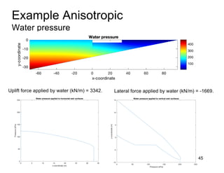
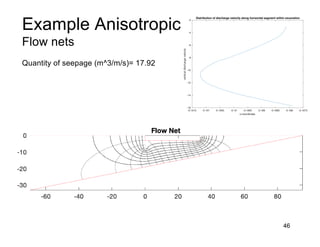
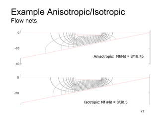
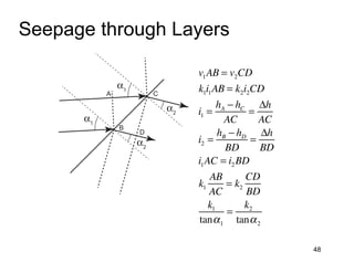
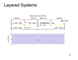
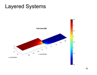
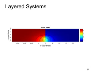
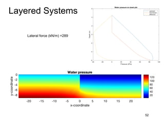
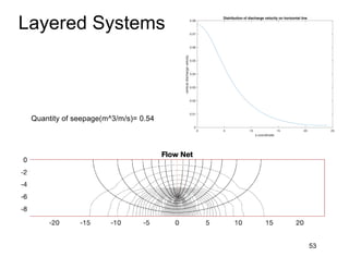
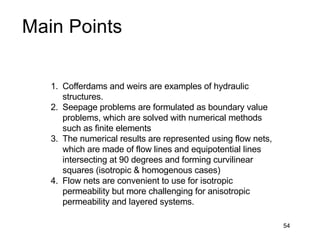
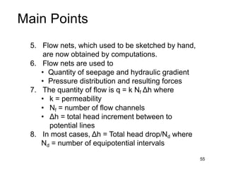
CE 470
Foundations and
Earth Retaining Systems
Seepage
Jean-Pierre Bardet
University of Miami
2
Learning Objectives
1. Identify examples of real seepage problems
2. Define the equation governing how water
seeps through soils
3. Formulate seepage as a boundary value
problem
4. Overview finite elements methods for solving
seepage boundary value problems
5. Apply computational results, i.e., flow nets, to
obtain engineering quantities:
• quantity of seepage
• pressure and forces, and
• hydraulic gradients
Sheet Pile Walls
Sheet Pile Walls
Sheet Pile Walls
Sheet Pile Walls
Weirs
Darcy’s Law: From 1D to 2D
8
𝐯 =
𝑣!
𝑣"
=
𝑘!𝑖!
𝑘"𝑖"
𝐢 =
𝑖!
𝑖"
= −
#$
#!
#$
#"
𝑣 = 𝑘 𝑖 𝑖 = −
𝜕ℎ
𝜕𝑥
1D:
2D:
i = hydraulic gradient
h = total head
v = discharge velocity
k = permeability
Conservation of water
9
Quantity of water entering and leaving the element
per unit of time :
−vxdydz − vydxdz
+ vx +
∂vx
∂x
dx
⎛
⎝
⎜
⎞
⎠
⎟ dydz + vy +
∂vy
∂y
dy
⎛
⎝
⎜
⎞
⎠
⎟ dxdz = 0
Simplify :
∂vx
∂x
+
∂vy
∂y
= 0
Introduce Darcy's law :
kx
∂2
h
∂x2
+ ky
∂2
h
∂y2
= 0
if kx = ky ⇒
∂2
h
∂x2
+
∂2
h
∂y2
= 0
x x+dx
y+dy
y
(vy
+ dy) dx
∂vy
∂y
(vx
+ dx) dy
∂vx
∂x
vy
dx
vx
dy
Defining and solving a Boundary Value Problem (BVP)
10
Boundary points
Boundary segments
Mesh
Boundary conditions and
equation
Solve BVP
Explore results
Example 1
11
Example 1
Geometry, BCs and Mesh
12
-10 -5 0 5 10
x-coordinate
-8
-6
-4
-2
0
y-coordinate
Mesh
Example 1
Results
13
Example 1
Results
14
-10 -5 0 5 10
x-coordinate
-8
-6
-4
-2
0
y-coordinate
Total head
0.5
1
1.5
2
2.5
3
3.5
4
4.5
-40 -20 0 20 40 60 80 100
Pressure (kPa)
-6
-4
-2
0
2
4
6
Depth
(m)
Water pressure on sheet pile
upstream
downstream
difference
Example 1
Applied Forces
15
𝑢 𝑥, 𝑦 = 𝛾% ℎ 𝑥, 𝑦 − 𝑦
𝐹
% = 𝛾% /
&
'(
𝑢 𝑥, 𝑦 𝑑𝑦
𝑦% =
𝑀%
𝐹
%
=
𝛾%
𝐹
%
/
&
'(
𝑦 𝑢 𝑥, 𝑦 𝑑𝑦
-10 -5 0 5 10
x-coordinate
-8
-6
-4
-2
0
y-coordinate
Water pressure
20
40
60
80
100
120
Solving a Boundary Value Problem (BVP)
Results
16
Quantity of Flow
17
vy
vx
v
ψ = ψA
Flow Line
A
B ny
nx
n
da
dx
dy
𝑞 = ∫
!
"
𝐯. 𝐧 𝑑𝑎 = ∫
!
"
𝑣#𝑛# + 𝑣$𝑛$ 𝑑𝑎
q = quantity of flow
n = unit vector normal to AB
v = discharge velocity
𝐯 =
𝑣#
𝑣$
𝐧 =
𝑛#
𝑛$
𝑞 = 2
$)
$*
𝑣#𝑑𝑦
𝑞 = 2
#)
#*
𝑣$𝑑𝑥
AB vertical:
AB horizontal:
Quantity of Flow
18
-10 -5 0 5 10
x-coordinate
-8
-6
-4
-2
0
y-coordinate
Discharge velocity and flow lines
0 2 4 6 8 10 12
x-coordinate
0.06
0.08
0.1
0.12
0.14
0.16
0.18
0.2
vertical
discharge
velocty
Distribution of discharge velocity on horizontal line
𝑞 = 2
#)
#*
𝑣$𝑑𝑥
Flow Net – Flow Function
19
𝑘#
𝜕%
ℎ
𝜕𝑥%
+ 𝑘$
𝜕%
ℎ
𝜕𝑦%
= 0 𝑘# ≠ 𝑘#
𝑣# = −𝑘#
𝜕ℎ
𝜕𝑥
= −
𝜕𝜓
𝜕𝑦
𝑣$= −𝑘$
𝜕ℎ
𝜕𝑦
=
𝜕𝜓
𝜕𝑥
𝑑𝜓 =
𝜕𝜓
𝜕𝑥
𝑑𝑥 +
𝜕𝜓
𝜕𝑦
𝑑𝑦 = 𝑣$𝑑𝑥 − 𝑣#𝑑𝑦 = 0
𝑘#
𝜕%𝜓
𝜕𝑥%
+ 𝑘$
𝜕%𝜓
𝜕𝑥%
= 0
𝜕%𝜓
𝜕𝑥%
= −𝑘$
𝜕%ℎ
𝜕𝑥𝜕𝑦
𝜕%𝜓
𝜕𝑦%
= 𝑘#
𝜕%ℎ
𝜕𝑥𝜕𝑦
Flow Lines and Potential Lines
20
𝑑𝜓 =
𝜕𝜓
𝜕𝑥
𝑑𝑥 +
𝜕𝜓
𝜕𝑦
𝑑𝑦 = 0
dx
vy
vx
dy
Flow Line
v
ψ = constant
𝑑𝜓 = −𝑣"𝑑𝑥 + 𝑣!𝑑𝑦 = 0
𝑣!
𝑣"
⊥
−𝑣"
𝑣!
−𝑣!𝑣" +𝑣!𝑣" = 0
𝑑𝑥
𝑑𝑦
⊥
−𝑣"
𝑣!
−𝑣"𝑑𝑥 + 𝑣!𝑑𝑦 = 0
𝑣!
𝑣"
∥
𝑑𝑥
𝑑𝑦
dx
vy
vx
dy
Potential Line
v
φ = constant
ℎ = constant
𝑑ℎ =
𝜕ℎ
𝜕𝑥
𝑑𝑥 +
𝜕ℎ
𝜕𝑦
𝑑𝑦 = 0
𝑘𝑑ℎ = 𝑣!𝑑𝑥 + 𝑣"𝑑𝑦 = 0
𝑣!
𝑣"
⊥
𝑑𝑥
𝑑𝑦
Increments of Flow Function and Total Head
21
ℎ − ∆ℎ
ℎ
𝜓
"
=
𝜓
!
+
∆𝜓
𝑥
𝜓
!
𝑦
𝑣$
∆𝑞 = 2
#)
#* 𝜕𝜓
𝜕𝑥
𝑑𝑥 = 𝜓" − 𝜓! = ∆𝜓
𝑥! 𝑥"
∆𝑞 = 2
#)
#*
−𝑘
𝜕ℎ
𝜕𝑦
𝑑𝑥 = 𝑘
∆ℎ
𝑦& −𝑦!
𝑥" − 𝑥! = 𝑘∆ℎ
𝑦!
𝑦&
square: 𝑦&−𝑦!= 𝑥" − 𝑥!
∆𝑞 = 2
#)
#*
𝑣$𝑑𝑥
𝑣$ = −𝑘
𝜕ℎ
𝜕𝑦
= 𝑘
∆ℎ
𝑦& −𝑦!
∆𝑞 = ∆𝜓 = 𝑘∆ℎ
Example 1
Flow nets
22
𝑁'∆ℎ = 8 x
4
22
= 1.454
0 2 4 6 8 10 12
x-coordinate
0.06
0.08
0.1
0.12
0.14
0.16
0.18
0.2
vertical
discharge
velocty
Distribution of discharge velocity on horizontal line
𝑞 = 2
#)
#*
𝑣$𝑑𝑥
Example 1
Comparison
23
𝑁'∆ℎ = 1.45
own in the figure below
at Point P
𝑁'∆ℎ = 4.3×
4
12
= 1.43
Example 1
24
For the seepage problem shown in the figure below
1.Calculate quantity of flow
2.Determine water pressure at Point P
Example 2
25
Example 2
Geometry, BCs and Mesh
26
-20 -15 -10 -5 0 5 10 15 20
x-coordinate
-10
-5
0
5
y-coordinate
Mesh
Example 2
Results
27
Example 2
Results
28
Example 2
Water pressure
29
𝐹 = 240.3 𝑘𝑁/𝑚
-40 -20 0 20 40 60 80 100 120 140
Pressure (kPa)
-10
-8
-6
-4
-2
0
2
4
6
8
Depth
(m)
Water pressure on sheet pile
upstream
downstream
difference
Example 2
Flow nets
30
𝑁'∆ℎ = 8
2.5
23
= 0.869
Example 2
Comparison
31
𝑁'∆ℎ = 0.869
𝑁'∆ℎ = 4.5
2.5
12
= 0.938
𝐹 = 158.5 𝑘𝑁/𝑚
𝐹 = 174.1 𝑘𝑁/𝑚
Example 3
32
Example 3
Geometry, BCs and Mesh
33
-20 -10 0 10 20 30
x-coordinate
-10
-5
0
y-coordinate
Mesh
Example 3
Results
34
Example 3
Results
35
Example 3
Results
36
0 20 40 60 80 100 120
Pressure (kPa)
-8
-6
-4
-2
0
2
4
6
y-coordinate
(m)
Water pressure applied to vertical weir surfaces
Example 3
Water pressure
37
Uplift force applied by water (kN/m) = 482.5 Lateral force applied by water (kN/m) = -120.2
0 5 10 15
x-coordinate (m)
0
20
40
60
80
100
120
Pressure
(kPa)
Water pressure applied to horizontal weir surfaces
Example 3
Flow nets
38
Quantity of seepage (m3/m/s)= 1.23
𝑁'∆ℎ = 8
4
26
= 1.23
0.11 0.112 0.114 0.116 0.118 0.12 0.122 0.124
horizontal discharge velocty
-12
-10
-8
-6
-4
-2
0
y-coordinate
Distribution of discharge velocity along vertical line
Example 3
Comparison
39
𝑁'∆ℎ = 4.5×
4
15
= 1.20
For the seepage problem shown in the figure below
1.Calculate quantity of flow
2.Determine and plot water pressure distribution on the weir
3.Calculate the uplift force applied to the weir
Unit weight of water = 9.81 kN/m3
Saturated unit weight of soil = 21 kN/m3
Soil permeability = 0.00001 m/s
𝑁'∆ℎ = 1.23
Uplift force = 478.2 𝑘𝑁/𝑚
Uplift force = 482.5 𝑘𝑁/𝑚
Example 3
40
For the seepage problem shown in the figure below
1.Calculate quantity of flow
2.Determine and plot water pressure distribution on the weir
3.Calculate the uplift force applied to the weir
Unit weight of water = 9.81 kN/m3
Saturated unit weight of soil = 21 kN/m3
Soil permeability = 0.00001 m/s
Anisotropic Permeability
41
𝑘#
𝜕%ℎ
𝜕𝑥%
+ 𝑘$
𝜕%ℎ
𝜕𝑦%
= 0 𝑘# ≠ 𝑘#
𝑘! = 8×10'(𝑚/𝑠 𝑘" = 3×10'(𝑚/𝑠
Example Anisotropic
Geometry, BCs and Mesh
42
-60 -40 -20 0 20 40 60 80
x-coordinate
-30
-20
-10
0
y-coordinate
Mesh
Example 3 Anisotropic
Results
43
Example 3 Anisotropic
Results
44
Example Anisotropic
Water pressure
45
Uplift force applied by water (kN/m) = 3342. Lateral force applied by water (kN/m) = -1669.
0 5 10 15 20 25 30 35
x-coordinate (m)
0
50
100
150
200
250
Pressure
(kPa)
Water pressure applied to horizontal weir surfaces
0 50 100 150 200 250
Pressure (kPa)
-10
-5
0
5
10
15
y-coordinate
(m)
Water pressure applied to vertical weir surfaces
Example Anisotropic
Flow nets
46
Quantity of seepage (m^3/m/s)= 17.92
-0.1915 -0.191 -0.1905 -0.19 -0.1895 -0.189 -0.1885 -0.188 -0.1875
x-coordinate
-16
-14
-12
-10
-8
-6
-4
-2
vertical
discharge
velocty
Distribution of discharge velocity along horizontal segment within excavation
Example Anisotropic/Isotropic
Flow nets
47
Anisotropic: Nf/Nd = 8/18.75
Isotropic: Nf /Nd = 8/38.5
Seepage through Layers
48
α1
α2
α1
α2
A
B
C
D
v1AB = v2CD
k1i1AB = k2i2CD
i1 =
hA − hC
AC
=
Δh
AC
i2 =
hB − hD
BD
=
Δh
BD
i1AC = i2BD
k1
AB
AC
= k2
CD
BD
k1
tanα1
=
k2
tanα2
Layered Systems
49
k1 = 1
k2 = 0.2
-20
-15
-10
-5
0
5
10
y-coordinate
Mesh
Layered Systems
50
Layered Systems
51
Layered Systems
52
Lateral force (kN/m) =289
-40 -20 0 20 40 60 80 100
Pressure (kPa)
-6
-4
-2
0
2
4
6
Depth
(m)
Water pressure on sheet pile
upstream
downstream
difference
Layered Systems
53
Quantity of seepage(m^3/m/s)= 0.54
0 5 10 15 20 25
x-coordinate
0
0.01
0.02
0.03
0.04
0.05
0.06
0.07
0.08
vertical
discharge
velocty
Distribution of discharge velocity on horizontal line
54
Main Points
1. Cofferdams and weirs are examples of hydraulic
structures.
2. Seepage problems are formulated as boundary value
problems, which are solved with numerical methods
such as finite elements
3. The numerical results are represented using flow nets,
which are made of flow lines and equipotential lines
intersecting at 90 degrees and forming curvilinear
squares (isotropic & homogenous cases)
4. Flow nets are convenient to use for isotropic
permeability but more challenging for anisotropic
permeability and layered systems.
55
Main Points
5. Flow nets, which used to be sketched by hand,
are now obtained by computations.
6. Flow nets are used to
• Quantity of seepage and hydraulic gradient
• Pressure distribution and resulting forces
7. The quantity of flow is q = k Nf Δh where
• k = permeability
• Nf = number of flow channels
• Δh = total head increment between to
potential lines
8. In most cases, Δh = Total head drop/Nd where
Nd = number of equipotential intervals

Seepage new(2)

  • 1.
    CE 470 Foundations and EarthRetaining Systems Seepage Jean-Pierre Bardet University of Miami
  • 2.
    2 Learning Objectives 1. Identifyexamples of real seepage problems 2. Define the equation governing how water seeps through soils 3. Formulate seepage as a boundary value problem 4. Overview finite elements methods for solving seepage boundary value problems 5. Apply computational results, i.e., flow nets, to obtain engineering quantities: • quantity of seepage • pressure and forces, and • hydraulic gradients
  • 3.
  • 4.
  • 5.
  • 6.
  • 7.
  • 8.
    Darcy’s Law: From1D to 2D 8 𝐯 = 𝑣! 𝑣" = 𝑘!𝑖! 𝑘"𝑖" 𝐢 = 𝑖! 𝑖" = − #$ #! #$ #" 𝑣 = 𝑘 𝑖 𝑖 = − 𝜕ℎ 𝜕𝑥 1D: 2D: i = hydraulic gradient h = total head v = discharge velocity k = permeability
  • 9.
    Conservation of water 9 Quantityof water entering and leaving the element per unit of time : −vxdydz − vydxdz + vx + ∂vx ∂x dx ⎛ ⎝ ⎜ ⎞ ⎠ ⎟ dydz + vy + ∂vy ∂y dy ⎛ ⎝ ⎜ ⎞ ⎠ ⎟ dxdz = 0 Simplify : ∂vx ∂x + ∂vy ∂y = 0 Introduce Darcy's law : kx ∂2 h ∂x2 + ky ∂2 h ∂y2 = 0 if kx = ky ⇒ ∂2 h ∂x2 + ∂2 h ∂y2 = 0 x x+dx y+dy y (vy + dy) dx ∂vy ∂y (vx + dx) dy ∂vx ∂x vy dx vx dy
  • 10.
    Defining and solvinga Boundary Value Problem (BVP) 10 Boundary points Boundary segments Mesh Boundary conditions and equation Solve BVP Explore results
  • 11.
  • 12.
    Example 1 Geometry, BCsand Mesh 12 -10 -5 0 5 10 x-coordinate -8 -6 -4 -2 0 y-coordinate Mesh
  • 13.
  • 14.
    Example 1 Results 14 -10 -50 5 10 x-coordinate -8 -6 -4 -2 0 y-coordinate Total head 0.5 1 1.5 2 2.5 3 3.5 4 4.5
  • 15.
    -40 -20 020 40 60 80 100 Pressure (kPa) -6 -4 -2 0 2 4 6 Depth (m) Water pressure on sheet pile upstream downstream difference Example 1 Applied Forces 15 𝑢 𝑥, 𝑦 = 𝛾% ℎ 𝑥, 𝑦 − 𝑦 𝐹 % = 𝛾% / & '( 𝑢 𝑥, 𝑦 𝑑𝑦 𝑦% = 𝑀% 𝐹 % = 𝛾% 𝐹 % / & '( 𝑦 𝑢 𝑥, 𝑦 𝑑𝑦 -10 -5 0 5 10 x-coordinate -8 -6 -4 -2 0 y-coordinate Water pressure 20 40 60 80 100 120
  • 16.
    Solving a BoundaryValue Problem (BVP) Results 16
  • 17.
    Quantity of Flow 17 vy vx v ψ= ψA Flow Line A B ny nx n da dx dy 𝑞 = ∫ ! " 𝐯. 𝐧 𝑑𝑎 = ∫ ! " 𝑣#𝑛# + 𝑣$𝑛$ 𝑑𝑎 q = quantity of flow n = unit vector normal to AB v = discharge velocity 𝐯 = 𝑣# 𝑣$ 𝐧 = 𝑛# 𝑛$ 𝑞 = 2 $) $* 𝑣#𝑑𝑦 𝑞 = 2 #) #* 𝑣$𝑑𝑥 AB vertical: AB horizontal:
  • 18.
    Quantity of Flow 18 -10-5 0 5 10 x-coordinate -8 -6 -4 -2 0 y-coordinate Discharge velocity and flow lines 0 2 4 6 8 10 12 x-coordinate 0.06 0.08 0.1 0.12 0.14 0.16 0.18 0.2 vertical discharge velocty Distribution of discharge velocity on horizontal line 𝑞 = 2 #) #* 𝑣$𝑑𝑥
  • 19.
    Flow Net –Flow Function 19 𝑘# 𝜕% ℎ 𝜕𝑥% + 𝑘$ 𝜕% ℎ 𝜕𝑦% = 0 𝑘# ≠ 𝑘# 𝑣# = −𝑘# 𝜕ℎ 𝜕𝑥 = − 𝜕𝜓 𝜕𝑦 𝑣$= −𝑘$ 𝜕ℎ 𝜕𝑦 = 𝜕𝜓 𝜕𝑥 𝑑𝜓 = 𝜕𝜓 𝜕𝑥 𝑑𝑥 + 𝜕𝜓 𝜕𝑦 𝑑𝑦 = 𝑣$𝑑𝑥 − 𝑣#𝑑𝑦 = 0 𝑘# 𝜕%𝜓 𝜕𝑥% + 𝑘$ 𝜕%𝜓 𝜕𝑥% = 0 𝜕%𝜓 𝜕𝑥% = −𝑘$ 𝜕%ℎ 𝜕𝑥𝜕𝑦 𝜕%𝜓 𝜕𝑦% = 𝑘# 𝜕%ℎ 𝜕𝑥𝜕𝑦
  • 20.
    Flow Lines andPotential Lines 20 𝑑𝜓 = 𝜕𝜓 𝜕𝑥 𝑑𝑥 + 𝜕𝜓 𝜕𝑦 𝑑𝑦 = 0 dx vy vx dy Flow Line v ψ = constant 𝑑𝜓 = −𝑣"𝑑𝑥 + 𝑣!𝑑𝑦 = 0 𝑣! 𝑣" ⊥ −𝑣" 𝑣! −𝑣!𝑣" +𝑣!𝑣" = 0 𝑑𝑥 𝑑𝑦 ⊥ −𝑣" 𝑣! −𝑣"𝑑𝑥 + 𝑣!𝑑𝑦 = 0 𝑣! 𝑣" ∥ 𝑑𝑥 𝑑𝑦 dx vy vx dy Potential Line v φ = constant ℎ = constant 𝑑ℎ = 𝜕ℎ 𝜕𝑥 𝑑𝑥 + 𝜕ℎ 𝜕𝑦 𝑑𝑦 = 0 𝑘𝑑ℎ = 𝑣!𝑑𝑥 + 𝑣"𝑑𝑦 = 0 𝑣! 𝑣" ⊥ 𝑑𝑥 𝑑𝑦
  • 21.
    Increments of FlowFunction and Total Head 21 ℎ − ∆ℎ ℎ 𝜓 " = 𝜓 ! + ∆𝜓 𝑥 𝜓 ! 𝑦 𝑣$ ∆𝑞 = 2 #) #* 𝜕𝜓 𝜕𝑥 𝑑𝑥 = 𝜓" − 𝜓! = ∆𝜓 𝑥! 𝑥" ∆𝑞 = 2 #) #* −𝑘 𝜕ℎ 𝜕𝑦 𝑑𝑥 = 𝑘 ∆ℎ 𝑦& −𝑦! 𝑥" − 𝑥! = 𝑘∆ℎ 𝑦! 𝑦& square: 𝑦&−𝑦!= 𝑥" − 𝑥! ∆𝑞 = 2 #) #* 𝑣$𝑑𝑥 𝑣$ = −𝑘 𝜕ℎ 𝜕𝑦 = 𝑘 ∆ℎ 𝑦& −𝑦! ∆𝑞 = ∆𝜓 = 𝑘∆ℎ
  • 22.
    Example 1 Flow nets 22 𝑁'∆ℎ= 8 x 4 22 = 1.454 0 2 4 6 8 10 12 x-coordinate 0.06 0.08 0.1 0.12 0.14 0.16 0.18 0.2 vertical discharge velocty Distribution of discharge velocity on horizontal line 𝑞 = 2 #) #* 𝑣$𝑑𝑥
  • 23.
    Example 1 Comparison 23 𝑁'∆ℎ =1.45 own in the figure below at Point P 𝑁'∆ℎ = 4.3× 4 12 = 1.43
  • 24.
    Example 1 24 For theseepage problem shown in the figure below 1.Calculate quantity of flow 2.Determine water pressure at Point P
  • 25.
  • 26.
    Example 2 Geometry, BCsand Mesh 26 -20 -15 -10 -5 0 5 10 15 20 x-coordinate -10 -5 0 5 y-coordinate Mesh
  • 27.
  • 28.
  • 29.
    Example 2 Water pressure 29 𝐹= 240.3 𝑘𝑁/𝑚 -40 -20 0 20 40 60 80 100 120 140 Pressure (kPa) -10 -8 -6 -4 -2 0 2 4 6 8 Depth (m) Water pressure on sheet pile upstream downstream difference
  • 30.
  • 31.
    Example 2 Comparison 31 𝑁'∆ℎ =0.869 𝑁'∆ℎ = 4.5 2.5 12 = 0.938 𝐹 = 158.5 𝑘𝑁/𝑚 𝐹 = 174.1 𝑘𝑁/𝑚
  • 32.
  • 33.
    Example 3 Geometry, BCsand Mesh 33 -20 -10 0 10 20 30 x-coordinate -10 -5 0 y-coordinate Mesh
  • 34.
  • 35.
  • 36.
  • 37.
    0 20 4060 80 100 120 Pressure (kPa) -8 -6 -4 -2 0 2 4 6 y-coordinate (m) Water pressure applied to vertical weir surfaces Example 3 Water pressure 37 Uplift force applied by water (kN/m) = 482.5 Lateral force applied by water (kN/m) = -120.2 0 5 10 15 x-coordinate (m) 0 20 40 60 80 100 120 Pressure (kPa) Water pressure applied to horizontal weir surfaces
  • 38.
    Example 3 Flow nets 38 Quantityof seepage (m3/m/s)= 1.23 𝑁'∆ℎ = 8 4 26 = 1.23 0.11 0.112 0.114 0.116 0.118 0.12 0.122 0.124 horizontal discharge velocty -12 -10 -8 -6 -4 -2 0 y-coordinate Distribution of discharge velocity along vertical line
  • 39.
    Example 3 Comparison 39 𝑁'∆ℎ =4.5× 4 15 = 1.20 For the seepage problem shown in the figure below 1.Calculate quantity of flow 2.Determine and plot water pressure distribution on the weir 3.Calculate the uplift force applied to the weir Unit weight of water = 9.81 kN/m3 Saturated unit weight of soil = 21 kN/m3 Soil permeability = 0.00001 m/s 𝑁'∆ℎ = 1.23 Uplift force = 478.2 𝑘𝑁/𝑚 Uplift force = 482.5 𝑘𝑁/𝑚
  • 40.
    Example 3 40 For theseepage problem shown in the figure below 1.Calculate quantity of flow 2.Determine and plot water pressure distribution on the weir 3.Calculate the uplift force applied to the weir Unit weight of water = 9.81 kN/m3 Saturated unit weight of soil = 21 kN/m3 Soil permeability = 0.00001 m/s
  • 41.
    Anisotropic Permeability 41 𝑘# 𝜕%ℎ 𝜕𝑥% + 𝑘$ 𝜕%ℎ 𝜕𝑦% =0 𝑘# ≠ 𝑘# 𝑘! = 8×10'(𝑚/𝑠 𝑘" = 3×10'(𝑚/𝑠
  • 42.
    Example Anisotropic Geometry, BCsand Mesh 42 -60 -40 -20 0 20 40 60 80 x-coordinate -30 -20 -10 0 y-coordinate Mesh
  • 43.
  • 44.
  • 45.
    Example Anisotropic Water pressure 45 Upliftforce applied by water (kN/m) = 3342. Lateral force applied by water (kN/m) = -1669. 0 5 10 15 20 25 30 35 x-coordinate (m) 0 50 100 150 200 250 Pressure (kPa) Water pressure applied to horizontal weir surfaces 0 50 100 150 200 250 Pressure (kPa) -10 -5 0 5 10 15 y-coordinate (m) Water pressure applied to vertical weir surfaces
  • 46.
    Example Anisotropic Flow nets 46 Quantityof seepage (m^3/m/s)= 17.92 -0.1915 -0.191 -0.1905 -0.19 -0.1895 -0.189 -0.1885 -0.188 -0.1875 x-coordinate -16 -14 -12 -10 -8 -6 -4 -2 vertical discharge velocty Distribution of discharge velocity along horizontal segment within excavation
  • 47.
    Example Anisotropic/Isotropic Flow nets 47 Anisotropic:Nf/Nd = 8/18.75 Isotropic: Nf /Nd = 8/38.5
  • 48.
    Seepage through Layers 48 α1 α2 α1 α2 A B C D v1AB= v2CD k1i1AB = k2i2CD i1 = hA − hC AC = Δh AC i2 = hB − hD BD = Δh BD i1AC = i2BD k1 AB AC = k2 CD BD k1 tanα1 = k2 tanα2
  • 49.
    Layered Systems 49 k1 =1 k2 = 0.2 -20 -15 -10 -5 0 5 10 y-coordinate Mesh
  • 50.
  • 51.
  • 52.
    Layered Systems 52 Lateral force(kN/m) =289 -40 -20 0 20 40 60 80 100 Pressure (kPa) -6 -4 -2 0 2 4 6 Depth (m) Water pressure on sheet pile upstream downstream difference
  • 53.
    Layered Systems 53 Quantity ofseepage(m^3/m/s)= 0.54 0 5 10 15 20 25 x-coordinate 0 0.01 0.02 0.03 0.04 0.05 0.06 0.07 0.08 vertical discharge velocty Distribution of discharge velocity on horizontal line
  • 54.
    54 Main Points 1. Cofferdamsand weirs are examples of hydraulic structures. 2. Seepage problems are formulated as boundary value problems, which are solved with numerical methods such as finite elements 3. The numerical results are represented using flow nets, which are made of flow lines and equipotential lines intersecting at 90 degrees and forming curvilinear squares (isotropic & homogenous cases) 4. Flow nets are convenient to use for isotropic permeability but more challenging for anisotropic permeability and layered systems.
  • 55.
    55 Main Points 5. Flownets, which used to be sketched by hand, are now obtained by computations. 6. Flow nets are used to • Quantity of seepage and hydraulic gradient • Pressure distribution and resulting forces 7. The quantity of flow is q = k Nf Δh where • k = permeability • Nf = number of flow channels • Δh = total head increment between to potential lines 8. In most cases, Δh = Total head drop/Nd where Nd = number of equipotential intervals