FLOW NET CONSTRUCTION

1. Flow Net Construction

2. Datum
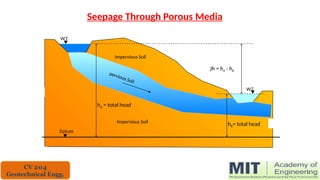
hA = total head
W.T.
)h = hA - hB
W.T.
Impervious Soil
Impervious Soil
pervious Soil
hB= total head
Seepage Through Porous Media
CV 204
Geotechnical Engg.

3. A
B
Soil
Water In
)h =hA - hB
Head Loss or
Head Difference or
Energy Loss
hA
hB
i = Hydraulic Gradient
(q)
Water
out
L = Drainage Path
Datum
hA
W.T.
hB
)h = hA - hB
W.T.
Impervious Soil
Impervious Soil
ZA
Datum
ZB
Elevation
Head
Pressure
Head
Pressure
Head
Elevation
Head
Total
Head
Total
Head
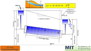
q = v . A = k i A = k A Dh
L
CV 204
Geotechnical Engg.

4. FLOW NETS
Bernoulli's Equation
2g
v
γ
p
z
h
2
w



Elevation Head, m
Fluid Pressure Head, m
Velocity Head, m
water travels very slowly through
soil as opposed to channel flow
0
Total Head, m
CV 204
Geotechnical Engg.

5. FLOW NETS
Bernoulli's Equation
For Seepage through soil:
w
γ
u
z
h 

Pore Water Pressure, kPa
CV 204
Geotechnical Engg.

6. To determine the rate of flow, two parameters are needed
* k = coefficient of permeability
* i = hydraulic gradient
k can be determined using
1- Laboratory Testing [constant head test & falling head test]
2- Field Testing [pumping from wells]
3- Empirical Equations
i can be determined
1- from the head loss
2- flow net
CV 204
Geotechnical Engg.

7. Direction of Flow
Rate of Discharge = qin
X
dZ
Y
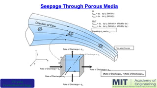
Seepage Through Porous Media
Rate of Discharge = qout
Rate of Discharge = qout
Rate of Discharge = qin
Rate of Discharge = qin
Rate of Discharge = qin
dy
dx
(Rate of Discharge)in = (Rate of Discharge)out
IN
qx(in) = dz . dy kx (Mh/Mx)
qx(in) = dx . dz ky (Mh/My)
OUT
qx (out) = dz . dy kx (Mh/Mx + M2
h/Mx2
dx )
qx (out) = dx . dz ky (Mh/My + M2
h/My2
dy )
Equating q in and q out
Z
Two sets of curves
CV 204
Geotechnical Engg.

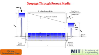
8. Water In
)h =hA - hB
Head Loss or
Head Difference or
Energy Loss
hA
hB
A B
Datum
Porous
Stone
Porous
Stone
Seepage Through Porous Media
i = Hydraulic Gradient
Soil
Water
out
L = Drainage Path
L
CV 204
Geotechnical Engg.

9. Seepage Through Porous Media
Water In
)h =hA - hB
Head Loss or
Head Difference or
Energy Loss
ZA
hB
A B
Datum
Porous
Stone
Porous
Stone
i = Hydraulic Gradient
Soil
Water
out
L = Drainage Path
L
hA
ZB
CV 204
Geotechnical Engg.

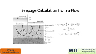
10. Water Flow in a Porous Medium
Goal: Determine the permeability of the
engineering material
Porosity Permeability
Permeability (def) the ease at
which water can move through
rock or soil
Porosity (def) % of
total rock that is
occupied by voids.
CV 204
Geotechnical Engg.

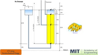
11. 14 ft
3 ft
12 ft
In
Flow
Out
Flow
2 ft
4 ft
Datum
3 ft
3 ft
8 ft
Piezometer
A
B
C
D
u
=
6
x
62.4
u
=
14
x
62.4
No Seepage
Buoyancy
Ws
Ws
Ws
Ws
Ws
CV 204
Geotechnical Engg.

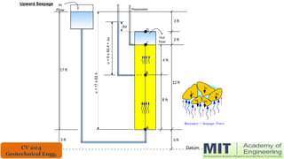
12. 17 ft
3 ft
12 ft
In
Flow
Out
Flow
2 ft
4 ft
Datum
3 ft
3 ft
8 ft
Piezometer
A
B
C
D
u
=
6
x
62.4
+
Du
Du
u
=
17
x
62.4
Upward Seepage
Buoyancy + Seepage Force
Ws
Ws
Ws
Ws
Ws
CV 204
Geotechnical Engg.

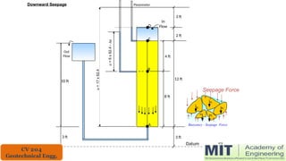
13. 10 ft
3 ft
12 ft
In
Flow
Out
Flow
2 ft
4 ft
Datum
3 ft
3 ft
8 ft
Piezometer
A
B
C
D
u
=
6
x
62.4
-
Du
u
=
17
x
62.4
Downward Seepage
Buoyancy - Seepage Force
Ws
Ws
Ws
Ws
Ws
Seepage Force
CV 204
Geotechnical Engg.

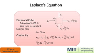
14. Laplace’s Equation
Elemental Cube:
Saturation S=100 %
Void ratio e= constant
Laminar flow
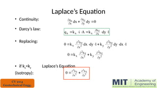
Continuity:
0
dy
q
dx
q
q
q y
q
y
x
q
x
y
x
y
x 





 



 



0
dy
dx y
q
x
q y
x 
 



out
in q
q 
x
q dx
q x
q
x
x



dy
q y
q
y
y



y
q
dx
dy
CV 204
Geotechnical Engg.

15. Laplace’s Equation
• Continuity:
• Darcy’s law:
• Replacing:
• if kx=ky Laplace’s Equation
(isotropy):
0
dy
dx y
q
x
q y
x 
 



1
dy
k
A
i
k
q x
h
x
x
x
T 





 

1
dx
dy
k
1
dy
dx
k
0 2
T
2
2
T
2
y
h
y
x
h
x 











2
T
2
2
T
2
y
h
y
x
h
x k
k
0








2
T
2
2
T
2
y
h
x
h
0






CV 204
Geotechnical Engg.

16. Laplace’s Equation
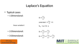
• Typical cases
– 1 Dimensional:
linear variation!!
– 2-Dimensional:
– 3-Dimensional:
2
T
2
x
h
0



i
t
tan
cons x
hT

 

x
b
a
hT 


2
T
2
2
T
2
y
h
x
h
0






2
T
2
2
T
2
2
T
2
z
h
y
h
x
h
0









CV 204
Geotechnical Engg.

17. Laplace’s Equation Solutions
• Exact solutions (for simple B.C.’s)
• Physical models (scaling problems)
• Approximate solutions: method of fragments
• Graphical solutions: flow nets
• Analogies: heat flow and electrical flow
• Numerical solutions: finite differences
CV 204
Geotechnical Engg.

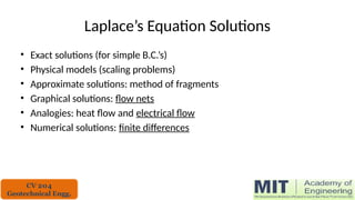
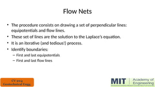
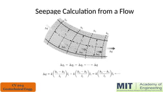
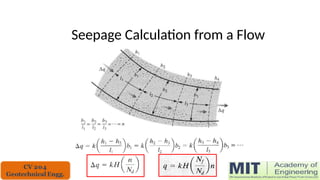
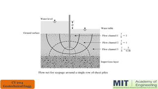
18. Flow Nets
• The procedure consists on drawing a set of perpendicular lines:
equipotentials and flow lines.
• These set of lines are the solution to the Laplace’s equation.
• It is an iterative (and tedious!) process.
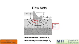
• Identify boundaries:
– First and last equipotentials
– First and last flow lines
CV 204
Geotechnical Engg.

19. Flow Lines
Equipotential Lines
Flow Element
Flow Lines
Principles of the Flow Net

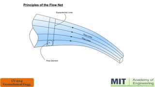
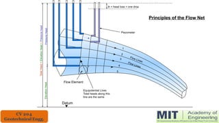
20. Principles of the Flow Net
Flow Lines
Flow Lines
Piezometer
)h = head loss = one drop
Datum
Total
Head
=
Elevation
head
+
Pressure
head
Elevation
Head
Pressure
Head
1
2
3
4
5
Equipotential Lines
Total heads along this
line are the same
Flow Element

21. 8
2
7
6
5
3
4
1
2
)h
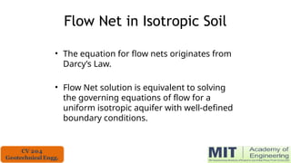
u = [14 - (3. )h)].(water
14 in
Feff = *(soil + * (water - ( - )h) * (water
)h
)h
)h
)h
)h
)h
)h
3 in
2 in
Buoyancy + Seepage Force
Ws
Ws
Ws
Ws
Ws
In
Flow
Out
Flow

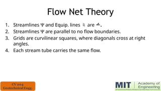
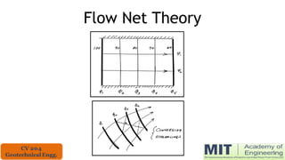
22. Flow Net Theory
1. Streamlines Y and Equip. lines  are .
2. Streamlines Y are parallel to no flow boundaries.
3. Grids are curvilinear squares, where diagonals cross at right
angles.
4. Each stream tube carries the same flow.

23. Flow Net Theory

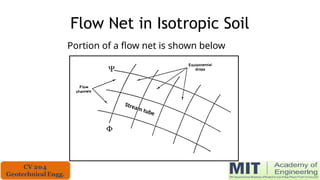
24. Flow Net in Isotropic Soil
Portion of a flow net is shown below
F
Y
Stream tube

25. Flow Net in Isotropic Soil
• The equation for flow nets originates from
Darcy’s Law.
• Flow Net solution is equivalent to solving
the governing equations of flow for a
uniform isotropic aquifer with well-defined
boundary conditions.

26. Flow Net in Isotropic Soil
• Flow through a channel between
equipotential lines 1 and 2 per unit
width is:
∆q = K(dm x 1)(∆h1/dl)
dm
Dh1
dl
F1
F3
Dq
F2
Dh2
Dq
n
m

27. Flow Net in Isotropic Soil
• Flow through equipotential lines 2 and 3 is:
∆q = K(dm x 1)(∆h2/dl)
• The flow net has square grids, so the head
drop is the same in each potential drop:
∆h1 = ∆h2
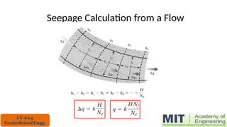
• If there are nd such drops, then:
∆h = (H/n)
where H is the total head loss between the
first and last equipotential lines.

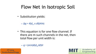
28. Flow Net in Isotropic Soil
• Substitution yields:
– ∆q = K(dm x dl)(H/n)
• This equation is for one flow channel. If
there are m such channels in the net, then
total flow per unit width is:
– q = (m/n)K(dm/dl)H

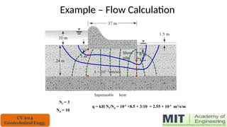
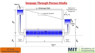
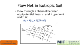
29. Flow Net in Isotropic Soil
• Since the flow net is drawn with squares,
then dm  dl, and:
q = (m/n)KH [L2
T-1
]
where:
– q = rate of flow or seepage per unit width
– m= number of flow channels
– n= number of equipotential drops
– h = total head loss in flow system
– K = hydraulic conductivity

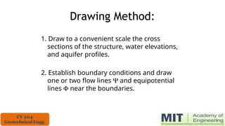
30. Drawing Method:
1. Draw to a convenient scale the cross
sections of the structure, water elevations,
and aquifer profiles.
2. Establish boundary conditions and draw
one or two flow lines Y and equipotential
lines F near the boundaries.

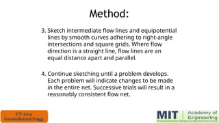
31. Method:
3. Sketch intermediate flow lines and equipotential
lines by smooth curves adhering to right-angle
intersections and square grids. Where flow
direction is a straight line, flow lines are an
equal distance apart and parallel.
4. Continue sketching until a problem develops.
Each problem will indicate changes to be made
in the entire net. Successive trials will result in a
reasonably consistent flow net.

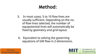
32. Method:
5. In most cases, 5 to 10 flow lines are
usually sufficient. Depending on the no.
of flow lines selected, the number of
equipotential lines will automatically be
fixed by geometry and grid layout.
6. Equivalent to solving the governing
equations of GW flow in 2-dimensions.

33. Seepage Calculation from a Flow
Net

34. Seepage Calculation from a Flow
Net

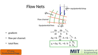
35. Flow Nets
• gradient:
• flow per channel:
• total flow:
Flow channel
Equipotential lines b= l
a
q
h= equipotential drop
b
b
h
l
h
i e
N
h






A
b
k
A
l
h
k
q e
N
h









e
f
f
N
N
b
a
h
k
N
q
q 







36. Flow Nets
Number of flow Channels Nf
Number of potential drops Nd

37. Seepage Calculation from a Flow
Net

38. Seepage Calculation from a Flow
Net

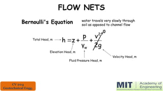
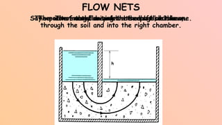
39. FLOW NETS
Say we constructed a tank in the lab like this one.
The water would seep from the left chamber,
through the soil and into the right chamber.
The energy driving the seepage, h?
The path of the flow would be curved as shown.
h

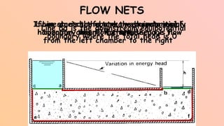
40. FLOW NETS
If we stretch the tank, we have a mainly
horizontal channel for the seepage flow
from the left chamber to the right
h
Lines ab and cefd are the boundaries of
this flow channel
Line ca is the upstream equipotential
boundary where the total head is h
Line bd is the downstream equipotential
boundary where the total head is 0

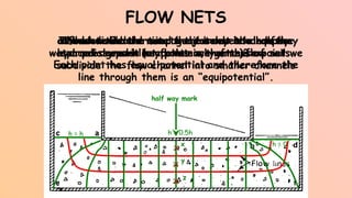
41. FLOW NETS
In order to determine the total head and pore
water pressure at any point in the mass of soil we
subdivide the flow channel into smaller channels
at ca h = h
h = h
at bd h = 0
What would the total head be at the half way
mark (at points x, y or z)?
half way mark
x
y
z
h = 0.5h
The water would rise to the same level on the
hydraulic grade line from each of these points.
Each point has equal potential and therefore the
line through them is an “equipotential”.
h = 0
If we divide the seepage journey into equally
spaced drops in head then we get a flow net.

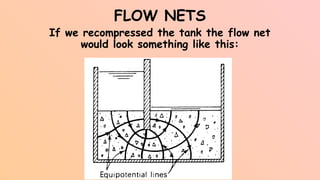
42. FLOW NETS
If we recompressed the tank the flow net
would look something like this:

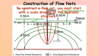
43. Construction of Flow Nets
1. Draw Flow Channel Boundaries 2. Draw Equipotential Boundaries
Upstream Equipotential Boundary
Downstream Equipotential
Boundary
To construct a flow net, you must start
with a scale drawing of the hydraulic
structure:

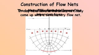
44. Construction of Flow Nets
The first trial:
Not all elements are “square”
The bottom flow channel intersects the
impervious layer
It may take several iterations to finally
come up with a satisfactory flow net.

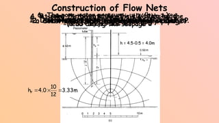
45. And the final version is:
Construction of Flow Nets
To determine the total head at any point, P
2. Show the total head, h driving seepage.
h = 4.5-0.5 = 4.0m
1. Downstream free water surface is datum.
3. Number equipotentials as shown:
4. At point P, the total head is 10/12ths of the
head driving the seepage
3.33m
12
10
4.0
hP 


5. Using the given scale, the elevation head,
zP is -5.2 m
6. The pore water pressure, uP = (hp – zp)w
=(3.33+5.2)x9.8 = 83.3 kPa

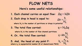
46. FLOW NETS
Here’s some useful relationships:
2. Each drop in head is equal to:
d
N
h
Δh 
where Nd is the number of partitions or drops in potential
1. Each channel carries an equal flow: ∆q = k∆h
3. The total flow carried: q = Nf∆q
where Nf is the number of flow channel partitions
4. Or, the total flow carried:
d
f
N
N
kh
q 
5. And, the head at any point P: h
N
n
h
d
d
p 
where nd is equipotential number (0 at downstream FWS)

47. Clay dam, with air entry
Shale
clay
reservoir
drain

48. Clay dam, with air entry
Shale
clay
reservoir
drain

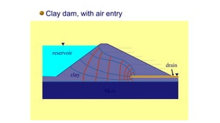
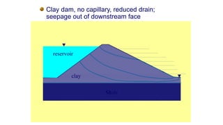
49. Clay dam, no capillary, reduced drain;
seepage out of downstream face
Shale
clay
reservoir

50. Clay dam, no capillary, reduced drain;
seepage out of downstream face
Shale
clay
reservoir

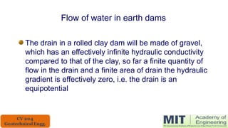
51. Flow of water in earth dams
The drain in a rolled clay dam will be made of gravel,
which has an effectively infinite hydraulic conductivity
compared to that of the clay, so far a finite quantity of
flow in the drain and a finite area of drain the hydraulic
gradient is effectively zero, i.e. the drain is an
equipotential

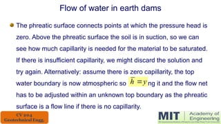
52. The phreatic surface connects points at which the pressure head is
zero. Above the phreatic surface the soil is in suction, so we can
see how much capillarity is needed for the material to be saturated.
If there is insufficient capillarity, we might discard the solution and
try again. Alternatively: assume there is zero capillarity, the top
water boundary is now atmospheric so along it and the flow net
has to be adjusted within an unknown top boundary as the phreatic
surface is a flow line if there is no capillarity.
Flow of water in earth dams
y
h 

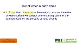
53. If then in the flow net, so once we have the
phreatic surface we can put on the starting points of the
equipotentials on the phreatic surface directly
Flow of water in earth dams
y
h  cons
y
h 



56. Example – Flow Calculation
Nf = 3
Nd = 10
q = kH Nf/Nd = 10-5
×8.5 × 3/10 = 2.55 × 10-5
m3
/s/m

57. Thank You
!!