This document solves a fluid mechanics problem involving compressible one-dimensional flow. It estimates (a) the Mach number at section 1 of a pipe and (b) the pressure inside a tank. It first calculates the Mach number M2 and conditions at section 2, using isentropic nozzle flow equations. It then uses the Fanno flow equation to calculate the maximum possible length Lmax1. Finally, it calculates the Mach number M1 at section 1 and the stagnation pressure and pressure inside the tank.

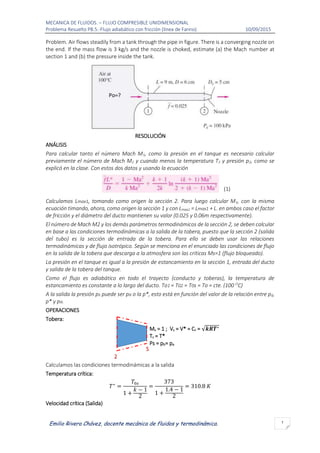
1. MECANICA DE FLUIDOS. – FLUJO COMPRESIBLE UNIDIMENSIONAL
Problema Resuelto P8.5.-Flujo adiabático con fricción (línea de Fanno) 10/09/2015
1
Emilio Rivera Chávez, docente mecánica de fluidos y termodinámica.
Problem. Air flows steadily from a tank through the pipe in figure. There is a converging nozzle on
the end. If the mass flow is 3 kg/s and the nozzle is choked, estimate (a) the Mach number at
section 1 and (b) the pressure inside the tank.
RESOLUCIÓN
ANÁLISIS
Para calcular tanto el número Mach M1, como la presión en el tanque es necesario calcular
previamente el número de Mach M2 y cuando menos la temperatura T2 y presión p2, como se
explicó en la clase. Con estos dos datos y usando la ecuación
(1)
Calculamos Lmax1, tomando como origen la sección 2. Para luego calcular M1, con la misma
ecuación timando, ahora, como origen la sección 1 y con Lmax2 = Lmax1 + L. en ambos caso el factor
de fricción y el diámetro del ducto mantienen su valor (0.025 y 0.06m respectivamente).
El número de Mach M2 y los demás parámetros termodinámicos de la sección 2, se deben calcular
en base a las condiciones termodinámicas a la salida de la tobera, puesto que la sección 2 (salida
del tubo) es la sección de entrada de la tobera. Para ello se deben usar las relaciones
termodinámicas y de flujo isotrópico. Según se menciona en el enunciado las condiciones de flujo
en la salida de la tobera que descarga a la atmosfera son las criticas Ms=1 (flujo bloqueado).
La presión en el tanque es igual a la presión de estancamiento en la sección 1, entrada del ducto
y salida de la tobera del tanque.
Como el flujo es adiabático en todo el trayecto (conducto y toberas), la temperatura de
estancamiento es constante a lo largo del ducto. To1 = T02 = T0s = To = cte. (100 O
C)
A la salida la presión ps puede ser pa o la p*, esto está en función del valor de la relación entre p0,
p* y pa.
OPERACIONES
Tobera:
Ms = 1 ; Vs = V* = Cs = √𝒌𝑹𝑻∗
Ts = T*
Ps = pb= pa
Calculamos las condiciones termodinámicas a la salida
Temperatura crítica:
𝑇∗
=
𝑇0𝑠
1 +
𝑘 − 1
2
=
373
1 +
1.4 − 1
2
= 310.8 𝐾
Velocidad crítica (Salida)
S
2
Po=?

2. MECANICA DE FLUIDOS. – FLUJO COMPRESIBLE UNIDIMENSIONAL
Problema Resuelto P8.5.-Flujo adiabático con fricción (línea de Fanno) 10/09/2015
2
Emilio Rivera Chávez, docente mecánica de fluidos y termodinámica.
V* = Cs = √𝑘𝑅𝑇∗ = √1.4 ∙ 287 ∙ 310.8= 353.38 m/s
Densidad del aire a la salida de la tobera.
𝜌𝑠 =
𝑚
𝐴𝑠 ∙ 𝑉
𝑠
=
3
𝜋 ∙ 0.0252 ∗ 353,38
= 4,234 𝑘𝑔/𝑚3
Presión critica
𝑝∗
= 𝜌∗
𝑅𝑇∗
= 4,234 ∗ 0,287 ∗ 310.8 = 377,67 𝑘𝑃𝑎
Como p* > pa  ps = p*= 377,67 kPa
Presión de estancamiento
𝑝𝑜𝑠 = 𝑝𝑠 (1 +
𝑘 − 1
2
)
𝑘
𝑘−1
= 377,67 (1 +
1.4 − 1
2
)
1.4
1.4−1
= 714,90 𝑘𝑃𝑎
Calculamos ahora las condiciones termodinámicas a la entrada de la tobera
Para esto usamos las ecuaciones fundamentales de flujo, para flujo permanente e isentropico en
la tobera;
Presión y temperatura de estancamiento
Como el flujo en la tobera se considera isentrópico la presión de estancamiento al igual que la
temperatura de estancamiento son constantes a lo largo de la tobera, decir que
p02=p0S=714.90 kPa y T02 = Tos=373 K
Temperatura y presión estáticas
La temperatura y presión a la entrada de la tobera en función de las condiciones de estancamiento
y el número de Mach, están dadas por
𝑻𝟐 =
𝑻𝒐𝟐
(𝟏+
𝒌−𝟏
𝟐
𝑴𝟐
𝟐)
=
𝟑𝟕𝟑
(𝟏+𝟎.𝟐𝑴𝟐
𝟐)
; 𝒑𝟐 =
𝒑𝒐𝟐
(𝟏+
𝒌−𝟏
𝟐
𝑴𝟐
𝟐)
𝒌
𝒌−𝟏
=
𝟕𝟏𝟒,𝟗∗𝟏𝟎𝟑
(𝟏+𝟎.𝟐𝑴𝟐
𝟐)
𝟑.𝟓 (2)
Numero de Mach M2.-
De la ecuación de continuidad  m2=ms = 3 kg/s = cte.
Entonces podemos escribir para la entrada a la tobera:
𝝆𝟐𝑽𝟐𝑨𝟐 = 𝟑
De donde;
3
𝐴2
= 𝜌2𝑉2 = 𝜌2𝑀2√𝑘𝑅𝑇2 =
𝑝2
𝑅𝑇2
𝑀2√𝑘𝑅𝑇2 = 𝑝2𝑀2√
𝑘
𝑅𝑇2
(3)
Combinado (3) con las ecuaciones (2), sustituyendo valores numéricos y operando, se tiene la
siguiente ecuación para M2
3
𝜋 ∙ 0.032
=
714,9 ∗ 103
(1 + 0.2𝑀2
2)3.5
𝑀2
√
𝑘
𝑅
(1 + 0.2𝑀2
2)
373
= 714,90 ∗ 103
∗ √
1.4
287
1
373
𝑀2(1 + 0.2𝑀2
2)−3
𝑀2 = 0,410(1 + 0.2𝑀2
2)3
(3a)

3. MECANICA DE FLUIDOS. – FLUJO COMPRESIBLE UNIDIMENSIONAL
Problema Resuelto P8.5.-Flujo adiabático con fricción (línea de Fanno) 10/09/2015
3
Emilio Rivera Chávez, docente mecánica de fluidos y termodinámica.
Mediante una solución numérica de la ecuación (3a)  M2 ≈ 0,46
Una vez calculado el valor de M2, podemos calcular T2, y p2 con las ecuaciones (1).
𝑻𝟐 =
𝟑𝟕𝟑
(𝟏 + 𝟎. 𝟐𝑴𝟐
𝟐
)
=
𝟑𝟕𝟑
(𝟏 + 𝟎. 𝟐 ∙ 𝟎, 𝟒𝟔𝟐)
= 𝟑𝟓𝟖 𝑲
𝒑𝟐 =
𝟕𝟏𝟒, 𝟗
(𝟏 + 𝟎. 𝟐𝑴𝟐
𝟐
)
𝟑.𝟓
=
𝟕𝟏𝟒, 𝟗
(𝟏 + 𝟎. 𝟐 ∙ 𝟎, 𝟒𝟔𝟐)𝟑.𝟓
= 𝟔𝟏𝟖 𝒌𝑷𝒂
Con los datos calculados de M2, p2 y T2, podemos considerar ahora el conducto recto, para calcular
M1, p01 (presión de estancamiento a la entrada de la tobera y por tanto igual a la presión en el
tanque), tal como lo planificado, líneas arriba.
Cálculo de Lmax1
Aplicando la ecuación 1, entre las secciones 2 y 3 del conducto, se tiene
0,025 ∙ 𝐿𝑚𝑎𝑥1
0,06
=
1 − 0,462
1.4 ∙ 0,462
+
1.4 + 1
2 ∗ 1.4
𝑙𝑛 [
(1.4 + 1) ∙ 0,462
2 + (1.4 − 1) ∙ 0,462
]
Lmax1= 1.4509*0,06/0.025 = 3,48 m
Cálculo de M1
Aplicamos nuevamente, la formula (1), pero ahora entre las secciones 1 y 3, del conducto recto, y
dela relación resultante despejamos M1,
0,025 ∙ 12,48
0,06
=
1 − 𝑀1
2
1.4 ∙ 𝑀1
2 +
1.4 + 1
2 ∗ 1.4
𝑙𝑛 [
(1.4 + 1) ∙ 𝑀1
2
2 + (1.4 − 1) ∙ 𝑀1
2]
5,2 =
1 − 𝑀1
2
1.4 ∙ 𝑀1
2 + 0,857𝑙𝑛 [
2,4 ∙ 𝑀1
2
2 + 0,4 ∙ 𝑀1
2] (4)
M1 = 0,3023 ≈ 0,30 (sol aprox., usando un método numérico)
Presión en el interior del tanque
Como ya mencionamos, la presión en el interior del tanque es igual a la presión de estancamiento
a la salida de la boquilla del mismo que es a su vez la entrada al ducto (sección 1 del ducto), esto
debido a que este flujo, en la boquilla del tanque, puede considerarse isentrópico, por lo que p0=
p01.
Para esto, calculamos previamente p1, podemos hacerlo usando la ecuación del gas ideal,
𝑝1 = 𝜌1𝑅𝑇1
Donde, ve que es necesario calcular previamente 𝑇1 𝑦 𝜌1 , la temperatura T1 se puede calcular
usando la relación entre temperaturas de estancamiento y estática. Asi,
9
1 2 3
M=1
Lmax1
1 2 3
M=1
Lmax1
Lmax2=9 + 3,48 = 12,48

4. MECANICA DE FLUIDOS. – FLUJO COMPRESIBLE UNIDIMENSIONAL
Problema Resuelto P8.5.-Flujo adiabático con fricción (línea de Fanno) 10/09/2015
4
Emilio Rivera Chávez, docente mecánica de fluidos y termodinámica.
𝑻𝟏 =
𝑻𝒐𝟏
(𝟏 +
𝒌 − 𝟏
𝟐
𝑴𝟏
𝟐
)
=
𝟑𝟕𝟑
(𝟏 + 𝟎. 𝟐 ∙ 𝟎, 𝟑𝟐)
= 𝟑𝟔𝟔, 𝟒 𝑲
En cambio para la densidad ρ1, cambiamos de estrategia, la calculamos a partir de la ecuación de
continuidad (en la que no interviene la fricción), pues al no conocer la densidad de estancamiento
no es posible usar la relación matemática entre las densidades de estancamiento y estática como
en el caso de la temperatura.,
𝝆𝟏𝑽𝟏 = 𝝆𝟐𝑽𝟐
Combinamos esta ecuación con relaciones conocidas entre la velocidad, velocidad del sonido y el
número de Mach, para obtener:
𝝆𝟏 = 𝝆𝟐
𝑽𝟐
𝑽𝟏
= (
𝒑𝟐
𝑹 ∙ 𝑻𝟐
) (
𝑴𝟐
𝑴𝟏
√
𝑻𝟐
𝑻𝟏
) = (
𝟔𝟏𝟖
𝟎. 𝟐𝟖𝟕 ∙ 𝟑𝟓𝟖
) (
𝟎, 𝟒𝟔
𝟎, 𝟑𝟎
√
𝟑𝟓𝟖
𝟑𝟔𝟔, 𝟒
) = 𝟗𝟏, 𝟐
𝒌𝒈
𝒎𝟑
𝑝1 = 9,12 ∗ 0,287 ∗ 366,4 = 959,0 𝑘𝑃𝑎
Presión de estancamiento.
Con M1 y p1, se puede calcular la presión de estancamiento en la sección 1, usand loa
relación de presiones estática y de estancamiento,
𝒑𝟎𝟏 = 𝒑𝟏 (𝟏 +
𝒌 − 𝟏
𝟐
𝑴𝟏
𝟐
)
𝒌
𝒌−𝟏
= 𝟗𝟓𝟗 (𝟏 +
𝟏. 𝟒 − 𝟏
𝟐
𝟎, 𝟑𝟐
)
𝟏.𝟒
𝟏.𝟒−𝟏
= 𝟏𝟎𝟐𝟏 𝒌𝑷𝒂
Entonces, como ya se mencionó, la presión en el tanque es:
𝒑𝟎 = 𝒑𝟎𝟏 = 𝟏𝟎𝟐𝟏, 𝟎 𝒌𝑷𝒂
ANEXO
Solución gráfica y por el método de las aproximaciones sucesivas de la ecuación (3a)
𝑀2 = 0,410(1 + 0.2𝑀2
2)3
Grafica que muestra la intersección APROXIMACIONES SUCESIVAS
Ma Mc lMcMal/Ma
0,3 0,433 44,18%
0,433 0,458 5,84%
0,458 0,464 1,31%
0,464 0,465 0,32%
0,465 0,466 0,08%
0,466 0,466 0,02%
Se asume M2 ≈ 0,46 (error ≈1.3 %)
0,2
0,3
0,4
0,5
0,6
0,7
0,8
0,9
0,2 0,3 0,4 0,5 0,6 0,7 0,8 0,9
Solucion gráfica
Numero de Mach M2