Flow net unde Homogenous Earthern Dam part 1

1. FLOW NETS

2. Techniques for Finding “Solutions” to
Groundwater Flow”

3. Techniques for Finding “Solutions” to
Groundwater Flow”
• Inspection (intuition)
• Graphical Techniques

4. Techniques for Finding “Solutions” to
Groundwater Flow”
• Inspection (intuition)
• Graphical Techniques
• Analog Models

5. Techniques for Finding “Solutions” to
Groundwater Flow”
• Inspection (intuition)
• Graphical Techniques
• Analog Models
• Analytical Mathematical Techniques
(Calculus)

6. Techniques for Finding “Solutions” to
Groundwater Flow”
• Inspection (intuition)
• Graphical Techniques
• Analog Models
• Analytical Mathematical Techniques (Calculus)
• Numerical Mathematical Techniques
(Computers)

7. I. Introduction
A. Overview

8. I. Introduction
A. Overview
• one of the most powerful tools for the
analysis of groundwater flow.

9. I. Introduction
A. Overview
• one of the most powerful tools for the
analysis of groundwater flow.
• provides a solution to LaPlaces
Equation for 2-D, steady state,
boundary value problem.

10. I. Introduction
A. Overview
• one of the most powerful tools for the analysis of groundwater
flow.
• provides a solution to LaPlaces Equation for 2-D, steady state,
boundary value problem.
• To solve, need to know:

11. I. Introduction
A. Overview
• one of the most powerful tools for the analysis of groundwater
flow.
• provides a solution to LaPlaces Equation for 2-D, steady state,
boundary value problem.
• To solve, need to know:
– have knowledge of the region of flow

12. I. Introduction
A. Overview
• one of the most powerful tools for the analysis of groundwater
flow.
• provides a solution to LaPlaces Equation for 2-D, steady state,
boundary value problem.
• To solve, need to know:
– have knowledge of the region of flow
– boundary conditions along the perimeter of
the region

13. • To solve, need to know:
– have knowledge of the region of flow
– boundary conditions along the perimeter of
the region
– spatial distribution of hydraulic head in
region.

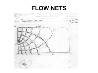
14. • Composed of 2 sets of lines
– equipotential lines (connect points of equal
hydraulic head)
– flow lines (pathways of water as it moves
through the aquifer.

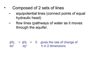
15. • Composed of 2 sets of lines
– equipotential lines (connect points of equal
hydraulic head)
– flow lines (pathways of water as it moves
through the aquifer.
d2
h + d2
h = 0 gives the rate of change of
dx2
dy2
h in 2 dimensions

16. II. Assumptions Needed For Flow Net
Construction

17. II. Assumptions Needed For Flow Net
Construction
• Aquifer is homogeneous, isotropic
• Aquifer is saturated

18. II. Assumptions Needed For Flow Net
Construction
• Aquifer is homogeneous, isotropic
• Aquifer is saturated
• There is no change in head with time

19. II. Assumptions Needed For Flow Net
Construction
• Aquifer is homogeneous, isotropic
• Aquifer is saturated
• There is no change in head with time
• Soil and water are incompressible

20. II. Assumptions Needed For Flow Net
Construction
• Aquifer is homogeneous, isotropic
• Aquifer is saturated
• there is no change in head with time
• soil and water are incompressible
• Flow is laminar, and Darcys Law is valid

21. II. Assumptions Needed For Flow Net
Construction
• Aquifer is homogeneous, isotropic
• Aquifer is saturated
• there is no change in head with time
• soil and water are incompressible
• flow is laminar, and Darcys Law is valid
• All boundary conditions are known.

22. III. Boundaries

23. III. Boundaries
A. Types

24. III. Boundaries
A. Types
1. Impermeable
2. Constant Head
3. Water Table

25. III. Boundaries
A. Types
1. Impermeable
2. Constant Head
3. Water Table

26. III. Boundaries
B. Calculating Discharge Using Flow Nets
Q’ = Kph
f
Where:
Q’ = Discharge per unit depth of flow net (L3/t/L)
K = Hydraulic Conductivity (L/t)
p = number of flow tubes
h = head loss (L)
f = number of equipotential drops

27. IV. Refraction of Flow Lines

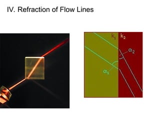
28. IV. Refraction of Flow Lines
A. The derivation
B. The general relationships
C. An example problem

29. IV. Flow Nets: Isotropic, Heterogeneous
Types
A. “Reminder” of the conditions needed to
draw a flow net for homogeneous,
isotropic conditions
B. An Example of Iso, Hetero