Searching and Sorting Algorithms

Searching and Sorting Algorithms
Dr. Ashutosh Satapathy
Assistant Professor, Department of CSE
VR Siddhartha Engineering College
Kanuru, Vijayawada
March 9, 2024
Dr. Ashutosh Satapathy Searching and Sorting Algorithms March 9, 2024 1 / 73

Outline
1 Searching
Introduction
Linear Search
Binary Search
2 Sorting
Introduction
Insertion Sort
Selection Sort
Bubble Sort
Optimized Bubble Sort

Outline
1 Searching
Introduction
Linear Search
Binary Search
2 Sorting
Introduction
Insertion Sort
Selection Sort
Bubble Sort

Introduction
Information retrieval is one of the important applications of
computers. It becomes necessary to search a list of records to identify
a particular record.
Each record contains a field whose value is unique to distinguish
among the records are known as keys.
A particular record can be identified when key value of that record is
equal to a given input value. This operation is known as searching.
If the record is found then search is said to be successful, otherwise it
is unsuccessful. The searching problem falls into two cases.
If there are many records, perhaps each one quite large, then it will be
necessary to store the records in files on disk or tape, external to the
primary memory. This is called external searching.
Else, the records to be searched are stored entirely in the primary
memory. This is called internal searching.

Outline
1 Searching
Introduction
Linear Search
Binary Search
2 Sorting
Introduction
Insertion Sort
Selection Sort
Bubble Sort

Linear Search
The simplest way to do a search is to begin at one end of the list and
scan down it until the desired key is found or the other end is
reached.
Let us assume that a is an array of n keys, a[0] through a[n-1]. Let
us also assume that key is a search element.
The process starts with a comparison between the first element (i.e,
a[0]) and key. As long as a comparison does not result in a success,
the algorithm proceeds to compare the next element of a and key.
The process terminates when the list exhausted or a comparison
results in a success. This method of searching is also known as
linear searching.

Linear Search
Algorithm 1 Linear search
1: procedure linearsearch(a, n, key)
2: for i ← 0 to n − 1 do
3: if (key = a[i]) then
4: return i
5: end if
6: end for
7: return -1
8: end procedure
The function examines each key in turn; upon finding one that
matches the search argument, its index is returned. If no match is
found, -1 is returned.
When the values of the array a are not distinct then the function
will return the first index of the array a which is equal to key.

Linear Search
Best Case Time Complexity: The searched element is available at the
a[0].
Algorithm 2 Linear search best case analysis
1: procedure linearsearch(a, n, key) ▷ Frequency count is 1
2: for i ← 0 to n − 1 do ▷ Frequency count is 1
3: if (key = a[i]) then ▷ Frequency count is 1
4: return i ▷ Frequency count is 1
5: end if ▷ Frequency count is 0
6: end for ▷ Frequency count is 0
7: return -1 ▷ Frequency count is 0
8: end procedure ▷ Frequency count is 0
Total frequency count f(n) is 4. So, the best-case time complexity is
O(1).

Linear Search
Worst Case Time Complexity: The searched element is available at the
a[n-1].
Algorithm 3 Linear search worst case analysis
2: for i ← 0 to n − 1 do ▷ Frequency count is n
3: if (key = a[i]) then ▷ Frequency count is n
6: end for ▷ Frequency count is 0
Total frequency count f(n) is 2n+2. So, the worst-case time complexity
is O(n).

Linear Search
Worst Case Time Complexity: The searched element is is not available
in the array.
Algorithm 4 Linear search worst case analysis
2: for i ← 0 to n − 1 do ▷ Frequency count is n+1
3: if (key = a[i]) then ▷ Frequency count is n
6: end for ▷ Frequency count is n
Total frequency count f(n) is 3n+4. So, the worst-case time complexity
is O(n).

Linear Search
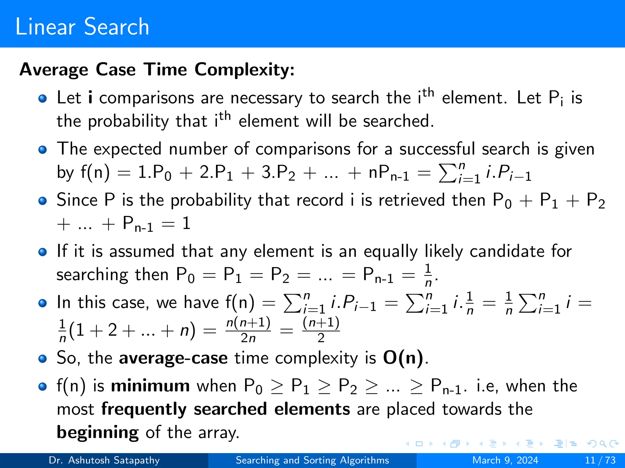
Average Case Time Complexity:
Let i comparisons are necessary to search the ith element. Let Pi is
the probability that ith element will be searched.
The expected number of comparisons for a successful search is given
by f(n) = 1.P0 + 2.P1 + 3.P2 + ... + nPn-1 =
Pn
i=1 i.Pi−1
Since P is the probability that record i is retrieved then P0 + P1 + P2
+ ... + Pn-1 = 1
If it is assumed that any element is an equally likely candidate for
searching then P0 = P1 = P2 = ... = Pn-1 = 1
n .
In this case, we have f(n) =
Pn
i=1 i.Pi−1 =
Pn
i=1 i.1
n = 1
n
Pn
i=1 i =
1
n (1 + 2 + ... + n) = n(n+1)
2n = (n+1)
2
So, the average-case time complexity is O(n).
f(n) is minimum when P0 ≥ P1 ≥ P2 ≥ ... ≥ Pn-1. i.e, when the
most frequently searched elements are placed towards the
beginning of the array.

Linear Search
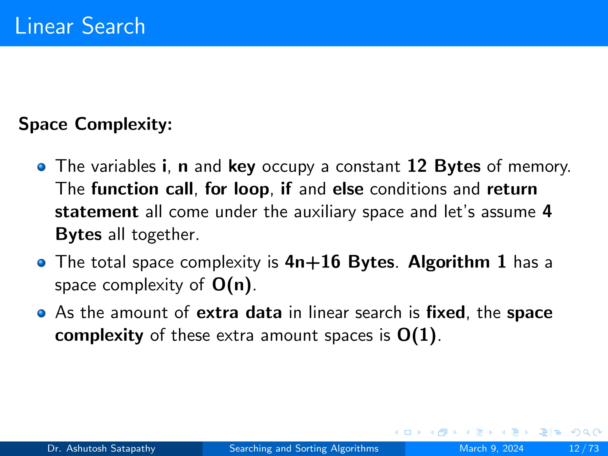
Space Complexity:
The variables i, n and key occupy a constant 12 Bytes of memory.
The function call, for loop, if and else conditions and return
statement all come under the auxiliary space and let’s assume 4
Bytes all together.
The total space complexity is 4n+16 Bytes. Algorithm 1 has a
space complexity of O(n).
As the amount of extra data in linear search is fixed, the space
complexity of these extra amount spaces is O(1).

Outline
1 Searching
Introduction
Linear Search
Binary Search
2 Sorting
Introduction
Insertion Sort
Selection Sort
Bubble Sort

Binary Search
Sequential search is simple method for searching an element in an
array. This is efficient for a small list of elements.
Highly inefficient for larger lists. In the worst case, we will have to
make n comparisons, as to search for the last element in the list.
Binary search is a very efficient search technique which works for
sorted lists.
we make a comparison between key and middle element of array or
identifying the left half or the right half of the array to which the
desired element may belong.
The procedure is repeated on the half in which the desired element
is likely to be present.
When the number of elements is even, there are two elements in the
middle. However, an arbitrary choice of any one of these as the
middle element will serve the purpose.

Binary Search
Algorithm 5 Binary search
1: procedure binarysearch(a, n, key)
2: low ← 0
3: high ← n − 1
4: while (low ≤ high) do
5: mid ←⌈low+high
2 ⌉
6: if (key = a[mid]) then
7: return mid
8: else if (key < a[mid]) then
9: high ← mid − 1
10: else
11: low ← mid + 1
12: end if
13: end while
14: return -1
15: end procedure

Binary Search
Figure 1.1: Search key value 19 in the given set of data using binary search.

Binary Search
Algorithm 6 Binary search best case time complexity - O(1)
1: procedure binarysearch(a, n, key) ▷ Frequency count is 1
2: low ← 0 ▷ Frequency count is 1
3: high ← n − 1 ▷ Frequency count is 1
4: while (low ≤ high) do ▷ Frequency count is 1
5: mid ←⌈low+high
2 ⌉ ▷ Frequency count is 1
6: if (key = a[mid]) then ▷ Frequency count is 1
7: return mid ▷ Frequency count is 1
8: else if (key < a[mid]) then ▷ Frequency count is 0
9: high ← mid − 1 ▷ Frequency count is 0
10: else ▷ Frequency count is 0
11: low ← mid + 1 ▷ Frequency count is 0
13: end while ▷ Frequency count is 0

Binary Search
Worst Case Time Complexity:
To analyze the performance of binary search, the maximum number
of comparisons required for a successful search will be computed.
Let i be the smallest integer such that 2i ≥ n+1.
The maximum number of elements that are left after the first
comparison is 2i-1-1 and in general, the maximum number of
elements left after k comparisons is 2i-k-1.
we are left with no elements to be compared after i comparisons as
2i-i-1.
f(n), the maximum number of comparisons for a successful search is
given by f(n) = i.
So, 2i = n + 1 ⇒ log2 2i = log2(n + 1) ⇒ i log2 2 = log2(n + 1) ⇒
i = log2(n + 1) ⇒ f (n) = log2(n + 1). The worst case time
complexity is O(log2n).
Search can be declared as unsuccessful only when there are no
elements to be probed.

Binary Search
The average number of comparisons under the assumption that
each key is an equally likely candidate for a search.
the probability that a particular element will be requested in a search
is (1/n).
We assume n=2i-1 for some i. Now, the element in middle
position requires only one comparison to be searched.
the elements in the middle positions of the two halves require two
comparisons each when searched.
The total number of comparisons required to search every array
element is given by
C(n) = 1.20
+ 2.21
+ 3.22
+ ... + i.2i-1
(1)
Multiply both sides of equation (2) by 2
2.C(n) = 1.21
+ 2.22
+ 3.23
+ ... + i.2i
(2)

Binary Search
Subtracting equation (2) from equation (3), the result is
C(n) = i.2i − (20 + 21 + 22 + ... + 2i-1) = i.2i −
Pi−1
i=0 2i =
i.2i − 2i + 1 = 1 + 2i (i − 1)
The average number of comparisons for a successful search, is given
by f (n) = C(n)
n = 1+2i (i−1)
n
As 2i = n + 1 ⇒ i = log2(n + 1) ⇒ i − 1 = log2(n + 1) − 1.
f (n) = 1+2i (i−1)
n = 1+(n+1)(log2(n+1)−1)
n = (n+1) log2(n+1)
n − 1
The above outcome has been derived under the assumption that n is
of the form 2i-1, the approximate result is valid for any value of n.
So, the average number of comparisons for a successful as well as
unsuccessful number of comparison are O(log2n).

Binary Search
Space Complexity:
The variables n, key, low, high and mid occupy a constant 20 Bytes
of memory. The function call, while loop, if, else if and else
conditions and return statement all come under the auxiliary space
and let’s assume K Bytes all together.
The total space complexity is 4n+20+K Bytes. Algorithm 5 has a
As the amount of extra variables in binary search is fixed, the space

Outline
1 Searching
Introduction
Linear Search
Binary Search
2 Sorting
Introduction
Insertion Sort
Selection Sort
Bubble Sort

Introduction
Sorting is arranging the data in ascending or descending order.
The term sorting came into picture, as humans realised the
importance of searching quickly.
If an array A contains a sequence of n numbers <a1, a2, ..., an>.
A Sorting is the permutation (reordering) <a1
’, a2
’, ..., an
’> of
the input sequence such that a1
’ ≤ a2
’ ≤ ... ≤ an
’.
Since the beginning of the programming age, computer scientists
have been working on solving the problem of sorting by coming up
with various different algorithms to sort data.
Some of the sorting techniques are Bubble sort, Selection sort,
Insertion sort, Merge sort, Quick sort and Heap sort etc.

Outline
1 Searching
Introduction
Linear Search
Binary Search
2 Sorting
Introduction
Insertion Sort
Selection Sort
Bubble Sort

Insertion Sort
Insertion sort is an efficient algorithm for sorting a small number
of elements. It sorts a set of values by inserting values in to an
existing sorted file.
The method can be explained in the similar way the arrangement of
cards by a card player.
The card player picks up the cards and inserts them in to the
required position.
Thus at every step, we insert an item in to its proper place in an
already ordered list.
suppose an array a with n elements a[0], a[1], ..., a[n-1] is in memory.
The insertion sort scans a from a[0] to a[n-1], inserting each element
a[k] in to its proper position in the previously sorted sub-array
a[0], a[1], ...., a[k-1].

Insertion Sort
Algorithm 7 Insertion Sort
1: procedure insertion-sort(A, n)
2: for j ← 1 to n − 1 do
3: key ← A[j]
4: i ← j-1
5: while (i ≥ 0 and A[i] > key) do
6: A[i+1] ← A[i]
7: i ← i-1
8: end while
9: A[i+1] ← key
10: end for
11: end procedure

Insertion Sort
Figure 2.1: Arrange array elements in ascending order using insertion sort.

Insertion Sort
Best Case Time Complexity:
Algorithm 8 Insertion Sort Best Case Analysis
1: procedure insertion-sort(A, n) ▷ Frequency count is 1
2: for j ← 1 to n − 1 do ▷ Frequency count is n
3: key ← A[j] ▷ Frequency count is n-1
4: i ← j-1 ▷ Frequency count is n-1
5: while (i ≥ 0 and A[i] > key) do ▷ Frequency count is n-1
6: A[i+1] ← A[i] ▷ Frequency count is 0
7: i ← i-1 ▷ Frequency count is 0
8: end while ▷ Frequency count is 0
9: A[i+1] ← key ▷ Frequency count is n-1
10: end for ▷ Frequency count is n-1
Total frequency count f(n) is 6n-3. The best case time complexity is O(n)

Insertion Sort
Table 2.1: Worst case time complexity analysis of Insertion sort.
Statement Frequency Count Time
1 1 O(1)
2 n O(n)
3 n-1 O(n)
4 n-1 O(n)
5 2+3+4+...+n = n(n+1)/2 - 1 O(n2)
6 1+2+3+...+n-1 = n(n-1)/2 O(n2)
7 1+2+3+...+n-1 = n(n-1)/2 O(n2)
8 1+2+3+...+n-1 = n(n-1)/2 O(n2)
9 n-1 O(n)
10 n-1 O(n)
11 1 O(1)
f(n) 2n2+4n-3 O(n2)

Insertion Sort
Best Case Time Complexity Analysis - Big Oh Notation
f(n) = 6n-3 ≤ cn
Assume c = 6, then f(n) = 6n-3 ≤ 6n
⇒ 3 ≤ 6 [Since n0 = 1]
For n0 ≥ 1, f(n) ≤ 6n
So, best case time complexity O(n), where n0 = 1 and c = 6.
Worst Case Time Complexity Analysis - Big Oh Notation
f(n) = 2n2+4n-3 ≤ cn2
Assume c = 3, then f(n) = 2n2+4n-3 ≤ 3n2
⇒ 27 ≤ 27 [Since n0 = 3]
For n0 ≥ 3, f(n) ≤ 3n2
So, worst case time complexity O(n2), where n0 = 3 and c = 3.

Insertion Sort
Best Case Time Complexity Analysis - Big Omega Notation
f(n) = 6n-3 ≥ cn
Assume c = 5, then f(n) = 6n-3 ≥ 5n
⇒ 15 ≥ 15 [Since n0 = 3]
For n0 ≥ 3, f(n) ≥ 5n
So, best case time complexity Ω(n), where n0 = 3 and c = 5.
Worst Case Time Complexity Analysis - Big Omega Notation
f(n) = 2n2+4n-3 ≥ cn2
Assume c = 2, then f(n) = 2n2+4n-3 ≥ 2n2
⇒ 3 ≥ 2 [Since n0 = 1]
For n0 ≥ 1, f(n) ≥ 2n2
So, worst case time complexity Ω(n2), where n0 = 1 and c = 2.

Insertion Sort
Best Case Time Complexity Analysis - Little Oh Notation
f(n) = 6n-3 < cn
Assume c = 6, then f(n) = 6n-3 < 6n
⇒ 3 < 6 [Since n0 = 1]
For n0 ≥ 1, f(n) < 6n
So, best case time complexity o(n), where n0 = 1 and c = 6.
Worst Case Time Complexity Analysis - Little Oh Notation
f(n) = 2n2+4n-3 < cn2
Assume c = 3, then f(n) = 2n2+4n-3 < 3n2
⇒ 45 < 48 [Since n0 = 4]
For n0 ≥ 4, f(n) < 3n2
So, worst case time complexity o(n2), where n0 = 4 and c = 3.

Insertion Sort
Best Case Time Complexity Analysis - Little Omega Notation
f(n) = 6n-3 > cn
Assume c = 5, then f(n) = 6n-3 > 5n
⇒ 21 > 20 [Since n0 = 4]
For n0 ≥ 4, f(n) > 5n
So, best case time complexity ω(n), where n0 = 4 and c = 5.
Worst Case Time Complexity Analysis - Little Omega Notation
f(n) = 2n2+4n-3 > cn2
Assume c = 2, then f(n) = 2n2+4n-3 > 2n2
⇒ 3 > 2 [Since n0 = 1]
For n0 ≥ 1, f(n) > 2n2
So, worst case time complexity ω(n2), where n0 = 1 and c = 2.

Insertion Sort
Best Case Time Complexity Analysis - Theta Notation
c1n ≤ f(n) = 6n-3 ≤ c2n
Assume c1 = 5 and c2 = 6, then 5n ≤ 6n-3 ≤ 6n
⇒ 15 ≤ 15 ≤ 18 [Since n0 = 3]
For n0 ≥ 3, 5n ≤ f(n) ≤ 6n
So, best case time complexity θ(n), where n0 = 3, c1 = 5 and c2 = 6.
Worst Case Time Complexity Analysis - Theta Notation
c1n2 ≤ f(n) = 2n2+4n-3 ≤ c2n2
Assume c1 = 2 and c2 = 3, then 2n2 ≤ 2n2+4n-3 ≤ 3n2
⇒ 18 ≤ 27 ≤ 27 [Since n0 = 3]
For n0 ≥ 3, 2n2 ≤ f(n) ≤ 3n2
So, worst case time complexity θ(n2), where n0 = 3, c1 = 2 and c2 = 3.

Insertion Sort
Space Complexity:
The variables n, key, iand j occupy a constant 16 Bytes of memory.
The function call, while loop and for loop all come under the
auxiliary space and let’s assume K Bytes all together.
As the amount of extra variables in insertion sort is fixed, the space

Outline
1 Searching
Introduction
Linear Search
Binary Search
2 Sorting
Introduction
Insertion Sort
Selection Sort
Bubble Sort

Selection Sort
The selection sort is also known as push-down sort.
The sort consists entirely of a selection phase in which the smallest
of the remaining elements, small, is repeatedly placed in its proper
position.
Let a be an array of n elements. Find the position i of the smallest
element in the list of n elements a[0], a[1], ..., a[n-1] and then
interchange a[i] with a[0]. Then a[0] is sorted.
Find the position i of the smallest in the sub-list of n-1 elements
a[1], a[2], ..., a[n-1]. Then interchange a[i] with a[1]. Then a[0]
and a[1] are sorted.
find the position i of the smallest element in the sub-list of n-2
elements a[2], a[3], ..., a[n-1]. Then interchange a[i] with a[2].
Then a[0], a[1] and a[2] are sorted.
Like this, find the position i of the smallest element between a[n-2]
and a[n-1]. Then interchange a[i] with a[n-2]. Then the array a is
sorted.

Selection Sort
Algorithm 9 Selection Sort
1: procedure Selection-sort(A, n)
2: for i ← 0 to n − 2 do
3: min ← i
4: for j ← i + 1 to n − 1 do
5: if A[j] < a[min] then
6: min ← j // index of the ith smallest element.
7: end if
8: end for
9: t ← A[min]
10: a[min] ← A[i]
11: a[i] ← t
12: end for
13: end procedure

Selection Sort
Figure 2.2: Arrange array elements in ascending order using selection sort.

Selection Sort
Best Case Time Complexity: Total freq. count f(n) is 1.5n2+5.5n-4
1: procedure Selection-sort(A, n) ▷ Frequency count is 1
3: min ← i ▷ Frequency count is n-1
4: for j ← i + 1 to n − 1 do ▷ Freq. count is n(n+1)/2 -1
5: if A[j] < a[min] then ▷ Freq. count is n(n-1)/2
6: min ← j ▷ Frequency count is 0
8: end for ▷ Freq. count is n(n-1)/2
9: t ← A[min] ▷ Frequency count is n-1
10: a[min] ← A[i] ▷ Frequency count is n-1
11: a[i] ← t ▷ Frequency count is n-1

Selection Sort
Worst Case Time Complexity: Total freq. count f(n) is 2.5n2+4.5n-4
1: procedure Selection-sort(A, n) ▷ Frequency count is 1
3: min ← i ▷ Frequency count is n-1
4: for j ← i + 1 to n − 1 do ▷ Freq. count is n(n+1)/2 -1
5: if A[j] < a[min] then ▷ Freq. count is n(n-1)/2
6: min ← j ▷ Freq. count is n(n-1)/2
7: end if ▷ Freq. count is n(n-1)/2
9: t ← A[min] ▷ Frequency count is n-1
10: a[min] ← A[i] ▷ Frequency count is n-1
11: a[i] ← t ▷ Frequency count is n-1

Selection Sort
f(n) = 1.5n2+5.5n-4 ≤ cn2
Assume c = 2, then f(n) = 1.5n2+5.5n-4 ≤ 2n2
⇒ 238 ≤ 242 [Since n0 = 11]
For n0 ≥ 11, f(n) ≤ 2n2
So, best case time complexity O(n2), where n0 = 11 and c = 2.
f(n) = 2.5n2+4.5n-4 ≤ cn2
Assume c = 3, then f(n) = 2.5n2+4.5n-4 ≤ 3n2
⇒ 192 ≤ 192 [Since n0 = 8]
For n0 ≥ 8, f(n) ≤ 3n2

Selection Sort
f(n) = 1.5n2+5.5n-4 ≥ cn2
Assume c = 1, then f(n) = 1.5n2+5.5n-4 ≥ n2
⇒ 3 ≥ 1 [Since n0 = 1]
For n0 ≥ 1, f(n) ≥ n2
So, best case time complexity Ω(n2), where n0 = 1 and c = 1.
f(n) = 2.5n2+4.5n-4 ≥ cn2
Assume c = 2, then f(n) = 2.5n2+4.5n-4 ≥ 2n2
⇒ 3 ≥ 2 [Since n0 = 1]
For n0 ≥ 1, f(n) ≥ 2n2

Selection Sort
f(n) = 1.5n2+5.5n-4 < cn2
Assume c = 2, then f(n) = 1.5n2+5.5n-4 < 2n2
⇒ 238 < 242 [Since n0 = 11]
For n0 ≥ 11, f(n) < 2n2
So, best case time complexity o(n2), where n0 = 11 and c = 2.
f(n) = 2.5n2+4.5n-4 < cn2
Assume c = 3, then f(n) = 2.5n2+4.5n-4 < 3n2
⇒ 239 < 243 [Since n0 = 9]
For n0 ≥ 9, f(n) < 3n2

Selection Sort
f(n) = 1.5n2+5.5n-4 > cn2
Assume c = 1, then f(n) = 1.5n2+5.5n-4 > n2
⇒ 3 > 1 [Since n0 = 1]
For n0 ≥ 1, f(n) > n2
So, best case time complexity ω(n2), where n0 = 1 and c = 1.
f(n) = 2.5n2+4.5n-4 > cn2
Assume c = 2, then f(n) = 2.5n2+4.5n-4 > 2n2
⇒ 3 > 2 [Since n0 = 1]
For n0 ≥ 1, f(n) > 2n2

Selection Sort
c1n2 ≤ f(n) = 1.5n2+5.5n-4 ≤ c2n2
Assume c1 = 1 and c2 = 2, then n2 ≤ 1.5n2+5.5n-4 ≤ 2n2
⇒ 121 ≤ 238 ≤ 242 [Since n0 = 11]
For n0 ≥ 11, n2 ≤ f(n) ≤ 2n2
c1n2 ≤ f(n) = 2.5n2+4.5n-4 ≤ c2n2
Assume c1 = 2 and c2 = 3, then 2n2 ≤ 2.5n2+4.5n-4 ≤ 3n2
⇒ 128 ≤ 192 ≤ 192 [Since n0 = 8]
For n0 ≥ 8, 2n2 ≤ f(n) ≤ 3n2

Selection Sort
Space Complexity:
The variables n, min, t, i and j occupy a constant 20 Bytes of
memory. The function call, while loop and for loop all come under
the auxiliary space and let’s assume K Bytes all together.
As the number of extra variables in the selection sort is fixed, the
space complexity of these extra spaces is O(1).

Outline
1 Searching
Introduction
Linear Search
Binary Search
2 Sorting
Introduction
Insertion Sort
Selection Sort
Bubble Sort

Bubble Sort
Bubble sort proceeds by scanning the list from left to right, and
whenever a pair of adjacent keys found out of order, those
items are swapped.
This process repeats till all the elements of the list are in sorted order.
Let a is an array of n integers in which the elements are to be
sorted, so that a[i] ≤ a[j] for 0 ≤ i < j < n.
The basic idea of bubble sort is to pass through the list sequentially
several times.
Each pass consists of comparing each element in the list with its
successors and interchanging the two elements if they are not in the
proper order.
In Pass 1, Compare a[0] and a[1] and arrange them in order so that
a[0] ≤ a[1]. Then compare a[1] and a[2] and arrange them so that
a[1] ≤ a[2].

Bubble Sort
Continue until a[n-2] and a[n-1] comparison and arrange them so
that a[n-2] ≤ a[n-1]. Pass 1 involves n-1 comparison and the
largest element occupies (n-1)th position.
In Pass 2, repeat the above process with one less comparison i.e.
stop after comparing and possible rearrangement of a[n-3] and
a[n-2].
It involves n-2 comparisons, the second largest element will
occupies (n-2)th position. The process continues, and the (n-i)th
index position receives ith largest element after pass i.
Compare a[0] and a[1] in pass n-1, and arrange them so that a[0]
≤ a[1].

Bubble Sort
Algorithm 12 Bubble Sort
1: procedure Bubble-sort(A, n)
2: for i ← 0 to n − 2 do
3: for j ← 0 to n − i − 2 do
4: // compare adjacent elements
5: if A[j] > a[j + 1] then
6: t ← A[j]
7: a[j] ← A[j + 1]
8: a[j + 1] ← t
9: end if
10: end for
11: end for
12: end procedure

Bubble Sort
Figure 2.3: Array elements after Pass 1 of bubble sort.

Bubble Sort
Figure 2.4: Array elements after Pass 2 of bubble sort.

Bubble Sort
Best Case Time Complexity:
1: procedure Bubble-sort(A, n) ▷ Frequency count is 1
3: for j ← 0 to n − i − 2 do ▷ Freq. count is n(n+1)/2 -1
4: if A[j] > a[j + 1] then ▷ Freq. count is n(n-1)/2
5: t ← A[j] ▷ Frequency count is 0
6: a[j] ← A[j + 1] ▷ Frequency count is 0
7: a[j + 1] ← t ▷ Frequency count is 0
Total frequency count f(n) is 1.5n2+1.5n. The best case time complexity
is O(n2)

Bubble Sort
Worst Case Time Complexity:
1: procedure Bubble-sort(A, n) ▷ Frequency count is 1
3: for j ← 0 to n − i − 2 do ▷ Freq. count is n(n+1)/2 -1
4: if A[j] > a[j + 1] then ▷ Freq. count is n(n-1)/2
5: t ← A[j] ▷ Freq. count is n(n-1)/2
6: a[j] ← A[j + 1] ▷ Freq. count is n(n-1)/2
7: a[j + 1] ← t ▷ Freq. count is n(n-1)/2
8: end if ▷ Freq. count is n(n-1)/2
Total frequency count f(n) is 3.5n2-0.5n. The worst case time complexity
is O(n2)

Bubble Sort
f(n) = 1.5n2+1.5n ≤ cn2
Assume c = 2, then f(n) = 1.5n2+1.5n ≤ 2n2
⇒ 18 ≤ 18 [Since n0 = 3]
For n0 ≥ 3, f(n) ≤ 2n2
So, best case time complexity O(n2), where n0 = 3 and c = 2.
f(n) = 3.5n2-0.5n ≤ cn2
Assume c = 4, then f(n) = 3.5n2-0.5n ≤ 4n2
⇒ 3 ≤ 4 [Since n0 = 1]
For n0 ≥ 1, f(n) ≤ 4n2

Bubble Sort
f(n) = 1.5n2+1.5n ≥ cn2
Assume c = 1, then f(n) = 1.5n2+1.5n ≥ n2
⇒ 3 ≥ 1 [Since n0 = 1]
For n0 ≥ 1, f(n) ≥ n2
So, best case time complexity Ω(n2), where n0 = 1 and c = 1.
f(n) = 3.5n2-0.5n ≥ cn2
Assume c = 3, then f(n) = 3.5n2-0.5n ≥ 3n2
⇒ 3 ≥ 3 [Since n0 = 1]
For n0 ≥ 1, f(n) ≥ 3n2

Bubble Sort
f(n) = 1.5n2+1.5n < cn2
Assume c = 2, then f(n) = 1.5n2+1.5n < 2n2
⇒ 30 < 32 [Since n0 = 4]
For n0 ≥ 4, f(n) < 2n2
f(n) = 3.5n2-0.5n < cn2
Assume c = 4, then f(n) = 3.5n2-0.5n < 4n2
⇒ 3 < 4 [Since n0 = 1]
For n0 ≥ 1, f(n) < 4n2

Bubble Sort
f(n) = 1.5n2+1.5n > cn2
Assume c = 1, then f(n) = 1.5n2+1.5n > n2
⇒ 3 > 1 [Since n0 = 1]
For n0 ≥ 1, f(n) > n2
So, best case time complexity ω(n2), where n0 = 1 and c = 1.
f(n) = 3.5n2-0.5n > cn2
Assume c = 2, then f(n) = 3.5n2-0.5n > 2n2
⇒ 3 > 2 [Since n0 = 1]
For n0 ≥ 1, f(n) > 2n2

Bubble Sort
c1n2 ≤ f(n) = 1.5n2+1.5n ≤ c2n2
Assume c1 = 1 and c2 = 2, then n2 ≤ 1.5n2+1.5n ≤ 2n2
⇒ 9 ≤ 18 ≤ 18 [Since n0 = 3]
For n0 ≥ 3, n2 ≤ f(n) ≤ 2n2
c1n2 ≤ f(n) = 2.5n2+4.5n-4 ≤ c2n2
Assume c1 = 3 and c2 = 4, then 3n2 ≤ 3.5n2-0.5n ≤ 4n2
⇒ 3 ≤ 3 ≤ 4 [Since n0 = 1]
For n0 ≥ 1, 3n2 ≤ f(n) ≤ 4n2

Bubble Sort
Space Complexity:
The variables n, t, i and j occupy a constant 16 Bytes of memory.
The function call, while loop and for loop all come under the
auxiliary space and let’s assume K Bytes all together.

Outline
1 Searching
Introduction
Linear Search
Binary Search
2 Sorting
Introduction
Insertion Sort
Selection Sort
Bubble Sort

An algorithm that outperforms the default bubble sort algorithm is
said to be optimized.
An optimized bubble sort algorithm’s primary advantage is that it
runs faster, which is beneficial for situations where performance is a
key consideration.
Algorithm 15 Optimized Bubble Sort
1: procedure Bubble-sort(A, n)
2: for i ← 0 to n − 2 do
3: swapped ← 0
4: for j ← 0 to n − i − 2 do
5: if A[j] > a[j +1] then
6: t ← A[j]
7: a[j] ← A[j + 1]
8: a[j + 1] ← t
9: swapped ← 1
10: end if
11: end for
12: if (swapped = 0) then
13: break
14: end if
15: end for
16: end procedure

No matter if the array is sorted before those number of iterations is
reached or not, regular bubble sort executes iterations equal to
the array size.
A swap variable is used in optimized bubble sort to track whether
or not the list has been sorted all the way through.
We might include the variable swap as a new one. If there is an
element swap, swap’s value is set to true. It is set to false if it
isn’t.
The value of swapping will be false if there is no swapping after
an iteration. This means that no more iterations are needed
because the elements have already been sorted.
This will maximize bubble sort efficiency and quicken the
procedure.

Table 2.2: Best-case and worst-case frequency counts of optimized bubble sort
Step Best Case Worst Case Step Best Case Worst Case
1 1 1 9 0 n(n-1)/2
2 1 n 10 0 n(n-1)/2
3 1 n-1 11 n-1 n(n-1)/2
4 n n(n+1)/2 - 1 12 1 n-1
5 n-1 n(n-1)/2 13 1 0
6 0 n(n-1)/2 14 0 0
7 0 n(n-1)/2 15 0 n-1
8 0 n(n-1)/2 16 1 1
Frequency Count 3n+4 4n2+n-2
The best case time complexity is O(n) and worst case time complexity is
O(n2).

f(n) = 3n+4 ≤ cn
Assume c = 4, then f(n) = 3n+4 ≤ 4n
⇒ 16 ≤ 16 [Since n0 = 4]
For n0 ≥ 4, f(n) ≤ 4n
So, best case time complexity O(n), where n0 = 4 and c = 4.
f(n) = 4n2+n-2 ≤ cn2
Assume c = 5, then f(n) = 4n2+n-2 ≤ 5n2
⇒ 3 ≤ 5 [Since n0 = 1]
For n0 ≥ 1, f(n) ≤ 5n2

f(n) = 3n+4 ≥ cn
Assume c = 3, then f(n) = 3n+4 ≥ 3n
⇒ 7 ≥ 3 [Since n0 = 1]
For n0 ≥ 1, f(n) ≥ 3n
So, best case time complexity Ω(n), where n0 = 1 and c = 3.
f(n) = 4n2+n-2 ≥ cn2
Assume c = 4, then f(n) = 4n2+n-2 ≥ 4n2
⇒ 16 ≥ 16 [Since n0 = 2]
For n0 ≥ 2, f(n) ≥ 4n2

f(n) = 3n+4 < cn
Assume c = 4, then f(n) = 3n+4 < 4n
⇒ 19 < 20 [Since n0 = 5]
For n0 ≥ 5, f(n) < 2n2
f(n) = 4n2+n-2 < cn2
Assume c = 5, then f(n) = 4n2+n-2 < 5n2
⇒ 3 < 5 [Since n0 = 1]
For n0 ≥ 1, f(n) < 5n2

f(n) = 3n+4 > cn
Assume c = 3, then f(n) = 3n+4 > 3n
⇒ 7 > 3 [Since n0 = 1]
For n0 ≥ 1, f(n) > 3n
So, best case time complexity ω(n), where n0 = 1 and c = 3.
f(n) = 4n2+n-2 > cn2
Assume c = 4, then f(n) = 4n2+n-2 > 4n2
⇒ 37 > 36 [Since n0 = 3]
For n0 ≥ 3, f(n) > 4n2

c1n ≤ f(n) = 3n+4 ≤ c2n
Assume c1 = 3 and c2 = 4, then 3n ≤ 3n+4 ≤ 4n
⇒ 12 ≤ 16 ≤ 16 [Since n0 = 4]
For n0 ≥ 4, 3n ≤ f(n) ≤ 4n
c1n2 ≤ f(n) = 4n2+n-2 ≤ c2n2
Assume c1 = 4 and c2 = 5, then 4n2 ≤ 4n2+n-2 ≤ 5n2
⇒ 16 ≤ 16 ≤ 20 [Since n0 = 2]
For n0 ≥ 2, 4n2 ≤ f(n) ≤ 5n2

Space Complexity:
The variables n, i, swapped, j and t occupy a constant 20 Bytes of
memory. The function call, while loop and for loop all come under
the auxiliary space and let’s assume K Bytes all together.

Summary
Here, we have discussed
Introduction to searching and sorting algorithms
Types of searching algorithms - Linear search and Binary search.
Basic iterative sorting - Bubble sort, Selection sort and Insertion sort.
Time and space complexity analysis of searching and sorting
algorithms.

For Further Reading I
E. Horowitz, S. Sahni and S. A. Freed.
Fundamentals of Data Structures in C (2nd edition).
Universities Press, 2008.
A. K. Rath and A. K. Jagadev.
Data Structures Using C (2nd edition).
Scitech Publications, 2011.
T. H. Cormen, C. E. Leiserson, R. L. Rivest and C. Stein.
Introduction to Algorithms (4th edition).
The MIT Press, 2022.
M. A. Weiss
Data Structures and Algorithm Analysis in C (2nd edition).
Pearson India, 2022.

Searching and Sorting Algorithms

Recommended

Recommended

More Related Content

Similar to Searching and Sorting Algorithms

Similar to Searching and Sorting Algorithms (20)

More from Ashutosh Satapathy

More from Ashutosh Satapathy (7)

Recently uploaded

Recently uploaded (20)

Searching and Sorting Algorithms