Download as PDF, PPTX


![Parallel Coordinate Plots
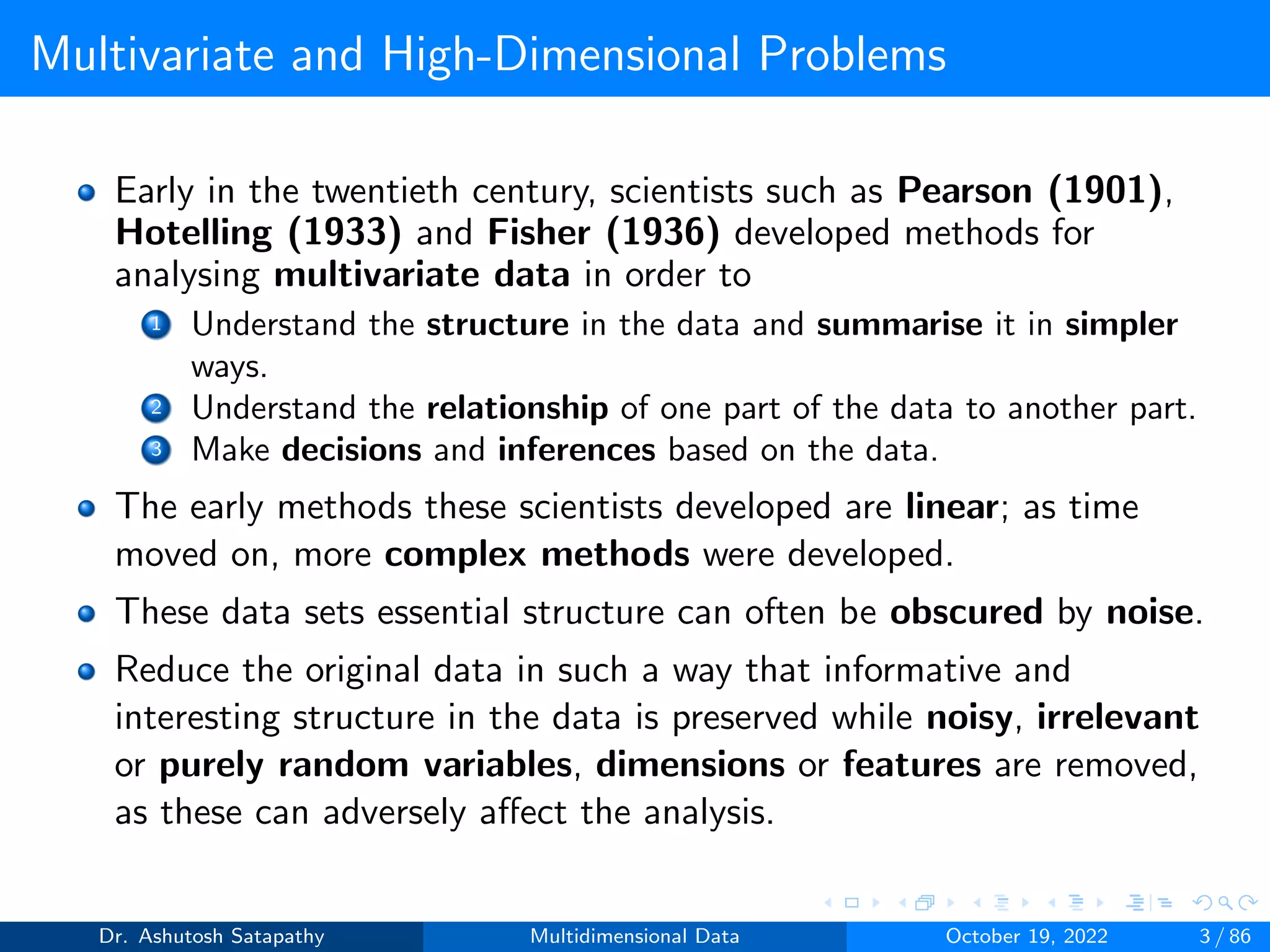
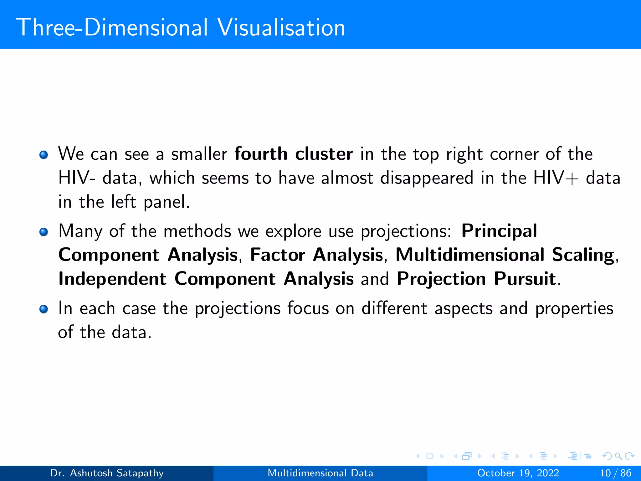
As the dimension grows, three-dimensional scatter-plots become
less relevant, unless we know that only some variables are important.
An alternative, which allows us to see all variables at once, present
the data in the form of parallel coordinate plots.
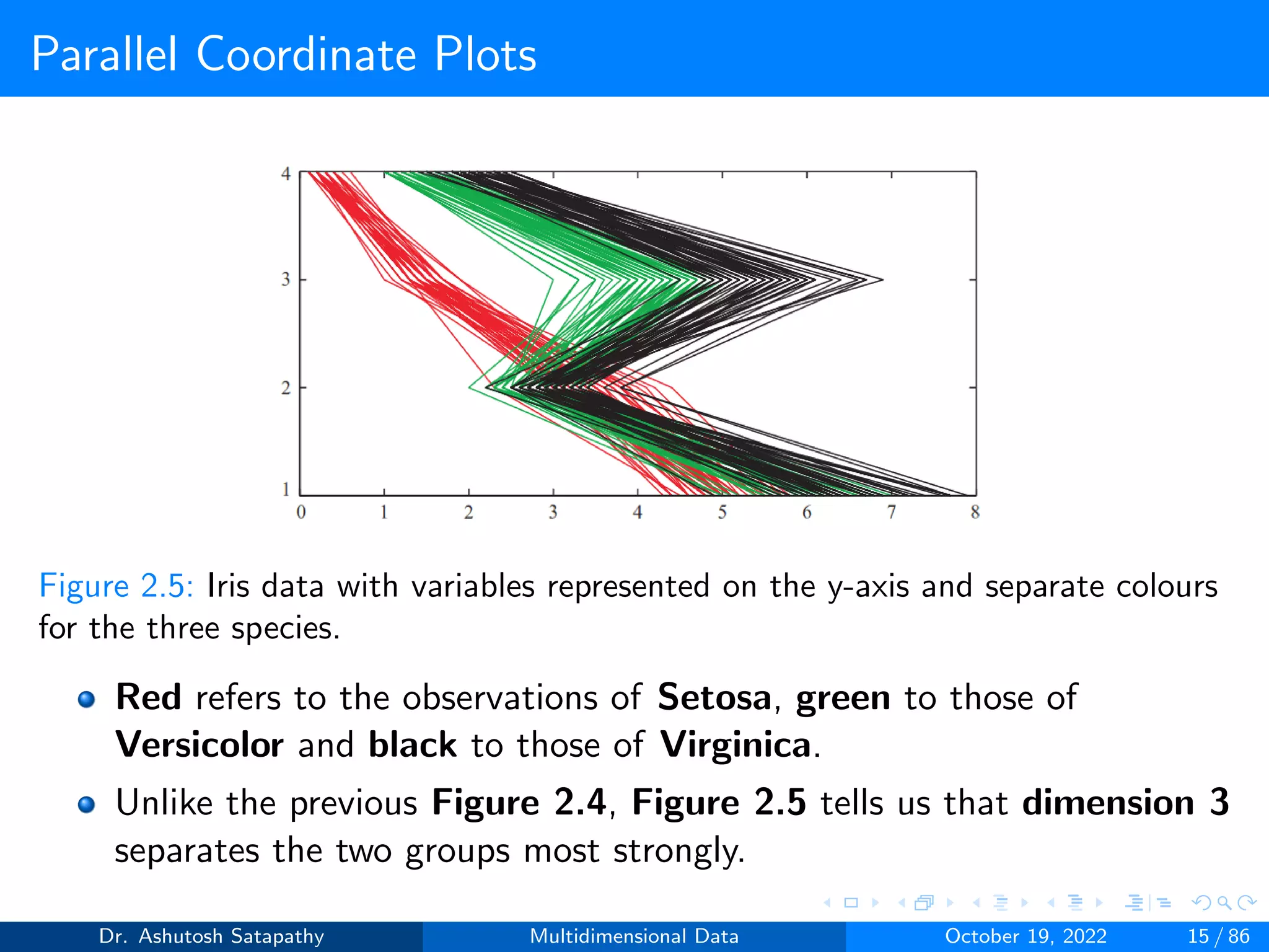
The idea is to present the data as two-dimensional graphs.
The variable numbers are represented as values on the y-axis in a
vertical parallel coordinate plot.
For a vector X = [X1,..., Xd ]T we represent the first variable X1 by
the point (X1, 1) and the jth variable Xj by (Xj , j).
Finally, we connect the d points by a line which goes from (X1, 1) to
(X2, 2) and so on to (Xd , d).
We apply the same rule to the next d-dimensional feature vectors.
Figure 2.5 shows a vertical parallel coordinate plot for Fisher’s iris
data.
Dr. Ashutosh Satapathy Multidimensional Data October 19, 2022 14 / 86](https://image.slidesharecdn.com/multidimensionaldata-221019141857-58826018/75/Multidimensional-Data-14-2048.jpg)
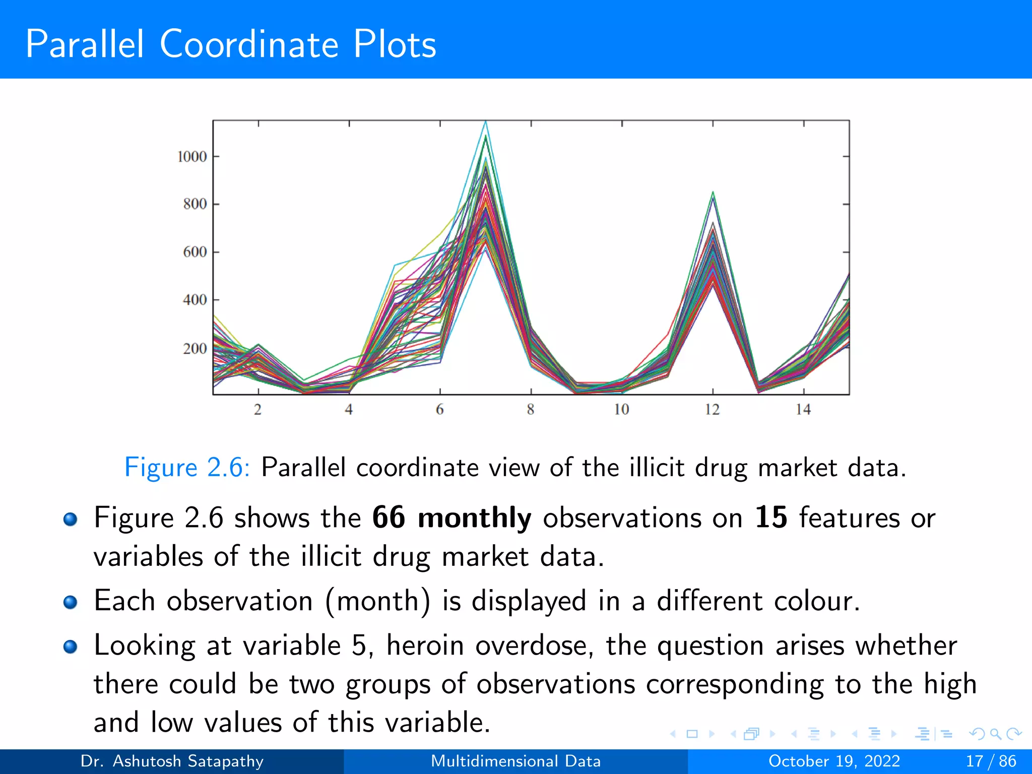
![Parallel Coordinate Plots
Instead of the three colours shown in Figure 2.5, different colors can
be used for each observation in Figure 2.6.
In a horizontal parallel coordinate plot, the x-axis represents the
variable numbers 1, ..., d. For a feature vector X = [X1 ··· Xd]T,
the first variable gives rise to the point (1, X1) and the jth variable
Xj to (j, Xj).
The d points are connected by a line, starting with (1, X1), then (2,
X2), until we reach (d, Xd).
As the variables are presented along the x-axis, horizontal parallel
coordinate plots are often used.
The differently coloured lines make it easier to trace particular
observations in Figure 2.6.
Dr. Ashutosh Satapathy Multidimensional Data October 19, 2022 16 / 86](https://image.slidesharecdn.com/multidimensionaldata-221019141857-58826018/75/Multidimensional-Data-16-2048.jpg)
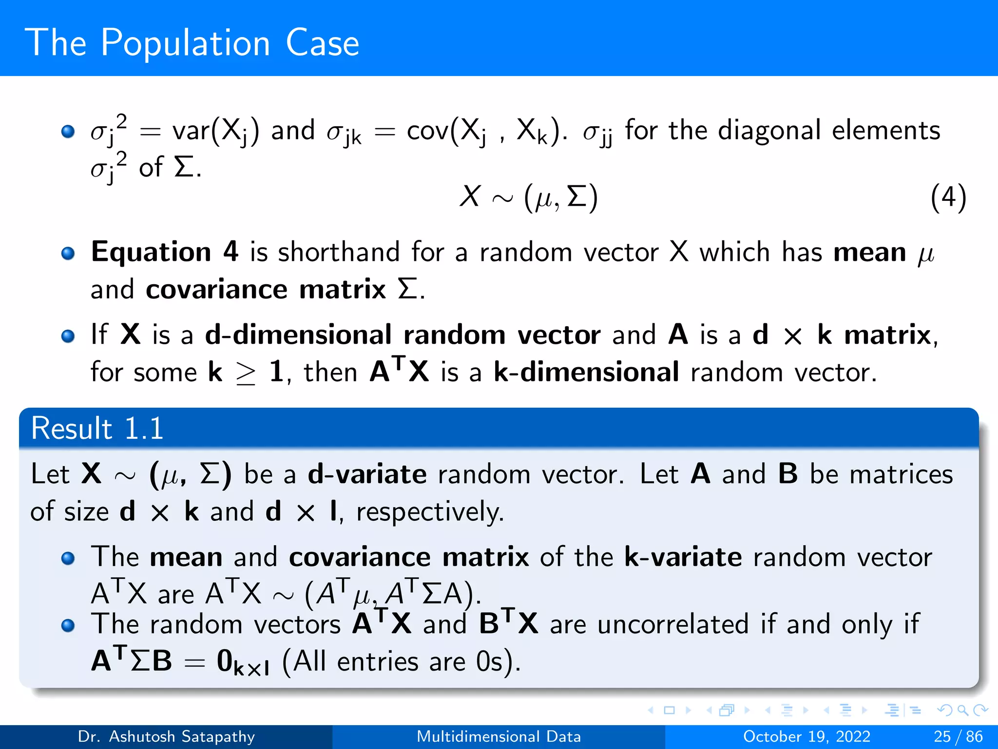
![The Population Case
Let X = [X1 X2... Xd ]T
(1)
be a random vector from a distribution F:Rd → [0, 1]. The individual
Xj, with j ≤ d are random variables, also called the variables,
components or entries of X. X is d-dimensional or d-variate.
X has a finite d-dimensional mean or expected value EX and a
finite d×d covariance matrix var(X).
µ = EX, Σ = var(X) = E[(X − µ)(X − µ)T
] (2)
The µ and Σ are
µ = [µ1 µ2... µd ]T
, Σ =
σ2
1 σ12 . . . σ1d
σ21 σ2
2 . . . σ2d
. . . . . .
. . . . . .
σd1 σd2 . . . σ2
d
(3)
Dr. Ashutosh Satapathy Multidimensional Data October 19, 2022 24 / 86](https://image.slidesharecdn.com/multidimensionaldata-221019141857-58826018/75/Multidimensional-Data-24-2048.jpg)
![The Population Case
Question 1: Suppose you have a set of n=5 data items, representing 5
insects, where each data item has a height (X), width (Y), and speed (Z)
(therefore d = 3)
Table 3.1: Three features of five different insects.
Height (cm) Width (cm) Speed (m/s)
I1 0.64 0.58 0.29
I2 0.66 0.57 0.33
I3 0.68 0.59 0.37
I4 0.69 0.66 0.46
I5 0.73 0.60 0.55
Solution:
mean (µ) = [0.64+0.66+0.68+0.69+0.73
5 , 0.58+0.57+0.59+0.66+0.60
5 ,
0.29+0.33+0.37+0.46+0.55
5 ]T = [0.68, 0.60, 0.40]T
Dr. Ashutosh Satapathy Multidimensional Data October 19, 2022 26 / 86](https://image.slidesharecdn.com/multidimensionaldata-221019141857-58826018/75/Multidimensional-Data-26-2048.jpg)
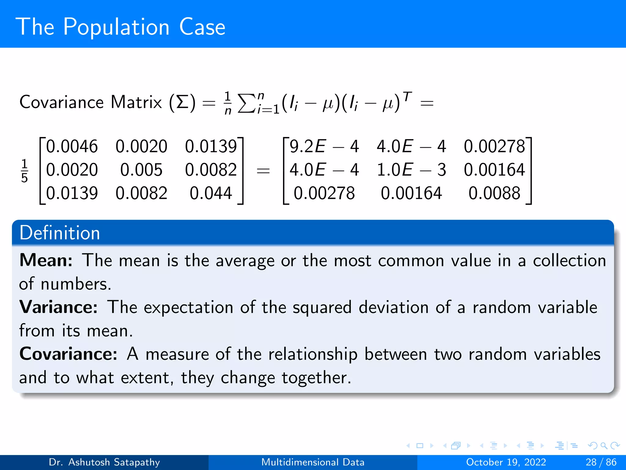
![The Population Case
I1-µ = [-0.04, -0.02, -0.11]T, (I1-µ)(I1-µ)T =
0.0016 0.0008 0.0044
0.0008 0.0004 0.0022
0.0044 0.0022 0.0121
I2-µ = [-0.02, -0.03, -0.07]T, (I2-µ)(I2-µ)T =
0.0004 0.0006 0.0014
0.0006 0.0009 0.0021
0.0014 0.0014 0.0049
I3-µ = [0, -0.01, -0.03]T, (I3-µ)(I3-µ)T =
0 0 0
0 0.0001 0.0003
0 0.0003 0.0009
I4-µ = [0.01, 0.06, 0.06]T, (I4-µ)(I4-µ)T =
0.0001 0.0006 0.0006
0.0006 0.0036 0.0036
0.0006 0.0036 0.0036
I5-µ = [0.05, 0, 0.15]T, (I5-µ)(I5-µ)T =
0.0025 0 0.0075
0 0 0
0.0075 0.0036 0.0225
Dr. Ashutosh Satapathy Multidimensional Data October 19, 2022 27 / 86](https://image.slidesharecdn.com/multidimensionaldata-221019141857-58826018/75/Multidimensional-Data-27-2048.jpg)
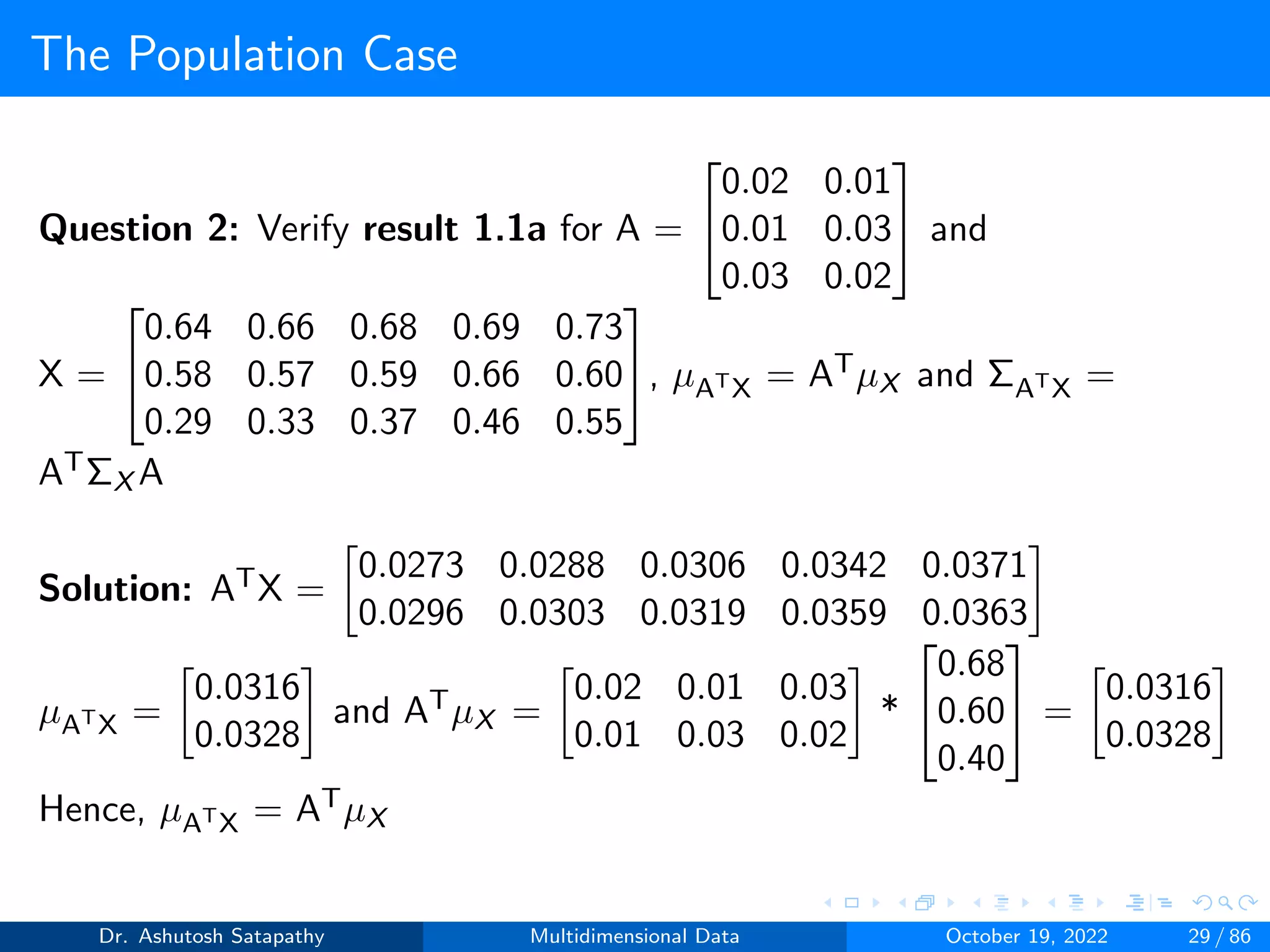
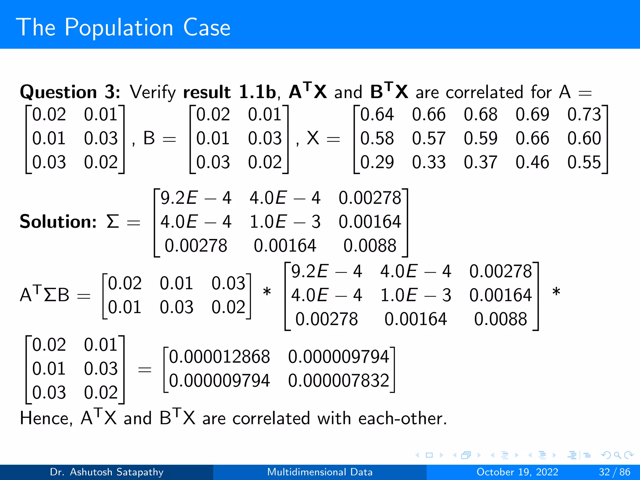
![The Population Case
ATΣX A =
0.02 0.01 0.03
0.01 0.03 0.02
*
9.2E − 4 4.0E − 4 0.00278
4.0E − 4 1.0E − 3 0.00164
0.00278 0.00164 0.0088
*
0.02 0.01
0.01 0.03
0.03 0.02
=
0.000012868 0.000009794
0.000009794 0.000007832
(ATX)1 - µATX = [-0.0043, -0.0032]T
((ATX)1 - µATX)((ATX)1 - µATX)T =
0.00001849 0.00001376
0.00001376 0.00001024
(ATX)2 - µATX = [-0.0028, -0.0025]T
((ATX)2 -µATX)((ATX)2 - µATX)T =
0.00000784 0.000007
0.000007 0.00000625
(ATX)3 - µATX = [-0.001, -0.0009]T
((ATX)3 -µATX)((ATX)3 - µATX)T =
0.000001 0.0000009
0.0000009 0.00000081
Dr. Ashutosh Satapathy Multidimensional Data October 19, 2022 30 / 86](https://image.slidesharecdn.com/multidimensionaldata-221019141857-58826018/75/Multidimensional-Data-30-2048.jpg)
![The Population Case
(ATX)4 - µATX = [0.0026, 0.0031]T
((ATX)4 -µATX)((ATX)4 - µATX)T =
0.00000676 0.00000806
0.00000806 0.00000961
(ATX)5 - µATX = [0.0055, 0.0035]T
((ATX)5 -µATX)((ATX)5 - µATX)T =
0.00003025 0.00001925
0.00001925 0.00001225
Covariance Matrix (ΣATX) = 1
n
Pn
i=1((ATX)i − µATX
)((ATX)i − µATX
)T
= 1
5
0.00006434 0.00004897
0.00004897 0.00003916
=
0.000012868 0.000009794
0.000009794 0.000007832
Hence ΣATX = ATΣX A
Dr. Ashutosh Satapathy Multidimensional Data October 19, 2022 31 / 86](https://image.slidesharecdn.com/multidimensionaldata-221019141857-58826018/75/Multidimensional-Data-31-2048.jpg)
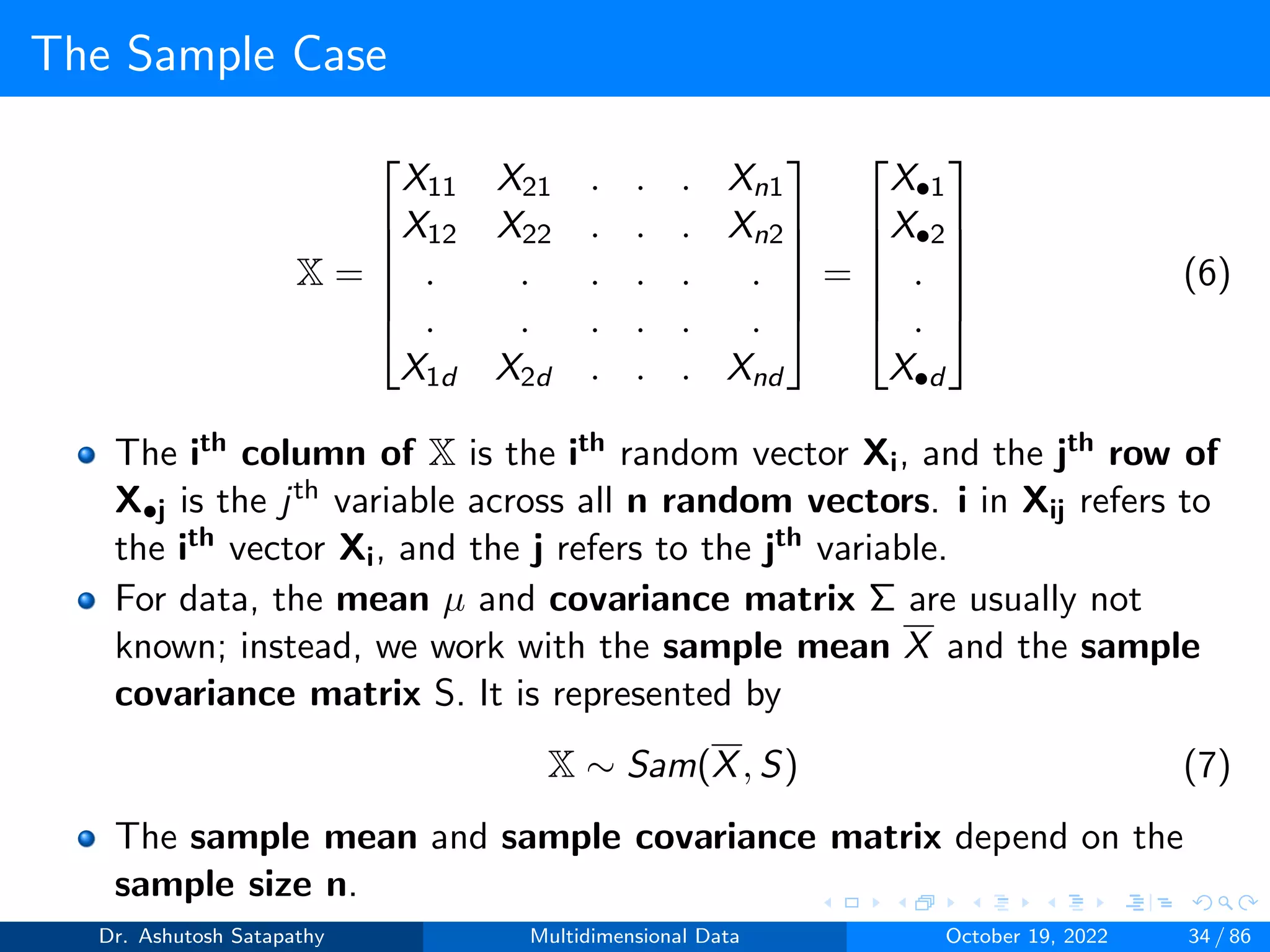
![The Sample Case
Let X1,...,Xn be d-dimensional random vectors. We assume that
the Xi are independent and from the same distribution F:Rd → [0,
1] with finite mean µ and covariance matrix Σ.
We omit reference to F when knowledge of the distribution is not
required, i.e., Rd → [0, 1].
In statistics one often identifies a random vector with its observed
values and writes Xi = xi
We explore properties of random samples but only encounter
observed values of random vectors. For this reason
X = [X1, X2, ..., Xn]T
(5)
for the sample of independent random vectors Xi and call this
collection a random sample or data.
Dr. Ashutosh Satapathy Multidimensional Data October 19, 2022 33 / 86](https://image.slidesharecdn.com/multidimensionaldata-221019141857-58826018/75/Multidimensional-Data-33-2048.jpg)
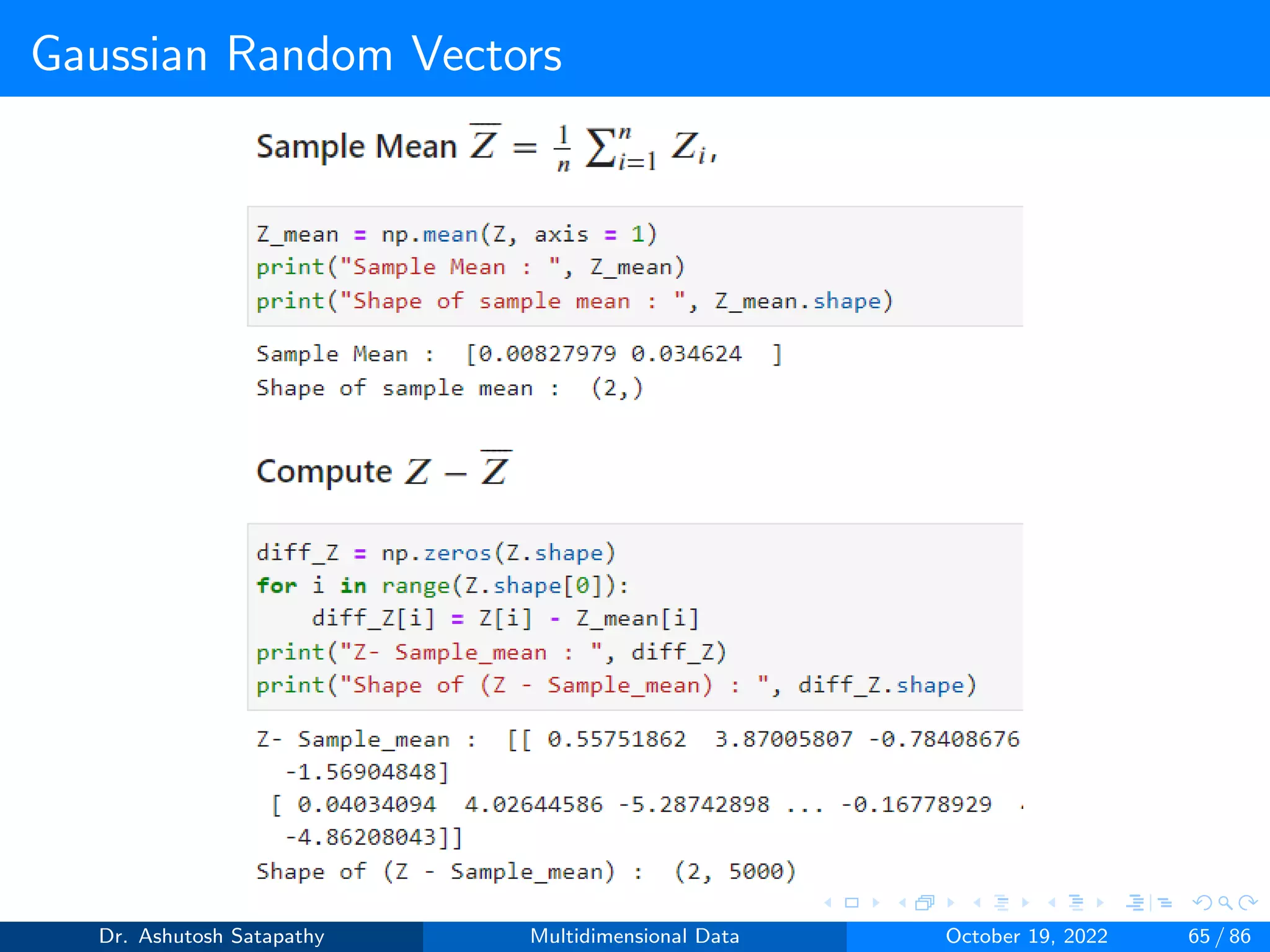
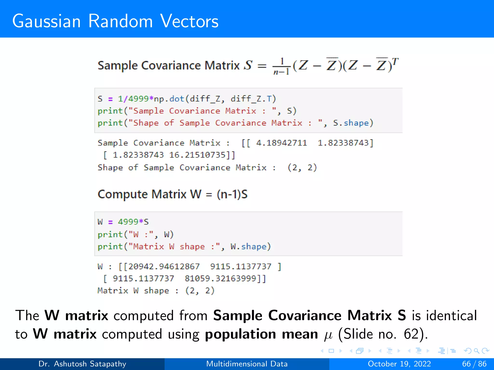
![The Sample Case
X =
1
n
n
X
i=1
Xi S =
1
n − 1
n
X
i=1
(Xi − X)(Xi − X)T
(8)
Definitions of the sample covariance matrix use n-1 or (n-1)-1 in
the literature. (n-1)-1 is preferred as an unbiased estimator of the
population variance Σ.
Xcent = X − X = [X1 − X, X2 − X, ..., Xn − X] (9)
Xcent is the centred data and it is of size dxn. Using this notation,
the d×d sample covariance matrix S becomes
S =
1
n − 1
XcentXT
cent =
1
n − 1
(X − X)(X − X)T
(10)
Dr. Ashutosh Satapathy Multidimensional Data October 19, 2022 35 / 86](https://image.slidesharecdn.com/multidimensionaldata-221019141857-58826018/75/Multidimensional-Data-35-2048.jpg)
![The Sample Case
The entries of the sample covariance matrix S are sjk, and
sjk =
1
n − 1
n
X
i=1
(Xij − mj )(Xik − mk) (11)
X =[m1,...,md]T, and mj is the sample mean of the jth variable.
As for the population, we write sj
2 or sjj for the diagonal elements
of S.
Consider a ∈ Rd; then the projection of X onto a is aTX.
Similarly, the projection of the matrix X onto a is done element-wise
for each random vector Xi and results in the 1×n vector aTX.
Dr. Ashutosh Satapathy Multidimensional Data October 19, 2022 36 / 86](https://image.slidesharecdn.com/multidimensionaldata-221019141857-58826018/75/Multidimensional-Data-36-2048.jpg)
![The Sample Case
Question 4: The math and science scores of good, average and poor
students from a class are given as follows:
Student Math (X) Science (Y)
1 92 68
2 55 30
3 100 78
Find the sample mean (X), covariance matrix (S), S12 of the above data.
Solution: X =
92 55 100
68 30 78
X =
92+55+100
3
68+30+78
3
=
82.33
58.66
X1 − X = [9.67, 9.34]T , (X1 − X)(X1 − X)T =
93.5089 90.3178
90.3178 87.2356
X2 − X = [−27.33, −28.66]T
(X2 − X)(X2 − X)T =
746.9289 783.2778
783.2778 821.3956
Dr. Ashutosh Satapathy Multidimensional Data October 19, 2022 37 / 86](https://image.slidesharecdn.com/multidimensionaldata-221019141857-58826018/75/Multidimensional-Data-37-2048.jpg)
![The Sample Case
X3 − X = [17.67, 19.34]T , (X3 − X)(X3 − X)T =
312.2289 341.7378
341.7378 374.0356
Sample covariance matrix (S) = 1
n−1
Pn
i=1(Xi − X)(Xi − X)T =
1
2
1152.6667 1215.3334
1215.3334 1282.6668
=
576.3335 607.6667
607.6667 641.3334
From Equation 11, S12 = 1
2
P3
i=1(Xi1 − m1)(Xi2 − m2)
S12 = 1
2[(X11 −m1)(X12 −m2)+(X21 −m1)(X22 −m2)+(X31 −m1)(X32−
m2)] = 1
2[(92 − 82.33)(68 − 58.66) + (55 − 82.33)(30 − 58.66) + (100 −
82.33)(78 − 58.66)] = 607.6667
Dr. Ashutosh Satapathy Multidimensional Data October 19, 2022 38 / 86](https://image.slidesharecdn.com/multidimensionaldata-221019141857-58826018/75/Multidimensional-Data-38-2048.jpg)
![The Sample Case
Question 5: Compute projection of matrix X =
92 55 100
68 30 78
onto a
vector
−45
45
.
Solution: P = aTX =
−45 45
*
92 55 100
68 30 78
=
−1080 −1125 −990
So, projection of X onto a vector [−45, 45]T is a 1x3 matrix.
Dr. Ashutosh Satapathy Multidimensional Data October 19, 2022 39 / 86](https://image.slidesharecdn.com/multidimensionaldata-221019141857-58826018/75/Multidimensional-Data-39-2048.jpg)
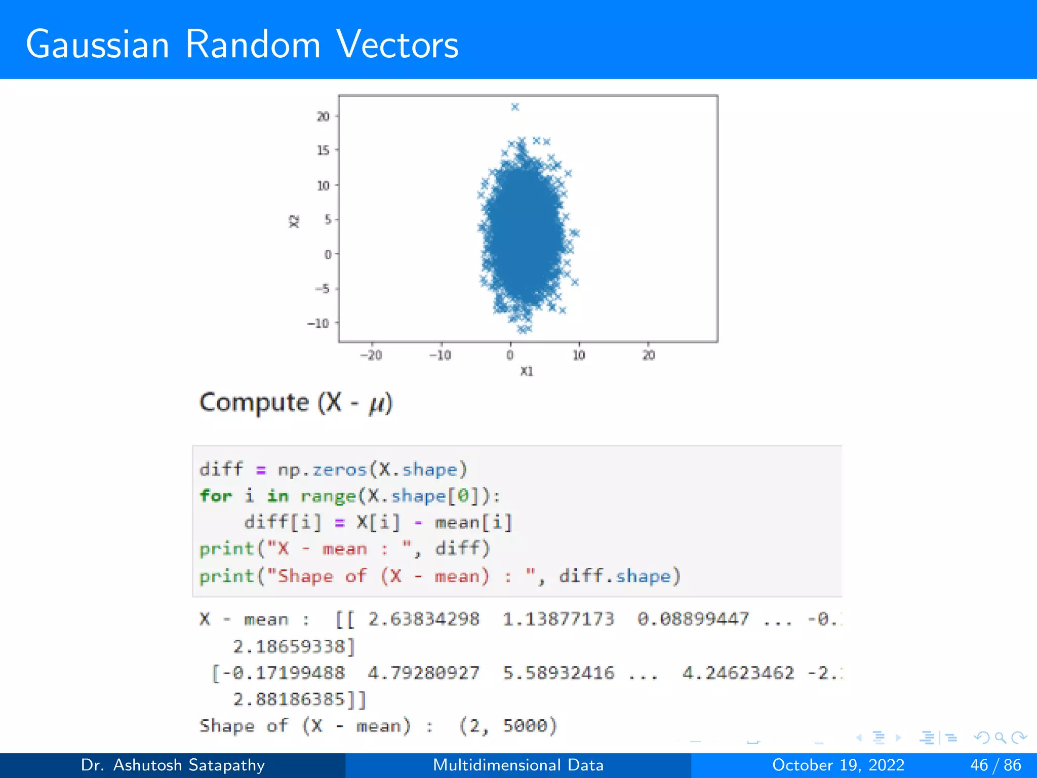
![Gaussian Random Vectors
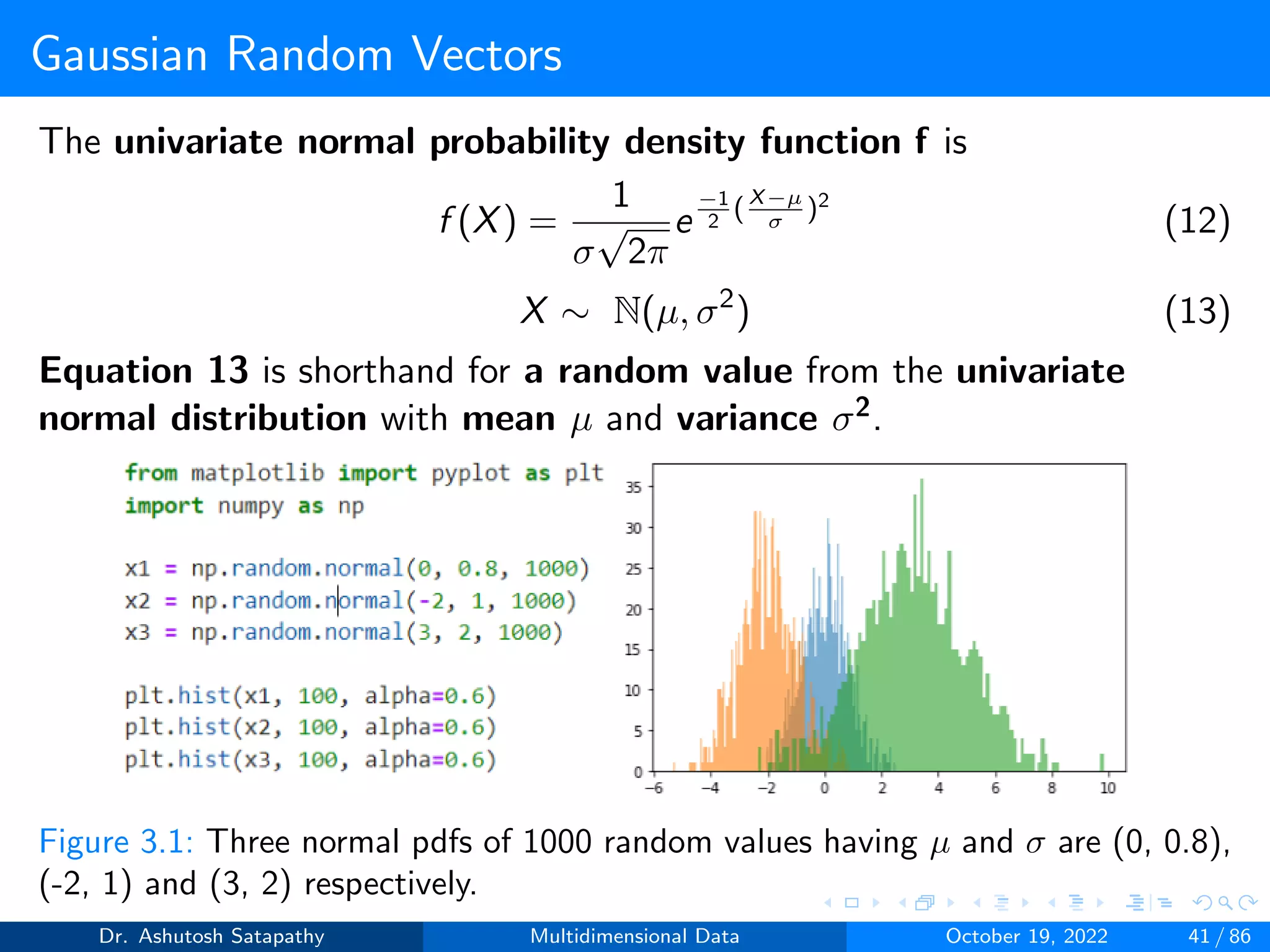
The d-variate normal probability density function f is
f (X) = (2π)−d
2 |Σ|−1
2 exp
−1
2(X − µ)T Σ−1(X − µ)
(14)
X ∼ N(µ, Σ) (15)
Equation 15 is shorthand for a d-dimensional random vector from the
d-variate normal distribution with mean µ and covariance matrix Σ.
Figure 3.2: 2-dimensional normal pdf having µ = [1, 2] and Σ =
0.25 0.3
0.3 1
Dr. Ashutosh Satapathy Multidimensional Data October 19, 2022 42 / 86](https://image.slidesharecdn.com/multidimensionaldata-221019141857-58826018/75/Multidimensional-Data-42-2048.jpg)
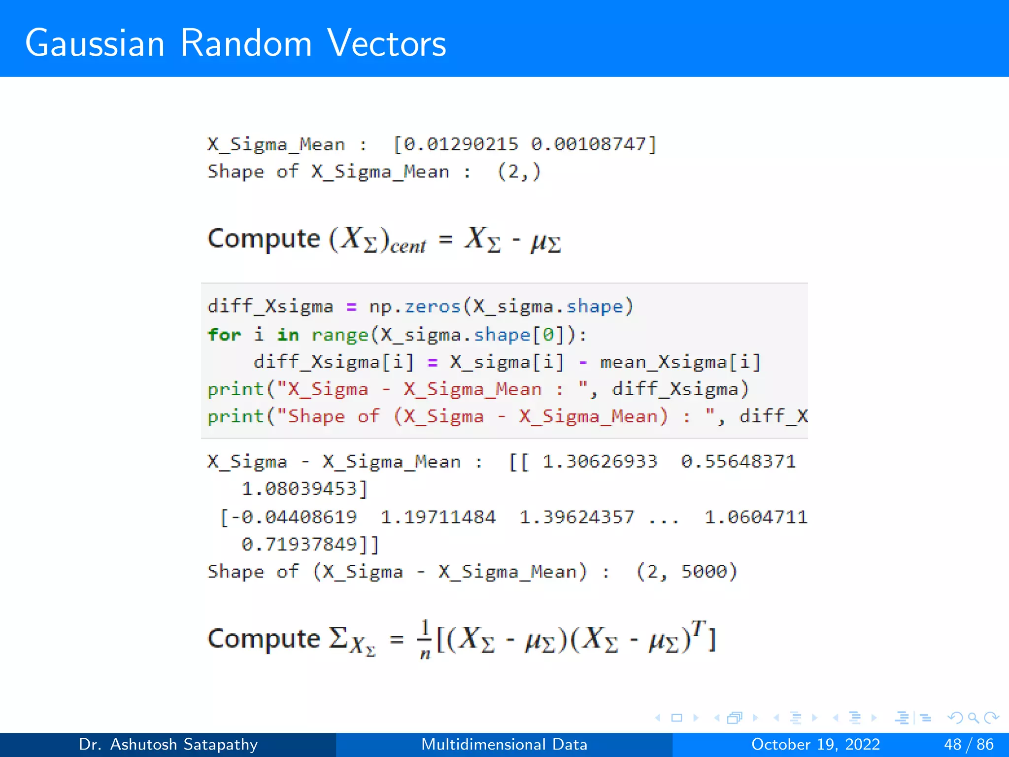
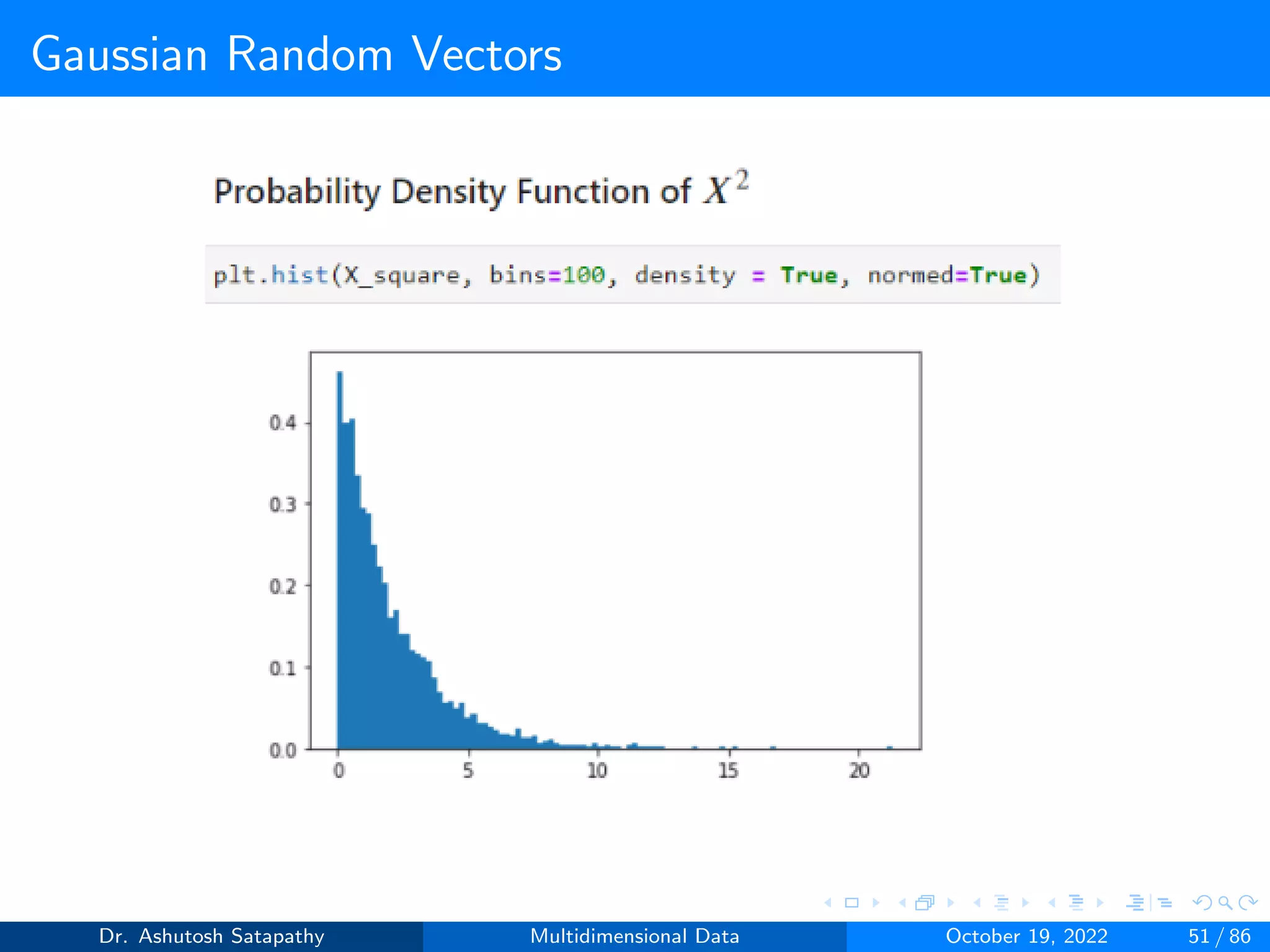
![Gaussian Random Vectors
Result 1.2
Let X ∼ N(µ, Σ) be d-variate, and assume that Σ−1 exists.
1 Let XΣ = Σ−1/2(X − µ); then XΣ ∼ N(0, Id×d), where Id×d is the
d×d identity matrix.
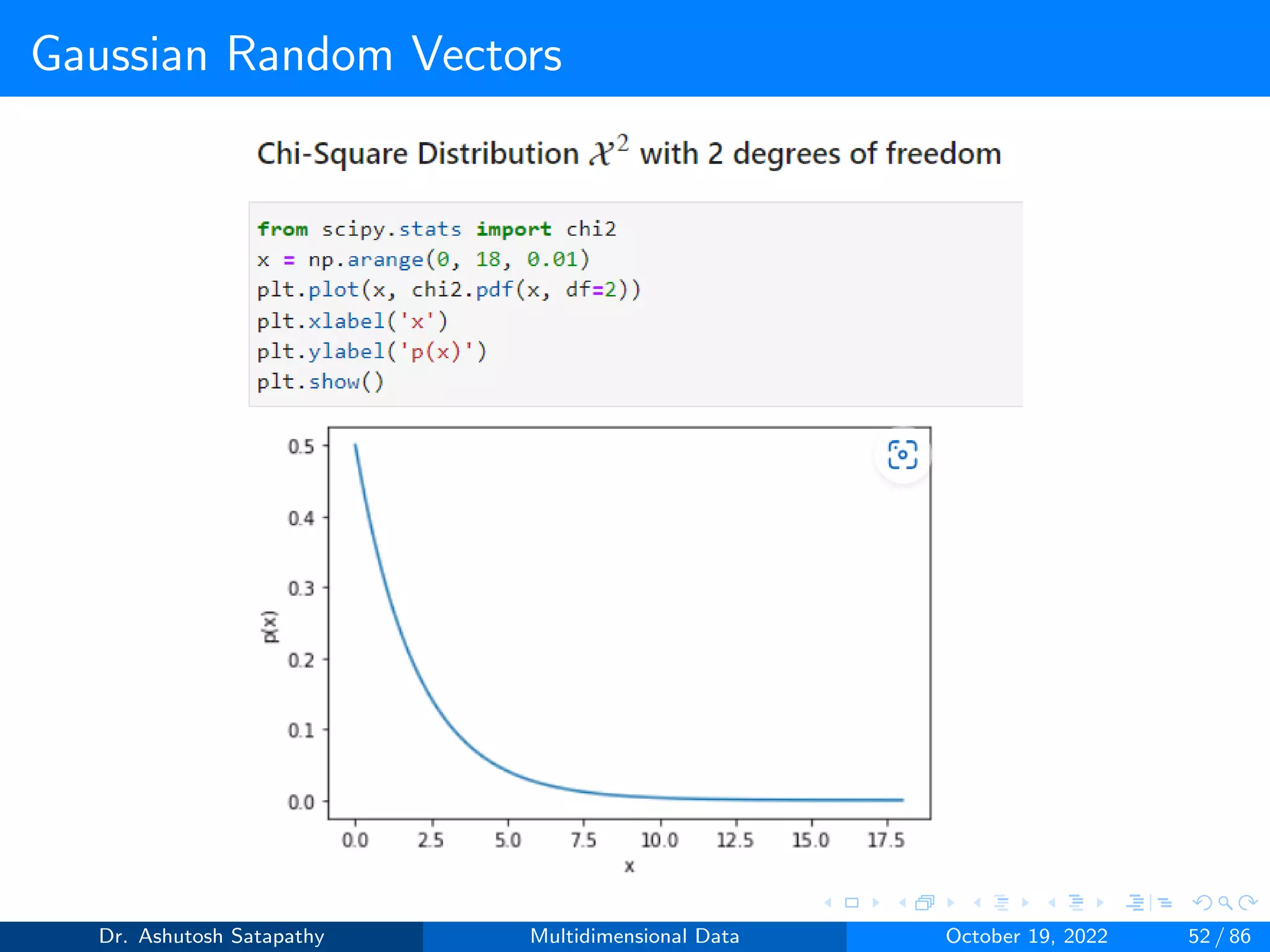
2 Let X2 = (X-µ)TΣ-1(X-µ); then X2 ∼ Xd
2, the Chi-squared X2
distribution in d degrees of freedom.
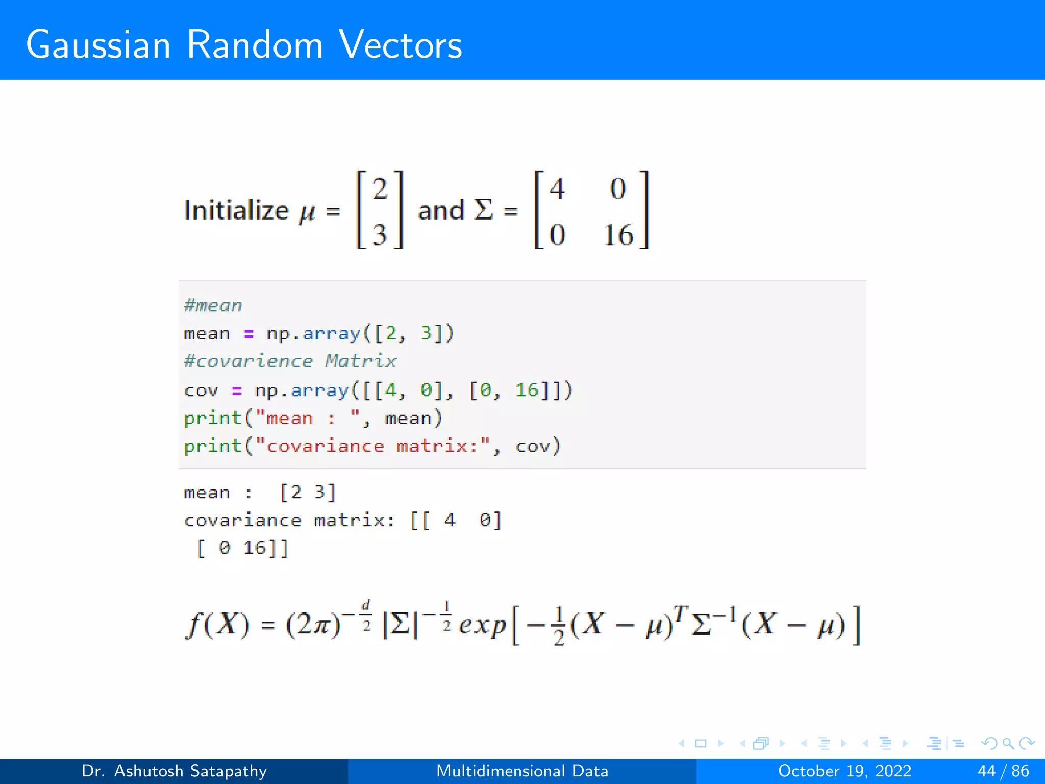
Question 6: Let X ∼ N(µ, Σ) be 2-variate, where µ = [2, 3]T , Σ =
4 0
0 16
and Σ−1 =
0.25 0
0 0.0625
. Verify Result 1.2.1 and 1.2.2
Solution:
Dr. Ashutosh Satapathy Multidimensional Data October 19, 2022 43 / 86](https://image.slidesharecdn.com/multidimensionaldata-221019141857-58826018/75/Multidimensional-Data-43-2048.jpg)

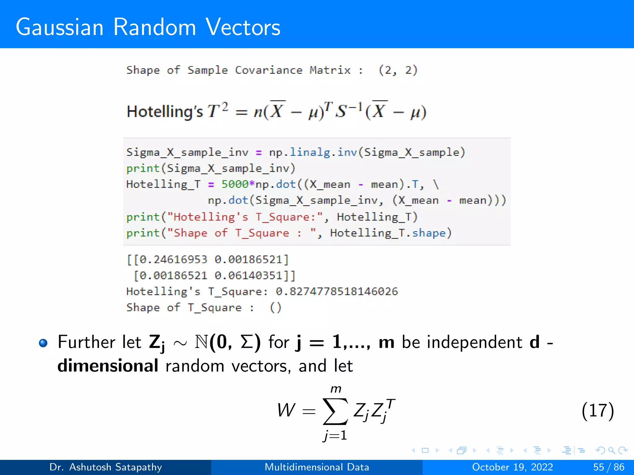
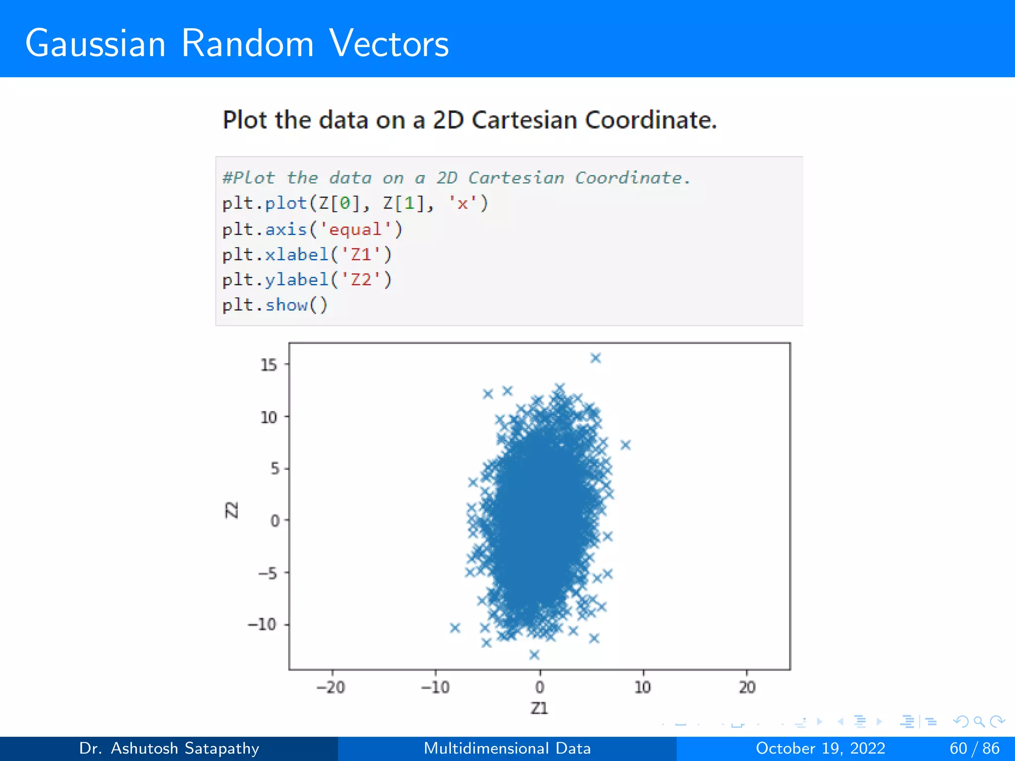
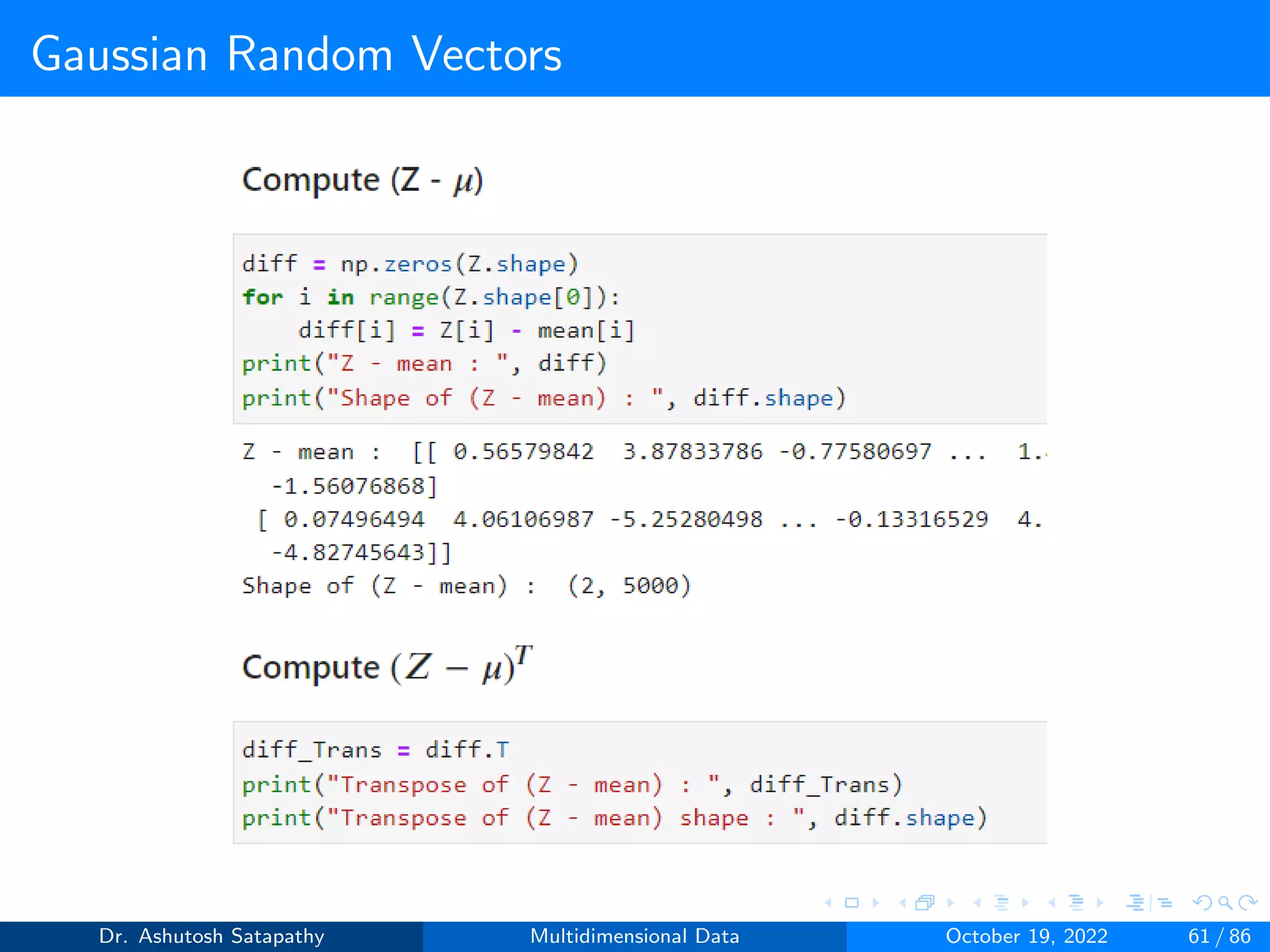
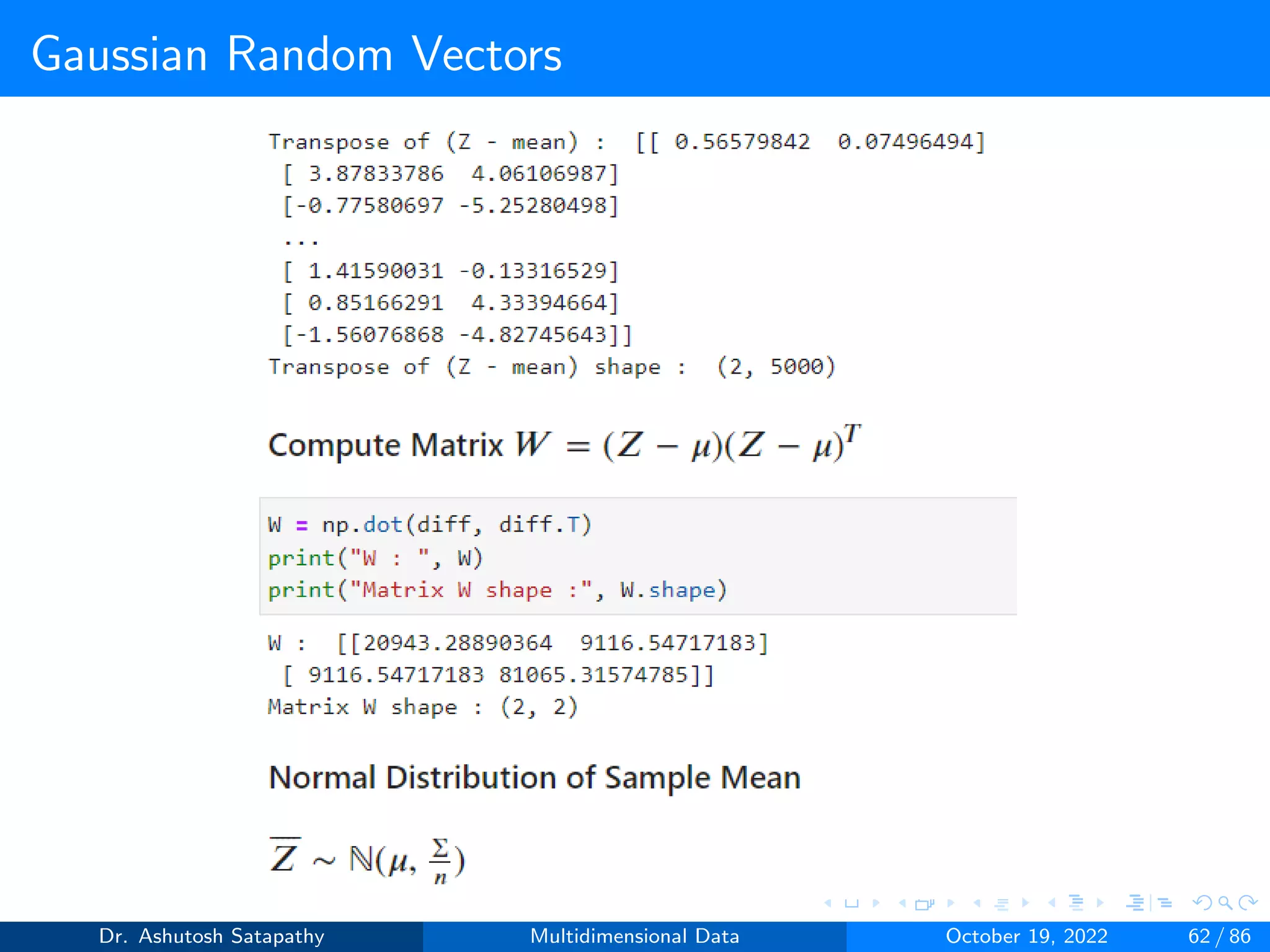
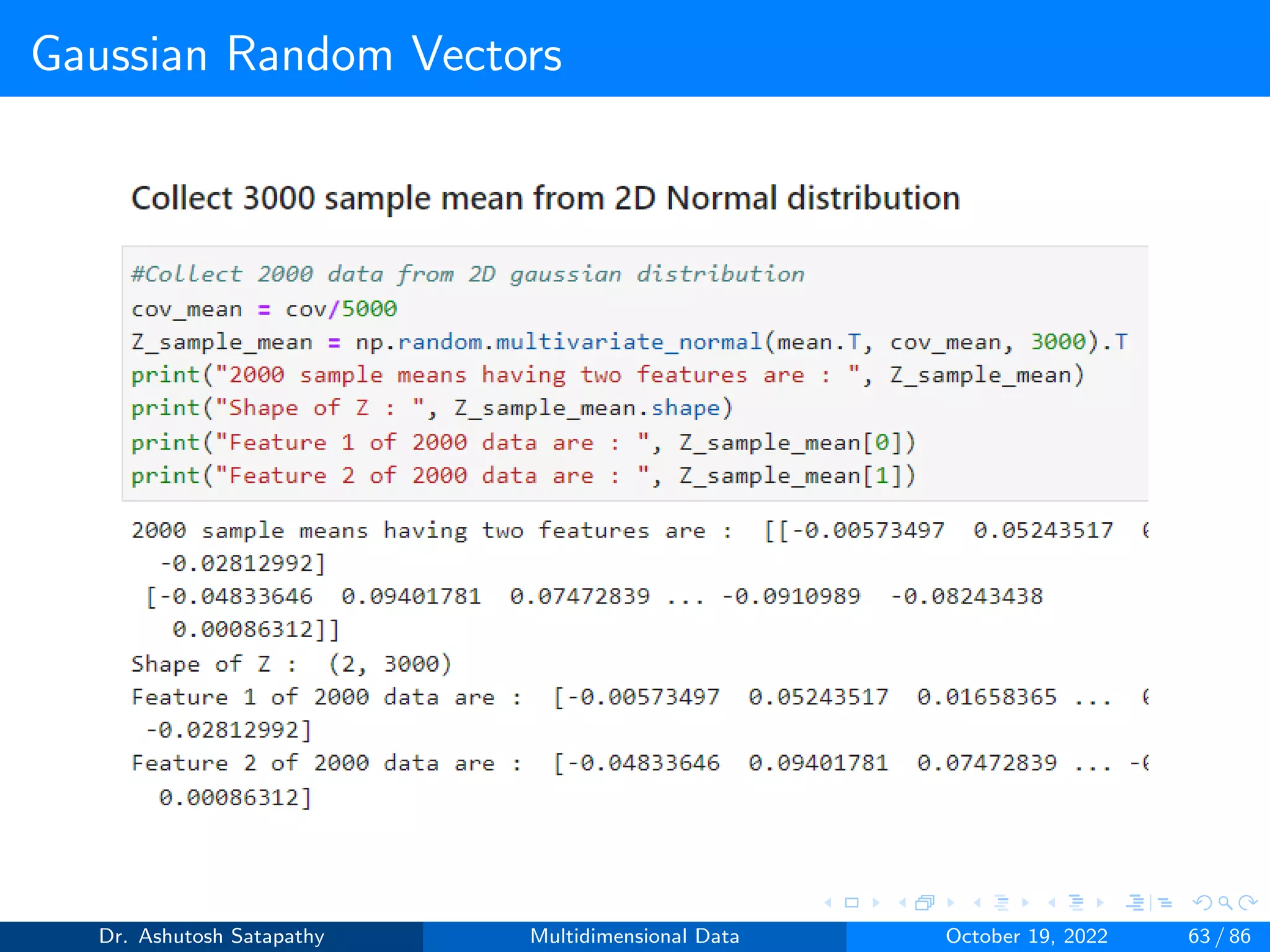
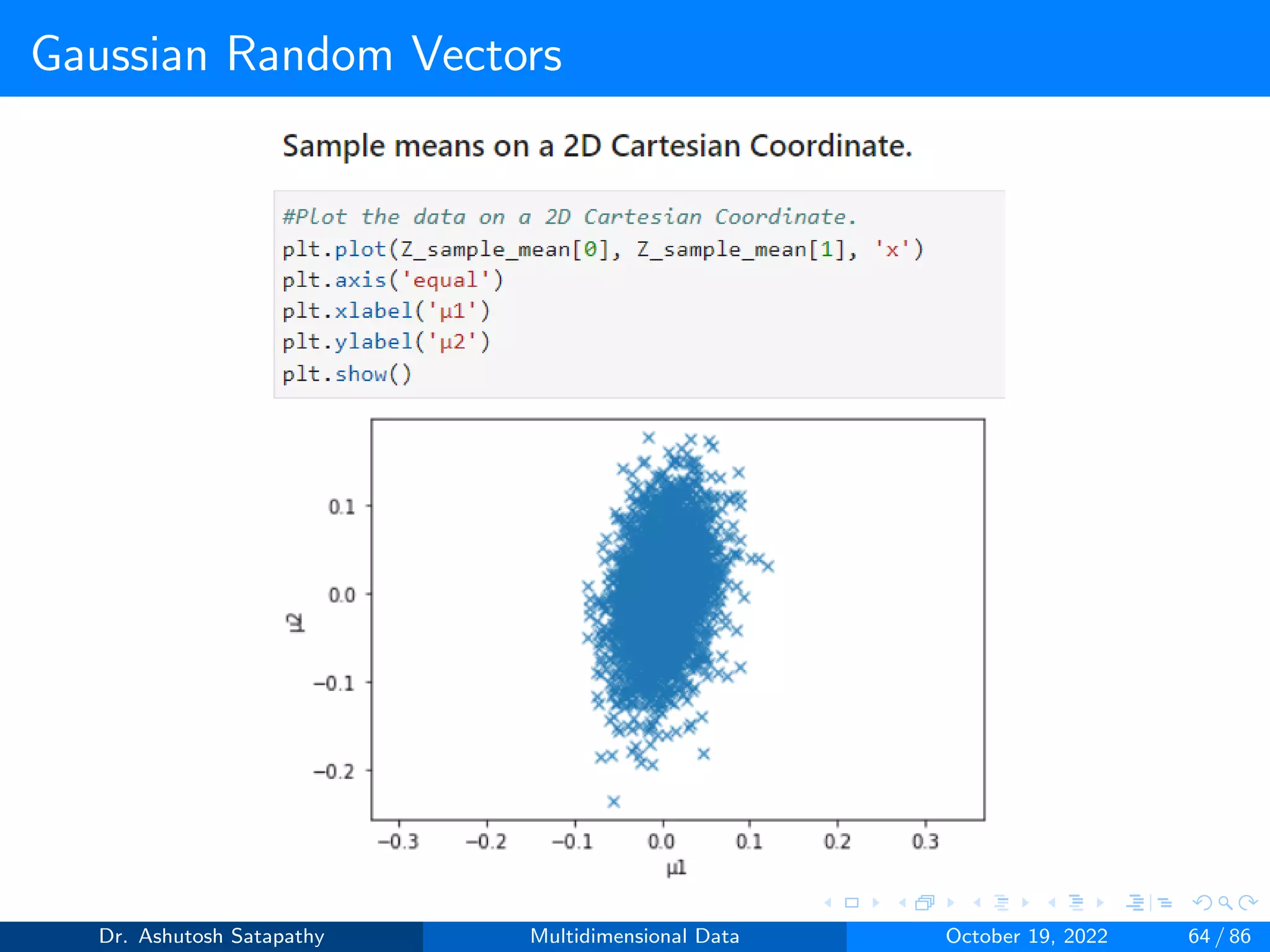
![Gaussian Random Vectors
Question 8: Let Z ∼ N(µ, Σ) 2-variate, where µ = [0, 0]T , Σ =
4 2
2 16
.
Compute W and (n-1)S matrices, and plot sample mean distribution.
Dr. Ashutosh Satapathy Multidimensional Data October 19, 2022 58 / 86](https://image.slidesharecdn.com/multidimensionaldata-221019141857-58826018/75/Multidimensional-Data-58-2048.jpg)
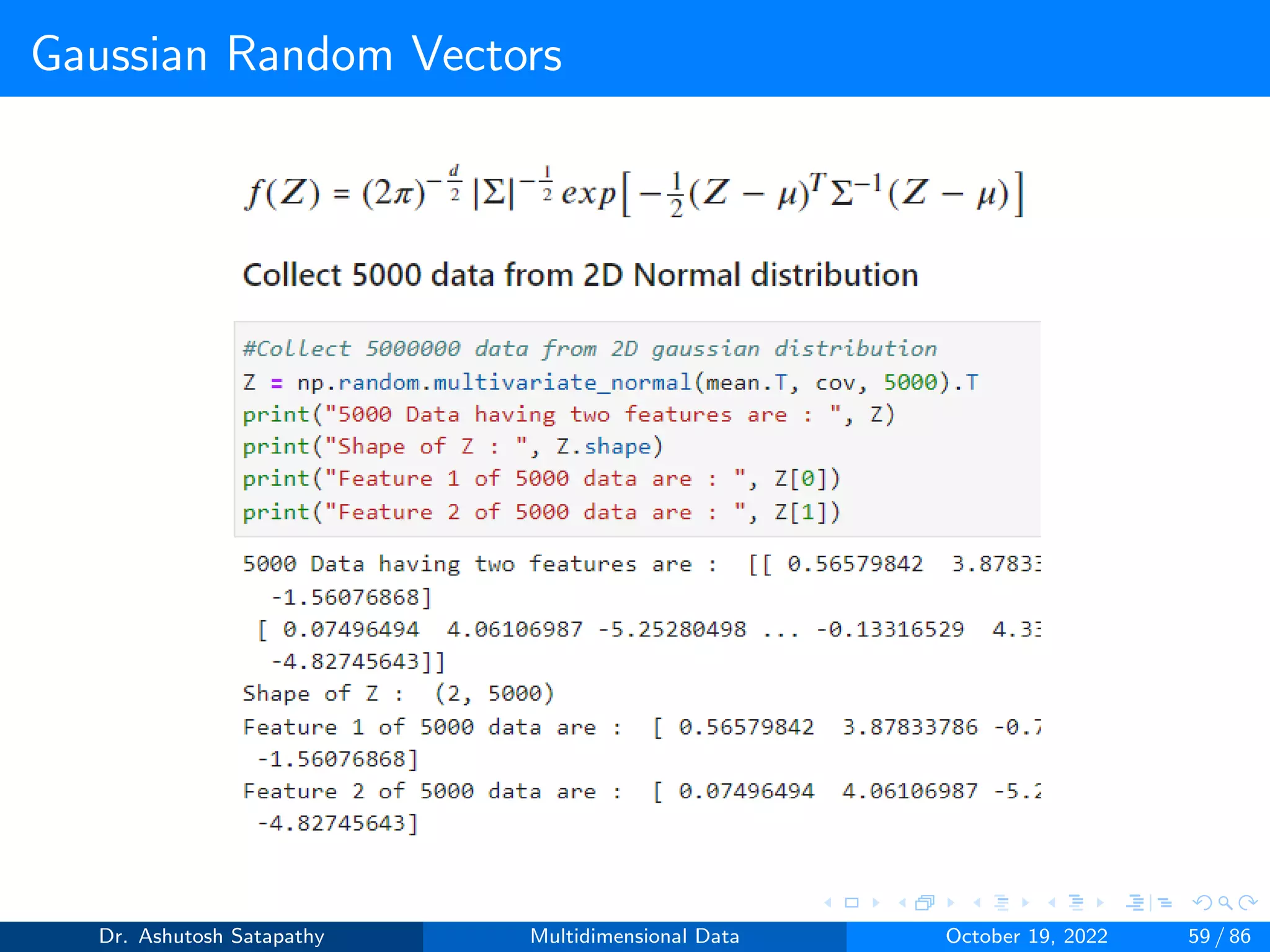
![Gaussian Random Vectors
Let X ∼ (µ, Σ) be d-dimensional. The multivariate normal
probability density function f is
f (Xi ) = (2π)−d
2 det(Σ)−1
2 exp
−1
2(Xi − µ)T Σ−1(Xi − µ)
(19)
Where det(σ) is the determinant of Σ and X = [X1, X2, ···, Xn] of
independent random vectors from the normal distribution with
the mean µ and covariance matrix Σ.
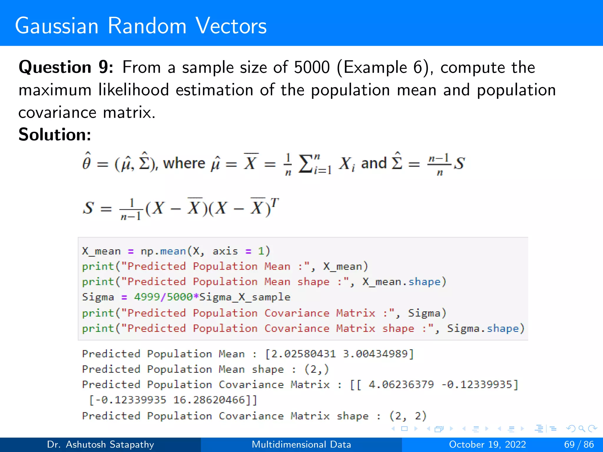
The normal or Gaussian likelihood (function) L as a function of
the parameter θ of interest conditional on the data.
L(θ|X) = (2π)−nd
2 det(Σ)−n
2 exp
−1
2(Xi − µ)T Σ−1(Xi − µ)
(20)
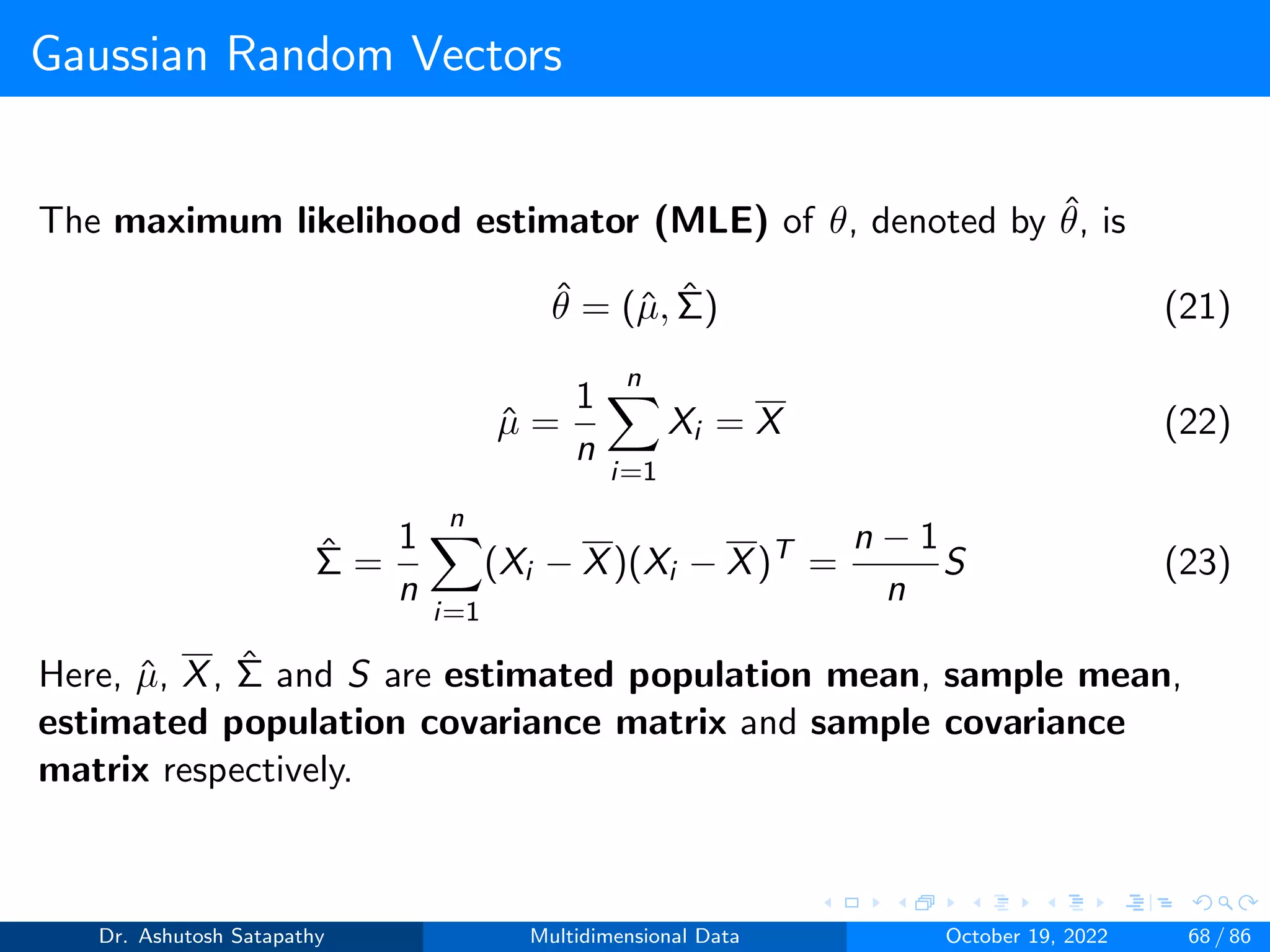
The parameter of interest θ is mean µ and the covariance matrix
Σ. So, θ = (µ, Σ).
Dr. Ashutosh Satapathy Multidimensional Data October 19, 2022 67 / 86](https://image.slidesharecdn.com/multidimensionaldata-221019141857-58826018/75/Multidimensional-Data-67-2048.jpg)
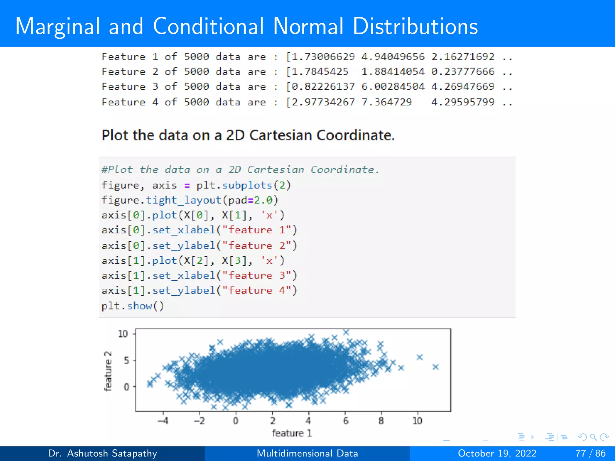
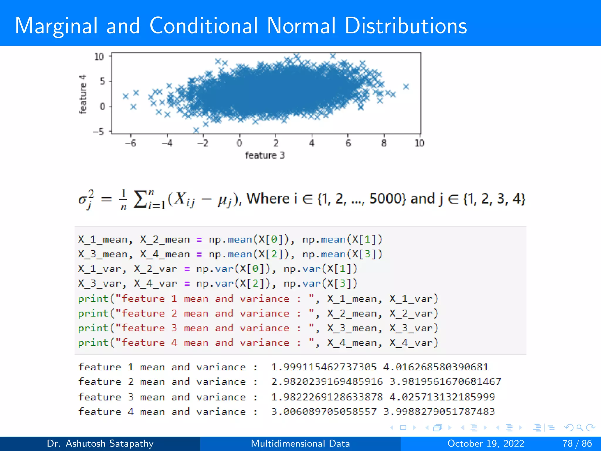
![Marginal and Conditional Normal Distributions
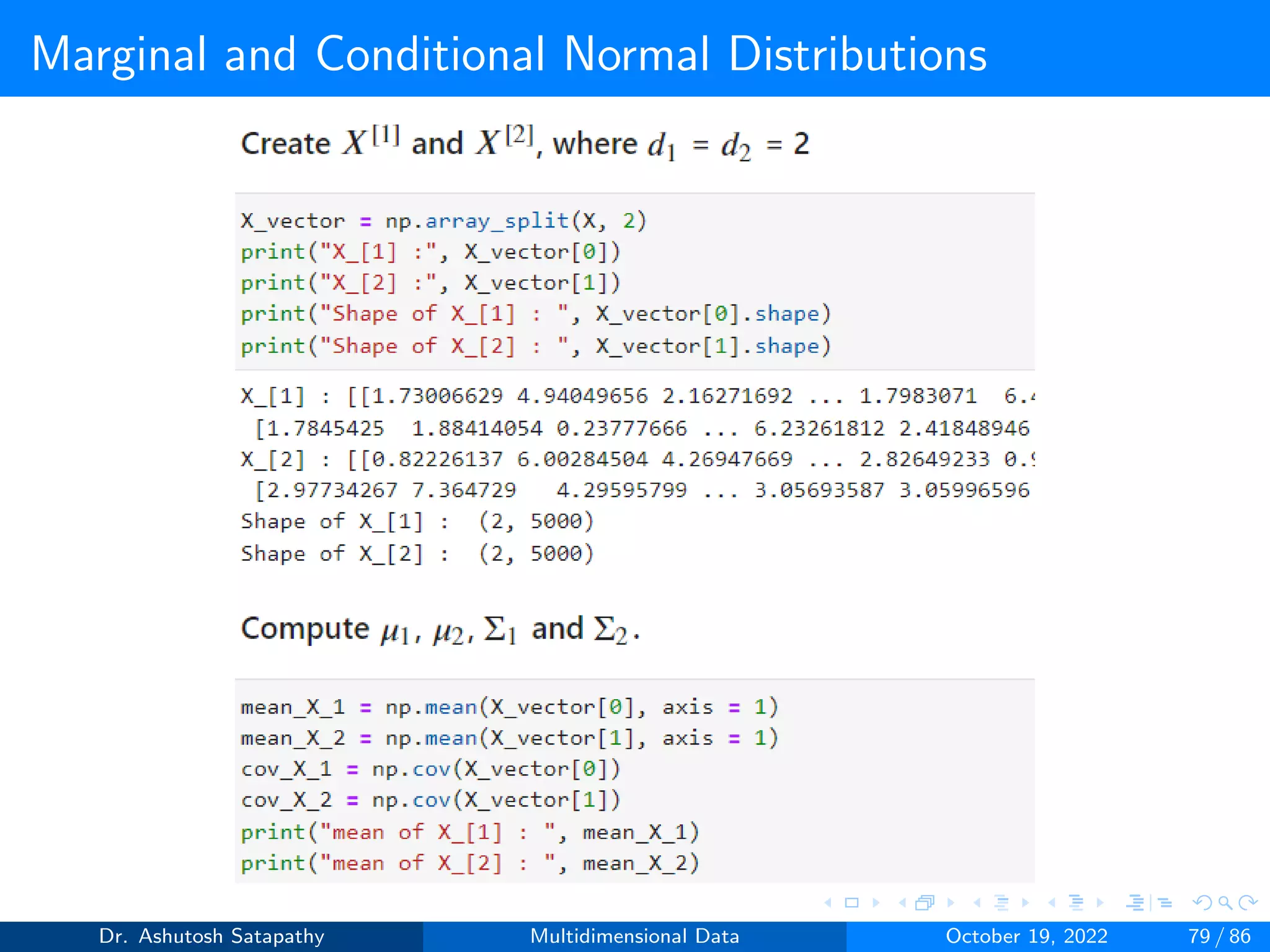
Consider a normal random vector X = [X1, X2,..., Xd]T. Let X[1] be a
vector consisting of the first d1 entries of X, and let X[2] be the vector
consisting of the remaining d2 entries:
X =
X[1]
X[2]
(24)
For ι = 1, 2 we let µι be the mean of X[ι] and Σι its covariance matrix.
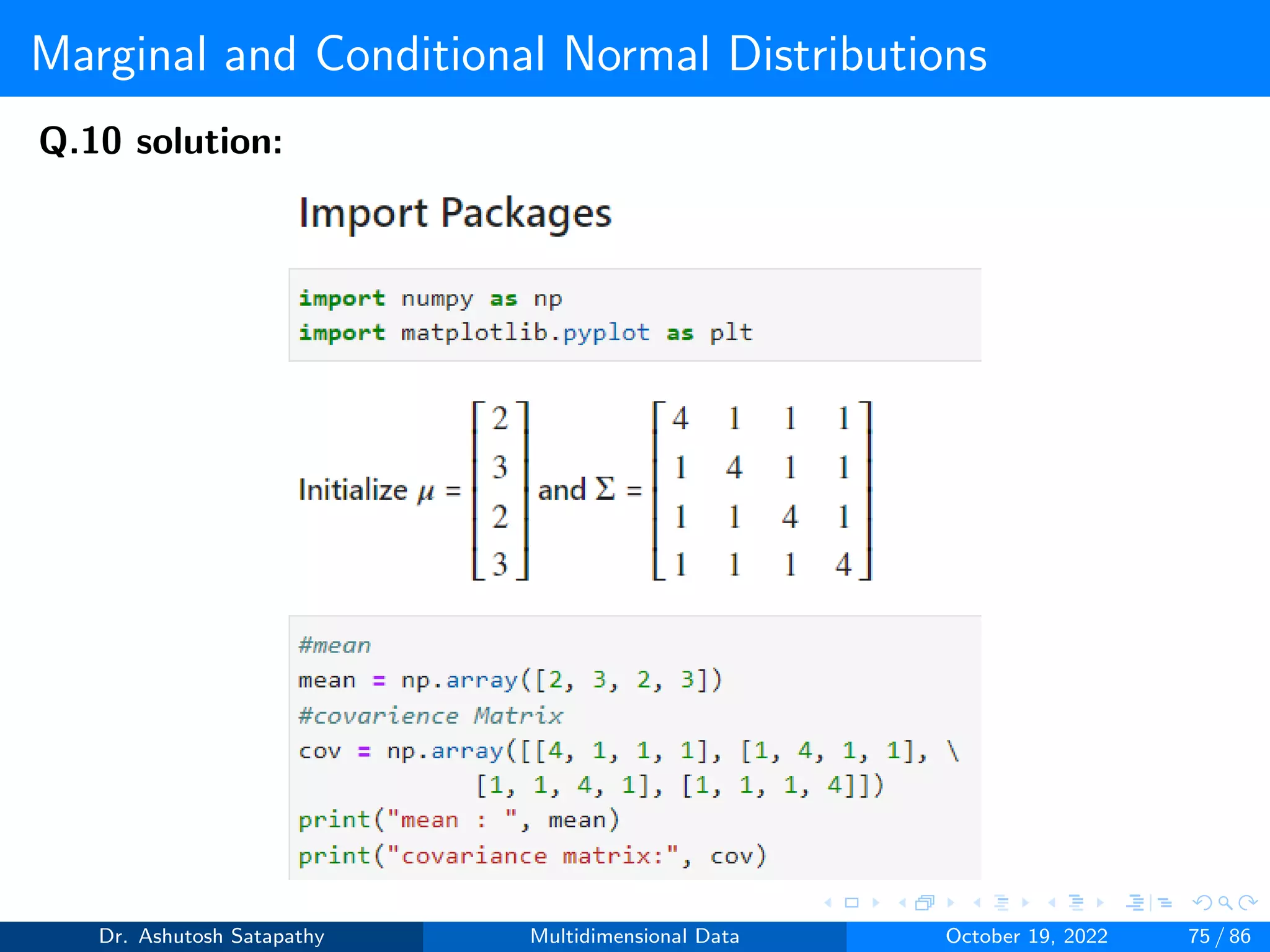
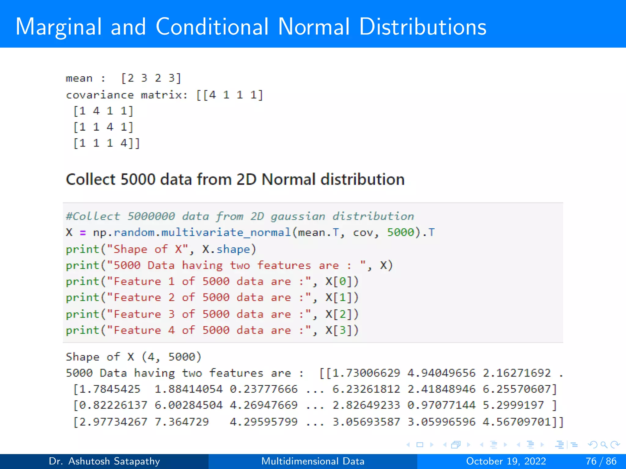
Question 10: Let X ∼ N(µ, Σ) be 4-variate, where µ = [2, 3, 2, 3]T ,
Σ =
4 1 1 1
1 4 1 1
1 1 4 1
1 1 1 4
Σ−1 =
0.286 −0.048 −0.048 −0.048
−0.048 0.286 −0.048 −0.048
−0.048 −0.048 0.286 −0.048
−0.048 −0.048 −0.048 0.286
.
Compute µ1 and Σ1 of X[1] and µ2 and Σ2 of X[2], where d1 and d2 are 2.
Analyze all the properties from Result 1.4 and 1.5.
Dr. Ashutosh Satapathy Multidimensional Data October 19, 2022 71 / 86](https://image.slidesharecdn.com/multidimensionaldata-221019141857-58826018/75/Multidimensional-Data-71-2048.jpg)
![Marginal and Conditional Normal Distributions
Result 1.4
Assume that X[1], X[2] and X are given by Equation 24 for some d1, d2
d such that d1 + d2 = d. Assume also that X ∼ N(µ, Σ).
1 For j = 1,...,d the jth variable Xj of X has the distribution N(µj , σ2
j ).
2 ι = 1, 2, X[ι] has the distribution N(µι, Σι).
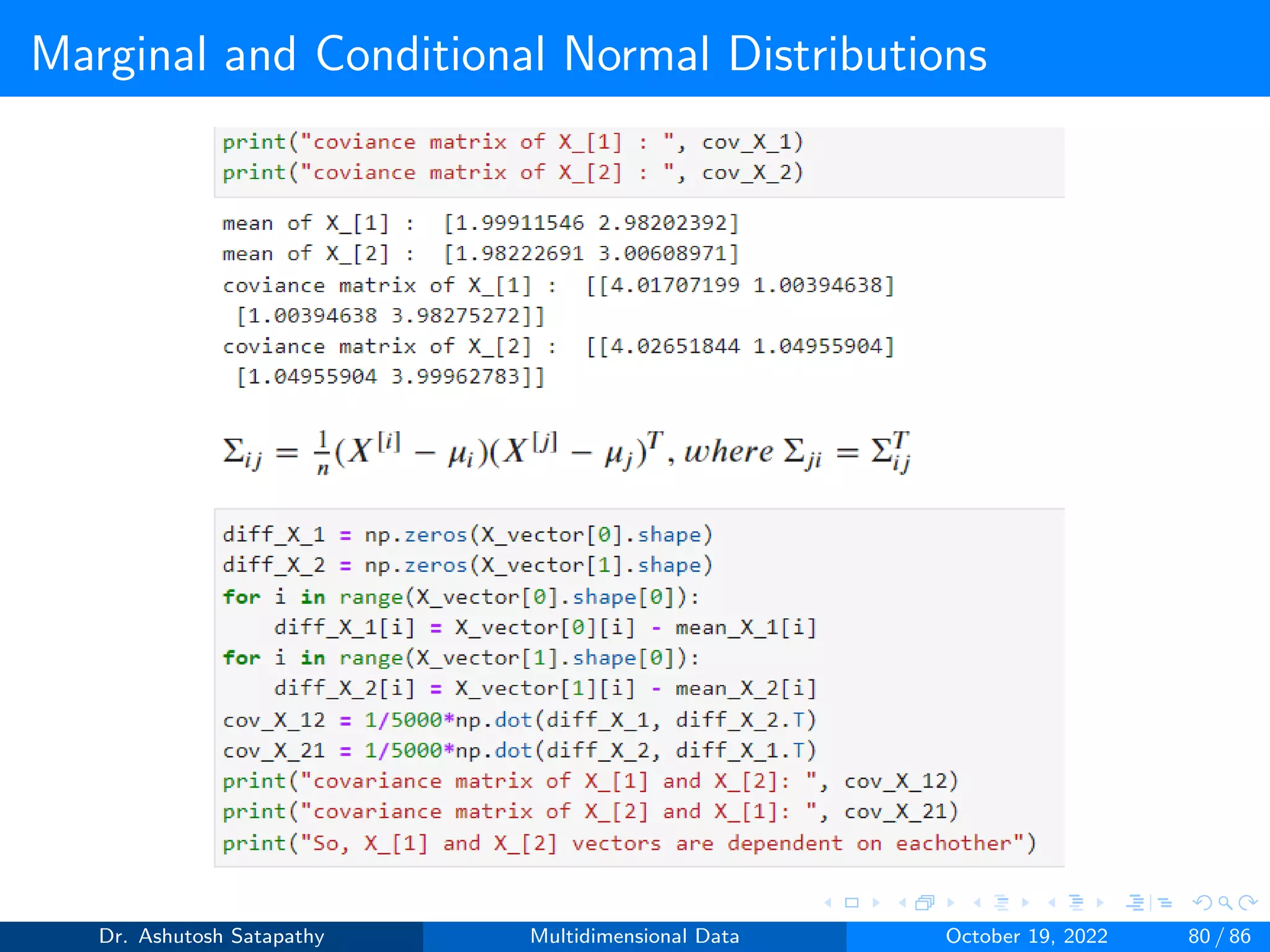
3 The (between) covariance matrix cov(X[1], X[2]) of X[1] and X[2]
is the d1xd2 submatrix Σ12 of.
Σ =
Σ1 Σ12
ΣT
12 Σ2
(25)
The marginal distributions of normal random vectors are normal with
means and covariance matrices of the original random vectors.
Dr. Ashutosh Satapathy Multidimensional Data October 19, 2022 72 / 86](https://image.slidesharecdn.com/multidimensionaldata-221019141857-58826018/75/Multidimensional-Data-72-2048.jpg)
![Marginal and Conditional Normal Distributions
Result 1.5
Assume that X[1], X[2] and X are given by Equation 24 for some d1, d2
d such that d1 + d2 = d. Assume also that X ∼ N(µ, Σ) and that Σ1
and Σ2 are invertible.
If X[1] and X[2] are independent. The covariance matrix Σ12 of
X[1] and X[2] satisfies
Σ12 = 0d1xd2 (26)
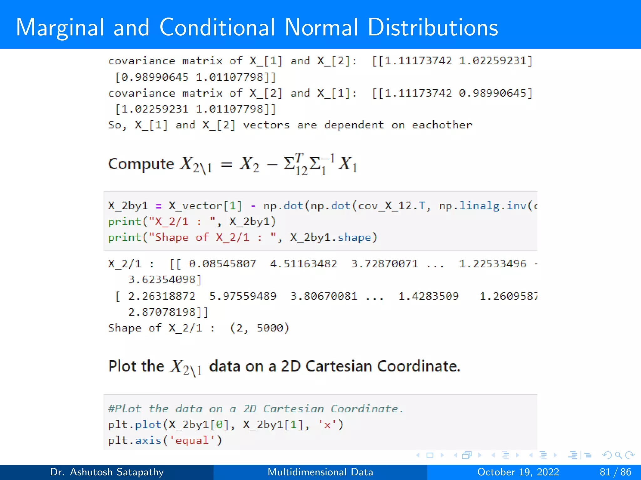
Assume that Σ12 ̸= 0d1×d2
. Put X21 = X2 -Σ12
TΣ1
-1X1. Then
X21 is a d2-dimensional random vector which is independent of X1
and X21 ∼N(µ21, Σ21) with
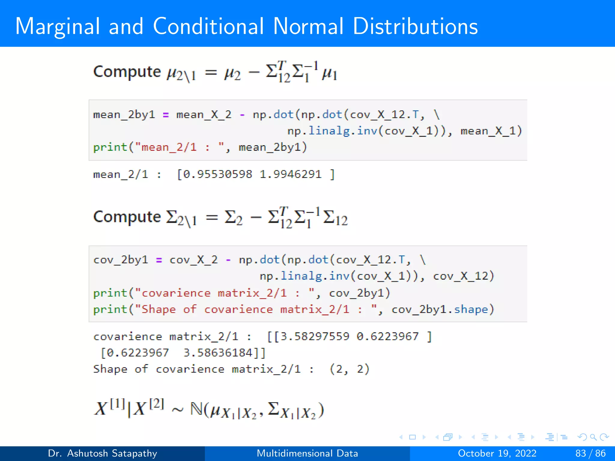
µ21 = µ2 − ΣT
12Σ−1
1 µ1 and Σ2/1 = Σ2 − ΣT
12Σ−1
1 Σ12 (27)
Dr. Ashutosh Satapathy Multidimensional Data October 19, 2022 73 / 86](https://image.slidesharecdn.com/multidimensionaldata-221019141857-58826018/75/Multidimensional-Data-73-2048.jpg)
![Marginal and Conditional Normal Distributions
Result 1.5 (Continue)
Let (X[1] | X[2]) be the conditional random vector X[1] given X[2].
Then (X[1] | X[2]) ∼ N(µX1 | X2
, ΣX1 | X2
)
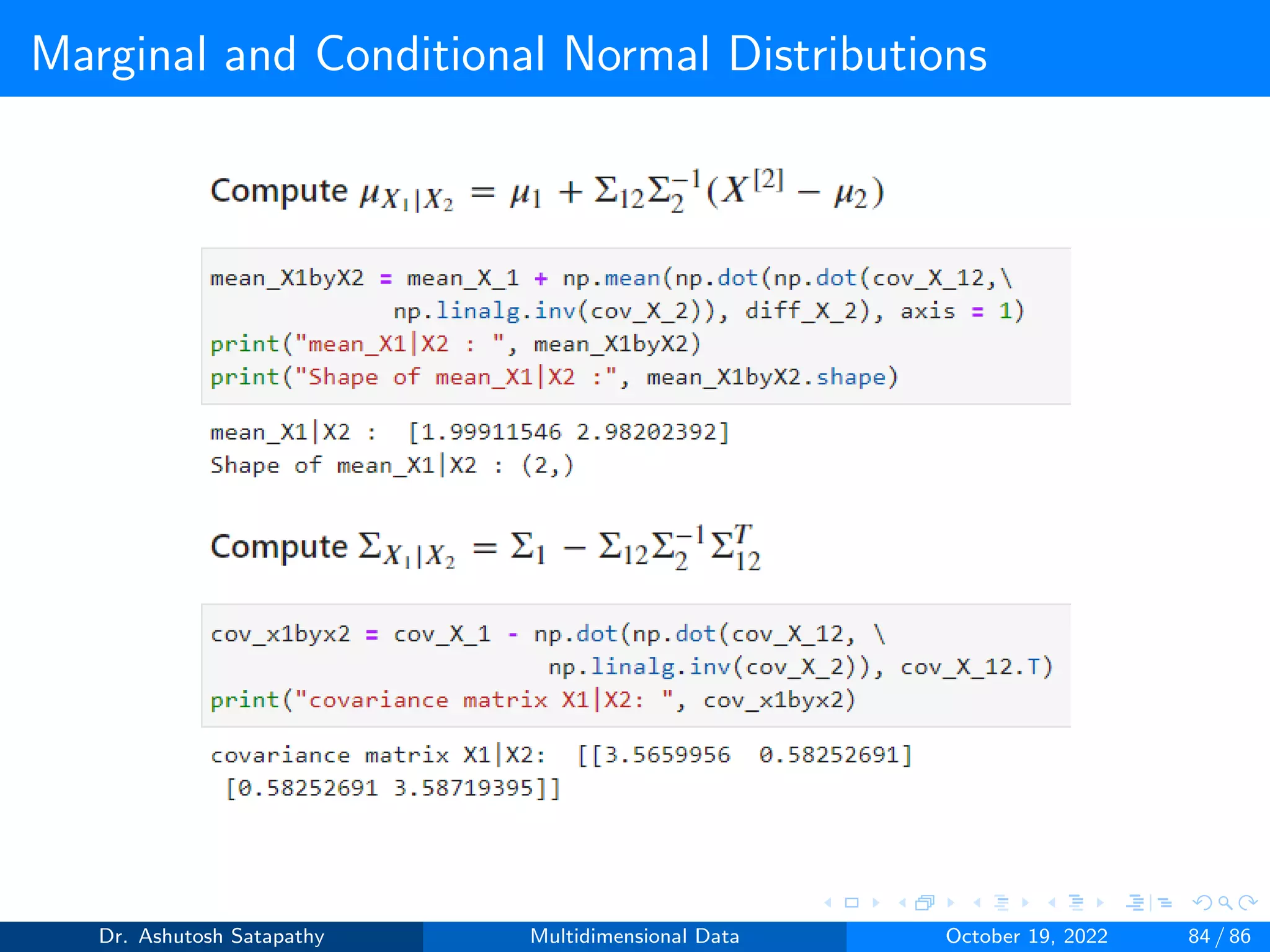
µX1|X2
= µ1 + Σ12Σ−1
2 (X[2]
− µ2) (28)
ΣX1|X2
= Σ1 − Σ12Σ−1
2 ΣT
12 (29)
The first property specifies independence always implies uncorrelated
-ness, and for the normal distribution, the converse holds too. The
second property shows how one can uncorrelate the vectors X[1] and
X[2]. The last property is about the adjustments that are needed when
the sub-vectors have a non-zero covariance matrix.
Dr. Ashutosh Satapathy Multidimensional Data October 19, 2022 74 / 86](https://image.slidesharecdn.com/multidimensionaldata-221019141857-58826018/75/Multidimensional-Data-74-2048.jpg)

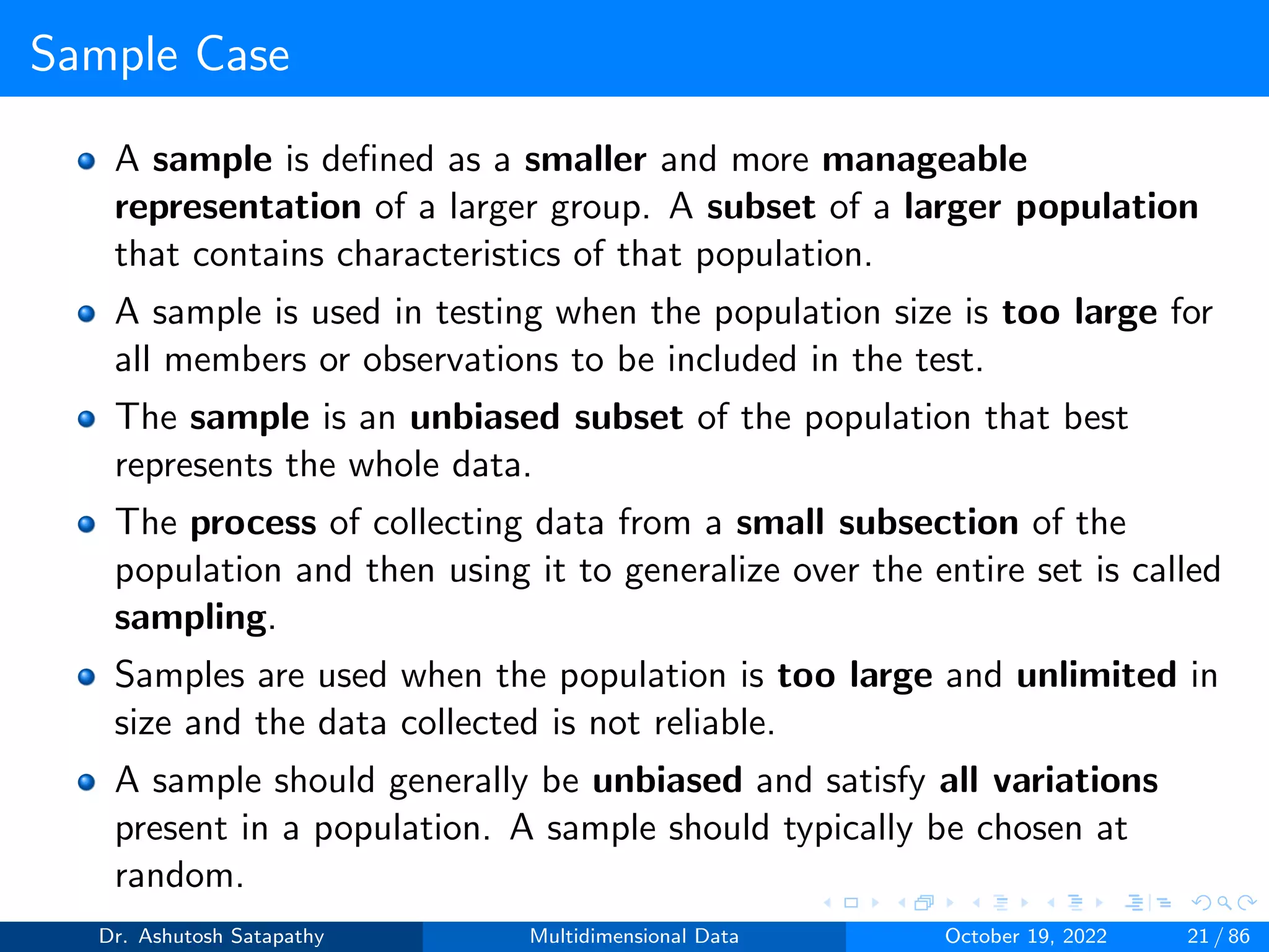
The document discusses multidimensional data analysis by Dr. Ashutosh Satapathy, covering key topics such as multivariate problems, visualization techniques, and the understanding of multivariate random vectors. It emphasizes the evolution of methods for analyzing high-dimensional data, highlighting the challenges posed by large dimensionality and low sample sizes. The document also explores various visualization tools, including three-dimensional scatter plots and parallel coordinate plots, to reveal data structures and relationships effectively.


![[DSC Europe 25] Aleksandra Dragicevic - AI-Boosted Research in Healthcare: Fr...](https://cdn.slidesharecdn.com/ss_thumbnails/iqwngszurf2r7pi1lnnj-4-aleksandra-dragicevic-ad-dsc-europe-conference-20-251208151905-37c3238a-thumbnail.jpg?width=640&height=640&fit=bounds)
![[DSC Europe 25] Jovan Bogicevic - Legacy to AI-Driven Defense: Transforming D...](https://cdn.slidesharecdn.com/ss_thumbnails/rsarluadt563hntyfc8q-3-251211083849-3e7bc4c0-thumbnail.jpg?width=640&height=640&fit=bounds)
![[DSC Europe 25] Dusan Nesic - Securing Tomorrow’s Infrastructure: Why Cyber-P...](https://cdn.slidesharecdn.com/ss_thumbnails/qikbszfftyowjm2q6duw-1-251211083848-8f2ead6b-thumbnail.jpg?width=640&height=640&fit=bounds)

![[DSC Europe 25] Ivan Peric - Intelligence Swarm Logic and Techno-Functional M...](https://cdn.slidesharecdn.com/ss_thumbnails/7my7c97fsduiccadgavw-2-251212103249-5a03f7c6-thumbnail.jpg?width=640&height=640&fit=bounds)

![[DSC Europe 25] Marija Vlajkovic & Andrea Radonjanin - Integration of AI tool...](https://cdn.slidesharecdn.com/ss_thumbnails/qf1jrglttoc3bm8s3aop-final-integration-of-ai-tools-251208151905-394f3a6a-thumbnail.jpg?width=640&height=640&fit=bounds)
![[DSC Europe 25] Bassam Maharmeh - Artificial Intelligence: Opportunities and ...](https://cdn.slidesharecdn.com/ss_thumbnails/thhfmr2fqpawzj7hsjpg-5-251211083048-2c23204f-thumbnail.jpg?width=640&height=640&fit=bounds)


![[DSC Europe 25] Sara Polak - The Archaeology of Innovation: AI as the Next Cr...](https://cdn.slidesharecdn.com/ss_thumbnails/7ecbscdnt8mlcuqbd2ln-2-sara-polak-ai-creative-industries-251208152533-aa1fcf54-thumbnail.jpg?width=640&height=640&fit=bounds)
![[DSC Europe 25] Branko Dzakula - From Defense to Attack: How AI Redefines Cyb...](https://cdn.slidesharecdn.com/ss_thumbnails/80bdzdxpr3ky2g0qvyk9-8-251211083048-ce5fc1ee-thumbnail.jpg?width=640&height=640&fit=bounds)
![[DSC Europe 25] Kaja Kandare - LLM as a judge.pptx](https://cdn.slidesharecdn.com/ss_thumbnails/arxyccaxsdsd1ba99wjw-7-251212104007-2b4e3f64-thumbnail.jpg?width=640&height=640&fit=bounds)
![[DSC Europe 25] Vladimir Jelic - The AI-Driven Security Shift From Reactive D...](https://cdn.slidesharecdn.com/ss_thumbnails/6g5gj25mtjwayniqem1t-6-251209104645-7a5a5fc6-thumbnail.jpg?width=640&height=640&fit=bounds)
![[DSC Europe 25] Dobrica Cosic - Savings by the Second: How Dynamic Pricing an...](https://cdn.slidesharecdn.com/ss_thumbnails/znp09f3smtqz3w2sq6wn-1-dobrica-cosic-savings-by-the-second-how-dynamic-pricing-and-smart-data-are-bu-251208151905-26e6f41e-thumbnail.jpg?width=640&height=640&fit=bounds)
![[DSC Europe 25] Sara Polak - The Ancient Operating System: What Archaeology T...](https://cdn.slidesharecdn.com/ss_thumbnails/3vch2p6tttdnwhsgazoz-3-sara-polak-smart-cities-251208152532-64404202-thumbnail.jpg?width=640&height=640&fit=bounds)
![[DSC Europe 25] Hans Kleinsman - The Compliance Gearbox: How Tax Tech Mediate...](https://cdn.slidesharecdn.com/ss_thumbnails/dxdytie1toel0hr90bjs-2-251212103250-174fdbe7-thumbnail.jpg?width=640&height=640&fit=bounds)