This document summarizes a presentation on using Python for scientific visualization. It discusses using libraries like Matplotlib, Mayavi, VTK, and custom frameworks for 2D and 3D plotting of scientific data. It provides examples of visualizing simulations in real-time, including particle simulations and the Mandelbrot set using just-in-time compilation with Numba for performance. The presentation also demonstrates interactive 3D visualization of MRI data and optimization techniques for Python like vectorization and GPU processing.

1. ScientificVisualization with GR
July 25, 2014 10:00 - 10:30
!
Berlin | EuroPython 2014 | Josef Heinen
MemberoftheHelmholtzAssociation

2. July 25, 2014 Josef Heinen, Forschungszentrum Jülich, Peter Grünberg Institute, Scientific IT Systems
Scientists need easy-to-use methods for:
✓ visualizing and analyzing two- and three-dimensional data sets, possibly with a
dynamic component
✓ creating publication-quality graphics and videos
✓ making glossy figures for high impact journals or press releases
2
Motivation

3. July 25, 2014 Josef Heinen, Forschungszentrum Jülich, Peter Grünberg Institute, Scientific IT Systems
✓ line / bar graphs, curve plots
✓ scatter plots
✓ contour plots
✓ vector / streamline plots
✓ surface plots, mesh rendering with iso-surface generation
✓ volume graphics
✓ molecule plots
3
Scientific plotting methods

4. July 25, 2014 Josef Heinen, Forschungszentrum Jülich, Peter Grünberg Institute, Scientific IT Systems
Matplotlib — de-facto standard (“workhorse”)
Mayavi2 (mlab) — powerful, but overhead fromVTK
VTK — versatile, but difficult to learn
Vispy, OpenGL — fast, but low(est)-level API
Qwt / QwtPlot3D — currently unmaintained
Scientific visualization solutions
4
qwt

5. July 25, 2014 Josef Heinen, Forschungszentrum Jülich, Peter Grünberg Institute, Scientific IT Systems
Problems so far
✓ separated 2D and (hardware accelerated) 3D world
✓ some graphics backends "only" produce pictures (figures)
➟ no presentation of continuous data streams
✓ bare minimum level of interoperability
➟ limited user interaction
✓ poor performance on large data sets
✓ APIs are partly device- and platform-dependent
5
… these problems are not specific to Python !

6. July 25, 2014 Josef Heinen, Forschungszentrum Jülich, Peter Grünberg Institute, Scientific IT Systems
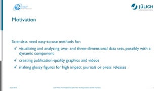
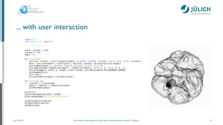
… so let’s get Python up and running
6
IPython + NumPy + SciPy + Bokeh + Numba + PyQt4 + Matplotlib
(* Anaconda (Accelerate) is a (commercial) Scientific Python distribution from Continuum Analytics
What else do we need?
% bash Anaconda-2.x.x-[Linux|MacOSX]-x86[_64].sh
% conda update conda
% conda update anaconda

7. July 25, 2014 Josef Heinen, Forschungszentrum Jülich, Peter Grünberg Institute, Scientific IT Systems
… achieve more Python performance
Numba: compiles annotated Python and NumPy code to LLVM (through
decorators)
✓ just-in-time compilation
✓ vectorization
✓ parallelization
NumbaPro: adds support for multicore and GPU architectures
7
(* Numba (Pro) is part of Anaconda (Accelerate), a (commercial) Python distribution from Continuum Analytics
performance

8. July 25, 2014 Josef Heinen, Forschungszentrum Jülich, Peter Grünberg Institute, Scientific IT Systems
… achieve more graphics performance and interop
GR framework: a universal framework for cross-platform visualization
✓ procedural graphics backend ➟ presentation of continuous data streams
✓ builtin device drivers ➟ coexistent 2D and 3D world
✓ interoperability with GUI toolkits ➟ good user interaction
8
% git clone https://github.com/jheinen/gr
% cd gr; make install
or
% pip install gr
or
% conda install -c https://conda.binstar.org/jheinen gr

9. July 25, 2014 Josef Heinen, Forschungszentrum Jülich, Peter Grünberg Institute, Scientific IT Systems
… so let’s complete our Scientific Python distribution
9
PyOpenGL + PyOpenCL + PyCUDA + PyGTK/wxWidgets
IPython + NumPy + SciPy + Bokeh + Numba + PyQt4 + GR framework
➟ more performance and interoperability

10. July 25, 2014 Josef Heinen, Forschungszentrum Jülich, Peter Grünberg Institute, Scientific IT Systems
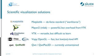
Presentation of continuous data streams in 2D ...
10
from numpy import sin, cos, sqrt, pi, array
import gr
!
def rk4(x, h, y, f):
k1 = h * f(x, y)
k2 = h * f(x + 0.5 * h, y + 0.5 * k1)
k3 = h * f(x + 0.5 * h, y + 0.5 * k2)
k4 = h * f(x + h, y + k3)
return x + h, y + (k1 + 2 * (k2 + k3) + k4) / 6.0
!
def damped_pendulum_deriv(t, state):
theta, omega = state
return array([omega, -gamma * omega - 9.81 / L * sin(theta)])
!
def pendulum(t, theta, omega)
gr.clearws()
... # draw pendulum (pivot point, rod, bob, ...)
gr.updatews()
!
theta = 70.0 # initial angle
gamma = 0.1 # damping coefficient
L = 1 # pendulum length
t = 0
dt = 0.04
state = array([theta * pi / 180, 0])
!
while t < 30:
t, state = rk4(t, dt, state, damped_pendulum_deriv)
theta, omega = state
pendulum(t, theta, omega)

11. July 25, 2014 Josef Heinen, Forschungszentrum Jülich, Peter Grünberg Institute, Scientific IT Systems
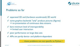
... with full 3D functionality
11
from numpy import sin, cos, array
import gr
import gr3
!
def rk4(x, h, y, f):
k1 = h * f(x, y)
k2 = h * f(x + 0.5 * h, y + 0.5 * k1)
k3 = h * f(x + 0.5 * h, y + 0.5 * k2)
k4 = h * f(x + h, y + k3)
return x + h, y + (k1 + 2 * (k2 + k3) + k4) / 6.0
!
def pendulum_derivs(t, state):
t1, w1, t2, w2 = state
a = (m1 + m2) * l1
b = m2 * l2 * cos(t1 - t2)
c = m2 * l1 * cos(t1 - t2)
d = m2 * l2
e = -m2 * l2 * w2**2 * sin(t1 - t2) - 9.81 * (m1 + m2) * sin(t1)
f = m2 * l1 * w1**2 * sin(t1 - t2) - m2 * 9.81 * sin(t2)
return array([w1, (e*d-b*f) / (a*d-c*b), w2, (a*f-c*e) / (a*d-c*b)])
!
def double_pendulum(theta, length, mass):
gr.clearws()
gr3.clear()
!
... # draw pivot point, rods, bobs (using 3D meshes)
!
gr3.drawimage(0, 1, 0, 1, 500, 500, gr3.GR3_Drawable.GR3_DRAWABLE_GKS)
gr.updatews()

12. July 25, 2014 Josef Heinen, Forschungszentrum Jülich, Peter Grünberg Institute, Scientific IT Systems
... in real-time
12
import wave, pyaudio
import numpy
import gr
!
SAMPLES=1024
FS=44100 # Sampling frequency
!
f = [FS/float(SAMPLES)*t for t in range(1, SAMPLES/2+1)]
!
wf = wave.open('Monty_Python.wav', 'rb')
pa = pyaudio.PyAudio()
stream = pa.open(format=pa.get_format_from_width(wf.getsampwidth()),
channels=wf.getnchannels(), rate=wf.getframerate(),
output=True)
!
...
!
data = wf.readframes(SAMPLES)
while data != '' and len(data) == SAMPLES * wf.getsampwidth():
stream.write(data)
amplitudes = numpy.fromstring(data, dtype=numpy.short)
power = abs(numpy.fft.fft(amplitudes / 65536.0))[:SAMPLES/2]
!
gr.clearws()
...
gr.polyline(SAMPLES/2, f, power)
gr.updatews()
data = wf.readframes(SAMPLES)

13. July 25, 2014 Josef Heinen, Forschungszentrum Jülich, Peter Grünberg Institute, Scientific IT Systems
... and in 3D
13
...
!
spectrum = np.zeros((256, 64), dtype=float)
t = -63
dt = float(SAMPLES) / FS
df = FS / float(SAMPLES) / 2 / 2
!
data = wf.readframes(SAMPLES)
while data != '' and len(data) == SAMPLES * wf.getsampwidth():
stream.write(data)
amplitudes = np.fromstring(data, dtype=np.short)
power = abs(np.fft.fft(amplitudes / 32768.0))[:SAMPLES/2]
!
gr.clearws()
spectrum[:, 63] = power[:256]
spectrum = np.roll(spectrum, 1)
gr.setcolormap(-113)
gr.setviewport(0.05, 0.95, 0.1, 1)
gr.setwindow(t * dt, (t + 63) * dt, 0, df)
gr.setscale(gr.OPTION_FLIP_X)
gr.setspace(0, 256, 30, 80)
gr3.surface((t + np.arange(64)) * dt, np.linspace(0, df, 256), spectrum, 4)
gr.setscale(0)
gr.axes3d(0.2, 0.2, 0, (t + 63) * dt, 0, 0, 5, 5, 0, -0.01)
gr.titles3d('t [s]', 'f [kHz]', '')
gr.updatews()
!
data = wf.readframes(SAMPLES)
t += 1

14. July 25, 2014 Josef Heinen, Forschungszentrum Jülich, Peter Grünberg Institute, Scientific IT Systems
... with user interaction
14
import gr3
from OpenGL.GLUT import *
# ... Read MRI data
width = height = 1000
isolevel = 100
angle = 0
!
def display():
vertices, normals = gr3.triangulate(data, (1.0/160, 1.0/160, 1.0/200), (-0.5, -0.5, -0.5), isolevel)
mesh = gr3.createmesh(len(vertices)*3, vertices, normals, np.ones(vertices.shape))
gr3.drawmesh(mesh, 1, (0,0,0), (0,0,1), (0,1,0), (1,1,1), (1,1,1))
gr3.cameralookat(-2*math.cos(angle), -2*math.sin(angle), -0.25, 0, 0, -0.25, 0, 0, -1)
gr3.drawimage(0, width, 0, height, width, height, gr3.GR3_Drawable.GR3_DRAWABLE_OPENGL)
glutSwapBuffers()
gr3.clear()
gr3.deletemesh(ctypes.c_int(mesh.value))
def motion(x, y):
isolevel = 256*y/height
angle = -math.pi + 2*math.pi*x/width
glutPostRedisplay()
glutInit()
glutInitWindowSize(width, height)
glutCreateWindow("Marching Cubes Demo")
!
glutDisplayFunc(display)
glutMotionFunc(motion)
glutMainLoop()

15. July 25, 2014 Josef Heinen, Forschungszentrum Jülich, Peter Grünberg Institute, Scientific IT Systems
Performance optimizations
✓ NumPy
module for handling multi-dimensional arrays (vector operations on ndarrays)
✓ Numba (Anaconda)
✓ just-in-time compilation driven by @autojit- or @jit-decorators (LLVM)
✓ vectorization of ndarray based functions (ufuncs) driven by @vectorize-decorators
✓ Numba Pro (Anaconda Accelerate)
✓ parallel loops and ufuncs
✓ execution of ufunfs on GPUs
✓ “Python” GPU kernels
✓ GPU optimized libraries (cuBLAS, cuFFT, cuRAND)
15
performance

16. July 25, 2014 Josef Heinen, Forschungszentrum Jülich, Peter Grünberg Institute, Scientific IT Systems
Particle simulation
16
import numpy as np
!
!
N = 300 # number of particles
M = 0.05 * np.ones(N) # masses
size = 0.04 # particle size
!
!
def step(dt, size, a):
a[0] += dt * a[1] # update positions
!
n = a.shape[1]
D = np.empty((n, n), dtype=np.float)
for i in range(n):
for j in range(n):
dx = a[0, i, 0] - a[0, j, 0]
dy = a[0, i, 1] - a[0, j, 1]
D[i, j] = np.sqrt(dx*dx + dy*dy)
!
... # find pairs of particles undergoing a collision
... # check for crossing boundary
return a
...
!
a[0, :] = -0.5 + np.random.random((N, 2)) # positions
a[1, :] = -0.5 + np.random.random((N, 2)) # velocities
a[0, :] *= (4 - 2*size)
dt = 1. / 30
!
while True:
a = step(dt, size, a)
....
!
from numba.decorators import autojit
!
!
!
!
!
@autojit
!
!
!
!
!
!
!
!
!
!
!
!
!
!
!
!
!
!
!
!
!
!
!

17. July 25, 2014 Josef Heinen, Forschungszentrum Jülich, Peter Grünberg Institute, Scientific IT Systems
Mandelbrot set
17
from numbapro import vectorize
import numpy as np
!
@vectorize(['uint8(uint32, f8, f8, f8, f8, uint32, uint32, uint32)'], target='gpu')
def mandel(tid, min_x, max_x, min_y, max_y, width, height, iters):
pixel_size_x = (max_x - min_x) / width
pixel_size_y = (max_y - min_y) / height
!
x = tid % width
y = tid / width
!
real = min_x + x * pixel_size_x
imag = min_y + y * pixel_size_y
!
c = complex(real, imag)
z = 0.0j
!
for i in range(iters):
z = z * z + c
if (z.real * z.real + z.imag * z.imag) >= 4:
return i
!
return 255
!
!
def create_fractal(min_x, max_x, min_y, max_y, width, height, iters):
tids = np.arange(width * height, dtype=np.uint32)
return mandel(tids, np.float64(min_x), np.float64(max_x), np.float64(min_y),
np.float64(max_y), np.uint32(height), np.uint32(width),
np.uint32(iters))

18. July 25, 2014 Josef Heinen, Forschungszentrum Jülich, Peter Grünberg Institute, Scientific IT Systems
Success stories (I)
18
Live Display for
KWS-2 small-angle neutron diffractometer
operated by JCNS at FRM II

19. July 25, 2014 Josef Heinen, Forschungszentrum Jülich, Peter Grünberg Institute, Scientific IT Systems
Success stories (II)
19
World’s most powerful laboratory small-
angle X-ray scattering facility at
Forschungszentrum Jülich
GR (embedded into Qt4)
as a replacement for a
proprietary solution

20. July 25, 2014 Josef Heinen, Forschungszentrum Jülich, Peter Grünberg Institute, Scientific IT Systems
Success stories (III)
20
NICOS
a network-based control system
written for neutron scattering
instruments at the FRM II
GR (qtgr) as a
replacement for
PyQwt

21. July 25, 2014 Josef Heinen, Forschungszentrum Jülich, Peter Grünberg Institute, Scientific IT Systems
Case study
21
BornAgain
A software to simulate and fit neutron and
x-ray scattering at grazing incidence
(GISANS and GISAXS), using distorted-
wave Born approximation (DWBA)
Nframes = 100
radius = 1
height = 4
distance = 5
!
def RunSimulation():
# defining materials
mAir = HomogeneousMaterial("Air", 0.0, 0.0)
mSubstrate = HomogeneousMaterial("Substrate", 6e-6, 2e-8)
mParticle = HomogeneousMaterial("Particle", 6e-4, 2e-8)
# collection of particles
cylinder_ff = FormFactorCylinder(radius, height)
cylinder = Particle(mParticle, cylinder_ff)
particle_layout = ParticleLayout()
particle_layout.addParticle(cylinder)
# interference function
interference = InterferenceFunction1DParaCrystal(distance, 3 * nanometer)
particle_layout.addInterferenceFunction(interference)
# air layer with particles and substrate form multi layer
air_layer = Layer(mAir)
air_layer.setLayout(particle_layout)
substrate_layer = Layer(mSubstrate)
multi_layer = MultiLayer()
multi_layer.addLayer(air_layer)
multi_layer.addLayer(substrate_layer)
# build and run experiment
simulation = Simulation()
simulation.setDetectorParameters(250, -4*degree, 4*degree, 250, 0*degree, 8*degree)
simulation.setBeamParameters(1.0 * angstrom, 0.2 * degree, 0.0 * degree)
simulation.setSample(multi_layer)
simulation.runSimulation()
return simulation.getIntensityData().getArray()
def SetParameters(i):
radius = (1. + (3.0/Nframes)*i) * nanometer
height = (1. + (4.0/Nframes)*i) * nanometer
distance = (10. - (1.0/Nframes)*i) * nanometer
!
for i in range(100):
SetParameters(i)
result = RunSimulation()
gr.pygr.imshow(numpy.log10(numpy.rot90(result, 1)), cmap=gr.COLORMAP_PILATUS)
GR (pygr) as a
replacement for
matplotlib

22. July 25, 2014 Josef Heinen, Forschungszentrum Jülich, Peter Grünberg Institute, Scientific IT Systems
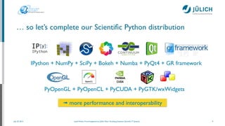
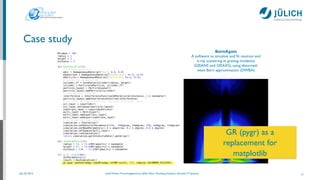
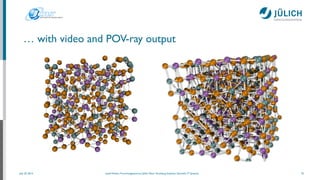
Comparison of the source code
if __name__ == '__main__':
files = []
fig = pylab.figure(figsize=(5,5))
ax = fig.add_subplot(111)
for i in range(Nframes):
SetParameters(i)
result = RunSimulation() + 1 # for log scale
ax.cla()
im = ax.imshow(numpy.rot90(result, 1), vmax=1e3,
norm=matplotlib.colors.LogNorm(),
extent=[-4.0, 4.0, 0, 8.0])
fname = '_tmp%03d.png'%i
fig.savefig(fname)
files.append(fname)
!
os.system("mencoder 'mf://_tmp*.png' -mf type=png:fps=10 -ovc lavc -lavcopts vcodec=wmv2 -oac copy -o animation.mpg")
os.system("rm _tmp*")
22
if __name__ == '__main__':
for i in range(Nframes):
SetParameters(i)
result = RunSimulation() + 1 # for log scale
gr.pygr.imshow(numpy.log10(numpy.rot90(result, 1)), cmap=gr.COLORMAP_PILATUS)
export GKS_WSTYPE=mov

23. July 25, 2014 Josef Heinen, Forschungszentrum Jülich, Peter Grünberg Institute, Scientific IT Systems
Conclusion
✓ The use of Python with the GR framework and Numba (Pro) extensions allows the realization
of high-performance visualization applications in scientific and technical environments
✓ The GR framework can seamlessly be integrated into any Python environment, e.g.Anaconda,
by using the ctypes mechanism
✓ Conda / Anaconda provide an easy to manage / ready-to-use Python distribution that can be
enhanced by the use of the GR framework with its functions for real-time or 3D visualization
applications
23
What’s next?

24. July 25, 2014 Josef Heinen, Forschungszentrum Jülich, Peter Grünberg Institute, Scientific IT Systems
Coming soon: Python moldyn package …
24

25. July 25, 2014 Josef Heinen, Forschungszentrum Jülich, Peter Grünberg Institute, Scientific IT Systems
… with video and POV-ray output
25

26. July 25, 2014 Josef Heinen, Forschungszentrum Jülich, Peter Grünberg Institute, Scientific IT Systems
… in highest resolution
26

27. July 25, 2014 Josef Heinen, Forschungszentrum Jülich, Peter Grünberg Institute, Scientific IT Systems
Future plans: combine the power of matplotlib and GR
matplotlib backend
Idea: use GR as a
matplotlib backend
➟ speed up matplotlib
… there are even
more challenges, e.g an
integration of bokeh

28. July 25, 2014 Josef Heinen, Forschungszentrum Jülich, Peter Grünberg Institute, Scientific IT Systems
Resources
✓ Website: http://gr-framework.org
✓ Git Repository: http://github.com/jheinen/gr
✓ PyPI: https://pypi.python.org/pypi/gr
✓ Binstar: https://binstar.org/jheinen/gr
✓ Talk: ScientificVisualization with GR
28

29. July 25, 2014 Josef Heinen, Forschungszentrum Jülich, Peter Grünberg Institute, Scientific IT Systems
Visualization software could be even better if …
✓ the prerequisites for an application would be described in terms of usability,
responsiveness and interoperability (instead of list of software dependencies)
✓ native APIs would be used instead of GUI toolkits
✓ release updates would not break version compatibility
29
Closing words

30. July 25, 2014 Josef Heinen, Forschungszentrum Jülich, Peter Grünberg Institute, Scientific IT Systems
Thank you for your attention
Contact:
j.heinen@fz-juelich.de
@josef_heinen!
!
Thanks to:
Florian Rhiem, Ingo Heimbach, Christian Felder, David Knodt, Jörg
Winkler, Fabian Beule, Marcel Dück, Marvin Goblet, et al.
30