DDU Workshop Day-2 presentation (1).pptx

Friday, October 11, 2024 1
National Workshop on Python Programming and
its Applications
(September 18-20, 2024)
Dr. Nilam
Department of Applied Mathematics,
Delhi Technological University
Bawana Road, Delhi
Email: drnilam@dtu.ac.in

Drawing diverse shapes using code and Turtle
“Turtle” is a Python feature like a drawing board, which lets us command a turtle to
draw all over it! We can use functions like turtle.forward(…) and turtle.right(…) which
can move the turtle around. Commonly used turtle methods are :
Method Parameter Description
Turtle() None Creates and returns a new turtle object
forward() amount Moves the turtle forward by the specified amount
backward() amount Moves the turtle backward by the specified amount
right() angle Turns the turtle clockwise
left() angle Turns the turtle counterclockwise
penup() None Picks up the turtle’s Pen
goto() x, y Move the turtle to position x,y
begin_fill() None Remember the starting point for a filled polygon
end_fill() None Close the polygon and fill with the current fill color
color() Color name Changes the color of the turtle’s pen
fillcolor() Color name Changes the color of the turtle will use to fill a polygon
shape() shapename Should be ‘arrow’, ‘classic’, ‘turtle’ or ‘circle’

Plotting using Turtle
The roadmap for executing a turtle program follows 4 steps:
1. Import the turtle module
2. Create a turtle to control.
3. Draw around using the turtle methods.
4. Run turtle.done().
• So as stated above, before we can use turtle, we need to import it. We import it as
import turtle
• Now we need to create a new drawing board(window) and a turtle. Let’s call the
window as wn and the turtle as skk. So we code as:
wn = turtle.Screen()
wn.bgcolor("light green")
wn.title("Turtle")
skk = turtle.Turtle()
• we need to move the turtle. To move forward 100 pixels in the direction skk is facing
skk.forward(100)
• Now we complete the program with the done() function and We’re done!
turtle.done()

Shape 1: Square
import turtle
skk = turtle.Turtle() output:
for i in range(4):
skk.forward(50)
skk.right(90)
turtle.done()
Shape 2: Star
import turtle
star = turtle.Turtle()
star.right(75)
star.backward(100)
for i in range(4):
star.forward(100) output:
star.right(144) # This is to make the star shape
turtle.done()

5
Shape 3: Hexagon
import turtle
polygon = turtle.Turtle()
num_sides = 6 output:
side_length = 70
angle = 360.0 / num_sides
for i in range(num_sides):
polygon.forward(side_length)
polygon.right(angle)
turtle.done()
Shape 4: Filled color circle
import turtle
# Set up the turtle screen and set the background color to white
screen = turtle.Screen()
screen.bgcolor("white")
# Create a new turtle and set its speed to the fastest possible
pen = turtle.Turtle()
pen.speed(0) output:
# Set the fill color to red
pen.fillcolor("red")
pen.begin_fill()
# Draw the circle with a radius of 100 pixels
pen.circle(100)
# End the fill and stop drawing
pen.end_fill()
pen.hideturtle()
# Keep the turtle window open until it is manually closed
turtle.done()
Friday, October 11, 2024

Matplotlib:
• Matplotlib is a comprehensive library for creating
static, animated and interactive visualizations in
Python.
• Usage: Matplotlib /Pandas is mostly used for quick plotting of
Pandas Data Frames and time series analysis.
Pros and Cons of Matplotlib:
• Pro: Easy to setup and use.
• Pro: Very customizable.
• Con: Visual presentation tends to be simple
compared to other tools.

Installing Matplotlib should be straightforward.
Sample code for installing packages:
1. Functional/MATLAB Approach (Non-Pythonic)
● Most common way of Matplotlib.
● Pro: Easy approach for interactive use.
● Con- Not pythonic: Relies on global functions (where variables are declared outside of functions) and displays
global figures.
2. Object-Oriented Approach (Pythonic)
● Recommended way to use Matplotlib.
● Pro: Pythonic is object-oriented (you can build plots explicitly using methods of the figure and the
classes it contains.
Matplotlib - 2 Approaches to Plotting

Matplotlib-Non-Pythonic:
•Example: Combining Line & Scatter Plots From Categorical Variables
import matplotlib.pyplot as plt output:
names = ['grade_a', 'grade_b', 'grade_c', 'grade_d', 'grade_f']
values = [10, 30, 20, 8, 3]
plt.plot(names, values, 'm-') # 'm-' specifies a magenta line
plt.scatter(names, values) # Scatter plot overlay
plt.xlabel('Grades')
plt.ylabel('Values')
plt.title('Grades vs Values')
plt.show()

Matplotlib-Non-Pythonic:
Example: Simple Line Plot & Bar Plot
import matplotlib.pyplot as plt
import numpy as np output:
# f is the canvas object, can contain several plots
# i.e. axes objects (ax)
f, ax = plt.subplots() # returns tuple: (figure, axes)
values = [10, 30, 20, 8, 3]
group_mean = np.mean(values) / 4
# Add a horizontal line denoting average
ax.axhline(group_mean, linestyle='--', color='r')
# Plot data as parameters
ax.plot([1, 2, 3, 4], [5, 2, 8, 7])
ax.hist(np.random.randint(1, 4, 10))
plt.show()

Pyplot:
• Pyplot is a state-based interface to a Matplotlib module which provides a MATLAB-
like interface. subplots() function in Python simplifies the creation of multiple
subplots Matplotlib within a single figure, allowing for organized and simultaneous
visualization of various datasets or plots.
• Here is an example of a simple Python code to plot a graph using the Matplotlib
library.
plt.plot([1, 2, 3, 4], [16, 4, 1, 8]) output:
plt.show()

11
Subplots:
• Syntax: matplotlib.pyplot.subplots(nrows=1, ncols=1, sharex=False, sharey=False,
squeeze=True, subplot_kw=None, gridspec_kw=None, **fig_kw)
• Parameters: This method accept the following parameters that are described below:
• nrows, ncols : These parameter are the number of rows/columns of the subplot grid.
• sharex, sharey : These parameter controls sharing of properties among x (sharex) or y (sharey)
axes.
• squeeze : This parameter is an optional parameter and it contains boolean value with default
as True.
• num: This parameter is the pyplot.figure keyword that sets the figure number or label.
• subplot_kwd: This parameter is the dict with keywords passed to the add_subplot call used to
create each subplot.
• gridspec_kw: This parameter is the dict with keywords passed to the GridSpec constructor
used to create the grid the subplots are placed on.
• Returns: This method return the following values.
• fig : This method return the figure layout.
• ax : This method return the axes.Axes object or array of Axes objects.

Stacking Subplots in Two Directions
# Implementation of matplotlib function
import numpy as np
# First create some toy data:
x = np.linspace(0, 2 * np.pi, 400)
y1 = np.sin(x)
y2 = np.sin(x**2)
y3 = y1**2
y4 = y2**2 output:
fig, ax = plt.subplots(nrows=2, ncols=2)
ax[0, 0].plot(x, y1, c='red')
ax[0, 1].plot(x, y2, c='red')
ax[1, 0].plot(x, y3, c='blue')
ax[1, 1].plot(x, y3, c='blue')
ax[0, 0].set_title('Simple plot with sin(x)')
ax[0, 1].set_title('Simple plot with sin(x**2)')
ax[1, 0].set_title('Simple plot with sin(x)**2')
ax[1, 1].set_title('Simple plot with sin(x**2)**2')
fig.suptitle('Stacked subplots in two direction')
plt.show()
Stacking subplots in two directions

Eigenvalues and Eigenvectors in Python:
• The main built-in function in Python to solve the eigenvalue/eigenvector problem
for a square array is the eig function in numpy.linalg.
• Let’s see how we can use it.
Example- Compute the eigenvalues and eigenvectors for matrix .
import numpy as np
from numpy.linalg import eig
a = np.array([[2, 2, 4], [1, 3, 5], [2, 3, 4]])
w,v=eig(a)
print('E-value:', w)
print('E-vector', v)
Output:
E-value: [ 8.80916362 0.92620912 -0.73537273]
E-vector [[-0.52799324 -0.77557092 -0.36272811]
[-0.604391 0.62277013 -0.7103262 ]
[-0.59660259 -0.10318482 0.60321224]]

14
Solving a System of Coupled Differential Equations:
• Since we have all the theoretical knowledge and understood all the important concepts that we required
before beginning to solve an equation. We are now ready to get hands-on experience by implementing a
simple example to solve a coupled differential equation using NumPy.
import numpy as np
from scipy.integrate import odeint
def coupled_differential_equations(y, t, k, b):
x, v = y
dxdt = v
dvdt = -k * x - b * v
return [dxdt, dvdt]
y0 = [1.0, 0.0]
k = 1.0
b = 0.2
t = np.linspace(0, 10, 1000)
solutions = odeint(coupled_differential_equations, y0, t, args=(k, b))
x_values = solutions[:, 0]
v_values = solutions[:, 1]
plt.plot(t, x_values, label='Position x')
plt.plot(t, v_values, label='Velocity v')
plt.xlabel('Time')
plt.ylabel('Position / Velocity')
plt.legend()
plt.title('Coupled Differential Equations: Simple Harmonic Oscillator with Damping')
plt.show()

•The system of coupled differential equations for the straightforward harmonic
oscillator with damping is represented by the function coupled differential
equations, which we first defined in line 4. The four arguments the function needs
are y, t, k, and b. y is a list that contains the oscillator’s position and velocity at the
moment. The time is shown by the symbol t.
•The spring constant is k, while the damping factor is b.
•The coupled differential equations function accepts the args=(k, b) parameter,
which contains the values of k and b.

Define and call functions in Python:
• In Python, functions are defined using def statements, with parameters enclosed in
parentheses (), and return values are indicated by the return statement.
def function_name(parameter1, parameter2...):
do_something
return return_value
• To call a defined function, use the following syntax
function_name(argument1, argument2...)
Example:
def add(a, b):
x = a + b
return x
x = add(3, 4)
print(x)

Sympy : Symbolic Mathematics in Python:
• SymPy is a Python library for symbolic mathematics.
• Using SymPy as a calculator
SymPy defines three numerical types: Real, Rational and Integer.
import sympy as sym
>>> a = sym.Rational(1, 2)
>>> a
1/2
>>> a*2
1
• Symbols
In contrast to other Computer Algebra Systems, in SymPy we have to declare symbolic
variables explicitly:
x = sym.Symbol('x')
>>> y = sym.Symbol('y')
x + y + x - y
2*x
>>> (x + y) ** 2
(x + y)**2

• Expand:
Use this to expand an algebraic expression. It will try to denest powers and multiplications:
x = sym.Symbol('x')
y = sym.Symbol(‘y')
sym.expand((x + y) ** 3)
3 2 2 3
x + 3*x *y + 3*x*y + y
>>> 3 * x * y ** 2 + 3 * y * x ** 2 + x ** 3 + y ** 3
3 2 2 3
x + 3*x *y + 3*x*y + y
• Limits:
Limits are easy to use in SymPy, they follow the syntax limit(function, variable, point), so to compute the limit
of as , you would issue limit(f, x, 0):
x = sym.Symbol('x')
sym.limit(sym.sin(x) / x, x, 0)
1
we can also calculate the limit at infinity:
sym.limit(x, x, sym.oo)
oo

• Differentiation:
You can differentiate any SymPy expression using diff(func, var).
Examples:
x = sym.Symbol('x')
sym.diff(sym.sin(2 * x), x)
2*cos(2*x)
Higher derivatives can be calculated using the diff(func, var, n) method:
sym.diff(sym.sin(2 * x), x, 3)
-8*cos(2*x)
• Integration:
SymPy has support for indefinite and definite integration of transcendental elementary and special functions
via integrate() facility.
sym.integrate(sym.log(x), x)
x*log(x) – x
It is possible to compute definite integral
sym.integrate(sym.cos(x), (x, -sym.pi / 2, sym.pi / 2))
2
Also improper integrals are supported as well:
sym.integrate(sym.exp(-x), (x, 0, sym.oo))
1

Solution of ordinary differential equations:
• To numerically solve a system of ODEs, use a SciPy ODE solver such as solve_ivp. we
can also use SymPy to create and then lambdify() an ODE to be solved numerically
using SciPy’s as solve_ivp as described below in Numerically Solve an ODE in SciPy.
• Here is an example of solving the ordinary differential equation algebraically using
dsolve(). we can then use checkodesol() to verify that the solution is correct.
• Use SymPy to solve an ordinary differential equation (ODE) algebraically. For
example, solving y″(x)+9y(x)=0 yields y(x)=C1sin⁡
(3x)+C2cos⁡
(3x).
from sympy import Function, dsolve, Derivative, checkodesol
from sympy.abc import x
y = Function('y')
# Solve the ODE
result = dsolve(Derivative(y(x), x, x) + 9*y(x), y(x))
print(result) # Eq(y(x), C1*sin(3*x) + C2*cos(3*x))
# Check that the solution is correct
check = checkodesol(Derivative(y(x), x, x) + 9*y(x), result)
print(check) # (True, 0)

Computation of eigenvalues:
• To find the eigenvalues of a matrix, use eigenvals. eigenvals returns a dictionary
of eigenvalue: algebraic_multiplicity pairs (similar to the output of roots).
• M = Matrix([[3, -2, 4, -2], [5, 3, -3, -2], [5, -2, 2, -2], [5, -2, -3, 3]])
>>> M.eigenvals()
{-2: 1, 3: 1, 5: 2}
This means that M has eigenvalues -2, 3, and 5, and that the eigenvalues -2 and 3
have algebraic multiplicity 1 and that the eigenvalue 5 has algebraic multiplicity 2.
• To find the eigenvectors of a matrix, use eigenvects. eigenvects returns a list of
tuples of the form (eigenvalue, algebraic_multiplicity, [eigenvectors])

Simplification of expressions
• When we do not know anything about the structure of the expression, simplify() tries to apply
intelligent heuristics to make the input expression “simpler”.
• For example:
from sympy import simplify, cos, sin
>>> from sympy.abc import x, y
>>> a = (x + x**2)/(x*sin(y)**2 + x*cos(y)**2)
>>> a
(x**2 + x)/(x*sin(y)**2 + x*cos(y)**2)
>>> simplify(a)
x + 1
Factor
• This function collects additive terms of an expression with respect to a list of expression up to
powers with rational exponents
from sympy import symbols, factor
x, y = symbols('x y')
equation = x**2 - y**2
# Factorize the equation
factored_equation = factor(equation)
print(factored_equation)
output: (x-y)*(x+y)

23
Collecting
• factor() takes a polynomial and factors it into irreducible factors over the rational numbers. For
example
from sympy import collect, symbols
x = symbols('x')
expr = x**2 + 2*x + x**2
collected_expr = collect(expr, x)
print(collected_expr)
Output 2*x**2+ 2*x
Partial fraction decomposition
from sympy import symbols, apart
# Define the variable and the rational function
x = symbols('x')
rational_function = (3*x**2 + 5*x + 2) / (x**3 - x)
# Perform partial fraction decomposition
decomposed = apart(rational_function)
print(decomposed)
Output: 5*x/(x-1) – 2/x

Trigonometric simplification
• To simplify trigonometric expressions in Python, we can use the sympy library,
which provides a function called trigsimp(). This function simplifies trigonometric
expressions using various identities.
• Example:
from sympy import symbols, sin, cos, trigsimp
# Define the variable
x = symbols('x')
# Define the trigonometric expression
expr = sin(x)**2 + cos(x)**2
# Simplify the expression
simplified_expr = trigsimp(expr)
print(simplified_expr)
output: 1

Exponential and logarithms
• In Python, you can work with exponential and logarithmic functions using
the math and numpy libraries. Here are some basic examples:
• Using the math Module
The math module provides functions for both exponential and logarithmic calculations:
import math
# Exponential functions
exp_value = math.exp(2) # e^2
print(f"e^2 = {exp_value}")
# Logarithmic functions
log_value = math.log(10) # Natural log (base e)
print(f"ln(10) = {log_value}")
log10_value = math.log10(100) # Log base 10
print(f"log10(100) = {log10_value}")
Output: e^2 = 7.3890560989
ln(10) = 2.3025850929
log10(100) = 2.0

Using the numpy Library
• The numpy library offers more advanced functions, especially useful for array
operations:
import numpy as np
# Exponential functions
exp_array = np.exp([1, 2, 3]) # e^1, e^2, e^3
print(f"Exponential array: {exp_array}")
# Logarithmic functions
log_array = np.log([1, np.e, np.e**2]) # Natural log
print(f"Natural log array: {log_array}")
log10_array = np.log10([1, 10, 100]) # Log base 10
print(f"Log base 10 array: {log10_array}")
Output: Exponential array: [2.71828183 7.3890561 20.08553692]
Natural log array: [0. 1. 2.]
Log base 10 array: [0. 1. 2.]

Series expansion
• Series expansion, such as Taylor series, can be used to approximate functions. We
are using the sympy library:
• Example
import sympy as sp
# Define the variable and function
x = sp.symbols('x')
f = sp.sin(x)
### Compute the Taylor series expansion of f around x=0 up to the 5th
order###
taylor_series = sp.series(f, x, 0, 5)
print(taylor_series)
Output: x - x**3/6 + O(x**5)

Finite Differences in Python:
• Finite differences are used to approximate derivatives. Here
are some common methods using NumPy:
• Forward Difference
import numpy as np
def forward_difference(f, x, h):
return (f(x + h) - f(x)) / h
# Example usage
f = np.sin
x = np.pi / 4
h = 1e-5
print(forward_difference(f, x, h))
Output: 0.70710324456451

Central Difference:
import numpy as np
def central_difference(f, x, h):
return (f(x + h) - f(x - h)) / (2 * h)
# Define a sample function
def f(x):
return x**2
# Example usage
x = 2
h = 0.01
print(central_difference(f, x, h))
Output: 3.99999999997

Recursion in Python:
• The term Recursion can be defined as the process of defining something in terms of itself. In
simple words, it is a process in which a function calls itself directly or indirectly.
Syntax:
def func(): <--
|
| (recursive call)
|
func() ----
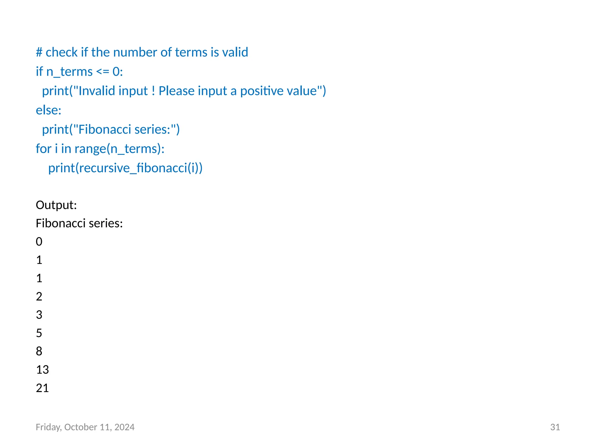
Example 1: A Fibonacci sequence is the integer sequence of 0, 1, 1, 2, 3, 5, 8….
# Program to print the fibonacci series upto n_terms
# Recursive function
def recursive_fibonacci(n):
if n <= 1:
return n
else:
return(recursive_fibonacci(n-1) + recursive_fibonacci(n-2))
n_terms = 10

# check if the number of terms is valid
if n_terms <= 0:
print("Invalid input ! Please input a positive value")
else:
print("Fibonacci series:")
for i in range(n_terms):
print(recursive_fibonacci(i))
Output:
Fibonacci series:
0
1
1
2
3
5
8
13
21

Printing:
• As we have already seen, SymPy can pretty print its output using Unicode
characters. This is a short introduction to the most common printing options
available in SymPy.
Printers:
• There are several printers available in SymPy. The most common ones are
• str
• srepr
• ASCII pretty printer
• Unicode pretty printer
• LaTeX
• MathML
• Dot
Setting up Pretty Printing
• If all you want is the best pretty printing, use the init_printing() function. This will
automatically enable the best printer available in your environment.
from sympy import init_printing
>>> init_printing()

• If we plan to work in an interactive calculator-type session,
the init_session() function will automatically import everything in SymPy, create
some common Symbols, setup plotting, and run init_printing().
from sympy import init_session
>>> init_session()
Example-

Pandas API for IO tools:
• The pandas I/O API is a set of top level reader functions accessed like
pandas.read_csv() that generally return a pandas object.
text files:
• The workhorse function for reading text files (a.k.a. flat files) is read_csv().
import pandas as pd
# Load the text file
df = pd.read_csv('/sample-1.txt', delimiter='t')
# Use 't' for tab-separated files, or ',' for CSV files
print(df.head()) # Display the first few rows
Output: Sample Document
0 Fusce convallis metus id felis luctus adipisci...
1 Nulla facilisi. Phasellus accumsan cursus veli...
2 Praesent ac massa at ligula laoreet iaculis. P...
3 Pellentesque egestas, neque sit amet convallis...
4 In enim justo, rhoncus ut, imperdiet a, venena...

csv files:
• The workhorse function for reading csv files (a.k.a. flat files) is read_csv().
import pandas as pd
# Load the text file
df = pd.read_csv('/industry.csv', delimiter='t')
# Use 't' for tab-separated files, or ',' for CSV files
print(df.head()) # Display the first few rows
Output: Industry
0 Accounting/Finance
1 Advertising/Public Relations
2 Aerospace/Aviation
3 Arts/Entertainment/Publishing
4 Automotive

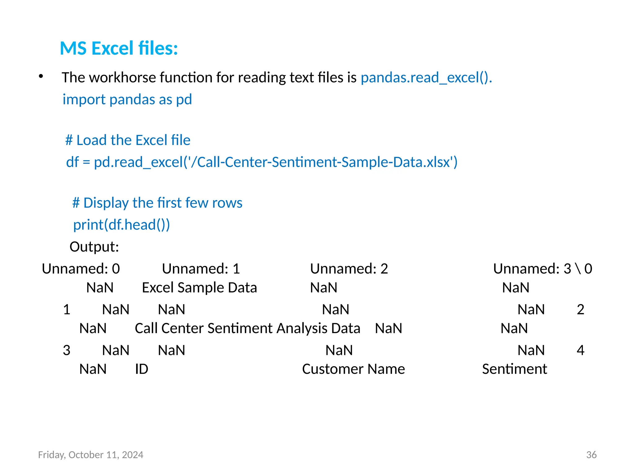
MS Excel files:
• The workhorse function for reading text files is pandas.read_excel().
import pandas as pd
# Load the Excel file
df = pd.read_excel('/Call-Center-Sentiment-Sample-Data.xlsx')
# Display the first few rows
print(df.head())
Output:
Unnamed: 0 Unnamed: 1 Unnamed: 2 Unnamed: 3 0
NaN Excel Sample Data NaN NaN
1 NaN NaN NaN NaN 2
NaN Call Center Sentiment Analysis Data NaN NaN
3 NaN NaN NaN NaN 4
NaN ID Customer Name Sentiment

Slides prepared by Mr. Sunil Kumar
Meena, Ph.D. Scholar, Department of
Applied Mathematics, DTU
THANK YOU

DDU Workshop Day-2 presentation (1).pptx

More Related Content

Similar to DDU Workshop Day-2 presentation (1).pptx

Recently uploaded

DDU Workshop Day-2 presentation (1).pptx