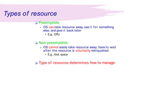
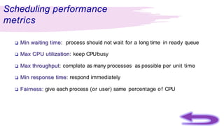
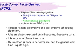
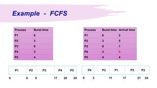
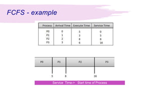
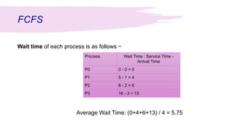
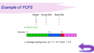
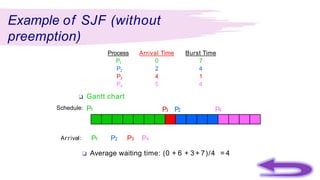
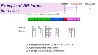
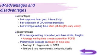
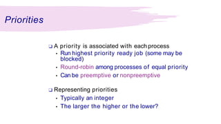
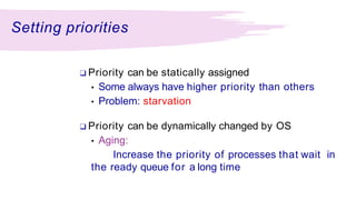
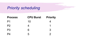
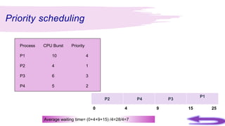
The document discusses various CPU scheduling algorithms including First-Come, First-Served (FCFS), Shortest Job First (SJF), Shortest Remaining Time First (SRTF), Round Robin (RR), and Priority Scheduling. It presents their characteristics, advantages, and disadvantages, along with examples illustrating their performance metrics such as average wait time, response time, and context switches. Additionally, it covers concepts like preemptible and non-preemptible resources, fairness, and the impact of time slices on scheduling efficiency.

1. Scheduling Algorithms
- INTRODUCTIO
N
- FCFS
- SJF
- SRTF
- RR
- PRIORITY
Dr.T.Revathi, PSGCAS
Scheduling Algorithms

2. Types of resource
❑ Preemptible
• OS can take resource away, use it for something
else, and give it back later
• E.g., CPU
❑ Non-preemptible
• OS cannot easily take resource away; have to wait
after the resource is voluntarily relinquished
• E.g., disk space
❑ Type of resource determines how to manage

3. Scheduling performance
metrics
❑ Min waiting time: process should not wait for a long time in ready queue
❑ Max CPU utilization: keep CPUbusy
❑ Max throughput: complete as many processes as possible per unit time
❑ Min response time: respond immediately
❑ Fairness: give each process (or user) same percentage of CPU

4. First-Come, First-Served
(FCFS)
❑ Simplest CPUscheduling algorithm
• First job that requests the CPUgets the
CPU
• Non preemptive /preemptive
❑ Implementation: FIFO queue
• It supports non-preemptive and pre-emptive scheduling
algorithm.
• Jobs are always executed on a first-come, first-serve basis.
• It is easy to implement and use.
• This method is poor in performance, and the general wait
time is quite high.

5. Example - FCFS
Process Burst time
P1 6
P2 3
P3 8
P4 3
P5 4
Process Burst time Arrival time
P1 6 2
P2 3 5
P3 8 1
P4 3 0
P5 4 4
P1 P2 P3 P4 P5
0 6 9 17 20 24
P4 P3 P1 P5 P2
0 3 11 17 21 24

6. FCFS - example
Service Time-> Start time of Process

7. FCFS
Process Wait Time : Service Time -
Arrival Time
P0 0 - 0 = 0
P1 5 - 1 = 4
P2 8 - 2 = 6
P3 16 - 3 = 13
Wait time of each process is as follows −
Average Wait Time: (0+4+6+13) / 4 = 5.75

8. Process Arrival Time Burst Time
P1 0 7
P2 0 4
P3 0 1
P4 0 4
Gantt chart
P1 P2 P3
P4
❑
Schedule:
❑ Average waiting time: (0 + 7 + 11+ 12)/4 = 7.5
Example of FCFS

9. SJF
• This is also known as shortest job first, or SJF
• This is a non-preemptive, pre-emptive scheduling
algorithm.
• Best approach to minimize waiting time.
• Easy to implement in Batch systems where required CPU
time is known in advance.
• Impossible to implement in interactive systems where
required CPU time is not known.
• The processer should know in advance how much time
process will take.

10. Shortest Job First
(SJF)
❑ Schedule the process with the shortest time
• FCFS if same time
❑ Advantages
• Minimizes average wait time. Provably optimal
❑ Disadvantages
• Not practical: difficult to predict burst time
• Possible: past predicts future
• May starve long jobs

11. Process Arrival Time Burst Time
P1 0 7
P2 2 4
P3 4 1
P4 5 4
❑ Gantt chart
Schedule: P1
❑ Average waiting time: (0 + 6 + 3 + 7)/4 = 4
Example of SJF (without
preemption)
P1 P2 P3 P4
P3 P2 P4
Arrival:

12. Shortest Remaining Time First (SRTF)
❑ I f new process arrives with shorter CPU
burst than the remaining for current
process, schedule new process
• SJF with preemption
❑ Advantage: reduces average waiting time

13. ❑ Gantt chart
❑ Average waiting time: (9 + 1 + 0 + 2)/4 = 3
Example of SRTF
P3 P2
Schedule: P1 P2 P4 P1
P1 P2
Arrival: P3 P4

14. Round-Robin
(RR)
❑ Practical approach to support time-sharing
❑ Run process for a time slice, then move to
back of FIFO queue
❑ Preempted if still running at end of time-slice
❑ How to determine time slice?

15. ❑ Gantt chart with time slice =3
❑ Average waiting time: (8 + 8 + 5 + 7)/4 = 7
❑ Average response time: (0 +1+5 +5)/4 =2.75
❑ # of context switches: 7
Example of RR: time
slice = 3
P1 P2 P3 P4
Arrival:
Queue:
P1 P1 P2 P2 P2 P1
P2 P1 P1 P1 P3
P3 P3 P4
P4 P2
P3 P4
P4 P2
P2 P1
P1
P2 P1 P4
P1 P4
P4

16. ❑ Gantt chart with time slice =1
❑ Average response time: (0 +0 +1+2)/4 =0.75
❑ Average waiting time: (8 + 6 + 1+ 7)/4 = 5.5
❑ # of context switches: 14
Example of RR: smaller
time slice
P1 P2 P3 P4
Arrival:
Queue:
P1 P1 P
2
P1
P1
P
2
P
2
P
3
P1
P
3
P1
P
4
P
2
P1
P
4
P
2
P
4
P
2
P1
P
2
P1
P
4
P1
P
4
P
2
P
4
P
2
P1
P
2
P1
P
4
P1
P
4
P
4
P1
P1
P
4
P4

17. ❑ Gantt chart with time slice =10
❑ Average waiting time: (0 +5 +7 +7)/4=4.75
❑ Average response time: same
❑ # of context switches: 3 (minimum)
Example of RR: larger
time slice
P1 P2 P3 P4
Arrival:
Queue: P1 P1
P2
P1 P1
P2 P2
P3 P3
P4
P2
P3
P4
P3 P4
P4

18. RRadvantages and
disadvantages
❑ Advantages
• Low response time, good interactivity
• Fair allocation of CPU across processes
• Low average waiting time when job lengths vary widely
❑ Disadvantages
• Poor average waiting time when jobs have similar lengths
• Average waiting time is even worse than FCFS!
• Performance depends on length of time slice
• Too high € degenerate to FCFS
• Too low € too many context switches, costly

19. Priorities
❑ A priority is associated with each process
• Run highest priority ready job (some may be
blocked)
• Round-robin among processes of equal priority
• Can be preemptive or nonpreemptive
❑ Representing priorities
• Typically an integer
• The larger the higher or the lower?

20. Setting priorities
❑ Priority can be statically assigned
• Some always have higher priority than others
• Problem: starvation
❑ Priority can be dynamically changed by OS
• Aging:
Increase the priority of processes that wait in
the ready queue for a long time

21. Priority scheduling
Process CPU Burst Priority
P1 10 4
P2 4 1
P3 6 3
P4 5 2

22. Priority scheduling
Process CPU Burst Priority
P1 10 4
P2 4 1
P3 6 3
P4 5 2
P2 P4 P3
P1
0 4 9 15 25
Average waiting time= (0+4+9+15) /4=28/4=7

23. Reference: Google and online resources