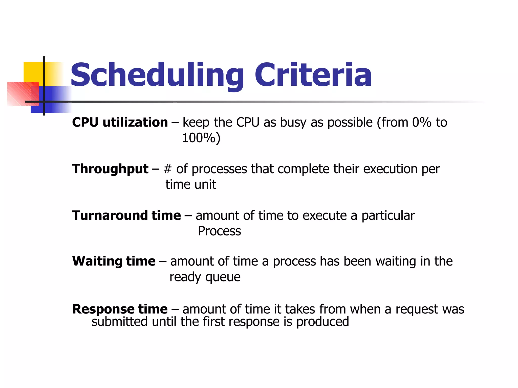
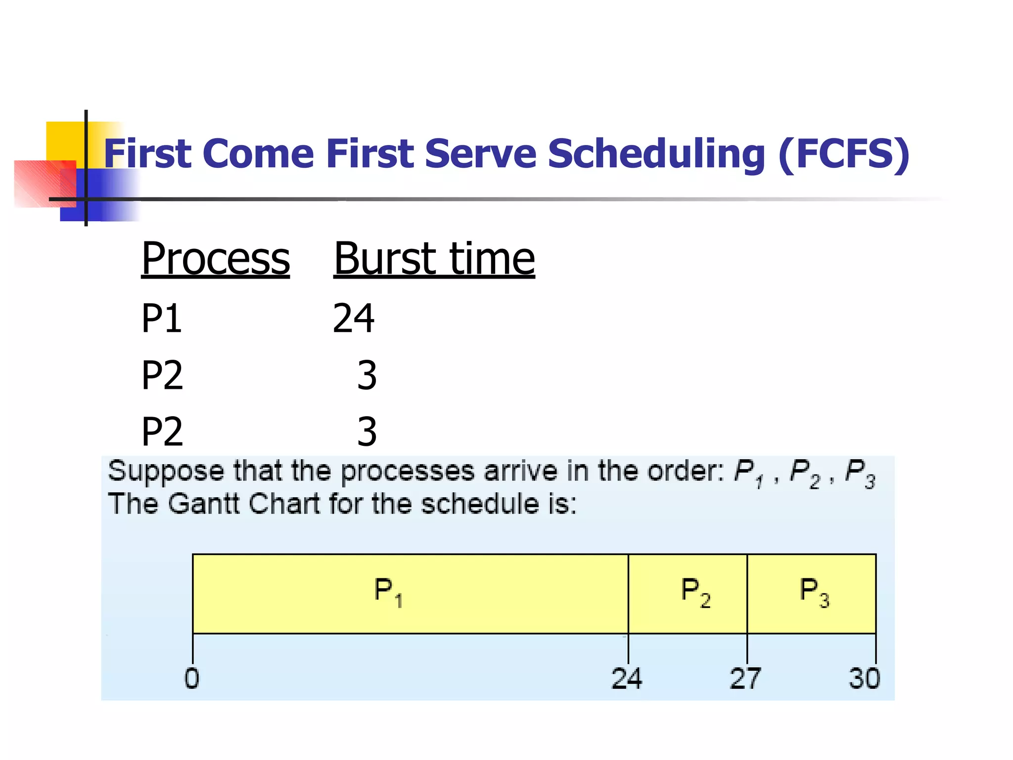
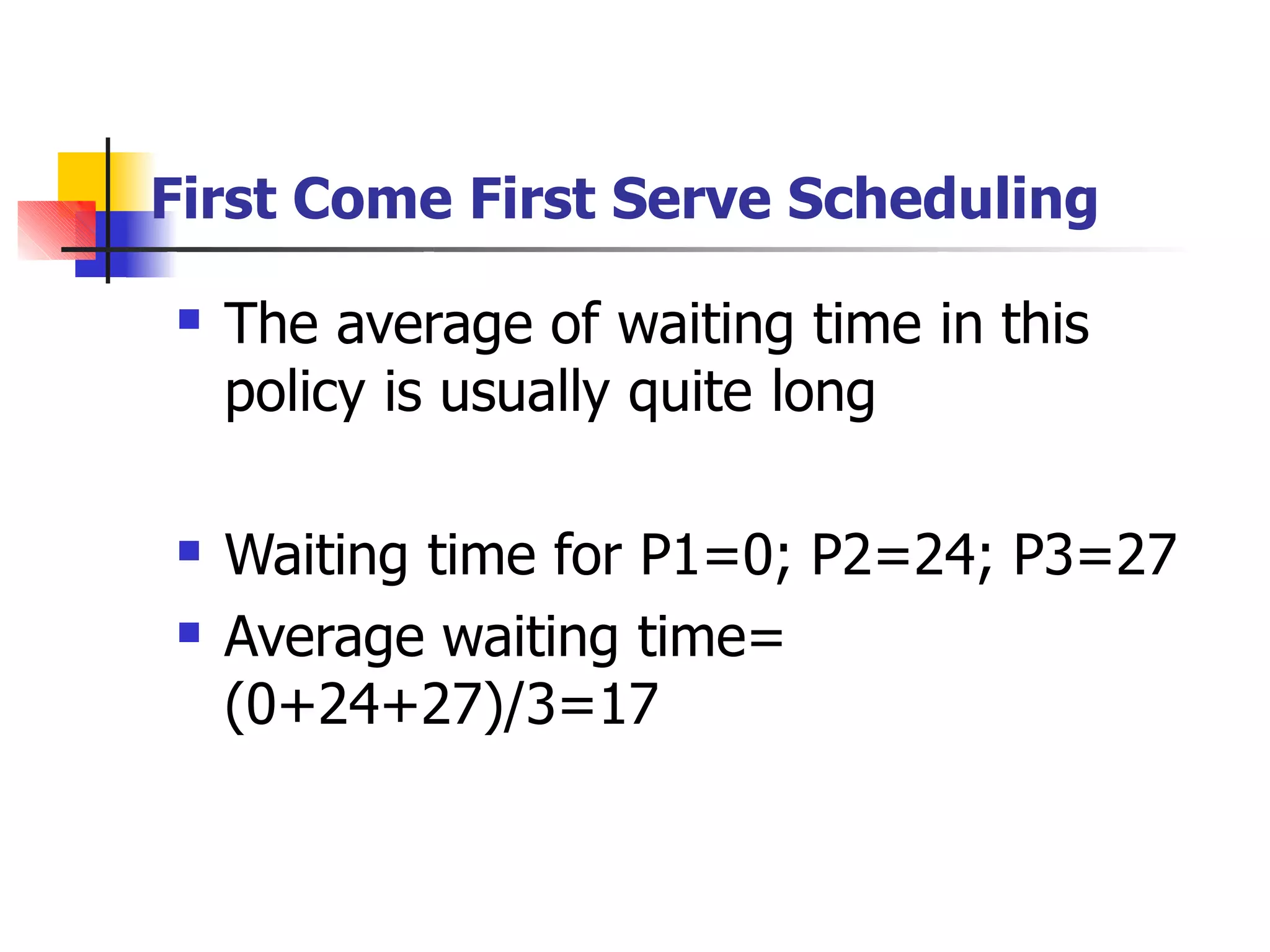
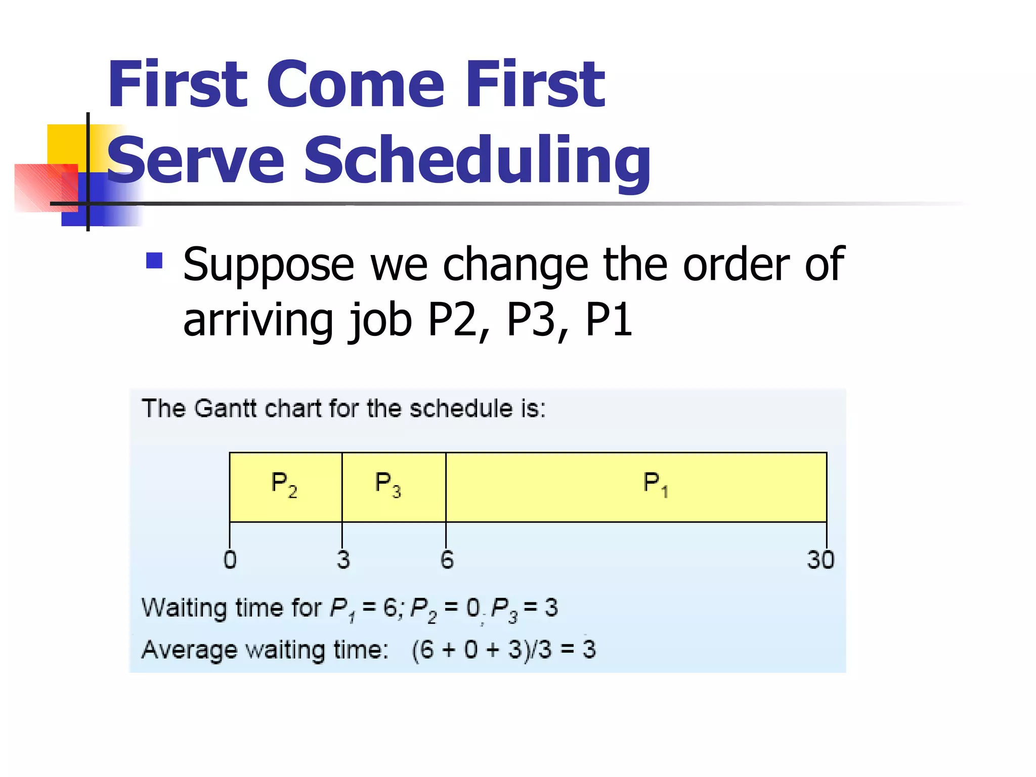
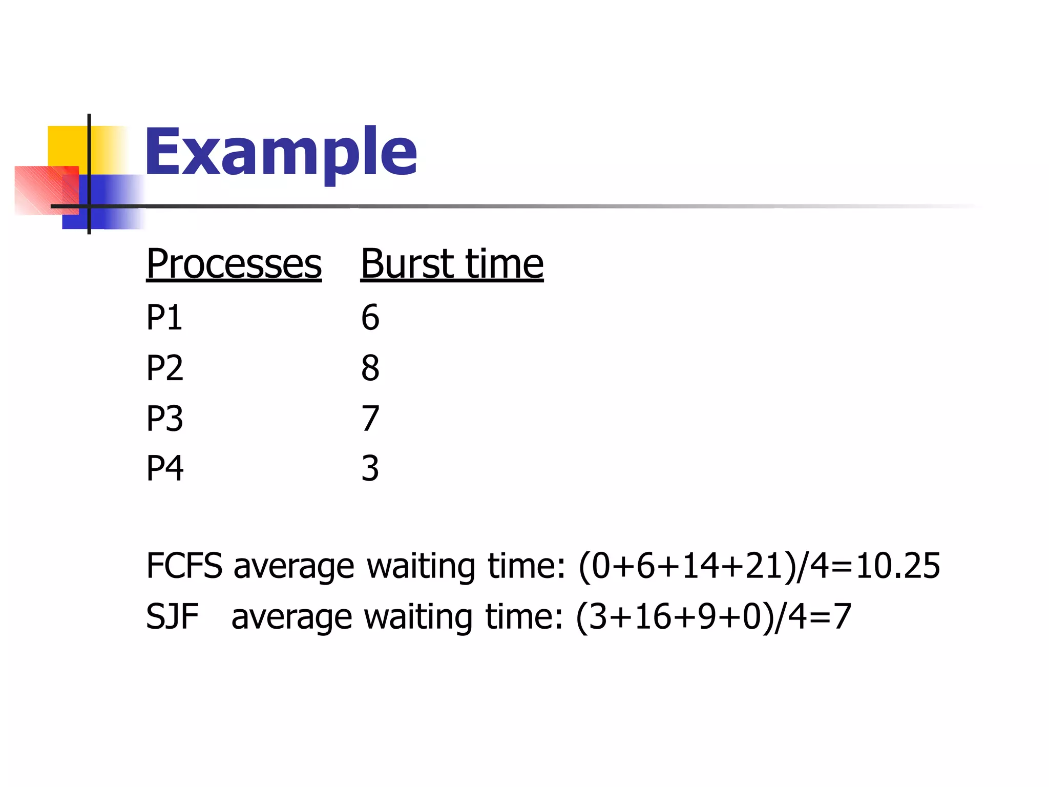
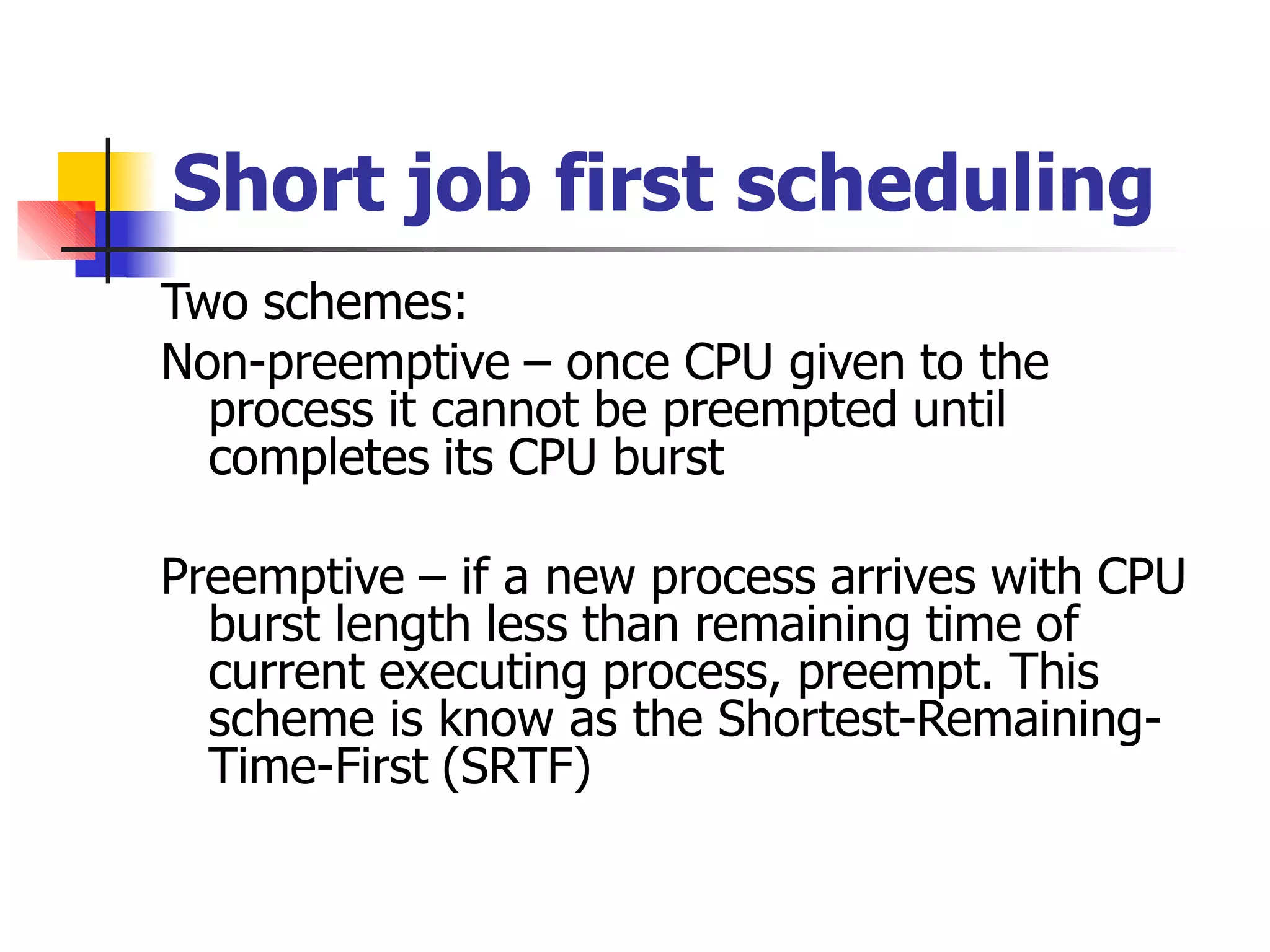
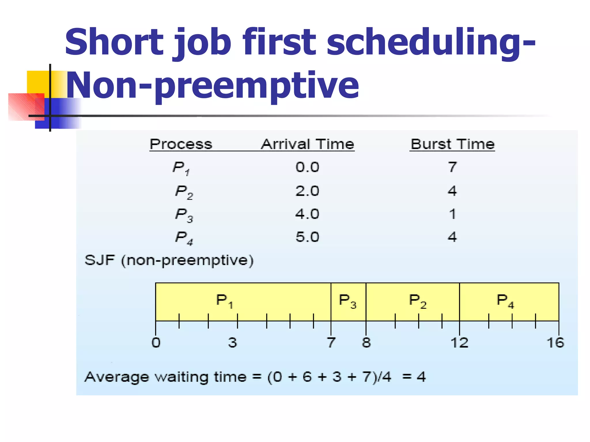
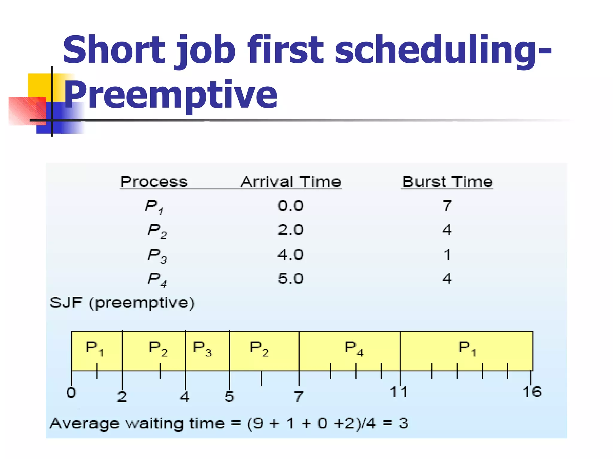
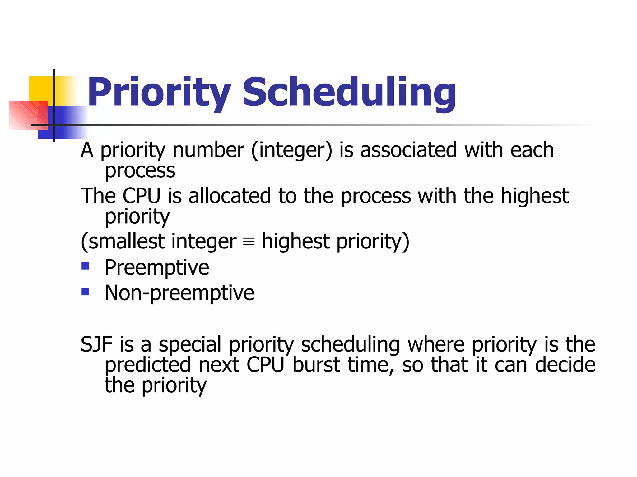
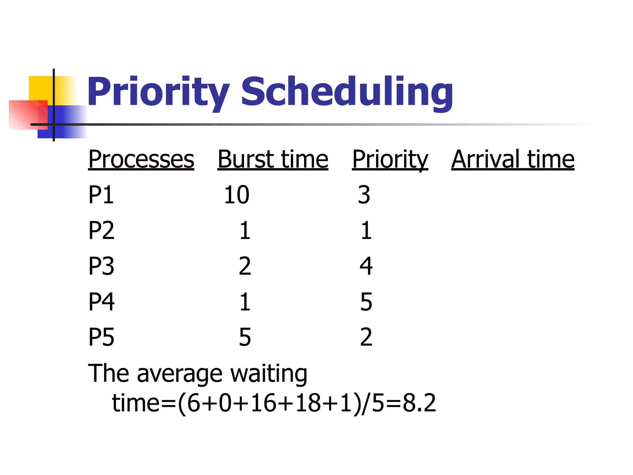
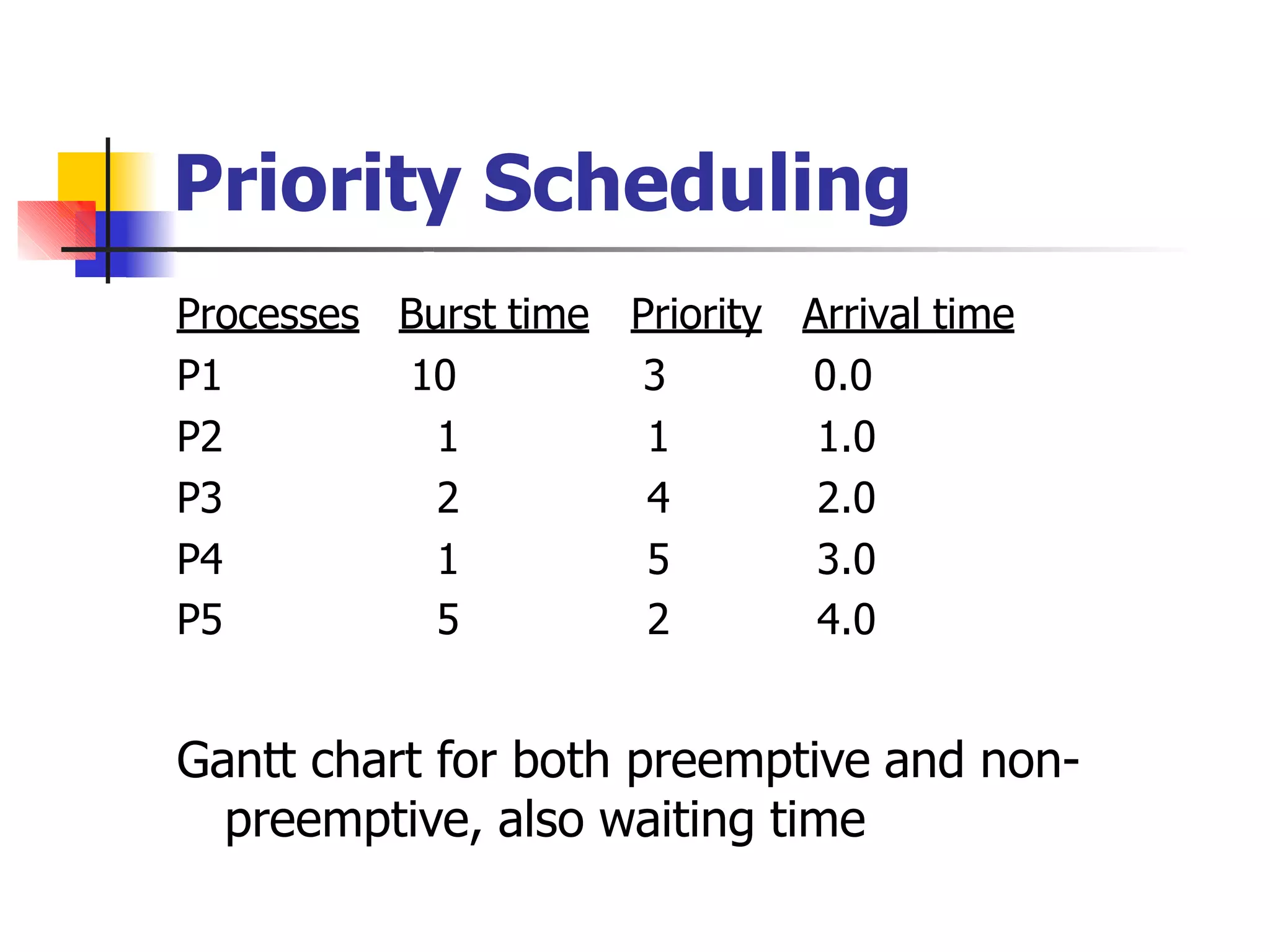
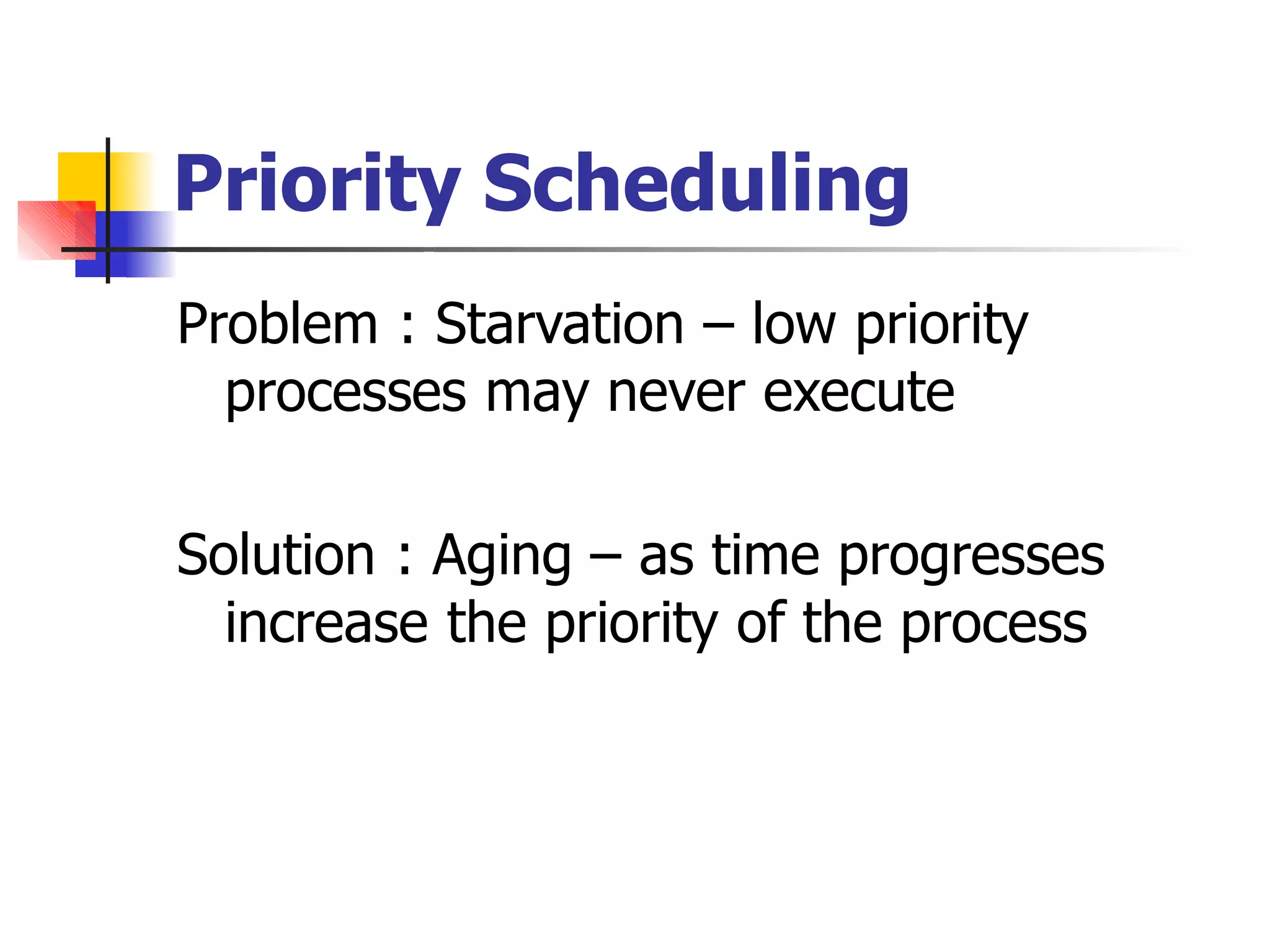
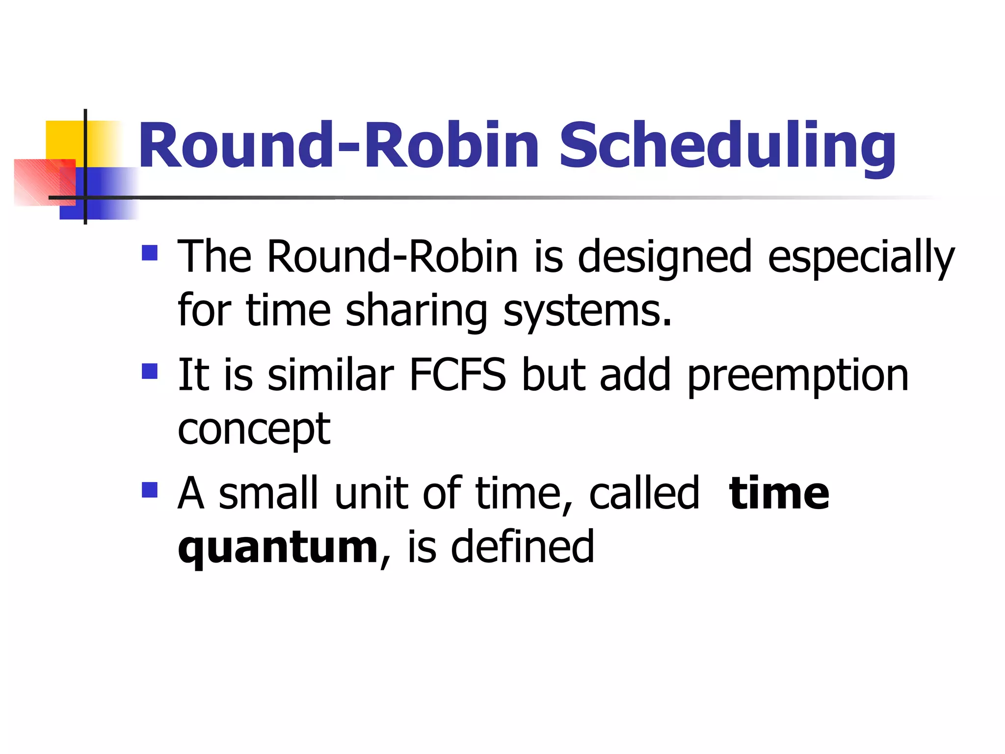
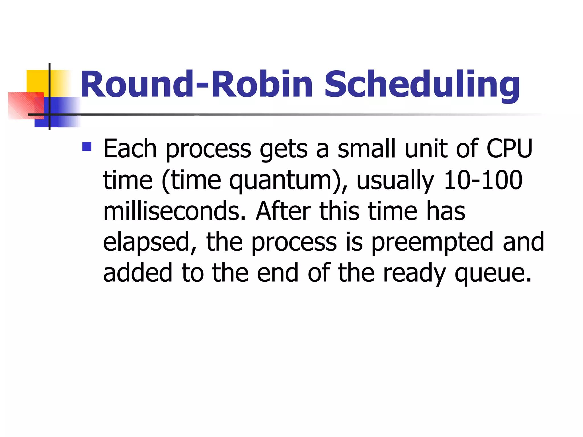
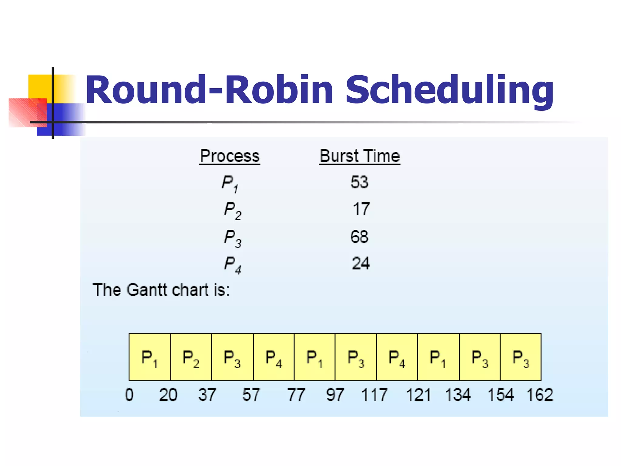
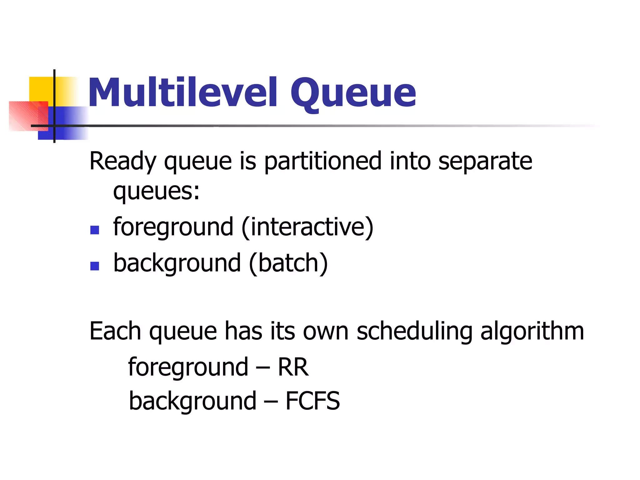
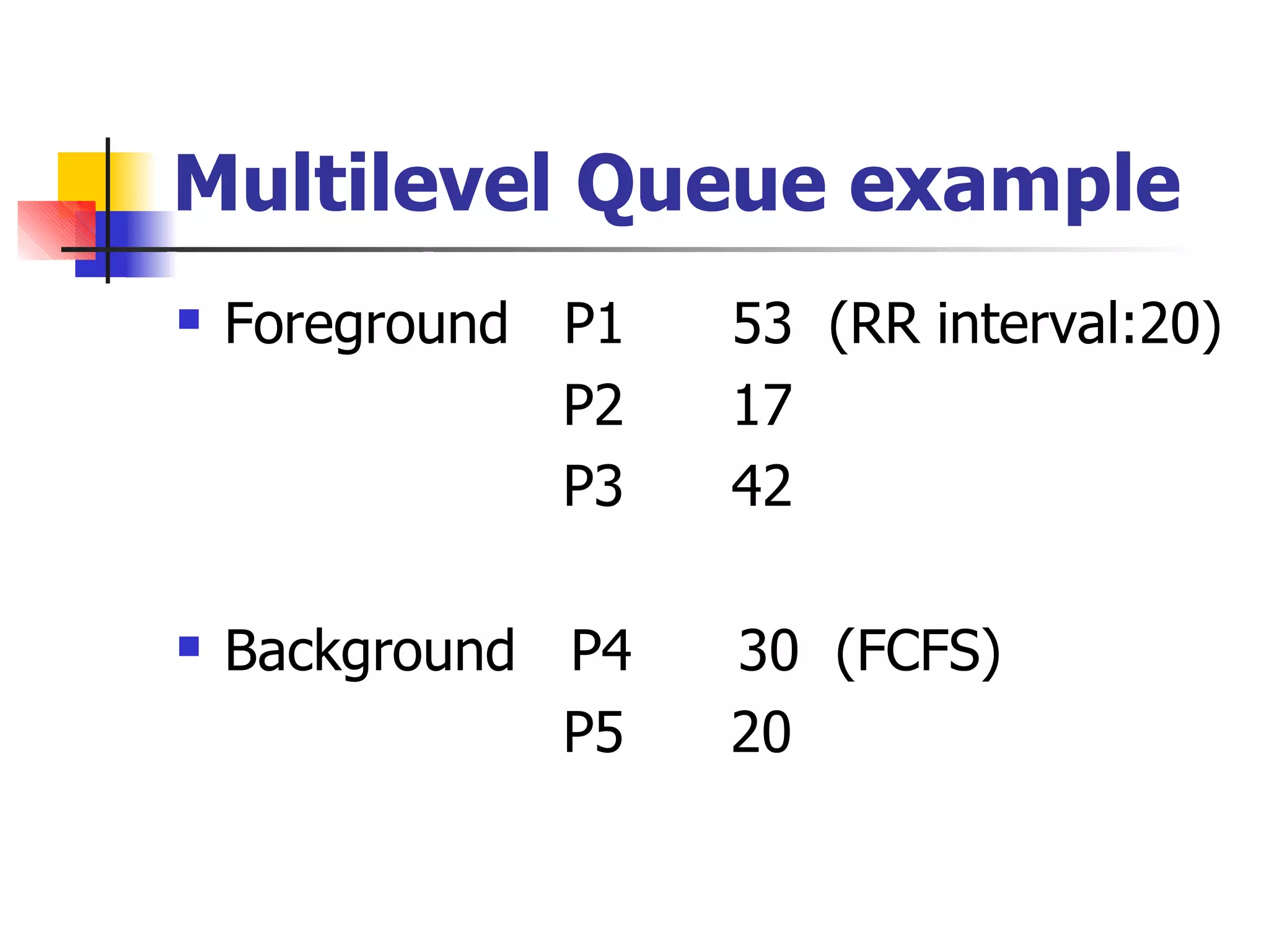
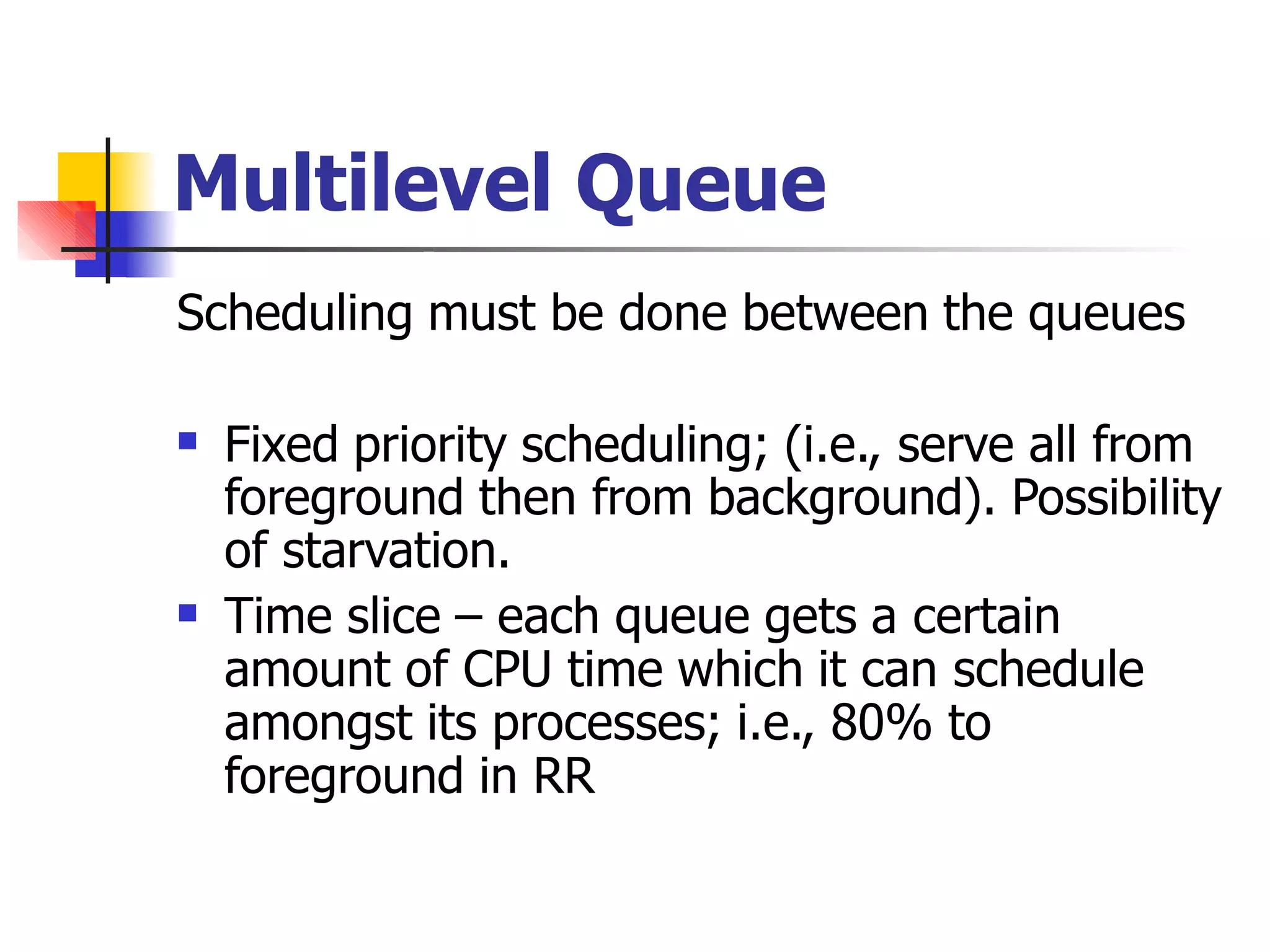
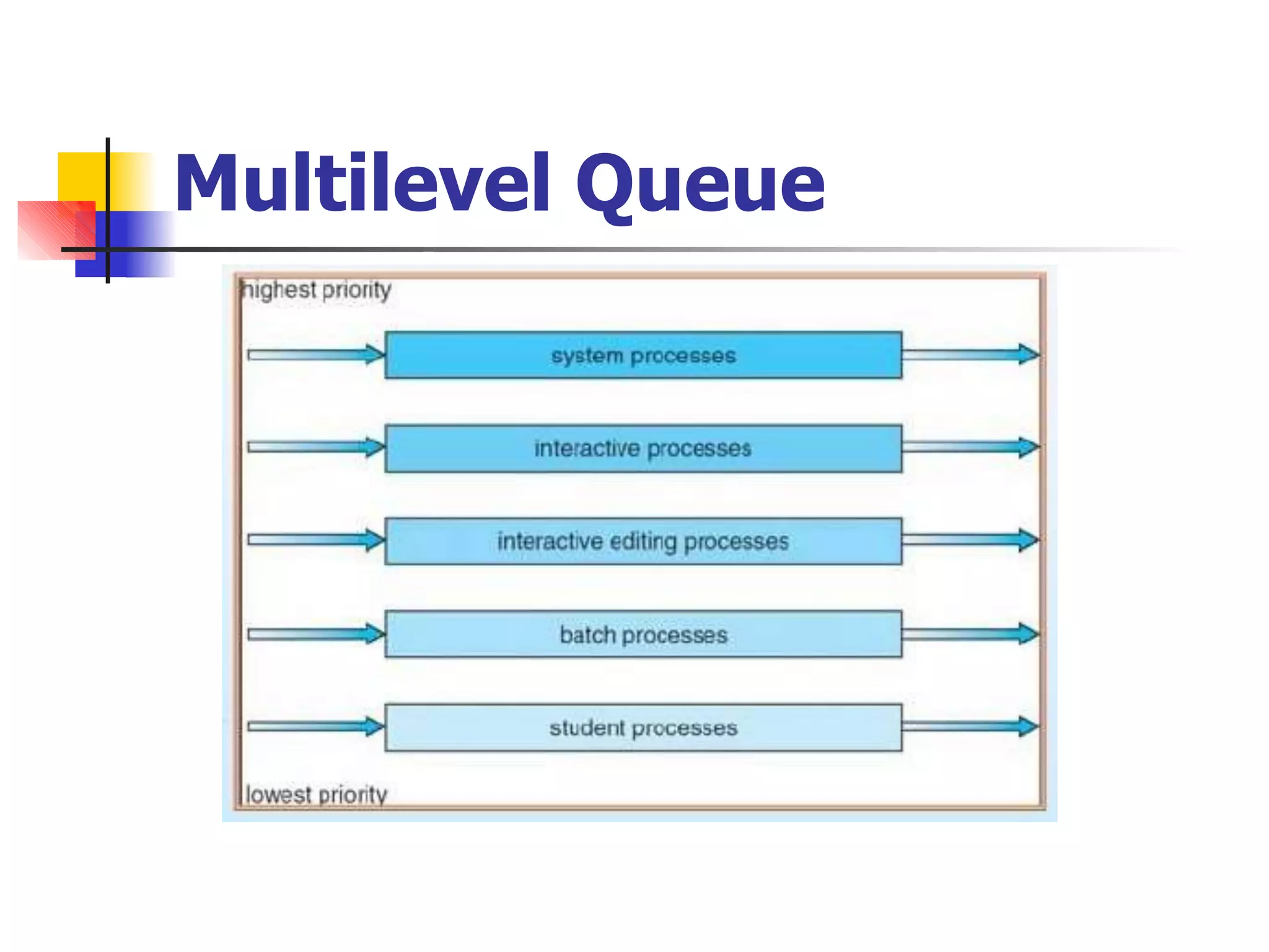
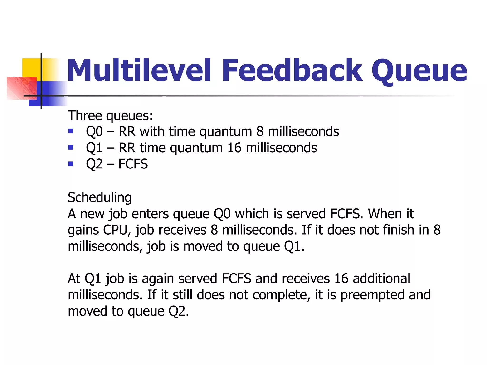
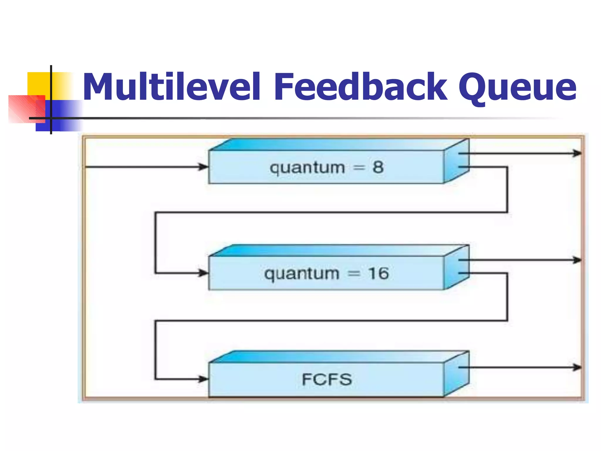
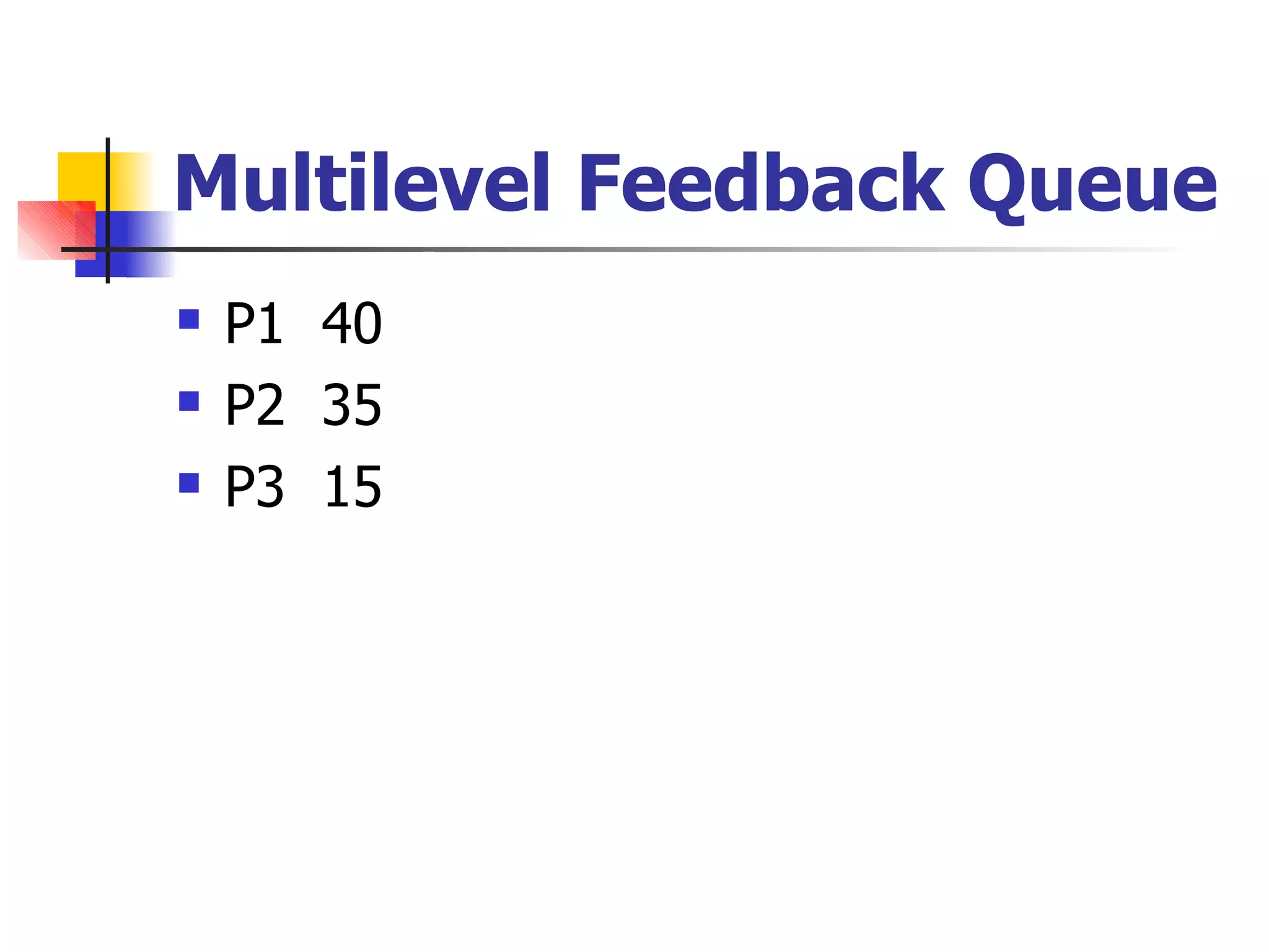
Shri Ramswaroop Memorial
University
NAME – VAIBHAV SAHU
ROLL NO. – 202110101110079
COURSE – B.TECH CS-43
SUBJECT – OPERATING SYSTEMS
SUBJECT CODE- BCS4022
SESSION – 2023-24
SUBMITTED TO - NEERAJ KUMAR SIR
SUBMITTED BY- VAIBHAV SAHU
Scheduling Criteria
CPU utilization – keep the CPU as busy as possible (from 0% to
100%)
Throughput – # of processes that complete their execution per
time unit
Turnaround time – amount of time to execute a particular
Process
Waiting time – amount of time a process has been waiting in the
ready queue
Response time – amount of time it takes from when a request was
submitted until the first response is produced
Optimization Criteria
 Max CPU utilization
Max throughput
Min turnaround time
Min waiting time
Min Response time




Scheduling Algorithems
 First Come First Serve Scheduling
Shortest Job First Scheduling
Priority Scheduling
Round-Robin Scheduling
Multilevel Queue Scheduling
Multilevel Feedback-Queue
Scheduling





First Come First Serve Scheduling (FCFS)
Process Burst time
P1 24
P2 3
P2 3
First Come First Serve Scheduling
 The average of waiting time in this
policy is usually quite long
 Waiting time for P1=0; P2=24; P3=27
Average waiting time=
(0+24+27)/3=17

First Come First
Serve Scheduling
 Suppose we change the order of
arriving job P2, P3, P1
First Come First
Serve Scheduling
 Consider if we have a CPU-bound process and
many I/O-bound processes
 There is a convoy effect as all the other
processes waiting for one of the big process
to get off the CPU
 FCFS scheduling algorithm is non-preemptive
Short job first scheduling (SJF)
 This algorithm associates with each
process the length of the processes’
next CPU burst
 If there is a tie, FCFS is used
In other words, this algorithm can be
also regard as shortest-next-cpu-burst
algorithm

Short job first scheduling
 SJF is optimal – gives minimum average
waiting time for a given set of
processes
Example
Processes Burst time
P1 6
P2 8
P3 7
P4 3
FCFS average waiting time: (0+6+14+21)/4=10.25
SJF average waiting time: (3+16+9+0)/4=7
Short job first scheduling
Two schemes:
Non-preemptive – once CPU given to the
process it cannot be preempted until
completes its CPU burst
Preemptive – if a new process arrives with CPU
burst length less than remaining time of
current executing process, preempt. This
scheme is know as the Shortest-Remaining-
Time-First (SRTF)
Short job first scheduling-
Non-preemptive
Short job first scheduling-
Preemptive
Priority Scheduling
A priority number (integer) is associated with each
process
The CPU is allocated to the process with the highest
priority
(smallest integer ≡ highest priority)


Preemptive
Non-preemptive
SJF is a special priority scheduling where priority is the
predicted next CPU burst time, so that it can decide
the priority
Priority Scheduling
Processes Burst time Priority Arrival time
P1 10 3
P2 1 1
P3 2 4
P4 1 5
P5 5 2
The average waiting
time=(6+0+16+18+1)/5=8.2
Priority Scheduling
Processes Burst time Priority Arrival time
P1 10 3 0.0
P2 1 1 1.0
P3 2 4 2.0
P4 1 5 3.0
P5 5 2 4.0
Gantt chart for both preemptive and non-
preemptive, also waiting time
Priority Scheduling
Problem : Starvation – low priority
processes may never execute
Solution : Aging – as time progresses
increase the priority of the process
Round-Robin Scheduling
 The Round-Robin is designed especially
for time sharing systems.
It is similar FCFS but add preemption
concept
A small unit of time, called time
quantum, is defined


Round-Robin Scheduling
 Each process gets a small unit of CPU
time (time quantum), usually 10-100
milliseconds. After this time has
elapsed, the process is preempted and
added to the end of the ready queue.
Round-Robin Scheduling
 If there are n processes in the ready
queue and the time quantum is q, then
each process gets 1/n of the CPU time
in chunks of at most q time units at
once. No process waits more than
(n-1)q time units.
Round-Robin Scheduling
Performance
 q large => FIFO
 q small => q must be large with
respect to context switch, otherwise
overhead is too high
 Typically, higher average turnaround
than SJF, but better response
Round-Robin Scheduling
Multilevel Queue
Ready queue is partitioned into separate
queues:
 foreground (interactive)
 background (batch)
Each queue has its own scheduling algorithm
foreground – RR
background – FCFS
Multilevel Queue example
 Foreground P1 53 (RR interval:20)
P2 17
P3 42
 Background P4 30 (FCFS)
P5 20
Multilevel Queue
Scheduling must be done between the queues
 Fixed priority scheduling; (i.e., serve all from
foreground then from background). Possibility
of starvation.
Time slice – each queue gets a certain
amount of CPU time which it can schedule
amongst its processes; i.e., 80% to
foreground in RR

Multilevel Queue
Multilevel Feedback Queue
Three queues:



Q0 – RR with time quantum 8 milliseconds
Q1 – RR time quantum 16 milliseconds
Q2 – FCFS
Scheduling
A new job enters queue Q0 which is served FCFS. When it
gains CPU, job receives 8 milliseconds. If it does not finish in 8
milliseconds, job is moved to queue Q1.
At Q1 job is again served FCFS and receives 16 additional
milliseconds. If it still does not complete, it is preempted and
moved to queue Q2.
Multilevel Feedback Queue
 P1 40
P2 35
P3 15



csc4320chapter5-2-101203002830-phpapp01.pdf

  • 1.
    Shri Ramswaroop Memorial University NAME– VAIBHAV SAHU ROLL NO. – 202110101110079 COURSE – B.TECH CS-43 SUBJECT – OPERATING SYSTEMS SUBJECT CODE- BCS4022 SESSION – 2023-24 SUBMITTED TO - NEERAJ KUMAR SIR SUBMITTED BY- VAIBHAV SAHU
  • 2.
    Scheduling Criteria CPU utilization– keep the CPU as busy as possible (from 0% to 100%) Throughput – # of processes that complete their execution per time unit Turnaround time – amount of time to execute a particular Process Waiting time – amount of time a process has been waiting in the ready queue Response time – amount of time it takes from when a request was submitted until the first response is produced
  • 3.
    Optimization Criteria  MaxCPU utilization Max throughput Min turnaround time Min waiting time Min Response time    
  • 4.
    Scheduling Algorithems  FirstCome First Serve Scheduling Shortest Job First Scheduling Priority Scheduling Round-Robin Scheduling Multilevel Queue Scheduling Multilevel Feedback-Queue Scheduling     
  • 5.
    First Come FirstServe Scheduling (FCFS) Process Burst time P1 24 P2 3 P2 3
  • 6.
    First Come FirstServe Scheduling  The average of waiting time in this policy is usually quite long  Waiting time for P1=0; P2=24; P3=27 Average waiting time= (0+24+27)/3=17 
  • 7.
    First Come First ServeScheduling  Suppose we change the order of arriving job P2, P3, P1
  • 8.
    First Come First ServeScheduling  Consider if we have a CPU-bound process and many I/O-bound processes  There is a convoy effect as all the other processes waiting for one of the big process to get off the CPU  FCFS scheduling algorithm is non-preemptive
  • 9.
    Short job firstscheduling (SJF)  This algorithm associates with each process the length of the processes’ next CPU burst  If there is a tie, FCFS is used In other words, this algorithm can be also regard as shortest-next-cpu-burst algorithm 
  • 10.
    Short job firstscheduling  SJF is optimal – gives minimum average waiting time for a given set of processes
  • 11.
    Example Processes Burst time P16 P2 8 P3 7 P4 3 FCFS average waiting time: (0+6+14+21)/4=10.25 SJF average waiting time: (3+16+9+0)/4=7
  • 12.
    Short job firstscheduling Two schemes: Non-preemptive – once CPU given to the process it cannot be preempted until completes its CPU burst Preemptive – if a new process arrives with CPU burst length less than remaining time of current executing process, preempt. This scheme is know as the Shortest-Remaining- Time-First (SRTF)
  • 13.
    Short job firstscheduling- Non-preemptive
  • 14.
    Short job firstscheduling- Preemptive
  • 15.
    Priority Scheduling A prioritynumber (integer) is associated with each process The CPU is allocated to the process with the highest priority (smallest integer ≡ highest priority)   Preemptive Non-preemptive SJF is a special priority scheduling where priority is the predicted next CPU burst time, so that it can decide the priority
  • 16.
    Priority Scheduling Processes Bursttime Priority Arrival time P1 10 3 P2 1 1 P3 2 4 P4 1 5 P5 5 2 The average waiting time=(6+0+16+18+1)/5=8.2
  • 17.
    Priority Scheduling Processes Bursttime Priority Arrival time P1 10 3 0.0 P2 1 1 1.0 P3 2 4 2.0 P4 1 5 3.0 P5 5 2 4.0 Gantt chart for both preemptive and non- preemptive, also waiting time
  • 18.
    Priority Scheduling Problem :Starvation – low priority processes may never execute Solution : Aging – as time progresses increase the priority of the process
  • 19.
    Round-Robin Scheduling  TheRound-Robin is designed especially for time sharing systems. It is similar FCFS but add preemption concept A small unit of time, called time quantum, is defined  
  • 20.
    Round-Robin Scheduling  Eachprocess gets a small unit of CPU time (time quantum), usually 10-100 milliseconds. After this time has elapsed, the process is preempted and added to the end of the ready queue.
  • 21.
  • 22.
    Round-Robin Scheduling  Ifthere are n processes in the ready queue and the time quantum is q, then each process gets 1/n of the CPU time in chunks of at most q time units at once. No process waits more than (n-1)q time units.
  • 23.
    Round-Robin Scheduling Performance  qlarge => FIFO  q small => q must be large with respect to context switch, otherwise overhead is too high  Typically, higher average turnaround than SJF, but better response
  • 24.
  • 25.
    Multilevel Queue Ready queueis partitioned into separate queues:  foreground (interactive)  background (batch) Each queue has its own scheduling algorithm foreground – RR background – FCFS
  • 26.
    Multilevel Queue example Foreground P1 53 (RR interval:20) P2 17 P3 42  Background P4 30 (FCFS) P5 20
  • 27.
    Multilevel Queue Scheduling mustbe done between the queues  Fixed priority scheduling; (i.e., serve all from foreground then from background). Possibility of starvation. Time slice – each queue gets a certain amount of CPU time which it can schedule amongst its processes; i.e., 80% to foreground in RR 
  • 28.
  • 29.
    Multilevel Feedback Queue Threequeues:    Q0 – RR with time quantum 8 milliseconds Q1 – RR time quantum 16 milliseconds Q2 – FCFS Scheduling A new job enters queue Q0 which is served FCFS. When it gains CPU, job receives 8 milliseconds. If it does not finish in 8 milliseconds, job is moved to queue Q1. At Q1 job is again served FCFS and receives 16 additional milliseconds. If it still does not complete, it is preempted and moved to queue Q2.
  • 30.
  • 31.
    Multilevel Feedback Queue P1 40 P2 35 P3 15  