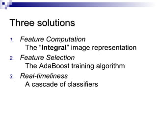
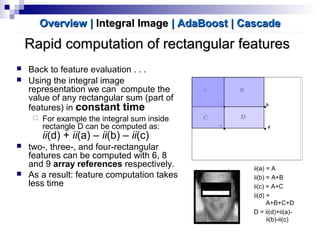
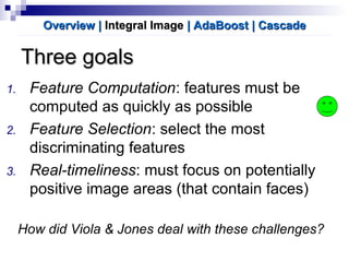
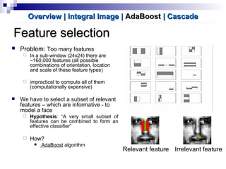
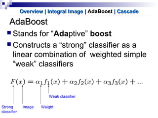
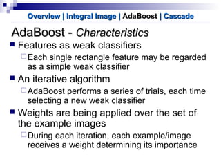
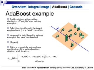
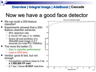
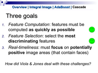
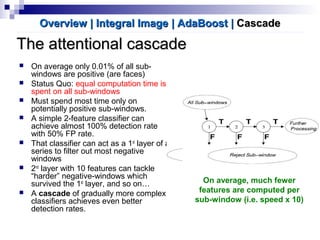
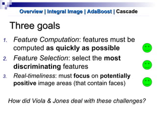
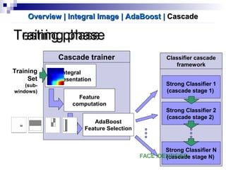
Robust Real Time Face Detection

Robust Real-time FaceRobust Real-time Face
DetectionDetection
byby
Paul Viola and Michael Jones, 2002Paul Viola and Michael Jones, 2002
Presentation by Kostantina Palla & Alfredo Kalaitzis
School of Informatics
University of Edinburgh
February 20, 2009

OverviewOverview
 Robust – very high Detection Rate (True-Positive
Rate) & very low False-Positive Rate… always.
 Real Time – For practical applications at least 2
frames per second must be processed.
 Face Detection – not recognition. The goal is to
distinguish faces from non-faces (face detection is the
first step in the identification process)

Three goals & a conlcusionThree goals & a conlcusion
1. Feature Computation: what features? And how
can they be computed as quickly as possible
2. Feature Selection: select the most
discriminating features
3. Real-timeliness: must focus on potentially
positive areas (that contain faces)
4. Conclusion: presentation of results and
discussion of detection issues.
How did Viola & Jones deal with these challenges?

1. Feature Computation
The “Integral” image representation
2. Feature Selection
The AdaBoost training algorithm
3. Real-timeliness
A cascade of classifiers
Three solutionsThree solutions

FeaturesFeatures
 Can a simple feature (i.e. a value) indicate
the existence of a face?
 All faces share some similar properties
 The eyes region is darker than the
upper-cheeks.
 The nose bridge region is brighter than
the eyes.
 That is useful domain knowledge
 Need for encoding of Domain Knowledge:
 Location - Size: eyes & nose bridge
region
 Value: darker / brighter
OverviewOverview || Integral ImageIntegral Image | AdaBoost| AdaBoost | Cascade| Cascade

Rectangle featuresRectangle features
 Rectangle features:
 Value = ∑ (pixels in black area) - ∑
(pixels in white area)
 Three types: two-, three-, four-rectangles,
Viola&Jones used two-rectangle features
 For example: the difference in brightness
between the white &black rectangles over
a specific area
 Each feature is related to a special
location in the sub-window
 Each feature may have any size
 Why not pixels instead of features?
 Features encode domain knowledge
 Feature based systems operate faster
Overview |Overview | Integral ImageIntegral Image | AdaBoost| AdaBoost | Cascade| Cascade

Integral Image RepresentationIntegral Image Representation
(also check back-up slide #1)(also check back-up slide #1)
 Given a detection resolution of
24x24 (smallest sub-window), the set
of different rectangle features is
~160,000 !
 Need for speed
 Introducing Integral Image
Representation
 Definition: The integral image at
location (x,y), is the sum of the
pixels above and to the left of
(x,y), inclusive
 The Integral image can be computed
in a single pass and only once for
each sub-window!
( ) ( )
( ) ( ) ( )
( ) ( ) ( )
' , '
formal definition:
, ', '
Recursive definition:
, , 1 ,
, 1, ,
x x y y
ii x y i x y
s x y s x y i x y
ii x y ii x y s x y
≤ ≤
=
= − +
= − +
∑
y
x

back-up slide #1back-up slide #1
0 1 1 1
1 2 2 3
1 2 1 1
1 3 1 0
IMAGE
0 1 2 3
1 4 7 11
2 7 11 16
3 11 16 21
INTEGRAL IMAGE

Rapid computation of rectangular featuresRapid computation of rectangular features
 Back to feature evaluation . . .
 Using the integral image
representation we can compute the
value of any rectangular sum (part of
features) in constant time
 For example the integral sum inside
rectangle D can be computed as:
ii(d) + ii(a) – ii(b) – ii(c)
 two-, three-, and four-rectangular
features can be computed with 6, 8
and 9 array references respectively.
 As a result: feature computation takes
less time
ii(a) = A
ii(b) = A+B
ii(c) = A+C
ii(d) =
A+B+C+D
D = ii(d)+ii(a)-
ii(b)-ii(c)

Three goalsThree goals
1. Feature Computation: features must be
computed as quickly as possible
positive image areas (that contain faces)

Feature selectionFeature selection
 Problem: Too many features
 In a sub-window (24x24) there are
~160,000 features (all possible
combinations of orientation, location
and scale of these feature types)
 impractical to compute all of them
(computationally expensive)
 We have to select a subset of relevant
features – which are informative - to
model a face
 Hypothesis: “A very small subset of
features can be combined to form an
effective classifier”
 How?
 AdaBoost algorithm
Overview | Integral ImageOverview | Integral Image || AdaBoostAdaBoost | Cascade| Cascade
Relevant feature Irrelevant feature

AdaBoostAdaBoost
 Stands for “Adaptive” boost
 Constructs a “strong” classifier as a
linear combination of weighted simple
“weak” classifiers
Strong
classifier
Weak classifier
WeightImage

AdaBoost -AdaBoost - CharacteristicsCharacteristics
 Features as weak classifiers
Each single rectangle feature may be regarded
as a simple weak classifier
 An iterative algorithm
AdaBoost performs a series of trials, each time
selecting a new weak classifier
 Weights are being applied over the set of
the example images
During each iteration, each example/image
receives a weight determining its importance

AdaBoost -AdaBoost - Getting the idea…Getting the idea…
 Given: example images labeled +/-
 Initially, all weights set equally
 Repeat T times
 Step 1: choose the most efficient weak classifier that will be a
component of the final strong classifier (Problem! Remember the huge
number of features…)
 Step 2: Update the weights to emphasize the examples which were
incorrectly classified
 This makes the next weak classifier to focus on “harder” examples
 Final (strong) classifier is a weighted combination of the T “weak” classifiers
 Weighted according to their accuracy




≥
= ∑ ∑= =
otherwise
x
xh
T
t
T
t ttt h
0
2
1
)(1
)( 1 1αα
(pseudo-code at back-up slide #2)(pseudo-code at back-up slide #2)

AdaBoost –AdaBoost – Feature SelectionFeature Selection
Problem
 On each round, large set of possible weak classifiers (each simple
classifier consists of a single feature) – Which one to choose?
 choose the most efficient (the one that best separates the
examples – the lowest error)
 choice of a classifier corresponds to choice of a feature
 At the end, the ‘strong’ classifier consists of T features
Conclusion
 AdaBoost searches for a small number of good classifiers – features
(feature selection)
 adaptively constructs a final strong classifier taking into account the
failures of each one of the chosen weak classifiers (weight appliance)
 AdaBoost is used to both select a small set of features and train a
strong classifier

 AdaBoost starts with a uniform
distribution of “weights” over training
examples.
 Select the classifier with the lowest
weighted error (i.e. a “weak” classifier)
 Increase the weights on the training
examples that were misclassified.
 (Repeat)
 At the end, carefully make a linear
combination of the weak classifiers
obtained at all iterations.
AdaBoost exampleAdaBoost example
( )1 1 1
strong
1
1 ( ) ( )
( ) 2
0 otherwise
n n nh h
h

α + + α ≥ α + + α
= 

x x
x
K K
Slide taken from a presentation by Qing Chen, Discover Lab, University of Ottawa

Now we have a good face detectorNow we have a good face detector
 We can build a 200-feature
classifier!
 Experiments showed that a 200-
feature classifier achieves:
 95% detection rate
 0.14x10-3
FP rate (1 in 14084)
 Scans all sub-windows of a
384x288 pixel image in 0.7
seconds (on Intel PIII 700MHz)
 The more the better (?)
 Gain in classifier performance
 Lose in CPU time
 Verdict: good & fast, but not
enough
 Competitors achieve close to 1 in
a 1.000.000 FP rate!
 0.7 sec / frame IS NOT real-time.
Overview | Integral ImageOverview | Integral Image | AdaBoost| AdaBoost || CascadeCascade

Three goalsThree goals
1. Feature Computation: features must be
computed as quickly as possible
positive image areas (that contain faces)

The attentional cascadeThe attentional cascade
 On average only 0.01% of all sub-
windows are positive (are faces)
 Status Quo: equal computation time is
spent on all sub-windows
 Must spend most time only on
potentially positive sub-windows.
 A simple 2-feature classifier can
achieve almost 100% detection rate
with 50% FP rate.
 That classifier can act as a 1st
layer of a
series to filter out most negative
windows
 2nd
layer with 10 features can tackle
“harder” negative-windows which
survived the 1st
layer, and so on…
 A cascade of gradually more complex
classifiers achieves even better
detection rates.
On average, much fewer
features are computed per
sub-window (i.e. speed x 10)

Training a cascade of classifiersTraining a cascade of classifiers
Strong classifier definition:
,
where ,
 Keep in mind:
 Competitors achieved 95% TP rate,10-6
FP rate
 These are the goals. Final cascade must do better!
 Given the goals, to design a cascade we must choose:
 Number of layers in cascade (strong classifiers)
 Number of features of each strong classifier (the ‘T’ in definition)
 Threshold of each strong classifier (the in definition)
 Optimization problem:
 Can we find optimum combination?
∑=
T
t t1
2
1
α
TREMENDOUSLY
DIFFICULT
PROBLEM

A simple framework for cascade trainingA simple framework for cascade training
 Do not despair. Viola & Jones suggested a heuristic algorithm for
the cascade training: (pseudo-code at backup slide # 3)
 does not guarantee optimality
 but produces a “effective” cascade that meets previous goals
 Manual Tweaking:
 overall training outcome is highly depended on user’s choices
 select fi (Maximum Acceptable False Positive rate / layer)
 select di (Minimum Acceptable True Positive rate / layer)
 select Ftarget (Target Overall FP rate)
 possible repeat trial & error process for a given training set
 Until Ftarget is met:
 Add new layer:
 Until fi , di rates are met for this layer
 Increase feature number & train new strong classifier with AdaBoost
 Determine rates of layer on validation set

backup slide #3backup slide #3
• User selects values for f, the maximum acceptable false positive rate per layer and d,
the minimum acceptable detection rate per layer.
• User selects target overall false positive rate Ftarget.
• P = set of positive examples
• N = set of negative examples
• F0 = 1.0; D0 = 1.0; i = 0
While Fi > Ftarget
i++
ni = 0; Fi = Fi-1
while Fi > f x Fi-1
oni ++
oUse P and N to train a classifier with ni features using AdaBoost
oEvaluate current cascaded classifier on validation set to determine Fi and Di
oDecrease threshold for the ith classifier until the current cascaded classifier has
a detection rate of at least d x Di-1 (this also affects Fi)
N = ∅
If Fi > Ftarget then evaluate the current cascaded detector on the set of non-face
images and put any false detections into the set N.

Training
Set
(sub-
windows)
Integral
Representation
Feature
computation
AdaBoost
Feature Selection
Cascade trainer
Testing phaseTesting phaseTraining phaseTraining phase
Strong Classifier 1
(cascade stage 1)
Strong Classifier N
(cascade stage N)
Classifier cascade
framework
Strong Classifier 2
(cascade stage 2)
FACE IDENTIFIED

pros …pros …
 Extremely fast feature computation
 Efficient feature selection
 Scale and location invariant detector
 Instead of scaling the image itself (e.g. pyramid-filters), we scale the
features.
 Such a generic detection scheme can be trained for detection of
other types of objects (e.g. cars, hands)
…… and consand cons
 Detector is most effective only on frontal images of faces
 can hardly cope with 45o
face rotation
 Sensitive to lighting conditions
 We might get multiple detections of the same face, due to
overlapping sub-windows.

ResultsResults
(detailed results at back-up slide #4)(detailed results at back-up slide #4)

Results (Cont.)Results (Cont.)

 Viola & Jones prepared their final Detector cascade:
 38 layers, 6060 total features included
 1st
classifier- layer, 2-features
 50% FP rate, 99.9% TP rate
 2nd
classifier- layer, 10-features
 20% FP rate, 99.9% TP rate
 next 2 layers 25-features each, next 3 layers 50-features each
 and so on…
 Tested on the MIT+MCU test set
 a 384x288 pixel image on an PC (dated 2001) took about 0.067
seconds
Detector 10 31 50 65 78 95 167 422
Viola-Jones 76.1% 88.4% 91.4% 92.0% 92.1% 92.9% 93.9% 94.1%
Rowley-Baluja-Kanade 83.2% 86.0% - - 89.2% 89.2% 90.1% 89.9%
Schneiderman-Kanade - - - 94.4% - - - -
Roth-Yang-Ajuha - - - - - - - -
False detections
Detection rates for various numbers of false positives on the MIT+MCU test set containing 130
images and 507 faces (Viola & Jones 2002)
backup slide #4backup slide #4

Thank you for listening!Thank you for listening!

Robust Real Time Face Detection

More Related Content

Similar to Robust Real Time Face Detection

More from Syed Zaid Irshad

Recently uploaded

Robust Real Time Face Detection

Editor's Notes