ROBOTICS-LATEST-PPT.pdf

Introduction to Robotics
We will be studying Industrial manipulator
type Robots.
3

• Introduction to Robotics
• Classification of Robots
• Robot coordinates
• Work volumes and Reference Frames
• Robot Applications.
4

Automation vs. robots
• Automation –Machinery designed to carry out a specific task
– Bottling machine
– Dishwasher
– Paint sprayer
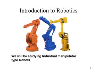
• Robots – machinery designed
to carry out a variety of tasks
– Pick and place arms
– Mobile robots
– Computer Numerical Control
machines
(These are always better
than robots, because they
can be optimally designed
for a particular task).
5

“Robot” coined by Karel Capek in a 1921 science-fiction Czech play
6

Robotics Terminology
7
Robot - Mechanical device that performs
human tasks, either automatically or by
remote control.
Robotics - Study and application of robot
technology.
Telerobotics - Robot that is operated
remotely.

Laws of Robotics
8
 Asimov proposed three “Laws of Robotics”
 Law 1: A robot may not injure a human being or
through inaction, allow a human being to come to
harm.
 Law 2: A robot must obey orders given to it by
human beings, except where such orders would
conflict with the first law.
 Law 3: A robot must protect its own existence as long
as such protection does not conflict with the first law.

Ideal Tasks
Tasks which are:
– Dangerous
• Space exploration
• chemical spill cleanup
• disarming bombs
• disaster cleanup
– Boring and/or repetitive
• Welding car frames
• part pick and place
• manufacturing parts.
– High precision or high speed
• Electronics testing
• Surgery
• precision machining.
9

Robotics Timeline
• 1922 Czech author Karel Capek wrote a story called
Rossum’s Universal Robots and introduced the word
“Rabota”(meaning worker)
• 1954 George Devol developed the first programmable
Robot.
• 1955 Denavit and Hartenberg developed the
homogenous transformation matrices
• 1962 Unimation was formed, first industrial Robots
appeared.
• 1973 Cincinnati Milacron introduced the T3 model robot,
which became very popular in industry.
• 1990 Cincinnati Milacron was acquired by ABB
10

ROBOT
• Defined by Robotics Industry Association
(RIA) as
– a re-programmable, multifunctional manipulator
designed to move material, parts, tools or
specialized devices through variable programmed
motion for a variety of tasks
• possess certain anthropomorphic
characteristics
– mechanical arm
– sensors to respond to input
– Intelligence to make decisions
11

Accessories
• Acutators : Actuators are the muscles of the
manipulators. Common types of actuators are
servomotors, stepper motors, pneumatic cylinders etc.
• Sensors : Sensors are used to collect information about
the internal state of the robot or to communicate with
the outside environment. Robots are often equipped
with external sensory devices such as a vision system,
touch and tactile sensors etc which help to
communicate with the environment
• Controller : The controller receives data from the
computer, controls the motions of the actuator and
coordinates these motions with the sensory feedback
information. 12

Robot Configurations
Some of the commonly used configurations in Robotics are
• Cartesian/Rectangular Gantry(3P) : These Robots are made of 3
Linear joints that orient the end effector, which are usually followed
by additional revolute joints.
13

Cartesian Robot - Work
Envelope
14

• Cylindrical (R2P): Cylindrical coordinate Robots have 2 prismatic
joints and one revolute joint.
15

Cylindrical Robot - Work
Envelope
16

• Spherical joint (2RP): They follow a spherical coordinate system,
which has one
17

Spherical Robot - Work
Envelope
18

• Articulated/anthropomorphic(3R) :An articulated robot’s joints are
all revolute, similar to a human’s arm.
19

• Selective Compliance Assembly Robot Arm (SCARA) (2R1P):
They have two revolute joints that are parallel and allow the Robot to
move in a horizontal plane, plus an additional prismatic joint that
moves vertically
20

Work Envelope concept
• Depending on the configuration and size of the
links and wrist joints, robots can reach a
collection of points called a Workspace.
• Alternately Workspace may be found empirically,
by moving each joint through its range of
motions and combining all space it can reach
and subtracting what space it cannot reach
22

Pure Spherical Jointed Arm - Work
envelope
23

WRIST
• typically has 3 degrees of freedom
– Roll involves rotating the wrist about the arm
axis
– Pitch up-down rotation of the wrist
– Yaw left-right rotation of the wrist
• End effector is mounted on the wrist
25

27
CONTROL METHODS
• Non Servo Control
– implemented by setting limits or mechanical
stops for each joint and sequencing the
actuation of each joint to accomplish the cycle
– end point robot, limited sequence robot, bang-
bang robot
– No control over the motion at the intermediate
points, only end points are known

• Programming accomplished by
– setting desired sequence of moves
– adjusting end stops for each axis accordingly
– the sequence of moves is controlled by a
“squencer”, which uses feedback received from
the end stops to index to next step in the program
• Low cost and easy to maintain, reliable
• relatively high speed
• repeatability of up to 0.01 inch
• limited flexibility
• typically hydraulic, pneumatic drives
28

• Servo Control
– Point to point Control
– Continuous Path Control
• Closed Loop control used to monitor
position, velocity (other variables) of
each joint
29

Point-to-Point Control
• Only the end points are programmed, the
path used to connect the end points are
computed by the controller
• user can control velocity, and may permit
linear or piece wise linear motion
• Feedback control is used during motion to
ascertain that individual joints have
achieved desired location
30

• Often used hydraulic drives, recent trend
towards servomotors
• loads up to 500lb and large reach
• Applications
– pick and place type operations
– palletizing
– machine loading
31

Continuous Path Controlled
• in addition to the control over the
endpoints, the path taken by the end
effector can be controlled
• Path is controlled by manipulating the
joints throughout the entire motion, via
closed loop control
• Applications:
– spray painting, polishing, grinding, arc welding
32

ROBOT PROGRAMMING
• Typically performed using one of the
following
– On line
• teach pendant
• lead through programming
– Off line
• robot programming languages
• task level programming
33

Use of Teach Pendant
• hand held device with switches used to
control the robot motions
• End points are recorded in controller
memory
• sequentially played back to execute robot
actions
• trajectory determined by robot controller
• suited for point to point control applications
34

• Easy to use, no special programming skills
required
• Useful when programming robots for wide
range of repetitive tasks for long
production runs
• RAPID
35

Lead Through Programming
• lead the robot physically through the
required sequence of motions
• trajectory and endpoints are recorded,
using a sampling routine which records
points at 60-80 times a second
• when played back results in a smooth
continuous motion
• large memory requirements
36

Programming Languages
• Motivation
– need to interface robot control system to
external sensors, to provide “real time”
changes based on sensory equipment
– computing based on geometry of environment
– ability to interface with CAD/CAM systems
– meaningful task descriptions
– off-line programming capability
37

• Large number of robot languages
available
– AML, VAL, AL, RAIL, RobotStudio, etc. (200+)
• Each robot manufacturer has their own
robot programming language
• No standards exist
• Portability of programs virtually non-
existent
38

Sensory
• Uses sensors for feedback.
• Closed-loop robots use sensors
in conjunction with actuators to
gain higher accuracy – servo
motors.
• Uses include mobile robotics,
telepresence, search and
rescue, pick and place with
machine vision.
39

Measures of performance
• Working volume
– The space within which the robot operates.
– Larger volume costs more but can increase
the capabilities of a robot
• Speed and acceleration
– Faster speed often reduces resolution or
increases cost
– Varies depending on position, load.
– Speed can be limited by the task the robot
performs (welding, cutting)
• Resolution
– Often a speed tradeoff
– The smallest step the robot can take
40

• Accuracy
–The difference between the
actual position of the robot and
the programmed position
• Repeatability
Will the robot always return to the
same point under the same
control conditions?
Increased cost
Varies depending on position,
load
Performance
41

Control
•Open loop, i.e., no feedback, deterministic
•Closed loop, i.e., feedback, maybe a sense of
touch and/or vision
42

Actuators
• Actuator is the term used for the mechanism that
drives the robotic arm.
• There are 3 main types of Actuators
1. Electric motors
2. Hydraulic
3. Pneumatic cylinder
• Hydraulic and pneumatic actuators are generally
suited to driving prismatic joints since they produce
linear motion directly
• Hydraulic and pneumatic actuators are also known as
linear actuators.
• Electric motors are more suited to driving revolute
joints as they produce rotation
43

Hydraulic Actuators
• A car makes use of a hydraulic system. If we look at the braking
system of the car we see that only moderate force applied to the
brake pedal is sufficient to produce force large enough to stop the
car.
• The underlying principle of all hydraulic systems was first
discovered by the French scientist Blaise Pascal in 1653. He stated
that “if external pressure is applied to a confined fluid, then the
pressure is transferred without loss to all surfaces in contact with
the fluid”
• The word fluid can mean both a gas or a liquid
• Where large forces are required we can expect to find hydraulic
devices (mechanical diggers on building sites, pit props in coal
mines and jacks for lifting cars all use the principle of hydraulics.
44

Hydraulic Actuators
• Each hydraulic actuator contains the following parts:
1. Pistons
2. Spring return piston
3. Double acting cylinder
4. Hydraulic transfer value
5. And in some cases a hydraulic accumulator
• Advantages of the hydraulic mechanism
1. A hydraulic device can produce an enormous range of forces without the
need for gears, simply by controlling the flow of fluid
2. Movement of the piston can be smooth and fast
3. Position of the piston can be controlled precisely by a low-current
electrically operated value
4. There are no sparks to worry about as there are with electrical motor, so the
system is safe to use in explosive atmospheres such as in paint spraying or
near inflammable materials
45

Pneumatic Actuators
• A pneumatic actuator uses air instead of fluid
• The relationship between force and area is the same in a
pneumatic system compared to a hydraulic system
• We know that air is compressible, so in order to build up
the pressure required to operate the piston, extra work
has to be done by the pump to compress the air. This
means that pneumatic devices are less efficient
• If you have ever used a bicycle pump you may have
noticed that it becomes hot as it is used. The heat
produced by the mechanical work done in compressing
the air. Heat represents wasted energy.
46

Pneumatic Actuators
• Advantages of the Pneumatic system:
1. Generally less expensive than an equivalent hydraulic system. Many factories
have compresses air available and one large compressor pump can serve several
robots
2. Small amount of air leakage is ok, but in a hydraulic system it will require prompt
attention
3. The compressibility of air can also be an advantage in some applications. Think
about a set of automatic doors which are operated pneumatically. If a person is
caught in the doors they will not be crushed.
4. A pressure relief valve can be incorporated to release pressure when a force is
exceeded, for example the gripper of a robot will incorporate a relief value to
ensure it does not damage itself or what it is gripping
5. Pneumatic devices are faster to respond compared to a hydraulic system as air is
lighter than fluid.
• A pneumatic system has its downfalls and the main one is that it can produce the
enormous forces a hydraulic system can. Another is concerned with the location of
the pistons. As air is compressible heavy loads on the robot arm may cause the
pistons to move even when all the valves on the cylinder are closed. It is for this
reason that pneumatic robots are best suited for pick and place robots.
47

Electric Motors
• Not all electric motors are suited for use as
actuators in robots
• There are three basic characteristics of a motor,
when combined will determine the suitability of a
motor for a particular job. The 3 characteristics
are power, torque and speed. Each of these
characteristics are interdependent, that means
that you can not alter one without affecting the
others.
48

Electric Motors
• Two types of power: electrical and mechanical, both are measured
in watts.
• Torque is how strong a motor is or how much turning force it is
able to produce and is measured in newton-metres.
• The speed is measured in revolutions per minute and is rotation of
the motor
• There are 3 different types of motors
1. AC motor which operates by alternating current electricity
2. DC motor which operates by direct current electricity
3. Stepper motors which operates by pulses of electricity
• Any type of electric motor could be used for a robot as long as it is
possible to electronically control the speed and power so that it
behaves the way we want.
• DC motors and Stepper motors are commonly used in robotics
49

Robot End effectors
•Introduction
•Types of End effectors
•Mechanical gripper
•Types of gripper mechanism
•Gripper force analysis
•Other types of gripper
•Special purpose grippers
50

Consider Typical Robots
What could a robot do without “end effectors”?
51

End effector
Device that attaches to the wrist of the robot arm and
enables the general-purpose robot to perform a specific
task.
Two types:
Grippers – to grasp and manipulate objects (e.g., parts)
during work cycle
Tools – to perform a process, e.g., spot welding, spray
painting
52

Unilateral vs Multilateral Gripper
Unilateral– only one point or surface is touching the object
to be handled. (fig 1)
Example : vacuum pad gripper & Electro magnetic gripper
Multilateral – more than two points or surfaces touching the
components to be handled (fig.a)
53

Gripper
End-effector that holds or grasp an object (in assembly, pick
and place operation and material handling) to perform
some task.
Four MajorTypes of gripper
1.Mechanical
2.Suction or vaccum cups 3.Magnetised gripper
4.Adhesives
54

Mechanical Gripper
It is an end effector that uses mechanical fingers actuated by a
mechanism to grasp an object.
• Two ways of constraining part in gripper
1. Physical construction of parts within finger. Finger encloses the part
to some extent and thereby designing the contact surface of finger to be
in approximate shape of part geometry.
2. Holding the part is by friction between fingers and workpart. Finger
must apply force that is sufficient for friction to retain the part against
gravity.
55

Mechanical Gripper
To resist the slippage, the gripper must be designed to exert a
force that depends on the weight of the part, coeff of friction
and acceleration of part.
56

Mechanical Gripper Mechanism
Two ways of gripper mechanism based on finger movement
1.Pivoting movement – Eg. Link actuation
2.Linear or translational movement – Eg. Screw and cylinder
Four ways of gripper mechanism based on kinematic devices
1.Linkage actuation
2.Gear and rack actuation 3.Cam actuation
4.Screw actuation
58

1. Linkage actuation
59

2. Gear and rack actuation
60

61

62

3. Cam actuation
63

4. Screw actuation
64

Pneumatic or air operated Gripper




Equipped with roller membrane cylinder with a rolling
motion replacing conventional piston cylinder.
This motion is transmitted to fingers by means of lever
mechanism.
The grippers are actuated by switching valves in the circuit.
The finger stroke is limited by end stops or workpiece to be
gripped.
65

2) Hooks and Scoops
 Hooks and scoops are the simplest type of end effectors that can be
classes as grippers.
 A scoop or ladle is commonly used to scoop up molten metal and
transfer it to the mould
 A hook may be all that is needed to lift a part especially if precise
positioning in not required and if it is only to be dipped into a
liquid.
 Hook are used to load and unload parts hanging from the overhead
conveyors. The parts to be handled by a hook must have some sort
of handle, eyebolt or ring to enable the hook to hold it.
 Scoops are used for handling the materials in liquid or power from,
the limitation of scoop is, it is difficult to control the amount of
martial being handled by the scoop. In addition, spilling of the
material during handling is another problem. 67

3) Magnetic Grippers
 Magnetic grippers obviously only work on magnetic objects and therefore
are limited in working with
certain metals.
 For maximum effect the magnet needs to have complete contact with the
surface of the metal to be gripped. Any air gaps will reduce the strength of
the magnetic force, therefore flat sheets of metal are best suited to magnetic
grippers.
 If the magnet is strong enough, a magnetic gripper can pick up an irregular
shaped object. In some cases the shape of the magnet matches the shape of
the object
 A disadvantage of using magnetic grippers is the temperature. Permanent
magnets tend to become demagnetized when heated and so there is the
danger that prolonged contact with a hot work piece will weaken them to
the point where they can no longer be used. The effect of heat will depend
on the time the magnet spends in contact with the hot part. Most magnetic
materials are relatively unaffected by temperatures up to around 100
degrees.
 Electromagnets can be used instead and are operated by a DC electric
current and lose nearly all of
their magnetism when the power is turned off.
 Permanent magnets are also used in situations where there is an explosive
atmosphere and sparks from electrical equipment would cause a hazard
69

4) Suction Grippers
 There are two types of suction grippers:
1.Devices operated by a vacuum – the vacuum may be provided by a
vacuum pump or by compressed air
2.Devices with a flexible suction cup – this cup presses on the work
piece. Compressed air is blown into the suction cup to release the
work piece. The advantage of the suction cup is that if there is a
power failure it will still work as the work piece will not fall down.
The disadvantage of the suction cup is that they only work on clean,
smooth surfaces.
There are many more advantages for using a suction cup rather
than a mechanical grip including: there is no danger of crushing
fragile objects, the exact shape and size does not matter and the
suction cup does not have to be precisely positioned on the object
The downfalls of suction cups as an end effector include: the robot
system must include a form of pump for air and the level of noise
can cause annoyance in some circumstances
71

5) Expandable Bladder Type
Grippers
 A bladder gripper or bladder hand is a specialized robotic end
effector that can be used to grasp, pick up, and move rod-
shaped or cylindrical objects.
 The main element of the gripper is an inflatable, donut-shaped
or cylindrical sleeve that resembles the cuff commonly used in
blood pressure measuring apparatus.
 The sleeve is positioned so it surrounds the object to be
gripped, and then the sleeve
is inflated until it is tight enough to accomplish the desired task.
 The pressure exerted by the sleeve can be measured and
regulated using force sensors.
 Bladder grippers are useful in handling fragile objects.
However, they do not operate fast, and they can function
only with objects within a rather narrow range of physical
sizes. 73

Expandable Bladder Type Grippers
74

6) Adhesive Grippers
 Adhesive Substance can be used for grasping action in adhesive grippers.
 In adhesive grippers, the adhesive substance losses its tackiness due to repeated
usage. This reduces the reliability of the gripper. In order to overcome this difficulty,
the adhesive material is continuously fed to the gripper in the form of ribbon by
feeding mechanism.
 A major asset of the adhesive gripper is the fact that it is simple. As long as the
adhesive keep its stickiness it will continue to function without maintenance,
however, there are certain limitations, the most significant is the fact that the
adhesive cannot readily be disabled in order to release the grasp on an object.
Some other means, such as devices that lock the gripped object into place, must
be used.
 The adhesive grippers are used for handling fabrics and other lightweight
materials.
75

Types of Tools
• A common tool used as an end effector is the
welding tool. Welding is the process of joining
two pieces of metal by melting them at the join
and there are 3 main welding tools: a welding
torch, spot welding gun and a stud welding tool
• Other common tools are paints praying,
deburring tools, pneumatic tools such as a nut
runner to tighten nuts.
77

Issues in choosing actuators
• Load (e.g. torque to overcome own inertia)
• Speed (fast enough but not too fast)
• Accuracy (will it move to where you want?)
• Resolution (can you specify exactly where?)
• Repeatability (will it do this every time?)
• Reliability (mean time between failures)
• Power consumption (how to feed it)
• Energy supply & its weight
• Also have many possible trade-offs between
physical design and ability to control
78

An Introduction to
Robot Kinematics
80

Kinematics studies the motion of bodies
81

An Example - The PUMA 560
The PUMA 560 has SIX revolute joints
A revolute joint has ONE degree of freedom ( 1 DOF) that is
defined by its angle
1
2
3
4
There are two
more joints on the
end effector (the
gripper)
82

Other basic joints
Spherical Joint
3 DOF ( Variables - 1, 2,
3)
Revolute Joint
1 DOF ( Variable - )
Prismatic Joint
1 DOF (linear) (Variables - d)
83

We are interested in two kinematics topics
Forward Kinematics (angles to position)
What you are given: The length of each link
The angle of each joint
What you can find: The position of any point
(i.e. it’s (x, y, z) coordinates
Inverse Kinematics (position to angles)
What you are given: The length of each link
The position of some point on the robot
What you can find: The angles of each joint needed to
obtain
that position
84

Quick Math Review
Dot Product:
Geometric Representation:
A
B
θ
cos θ
B
A
B
A 

Unit Vector
Vector in the direction of a chosen vector but whose magnitude
is 1.
B
B
u B







y
x
a
a






y
x
b
b
Matrix Representation:
y
y
x
x
y
x
y
x
b
a
b
a
b
b
a
a
B
A 
















B
B
u
85

Quick Matrix Review
Matrix Multiplication:
An (m x n) matrix A and an (n x p) matrix B, can be multiplied
since the number of columns of A is equal to the number of rows of B.
Non-Commutative Multiplication
AB is NOT equal to BA
   
   























dh
cf
dg
ce
bh
af
bg
ae
h
g
f
e
d
c
b
a
Matrix Addition:
   
   























h
d
g
c
f
b
e
a
h
g
f
e
d
c
b
a
86

Basic Transformations
Moving Between Coordinate Frames
Translation Along the X-Axis
N
O
X
Y
Px
VN
VO
Px = distance between the XY and NO coordinate planes







Y
X
XY
V
V
V 






O
N
NO
V
V
V 






0
P
P
x
P
(VN,VO)
Notation:
87

N
X
P
VN
VO
Y O

NO
O
N
X
XY
V
P
V
V
P
V 






 

Writing in terms of
XY
V
NO
V
88

X
N
VN
VO
O
Y
Translation along the X-Axis and Y-Axis











O
Y
N
X
NO
XY
V
P
V
P
V
P
V







Y
x
XY
P
P
P
89




































o
V
n
V
θ)
cos(90
V
cos θ
V
sin θ
V
cos θ
V
V
V
V
NO
NO
NO
NO
NO
NO
O
N
NO
NO
V
o
n Unit vector along the N-Axis
Unit vector along the N-
Axis
Magnitude of the VNO
vector
Using Basis Vectors
Basis vectors are unit vectors that point along a coordinate
axis
N
VN
VO
O
n
o
90

Rotation (around the Z-Axis)
X
Y
Z
X
Y

V
VX
VY







Y
X
XY
V
V
V 






O
N
NO
V
V
V
 = Angle of rotation between the XY and NO coordinate axis
91

X
Y

V
VX
VY

Unit vector along X-Axis
x
V
cos α
V
cos α
V
V
NO
NO
XY
X




NO
X
Y
V
V 
Can be considered with respect to
the XY coordinates or NO coordinates
x
)
o
V
n
(V
V
O
N
X





(Substituting for VNO using the N and O
components of the vector)
)
o
x
V
n
x
V
V
O
N
X



 (
)
(
)
)
)
(sin θ
V
(cos θ
V
90))
(cos( θ
V
(cos θ
V
O
N
O
N





92

Similarly….
y
V
α)
cos(90
V
sin α
V
V
NO
NO
NO
Y





y
)
o
V
n
(V
V
O
N
Y





)
o
y
(
V
)
n
y
(
V
V
O
N
Y




)
)
)
(cos θ
V
(sin θ
V
(cos θ
V
θ))
(cos(90
V
O
N
O
N





So….
)
) (cos θ
V
(sin θ
V
V
O
N
Y


)
) (sin θ
V
(cos θ
V
V
O
N
X









Y
X
XY
V
V
V
Written in Matrix Form











 








O
N
Y
X
XY
V
V
cos θ
sin θ
sin θ
cos θ
V
V
V
Rotation Matrix about the z-
axis
93

X1
Y1

VXY
X0
Y0
VNO
P











 















O
N
y
x
Y
X
XY
V
V
cos θ
sin θ
sin θ
cos θ
P
P
V
V
V
(VN,VO)
In other words, knowing the coordinates of a point (VN,VO) in some coordinate
frame (NO) you can find the position of that point relative to your original
coordinate frame (X0Y0).
(Note : Px, Py are relative to the original coordinate frame. Translation followed
by rotation is different than rotation followed by translation.)
Translation along P followed by rotation by 
94












 















O
N
y
x
Y
X
XY
V
V
cos θ
sin θ
sin θ
cos θ
P
P
V
V
V
HOMOGENEOUS REPRESENTATION
Putting it all into a Matrix



















 























1
V
V
1
0
0
0
cos θ
sin θ
0
sin θ
cos θ
1
P
P
1
V
V
O
N
y
x
Y
X



















 












1
V
V
1
0
0
P
cos θ
sin θ
P
sin θ
cos θ
1
V
V
O
N
y
x
Y
X
What we found by doing a
translation and a rotation
Padding with 0’s and 1’s
Simplifying into a matrix form









 

1
0
0
P
cos θ
sin θ
P
sin θ
cos θ
H y
x
Homogenous Matrix for a Translation in
XY plane, followed by a Rotation
around the z-axis
95

Rotation Matrices in 3D – OK,lets return from
homogenous repn









 

1
0
0
0
cos θ
sin θ
0
sin θ
cos θ
R z












cos θ
0
sin θ
0
1
0
sin θ
0
cos θ
R y












cos θ
sin θ
0
sin θ
cos θ
0
0
0
1
R z
Rotation around the Z-
Axis
Rotation around the Y-
Axis
Rotation around the X-
Axis
96














1
0
0
0
0
a
o
n
0
a
o
n
0
a
o
n
H
z
z
z
y
y
y
x
x
x
Homogeneous Matrices in 3D
H is a 4x4 matrix that can describe a translation, rotation, or both in one
matrix
Translation without
rotation













1
0
0
0
P
1
0
0
P
0
1
0
P
0
0
1
H
z
y
x
P
Y
X
Z
Y
X
Z
O
N
A
O
N
A
Rotation without
translation
Rotation part:
Could be rotation around z-
axis, x-axis, y-axis or a
combination of the three.
97
















1
A
O
N
XY
V
V
V
H
V



























1
A
O
N
z
z
z
z
y
y
y
y
x
x
x
x
XY
V
V
V
1
0
0
0
P
a
o
n
P
a
o
n
P
a
o
n
V
Homogeneous Continued….
The (n,o,a) position of a point relative to the
current coordinate frame you are in.
The rotation and translation part can be combined into a single
homogeneous matrix IF and ONLY IF both are relative to the same
coordinate frame.
x
A
x
O
x
N
x
X
P
V
a
V
o
V
n
V 



98

Finding the Homogeneous Matrix
EX.
Y
X
Z
T
P










A
O
N
W
W
W










A
O
N
W
W
W










K
J
I
W
W
W










Z
Y
X
W
W
W
Point relative to the
N-O-A frame
X-Y-Z frame
I-J-K frame










































A
O
N
k
k
k
j
j
j
i
i
i
k
j
i
K
J
I
W
W
W
a
o
n
a
o
n
a
o
n
P
P
P
W
W
W









































1
W
W
W
1
0
0
0
P
a
o
n
P
a
o
n
P
a
o
n
1
W
W
W
A
O
N
k
k
k
k
j
j
j
j
i
i
i
i
K
J
I
99

Y
X
Z
T
P










A
O
N
W
W
W










































k
J
I
z
z
z
y
y
y
x
x
x
z
y
x
Z
Y
X
W
W
W
k
j
i
k
j
i
k
j
i
T
T
T
W
W
W









































1
W
W
W
1
0
0
0
T
k
j
i
T
k
j
i
T
k
j
i
1
W
W
W
K
J
I
z
z
z
z
y
y
y
y
x
x
x
x
Z
Y
X
Substituting
for 









K
J
I
W
W
W





















































1
W
W
W
1
0
0
0
P
a
o
n
P
a
o
n
P
a
o
n
1
0
0
0
T
k
j
i
T
k
j
i
T
k
j
i
1
W
W
W
A
O
N
k
k
k
k
j
j
j
j
i
i
i
i
z
z
z
z
y
y
y
y
x
x
x
x
Z
Y
X
100






























1
W
W
W
H
1
W
W
W
A
O
N
Z
Y
X

























1
0
0
0
P
a
o
n
P
a
o
n
P
a
o
n
1
0
0
0
T
k
j
i
T
k
j
i
T
k
j
i
H
k
k
k
k
j
j
j
j
i
i
i
i
z
z
z
z
y
y
y
y
x
x
x
x
Product of the two
matrices
Notice that H can also be written as:

















































1
0
0
0
0
a
o
n
0
a
o
n
0
a
o
n
1
0
0
0
P
1
0
0
P
0
1
0
P
0
0
1
1
0
0
0
0
k
j
i
0
k
j
i
0
k
j
i
1
0
0
0
T
1
0
0
T
0
1
0
T
0
0
1
H
k
k
k
j
j
j
i
i
i
k
j
i
z
z
z
y
y
y
x
x
x
z
y
x
H = (Translation relative to the XYZ frame) * (Rotation relative to the XYZ
frame)
* (Translation relative to the IJK frame) * (Rotation relative to the IJK
frame)
101

The Homogeneous Matrix is a concatenation of
numerous translations and rotations
Y
X
Z
T
P










A
O
N
W
W
W
One more variation on finding H:
H = (Rotate so that the X-axis is aligned with T)
* ( Translate along the new t-axis by || T || (magnitude of T))
* ( Rotate so that the t-axis is aligned with P)
* ( Translate along the p-axis by || P || )
* ( Rotate so that the p-axis is aligned with the O-axis)
This method might seem a bit confusing, but it’s actually an easier
way to solve our problem given the information we have. Here is an
example…
102

The Situation:
You have a robotic arm
that starts out aligned with the xo-
axis.
You tell the first link to move by
1 and the second link to move
by 2.
The Quest:
What is the position of
the end of the robotic arm?
Solution:
1. Geometric Approach
This might be the easiest solution for the simple situation.
However, notice that the angles are measured relative to the direction
of the previous link. (The first link is the exception. The angle is
measured relative to it’s initial position.) For robots with more links and
whose arm extends into 3 dimensions the geometry gets much more
tedious.
2. Algebraic Approach
Involves coordinate transformations.
104

X2
X3
Y2
Y3
1
2
3
1
2 3
Example Problem:
You are have a three link arm that starts out aligned in the x-
axis. Each link has lengths l1, l2, l3, respectively. You tell the first one to
move by 1 , and so on as the diagram suggests. Find the
Homogeneous matrix to get the position of the yellow dot in the X0Y0
frame.
H = Rz(1 ) * Tx1(l1) * Rz(2 ) * Tx2(l2) * Rz(3 )
i.e. Rotating by 1 will put you in the X1Y1 frame.
Translate in the along the X1 axis by l1.
Rotating by 2 will put you in the X2Y2 frame.
and so on until you are in the X3Y3 frame.
The position of the yellow dot relative to the X3Y3 frame is
(l1, 0). Multiplying H by that position vector will give you th
coordinates of the yellow point relative the the X0Y0 frame.
X0
Y0
105

Slight variation on the last solution:
Make the yellow dot the origin of a new coordinate X4Y4 frame
X2
X3
Y2
Y3
1
2
3
1
2 3
X0
Y0
X4
Y4
H = Rz(1 ) * Tx1(l1) * Rz(2 ) * Tx2(l2) * Rz(3 ) * Tx3(l3)
This takes you from the X0Y0 frame to the X4Y4
frame.
The position of the yellow dot relative to the X4Y4
frame is (0,0).

























1
0
0
0
H
1
Z
Y
X
Notice that multiplying by the (0,0,0,1) vector
will equal the last column of the H matrix.
106

More on Forward Kinematics…
Denavit - Hartenberg
Parameters
107

Denavit-Hartenberg Notation
Z(i - 1)
X(i -1)
Y(i -1)
( i - 1)
a(i - 1 )
Z i
Y i
X i a i
d i
 i
IDEA: Each joint is assigned a coordinate frame. Using the
Denavit-Hartenberg notation, you need 4 parameters to describe
how a frame (i) relates to a previous frame ( i -1 ).
THE PARAMETERS/VARIABLES: , a , d,  108

The Parameters
Z(i - 1)
X(i -1)
Y(i -1)
( i - 1)
a(i - 1 )
Z i
Y i
X i a i
d i
 i
You can
align the
two axis
just using
the 4
parameter
s
1) a(i-1)
Technical Definition: a(i-1) is the length of the perpendicular between the
joint axes. The joint axes is the axes around which revolution takes place
which are the Z(i-1) and Z(i) axes. These two axes can be viewed as lines
in space. The common perpendicular is the shortest line between the two
axis-lines and is perpendicular to both axis-lines.
109

a(i-1) cont...
Visual Approach - “A way to visualize the link parameter a(i-1) is to imagine
an expanding cylinder whose axis is the Z(i-1) axis - when the cylinder just
touches the joint axis i the radius of the cylinder is equal to a(i-1).” (Manipulator
Kinematics)
It’s Usually on the Diagram Approach - If the diagram already specifies
the various coordinate frames, then the common perpendicular is usually
the X(i-1) axis. So a(i-1) is just the displacement along the X(i-1) to move from
the (i-1) frame to the i frame.
If the link is prismatic, then a(i-1)
is a variable, not a parameter. Z(i - 1)
X(i -1)
Y(i -1)
( i - 1)
a(i - 1 )
Z i
Y i
X i a i
d i
 i
110

2) (i-1)
Technical Definition: Amount of rotation around the common perpendicular
so that the joint axes are parallel.
i.e. How much you have to rotate around the X(i-1) axis so that the Z(i-1) is
pointing in the same direction as the Zi axis. Positive rotation follows the
right hand rule.
3) d(i-1)
Technical Definition: The displacement
along the Zi axis needed to align the a(i-1)
common perpendicular to the ai common
perpendicular.
In other words, displacement along the
Zi to align the X(i-1) and Xi axes.
4) i
Amount of rotation around the Zi axis needed to align the X(i-1) axis with the
Xi axis.
Z(i - 1)
X(i -1)
Y(i -1)
( i -
1)
a(i - 1 )
Z i
Y i
X i a i
d i

i
111

The Denavit-Hartenberg Matrix
























1
0
0
0
cos α
cos α
sin α
cos θ
sin α
sin θ
sin α
sin α
cos α
cos θ
cos α
sin θ
0
sin θ
cos θ
i
1)
(i
1)
(i
1)
(i
i
1)
(i
i
i
1)
(i
1)
(i
1)
(i
i
1)
(i
i
1)
(i
i
i
d
d
a
Just like the Homogeneous Matrix, the Denavit-Hartenberg Matrix is a
transformation matrix from one coordinate frame to the next. Using a
series of D-H Matrix multiplications and the D-H Parameter table, the
final result is a transformation matrix from some frame to your initial
frame.
Z(i -
1)
X(i -
1)
Y(i -
1)
( i
- 1)
a(i -
1 )
Z
i
Y
i X
i
a
i
d
i 
i
Put the transformation here
112

3 Revolute Joints
i  (i-1 ) a (i-1 ) d i  i
0 0 0 0  0
1 0 a 0 0  1
2 -9 0 a 1 d 2  2
Z0
X0
Y0
Z1
X2
Y1
X1
Y2
d2
a0 a1
Denavit-Hartenberg Link
Parameter Table
Notice that the table has two
uses:
1) To describe the robot with its
variables and parameters.
2) To describe some state of the
robot by having a numerical
values for the variables.
113

Z0
X0
Y0
Z1
X2
Y1
X1
Y2
d2
a0 a1
i  (i-1 ) a (i-1 ) d i  i
0 0 0 0  0
1 0 a0 0  1
2 -9 0 a1 d 2  2















1
V
V
V
T
V
2
2
2
0
0
0
Z
Y
X
Z
Y
X T)
T)(
T)(
(
T
1
2
0
1
0

Note: T is the D-H matrix with (i-1) = 0 and i =
1.
114












 

1
0
0
0
0
1
0
0
0
0
cos θ
sin θ
0
0
sin θ
cos θ
T
0
0
0
0
0
i  (i-1 ) a (i-1 ) d i  i
0 0 0 0  0
1 0 a0 0  1
2 -9 0 a1 d 2  2
This is just a rotation around the Z0
axis











 

1
0
0
0
0
0
0
0
0
0
cos θ
sin θ
a
0
sin θ
cos θ
T
1
1
0
1
1
0
1
















1
0
0
0
0
0
cos θ
sin θ
d
1
0
0
a
0
sin θ
cos θ
T
2
2
2
1
2
2
1
2
This is a translation by a0 followed by
a rotation around the Z1 axis
This is a translation by a1 and then d2
followed by a rotation around the X2
and Z2 axis
T)
T)(
T)(
(
T
1
2
0
1
0
 115

Inverse Kinematics
From Position to Angles
116

A Simple Example
1
X
Y
S
Revolute and
Prismatic
Joints
Combined
(x , y)
Finding :
)
x
y
arctan(
θ 
More Specifically:
)
x
y
(
2
arctan
θ 
arctan2() specifies that it’s in the
first quadrant
Finding S:
)
y
(x
S
2
2


117

2
1
(x , y)
l2
l1
Inverse Kinematics of a Two Link
Manipulator
Given:l1, l2 , x , y
Find: 1, 2
Redundancy:
A unique solution to this
problem does not exist. Notice, that
using the “givens” two solutions are
possible.
Sometimes no solution is possible.
(x , y)
118

The Geometric
Solution
l1
l2
2
1

(x , y) Using the Law of Cosines:







 


















2
1
2
2
2
1
2
2
2
1
2
2
2
1
2
2
2
1
2
2
2
1
2
2
2
2
2
2
arccos
θ
2
)
cos( θ
)
cos( θ
)
θ
180
cos(
)
θ
180
cos(
2
)
(
cos
2
l
l
l
l
y
x
l
l
l
l
y
x
l
l
l
l
y
x
C
ab
b
a
c
2
2
2
2
2
Using the Law of Cosines:















x
y
2
arctan
α
α
θ
θ
y
x
)
sin( θ
y
x
)
θ
sin(180
θ
sin
sin
sin
1
1
2
2
2
2
2
2
2
1
l
c
C
b
B

















x
y
2
arctan
y
x
)
sin( θ
arcsin
θ
2
2
2
2
1
l
Redundant since 2 could be in the
first or fourth quadrant.
Redundancy caused since 2 has two
possible values
119

   
 







 



























2
1
2
2
2
1
2
2
2
2
2
1
2
2
2
1
2
1
1
2
1
1
2
1
2
2
2
1
2
1
1
2
1
2
2
1
2
2
2
1
2
1
2
1
1
2
1
2
2
1
2
2
2
1
2
1
2
2
2
2
2
y
x
arccos
θ
c
2
)
(sin
s
)
(c
c
2
)
(sin
s
2
)
(sin
s
)
(c
c
2
)
(c
c
y
x
)
2
(
(1)
l
l
l
l
l
l
l
l
l
l
l
l
l
l
l
l
l
l
l
l
The Algebraic Solution
l1
l2
2
1

(x , y)
2
1
2
1
2
1
1
2
1
2
1
1
1
2
2
1
1
1
θ
θ
θ
(3)
sin
s
y
(2)
c
c
x
(1)
)
θ
cos( θ
c
cos θ
c












l
l
l
l
Only
Unknown
)
)(sin
(cos
)
)(sin
(cos
)
sin(
)
)(sin
(sin
)
)(cos
(cos
)
cos(
:
a
b
b
a
b
a
b
a
b
a
b
a
Note










120

)
)(sin
(cos
)
)(sin
(cos
)
sin(
)
)(sin
(sin
)
)(cos
(cos
)
cos(
:
a
b
b
a
b
a
b
a
b
a
b
a
Note










)
c
(
s
)
s
(
c
c
s
c
s
s
sin
s
y
)
(
)
c
(
c
c
c
c
c
c
x
2
2
1
1
2
2
1
1
2
2
2
1
2
1
1
2
1
2
1
1
2
2
1
2
2
1
1
2
1
2
2
1
2
1
1
2
1
2
1
1
l
l
l
l
l
l
l
l
s
l
s
l
l
s
s
l
l
l
l
l


















We know what 2 is from the
previous slide. We need to solve
for 1 . Now we have two
equations and two unknowns (sin
1 and cos 1 )
 
2
2
2
2
2
2
1
1
2
2
1
2
2
2
1
1
2
2
2
2
1
2
2
1
1
2
2
2
2
1
2
2
1
2
2
1
2
2
1
1
y
x
x
)
c
(
y
s
)
c
2
(
s
x
)
c
(
1
)
c
(
s
)
s
(
)
c
(
)
(
x
y
)
c
(
)
(
x
c

















s
l
l
l
l
l
l
l
s
l
l
l
l
l
l
l
l
s
l
s
l
l
s
l
s
Substituting for c1 and
simplifying many times
Notice this is the law of
cosines and can be replaced
by x2+ y2












2
2
2
2
2
2
1
1
y
x
x
)
c
(
y
arcsin
θ
s
l
l
l
121

DIRECT KINEMATICS
• Manipulator
series of links connected by means of joints
Kinematic chain (from base to end-effector)
open (only one sequence)
closed (loop)
123

Degree of freedom
associated with a joint articulation = joint
variable
Base frame and end-effector frame
Direct kinematics equation
124

Denavit–Hartenberg convention
126

choose axis zi along axis of Joint i + 1
• locate Oi at the intersection of axis zi with the common normal to axes zi-1 and zi,
and O’i at intersection of common normal with axis zi-1
• choose axis xi along common the normal to axes zi-1 and zi with positive direction
from Joint i to Joint i + 1
• choose axis yi so as to complete right-handed frame
• Nonunique definition of link frame:
For Frame 0, only the direction of axis z0 is specified: then O0 and and X0 can be
chosen arbitrarily.
For Frame n, since there is no Joint n + 1, zn is not uniquely defined while xn has to
be normal to axis zn-1; typically Joint n is revolute and thus zn can be aligned with
zn-1 .
when two consecutive axes are parallel, the common normal between them is not
uniquely defined.
when two consecutive axes intersect, the positive direction of xi is arbitrary.
When Joint i is prismatic, only the direction of zi-1 is specified.
127

Denavit–Hartenberg parameters
128

ai distance between Oi and Oi
’;
di coordinate of Oi
’ and zi-1;
αi angle between axes z i-1 and z i about axis xi to be taken positive when
rotation is made counter-clockwise
υi angle between axes x i-1 and x i about axis z i-1 to be taken positive when
rotation is made counter-clockwise
ai and αi are always constant
if Joint i is revolute the variable is υi
if Joint i is prismatic the variable is di
129

• Coordinate transformation
130

Procedure
Find and number consecutively the joint axes; set the directions of axes z0,….., zn-1.
Choose Frame 0 by locating the origin on axis z0; axes x0 and y0 are chosen so as to
obtain a righthanded frame. If feasible, it is worth choosing Frame 0 to coincide
with the base frame.
Execute steps from 3 to 5 for i = 1, . . . , n − 1:Find and number consecutively
the joint axes; set the directions of axes z0,….., zn-1.
Choose Frame 0 by locating the origin on axis z0; axes x0 and y0 are chosen
so as to obtain a righthanded frame. If feasible, it is worth choosing Frame
0 to coincide with the base frame.
Execute steps from 3 to 5 for i = 1, . . . , n − 1:
Locate the origin Oi at the intersection of zi with the common normal to axes
zi-1 and zi . If axes z i-1 and zi are parallel and Joint i is revolute, then locate
Oi so that di=0; if
131

Joint i is prismatic, locate Oi at a reference position for the joint range, e.g.,
a mechanical limit.
Choose axis xi along the common normal to axes zi-1 and zi with direction
from Joint i to Joint i + 1 .
Choose axis yi so as to obtain a right-handed frame to complete.
Choose Frame n; if Joint n is revolute, then align zn with zn-1, otherwise, if
Joint n is prismatic, then choose zn arbitrarily. Axis xn is set according to
step 4.
For i = 1, . . . , n, form the table of parameters ai, di, αi, υi.
On the basis of the parameters in 7, compute the homogeneous
transformation matrices Ai
i-1 (qi) for i=1, . . . , n.
Compute the homogeneous transformation Tn
0(q)=A1
0…. An
n-1 they yields
the position and orientation of Frame n with respect to Frame 0.
Given T0
b and Te
n , compute the direct kinematics function as Te
b (q)= T0
b
Tn
0 Te
n that yields the position and orientation of the end-effector frame with
respect to the base frame.
132

JOINT SPACE AND OPERATIONAL SPACE
Joint space
qi = υi (revolute joint)
qi = di (prismatic joint)
Operational space
P (position)
Φ (orientation)
Direct kinematics equation
x = k(q)
141

INTRODUCTION
 Path and trajectory planning means the way that a robot is moved
from one location to another in a controlled manner.
 The sequence of movements for a controlled movement between
motion segment, in straight-line motion or in sequential motions.
 It requires the use of both kinematics and dynamics of robots.
143

PATH VS. TRAJECTORY
 Path: A sequence of robot configurations in a particular order
without regard to the timing of these configurations.
 Trajectory: It concerned about when each part of the path must
be attained, thus specifying timing.
Fig. Sequential robot movements in a path.
144

JOINT-SPACE VS. CARTESIAN-SPACE DESCRIPTIONS
 Joint-space description:
- The description of the motion to be made by the robot by its joint values.
- The motion between the two points is unpredictable.
 Cartesian space description:
- The motion between the two points is known at all times and controllable.
- It is easy to visualize the trajectory, but is is difficult to ensure that
singularity.
Fig. Sequential motions of a robot
to follow a straight line.
Fig. Cartesian-space trajectory (a) The trajectory specified in
Cartesian coordinates may force the robot to run into itself, and (b)
the trajectory may requires a sudden change in the joint angles.
145

BASICS OF TRAJECTORY PLANNING
 Let’s consider a simple 2 degree of freedom robot.
 We desire to move the robot from Point A to Point B.
 Let’s assume that both joints of the robot can move at the maximum
rate of 10 degree/sec.
 Let’s assume that both joints of the robot can move at the maximum
rate of 10 degree/sec.
Fig. 5.4 Joint-space nonnormalized movements
of a robot with two degrees of freedom.
 Move the robot from A to B, to run both joints
at their maximum angular velocities.
 After 2 [sec], the lower link will have finished its
motion, while the upper link continues for another
3 [sec].
 The path is irregular and the distances traveled
by the robot’s end are not uniform.
146

Fig. Joint-space, normalized movements
of a robot with two degrees of freedom.
 Both joints move at different speeds, but move
continuously together.
 The resulting trajectory will be different.
 Let’s assume that the motions of both joints are normalized by a
common factor such that the joint with smaller motion will move
proportionally slower and the both joints will start and stop their
motion simultaneously.
147

Fig. Cartesian-space movements of
a two-degree-of-freedom robot.
 Divide the line into five segments and solve for
necessary angles  and  at each point.
 The joint angles are not uniformly changing.
 Let’s assume that the robot’s hand follow a known path between point
A to B with straight line.
 The simplest solution would be to draw a line between points A and B,
so called interpolation.
148

Fig. Trajectory planning with an
acceleration-deceleration regiment.
 It is assumed that the robot’s actuators are
strong enough to provide large forces necessary
to accelerate and decelerate the joints as needed.
 Divide the segments differently.
 The arm move at smaller segments as we speed up at
the beginning.
 Go at a constant cruising rate.
 Decelerate with smaller segments as approaching
point B.
 Let’s assume that the robot’s hand follow a known path between point A to B with straight line.
 The simplest solution would be to draw a line between points A and B, so called interpolation.
149

Fig. Blending of different motion segments in a path.
 Blend the two portions of the motion at point B.
 Next level of trajectory planning is between multiple points for
continuous movements.
 Stop-and-go motion create jerky motions with unnecessary stops.
Fig. 5.9 An alternative scheme for ensuring that the robot will go
through a specified point during blending of motion segments.
Two via points D and E are picked such that point B will fall on
the straight-line section of the segment ensuring that the robot
will pass through point B.
 Specify two via point D and E before and after point B
150

JOINT-SPACE TRAJECTORY PLANNING
 How the motions of a robot can be planned in joint-space with
controlled characteristics.
 Polynomials of different orders
 Linear functions with parabolic blends
Third-Order Polynomial Trajectory Planning
 The initial location and orientation of the robot is known, and using the inverse
kinematic equations, we find the final joint angles for the desired position and
orientation.
3
3
2
2
1
0
)
( t
c
t
c
t
c
c
t 




i
i
t 
 
)
(
f
f
t 
 
)
(
( ) 0
i
t
 

0
)
( 
f
t

 Initial Condition
2
3
2
1 3
2
)
( t
c
t
c
c
t 



 First derivative of the
polynomial of equation
i
i c
t 
 
 0
)
(
3
3
2
2
1
0
)
( f
f
f
f t
c
t
c
t
c
c
t 




1
( ) 0
i
t c
  

0
3
2
)
(
2
3
2
1 


 f
f
f t
c
t
c
c
t

 Substituting the initial
and final conditions
151

• It is desired to have the first joint of a six-axis robot go from initial angle of 30o to
a final angle of 75o in 5 seconds. Using a third-order polynomial, calculate the
joint angle at 1, 2 3, and 4 seconds.
2 3
0 1 2 3
( )
t c c t c t c t
    
0
(0 ) 3 0
c
  
1
(0 ) 0
c
  

152

 Specify the initial and ending accelerations for a segment.
 To use a fifth-order polynomial for planning a trajectory, the total
number of boundary conditions is 6.
Fifth-Order Polynomial Trajectory Planning
 Calculation of the coefficients of a fifth-order polynomial with position,
velocity and a acceleration boundary conditions can be possible with
below equations.
5
5
4
4
3
3
2
2
1
0
)
( t
c
t
c
t
c
t
c
t
c
c
t 






2
3
2
1 3
2
)
( t
c
t
c
c
t 



3
5
2
4
3
2 20
12
6
2
)
( t
c
t
c
t
c
c
t 





153

 Linear segment can be blended with parabolic sections at the
beginning and the end of the motion segment, creating continuous
position and velocity.
 Acceleration is constant for the parabolic sections, yielding a continuous
velocity at the common points A and B.
Linear Segments with Parabolic Blends
Fig. Scheme for linear segments with parabolic blends.
2
2
1
0
2
1
)
( t
c
t
c
c
t 



t
c
c
t 2
1
)
( 


2
)
( c
t 


2
2
2
1
)
( t
c
t i 
 

t
c
t 2
)
( 

2
)
( c
t 


154

 The position of the robot at time t0 is known and using the inverse
kinematic equations of the robot, the joint angles at via points and at
the end of the motion can be found.
• To blend the motion segments together, the boundary conditions of
each point to calculate the coefficients of the parabolic segments is
used.
• Maximum allowable accelerations should not be exceeded.
Linear Segments with Parabolic Blends and Via Points
155

 Incorporating the initial and final boundary conditions together with
this information enables us to use higher order polynomials in the
below form, so that the trajectory will pass through all specified points.
• It requires extensive calculation for each joint and higher order
polynomials.
• Combinations of lower order polynomials for different segments of
the trajectory and blending together to satisfy all required
boundary conditions is required.
Higher Order Trajectories
n
n
n
n t
c
t
c
t
c
t
c
t
c
c
t 








1
1
3
3
2
2
1
0
)
( 


156

CARTESIAN-SPACE TRAJECTORIES
 Cartesian-space trajectories relate to the motions of a robot relative to
the Cartesian reference frame.
 In Cartesian-space, the joint values must be repeatedly calculated
through the inverse kinematic equations of the robot.
 Computer Loop Algorithm

(1) Calculate the position and orientation of the hand based on the selected
function for the trajectory.
(2) Calculate the joint values for the position and orientation through the
inverse kinematic equations of the robot.
(3) Send the joint information to the controller.
(4) Go to the beginning of the loop 157

APPLICATION OF ROBOT’S
Robot applications can be studied under present and future
applications.
Under present applications they can be classified into three
major headings. They are
1.Material Transfer, Machine Loading and Unloading.
2.Processing operations.
3.Assembly and inspection.
159

In future applications category the list is exhaustive
and ever increasing like
1.Medical
2. Military (Artillery, Loading, Surveillance)
3.Home applications.
4.Electronic industry.
5.Fully automated machine shop etc.,
160

MATERIAL HANDLING APPLICATIONS:
The material handling applications can be divided into two
specific categories
1. Material transfer applications.
2. Machine loading/ unloading applications
161

GENERAL CONSIDERATIONS IN ROBOT MATERIAL
HANDLING:
If a robot has to transfer parts or load a machine, then the following
points are to be considered.
1. Part Positioning and Orientation
2. Gripper design
3.Minimum distances moved
4.Robot work volume
5.Robot weight capacity
6.Accuracy and repeatability
7.Robot configuration
8.Machine Utilization Problems
162

MATERIAL TRANSFER APPLICATIONS
1. Pick and place operations.
2.Palletizing and related operations.
3.Machine loading and unloading.
In these applications the robot is used
production machine by transferring parts
to serve a
to and/or
from the machine. This application can be dealt under
the following three headings.
163

MACHINE LOADING:
The robot loads the raw material into the machine but
the part/material is ejected by some other means.
MACHINE UNLOADING:
In this case the loading of raw material into the
machine is done automatically but after completing the
process the finished component is removed by robot.
164

Robots are being successfully used to in the
loading and unloading function in the following
production operations. They are
1. Die casting.
2. Plastic molding.
3. Forging and related operations.
4. Machining operations.
5. Stamping press operations.
165

PROCESSING OPERATIONS: The processing
operations that are performed by a robot can be
categorized into the following four types. They are
1.Spot welding.
2.Continuous arc welding.
3.Spray coating.
4.Other processing operations.
16
6
166

ROBOTICS-LATEST-PPT.pdf

Recommended

Recommended

More Related Content

Similar to ROBOTICS-LATEST-PPT.pdf

Similar to ROBOTICS-LATEST-PPT.pdf (20)

Recently uploaded

Recently uploaded (20)

ROBOTICS-LATEST-PPT.pdf