1. 2011 年 2 月 13 日
オプコンサマースクール 2011
法政大学 サステイナビリティ研究教育機構
R で GIS
星田侑久＠オープンコンシェルジュ

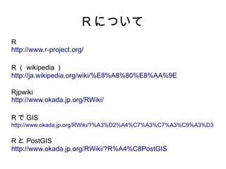
2. R について
R
http://www.r-project.org/
R （ wikipedia ）
http://ja.wikipedia.org/wiki/%E8%A8%80%E8%AA%9E
Rjpwiki
http://www.okada.jp.org/RWiki/
R で GIS
http://www.okada.jp.org/RWiki/?%A3%D2%A4%C7%A3%C7%A3%C9%A3%D3
R と PostGIS
http://www.okada.jp.org/RWiki/?R%A4%C8PostGIS

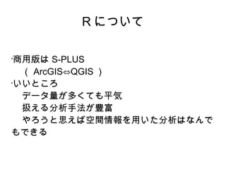
3. R について
•
商用版は S-PLUS
（ ArcGIS⇔QGIS ）
•
いいところ
データ量が多くても平気
扱える分析手法が豊富
やろうと思えば空間情報を用いた分析はなんで
もできる

4. R のインストール
windows, mac, linux で動作可能
•
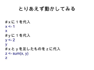
http://cran.md.tsukuba.ac.jp/

5. とりあえず動かしてみる
# x に 1 を代入
x <- 1
x
# y に 1 を代入
y <- 2
y
# x と y を足したものを z に代入
z <- sum(x, y)
z

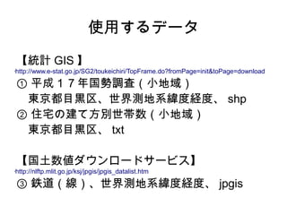
6. 使用するデータ
【統計 GIS 】
http://www.e-stat.go.jp/SG2/toukeichiri/TopFrame.do?fromPage=init&toPage=download
•
① 平成１７年国勢調査（小地域）
東京都目黒区、世界測地系緯度経度、 shp
② 住宅の建て方別世帯数（小地域）
東京都目黒区、 txt
【国土数値ダウンロードサービス】
http://nlftp.mlit.go.jp/ksj/jpgis/jpgis_datalist.htm
•
③ 鉄道（線）、世界測地系緯度経度、 jpgis

7. 概要

データのインポート

データの結合

データ加工

グラフの描画

クラスター分析

主題図の作成

8. おまじない
# パッケージのインストール
install.packages("maptools")
install.packages("cluster")
install.packages("RColorBrewer")
install.packages("classInt")
# パッケージの読み込み
library(maptools)
library(cluster)
library(RColorBrewer)
library(classInt)
# 作業ディレクトリの設定
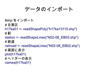
setwd(" フルパス ")

9. データのインポート
#shp をインポート
# 目黒区
h17ka01 <- readShapePoly("h17ka13110.shp")
#駅
station <- readShapeLines("N02-08_EB03.shp")
# 鉄道
railroad <- readShapeLines("N02-08_EB02.shp")
# 画面に表示
plot(h17ka01)
# ヘッダーの表示
names(h17ka01)

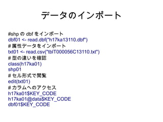
10. データのインポート
#shp の dbf をインポート
dbf01 <- read.dbf("h17ka13110.dbf")
# 属性データをインポート
txt01 <- read.csv("tblT000056C13110.txt")
# 型の違いを確認
class(h17ka01)
shp01
# セル形式で閲覧
edit(txt01)
# カラムへのアクセス
h17ka01$KEY_CODE
h17ka01@data$KEY_CODE
dbf01$KEY_CODE

11. データの結合
①merge
②spcbind
③dbf 差し替え
#merge すると型が変わる
tmp <- merge(h17ka01, txt01, by="KEY_CODE")
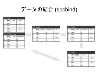
class(tmp)

12. データの結合 (spcbind)
① txt01
KEY_CODE ・・・・
1 0010 ・・・・
2 1001 ・・・・
③ txt02 ④ txt03
3 1002 ・・・・
KEY_CODE rowname ・・・・ KEY_CODE rowname ・・・・
4 1003 ・・・・
1 1001 3 ・・・・ 4 1004 0 ・・・・
② h17ka01.key
2 1002 2 ・・・・ 3 1003 1 ・・・・
KEY_CODE rowname
3 1003 1 ・・・・ 2 1002 2 ・・・・
0 1004 0
4 1004 0 ・・・・ 1 1001 3 ・・・・
1 1003 1
2 1002 2
3 1001 3
⑤ txt03
KEY_CODE rowname ・・・・
0 1004 0 ・・・・
1 1003 1 ・・・・
2 1002 2 ・・・・
3 1001 3 ・・・・

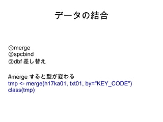
13. データの結合 (spcbind)
#spcbind
#②
h17ka01.key <- subset(h17ka01@data,,c(KEY_CODE))
h17ka01.key$rowname <- c(1:nrow(h17ka01.key)-1)
#③
txt02 <- merge(h17ka01.key, txt01, by="KEY_CODE")
#④
txt03 <- txt02[order(txt02$rowname),]
#⑤
rownames(txt03) <- c(1:nrow(txt03)-1)
# 結合
h17ka03 <- spCbind(h17ka01, txt03)

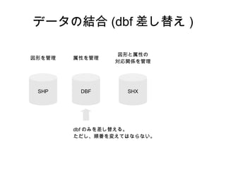
14. データの結合 (dbf 差し替え )
図形と属性の
図形を管理 属性を管理
対応関係を管理
SHP DBF SHX
dbf のみを差し替える。
ただし、順番を変えてはならない。

15. データの結合 (dbf 差し替え )
#dbf 差し替え
# 番号をふる
dbf01$no <- c(1:nrow(dbf01))
# 結合
merge01 <- merge(dbf01, txt01, by = "KEY_CODE")
# 並び順を元に戻す
merge02 <- merge01[order(merge01$no),]
#dbf をエクスポートし差し替える
（欠損値を含むレコードがあるとエラーが出るが無視）
write.dbf(dataframe=merge02, file="h17ka13110.dbf")

16. ひとやすみ
# 関数の help
help(readShapePoly)
各パッケージのドキュメント
http://cran.r-project.org/web/packages/maptools/maptools.pdf
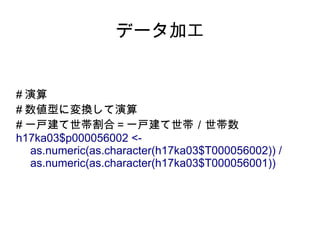
http://cran.r-project.org/web/packages/sp/sp.pdf

17. データ加工
# 演算
# 数値型に変換して演算
# 一戸建て世帯割合＝一戸建て世帯／世帯数
h17ka03$p000056002 <-
as.numeric(as.character(h17ka03$T000056002)) /
as.numeric(as.character(h17ka03$T000056001))

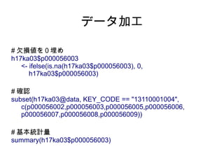
18. データ加工
# 欠損値を０埋め
h17ka03$p000056003
<- ifelse(is.na(h17ka03$p000056003), 0,
h17ka03$p000056003)
# 確認
subset(h17ka03@data, KEY_CODE == "13110001004",
c(p000056002,p000056003,p000056005,p000056006,
p000056007,p000056008,p000056009))
# 基本統計量
summary(h17ka03$p000056003)

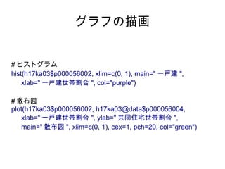
19. グラフの描画
# ヒストグラム
hist(h17ka03$p000056002, xlim=c(0, 1), main=" 一戸建 ",
xlab=" 一戸建世帯割合 ", col="purple")
# 散布図
plot(h17ka03$p000056002, h17ka03@data$p000056004,
xlab=" 一戸建世帯割合 ", ylab=" 共同住宅世帯割合 ",
main=" 散布図 ", xlim=c(0, 1), cex=1, pch=20, col="green")

20. クラスター分析
# クラスター分析に投入する項目を抽出
cluster01 <- h17ka03@data[,
c("p000056002","p000056003","p000056005",
"p000056006","p000056007","p000056008","p000056009")]
# クラスター分析の実行
cluster02 <- pam(cluster01, k=3)
# クラスター分析の結果
cluster.nm <- cluster02$clustering
# 図形データに結合
h17ka04 <-spCbind(h17ka03, cluster.nm)

21. クラスター分析の結果の解釈
# クラスターのグループごとに一戸建世帯割合を集計（平均）
barplot(by(h17ka04$p000056002,h17ka04$cluster.nm,mean),
main=" 一戸建 ")
#1 ；共同住宅３～５階建が多い
#2 ；一戸建が多い
#3 ；共同住宅６～階建が多い

22. 主題図の作成
#shp へエクスポート
writePolyShape(h17ka04, "cluster.shp")
# 閾値の数
class <- classIntervals(h17ka04$cluster.nm, 3)
# 色の設定
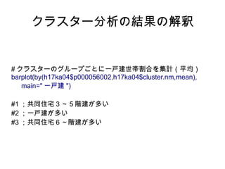
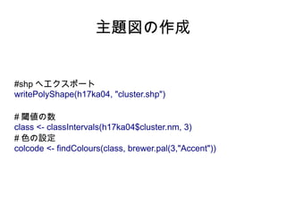
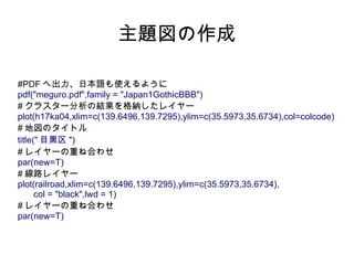
colcode <- findColours(class, brewer.pal(3,"Accent"))

23. 主題図の作成
#PDF へ出力、日本語も使えるように
pdf("meguro.pdf",family = "Japan1GothicBBB")
# クラスター分析の結果を格納したレイヤー
plot(h17ka04,xlim=c(139.6496,139.7295),ylim=c(35.5973,35.6734),col=colcode)
# 地図のタイトル
title(" 目黒区 ")
# レイヤーの重ね合わせ
par(new=T)
# 線路レイヤー
plot(railroad,xlim=c(139.6496,139.7295),ylim=c(35.5973,35.6734),
col = "black",lwd = 1)
# レイヤーの重ね合わせ
par(new=T)

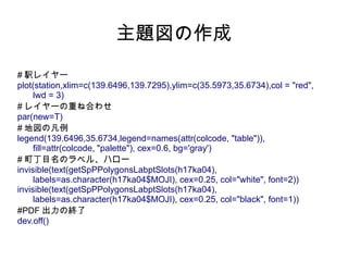
24. 主題図の作成
# 駅レイヤー
plot(station,xlim=c(139.6496,139.7295),ylim=c(35.5973,35.6734),col = "red",
lwd = 3)
# レイヤーの重ね合わせ
par(new=T)
# 地図の凡例
legend(139.6496,35.6734,legend=names(attr(colcode, "table")),
fill=attr(colcode, "palette"), cex=0.6, bg='gray')
# 町丁目名のラベル、ハロー
invisible(text(getSpPPolygonsLabptSlots(h17ka04),
labels=as.character(h17ka04$MOJI), cex=0.25, col="white", font=2))
invisible(text(getSpPPolygonsLabptSlots(h17ka04),
labels=as.character(h17ka04$MOJI), cex=0.25, col="black", font=1))
#PDF 出力の終了
dev.off()